Louisiana State UniversityLSU Digital Commons

LSU Master's Theses Graduate School

2003

Application of mechanistic models in predictingflow behavior in deviated wells under UBDconditionsFaisal Abdullah ALAdwaniLouisiana State University and Agricultural and Mechanical College, faladw1@lsu.edu

Follow this and additional works at: https://digitalcommons.lsu.edu/gradschool_theses

Part of the Petroleum Engineering Commons

This Thesis is brought to you for free and open access by the Graduate School at LSU Digital Commons. It has been accepted for inclusion in LSUMaster's Theses by an authorized graduate school editor of LSU Digital Commons. For more information, please contact gradetd@lsu.edu.

Recommended CitationALAdwani, Faisal Abdullah, "Application of mechanistic models in predicting flow behavior in deviated wells under UBD conditions"(2003). LSU Master's Theses. 2399.https://digitalcommons.lsu.edu/gradschool_theses/2399

APPLICATION OF MECHANISTIC MODELS IN PREDICTING FLOW BEHAVIOR IN DEVIATED WELLS UNDER UBD CONDITIONS

A Thesis

Submitted to the Graduate Faculty of the Louisiana State University and

Agricultural and Mechanical College in partial fulfillment of the

Requirements for the degree of Master of Science in Petroleum Engineering

in The Department of Petroleum Engineering

by Faisal Abdullah ALAdwani

B.Sc., Kuwait University, 1998 May, 2003

ii

Acknowledgements

At this opportunity the author would like to express great appreciation to Dr. Jeremy K.

Edwards for supervising this work and his valuable guidance and genuine interest in completing

this study. The author is greatly indebted to his country, Kuwait, for supporting his education

through the scholarship from Kuwait University. Also special thanks extend to the other

members of the committee, Dr. Julius Langlinais and Dr. John Smith for their valuable advice

and suggestions. In addition, a special thanks extends to Mr. Adel AL-Khayat from KUFPEC on

his advice on field operations. Finally, the author is grateful to the LSU Craft & Hawkins

department of petroleum engineering for giving the opportunity to complete this study under

their supervision.

iii

Table of Contents ACKNOWLEDGEMENTS………………………………………………………………………ii

LIST OF TABLES………………………………………………………………………………..iv

LIST OF FIGURES……………………………………………………………………………….v

ABSTRACT………………….…………………………………………………………………..vi

CHAPTER 1 – INTRODUCTION………………...…………………………………….………..1

CHAPTER 2 – LITERATURE REVIEW....……...………………………………………………3

CHAPTER 3 - MODEL DEVELOPMENT………………………………………………………6 3.1 Model Assumptions……………………………...……………………………………6 3.2 Multiphase Flow Concepts……………………………………………………………7

3.2.1 Liquid Holdup…………………………………………………….…………7 3.2.2 Superficial Velocity……………………………………………..…………..8 3.2.3 Fluid Properties……………………………………………...………………9 3.2.4 Two Phase Flow Patterns……………………………………………………9 3.2.5 UBD Flow Patterns………………………………...……………………....12

3.3 Flow Pattern Prediction Models………………………….………………..…………13 3.3.1 Downward Flow through the Drillstring………………………...…………13 3.3.2 Upward Flow through the Annuli………………...………..…..…………..16

3.4 Flow Behavior Prediction Models………………………………………...…………18 3.4.1 Downward Flow through the Drillstring…..……………………………….19 3.4.2 Upward Flow through the Annulus…..………………….………………....23

3.5 Bit Model…………………………………………………………….………………26 3.6 Fluid Properties………………………………………………………...……………27

CHAPTER 4 - COMPUTER MODEL…………………………………………………………..28 4.1 Field Example………………………………………………………………………..29

CHAPTER 5 – CONCLUSIONS AND RECOMMENDATIONS………………….………….39 5.1 Conclusions……………………………………………………………….…………39 5.2 Recommendations………………………….………………………………………..40

REFERENCES. ……………………………………..….………...…………………..…………41

APPENDIX A: PVT Correlations............................................................…….........…....………45

APPENDIX B: NOMENCLATURE ...……………………………………………………….…47

VITA……………………………………………………………………………………………..49

iv

List of Tables

3.1 Flow Coefficients for Different Inclination Angles…..................................………14

4.1 Drillstring and Annular Geometries for the Two Simulation Runs…….…..………34

4.2 Computer Program Input…...............……………………………………....…….…34

4.3 Comparison of Absolute Average Error for the Two Simulation Runs……..…..….35

A.1 Constants Used in Drunchak and Abu-Kassem Correlation………………………...45

v

List of Figures 3.1 Different Flow Patterns in Two Phase Flow………………………..………………………..10

3.2 Flow Pattern Map for Downward Two Phase Flow in Pipes (After Taitel et al.)………………..…….……………………………………………………….….…………….11 3.3 Flow Patter Map for Upward Two Phase Flow in Annulus (After Caetano et al.)…………………….…………………………………………………………..……………...12 3.4 Near Surface Annular Flow Pattern in UBD Operations (After Perez-Tellez et al.)…….......13 4.1 Incremental Wellbore Calculations Path in a Deviated Wellbore………........………...……30

4.2 Flowchart for the Computer Algorithm Used in the Mechanistic Steady State Model……...31 4.3 Well Suspension Diagram……………………………………………………………………32

4.4 Survey Plot of True Vertical Depth vs. Horizontal Departure….……………………………33

4.5 Comparison between Field Measurements and Simulators Output at Both Runs…………...36

4.6 Composite Plot of Pressure Distribution along with Well Geometry for Run #1.…...……...37

4.7 Simulation Results (Hl, ∆P/∆L) vs. Depth at Run #2 in the Annulus…….……..………..….38

vi

Abstract

Underbalanced drilling (UBD) has increased in recent years because of the many

advantages associated with it. These include increase in the rate of penetration and reduction of

lost circulation and formation damage. Drilling of deviated and horizontal wells also increased

since recovery can be improved from a horizontal or a deviated well. The drilling of deviated

wells using UBD method will reduce several drilling related problems such as hole cleaning and

formation damage. Prediction of flow and pressure profiles while drilling underbalanced in such

wells will help in designing and planning of the well. The main aim of this research is to study

and model the effect of well deviation on pressure and flow profile in the drillstring and the

annulus under UBD conditions through the use of mechanistic two phase flow models.

Specifically, a current model is modified to include effects of wellbore deviation. Simulation

results are compared with data from a deviated well drilled with UBD technology.

1

Chapter 1

Introduction

Underbalanced drilling is the drilling process where the effective bottomhole circulation

pressure of the fluid system is less than the formation pressure. UBD can be achieved by

injecting lightened drilling fluid such as gas, mist, foam, and diesel, which will create such low

pressure in order not to overcome the formation pressure.

The main reasons to perform UBD operations are listed below1.

• Increased bit life and rate of penetration.

• Minimize lost circulation and differential sticking.

• Reduce formation damage and stimulation requirements.

• Environmental benefits.

Performing UBD operations on deviated or horizontal wells requires controlling the

drilling parameters in order not to damage the formation and to achieve the maximum rate of

penetration. In order to optimize the use of UBD in any well, a successful control of the

bottomhole pressure and fluid flowing through the formation is necessary.

Some of the damage mechanisms that may occur in both horizontal and vertical wells are

listed below2:

• Rock and fluid flow incompatibilities.

• Solid invasion.

• Chemical adsorption/wettability.

• Fines migration.

• Biological activities.

2

In addition, some of the damages that occurs during UBD operations may include:

• Lack of protective sealing filter cake.

• Spontaneous countercurrent imbibition effects, which allow the entrainment of

potentially damaging fluid filtrate into the reservoir matrix in the near wellbore

region.

• Glazing and surface damage effects caused by insufficient heat conductivity

capacity of circulating fluids.

During UBD operations, a complex fluid system occurs both inside the drillstring and the

annulus. Two phase flow prediction techniques are used to predict several parameters such as

pressure drops (both inside the drillstring and through the annulus), flow patterns, velocities,

liquid holdup, and other parameters. In order to achieve this task, a set of mechanistic two phase

flow models are used. It has been shown in the literature that mechanistic models accurately

predict the flow pattern and liquid holdup. These models are based on the physical phenomena of

the complex fluid system and flow rather than the use of empirical correlations, which are based

mainly on experimental data.

3

Chapter 2

Literature Review

Several techniques are used in order to achieve the optimum result while performing

UBD operations. The main approach used to predict the flow behavior of wells under UBD

conditions is the use of the two phase flow concepts. Currently available computer models use

different approaches for predicting the behavior under such conditions. Three main approaches

are used in the development of such computer models, as follows :

• Homogenous approach.

• Empirical correlations approach.

• Mechanistic approach.

The homogenous approach was first used by Guo et al3. Their model calculated the

required air rate for both maximum rate of penetration and cutting transport in foam drilling

operations. They assumed that the foam can be treated as a two phase fluid in the bubbly region

despite the fact that they recognized the main flow patterns (bubble, slug, churn, and annular).

The empirical correlations are formulated by establishing a mathematical relation based

on experiments. Application of empirical models is limited to the data range used to generate the

model. Liu et al4 developed a computer algorithm which analyzed the behavior of foam in UBD

operation, considering it as a two phase mixture. They calculated the frictional pressure drop

using the mechanical energy equation coupled with a foam rheology model using an equation of

state. In addition, they united their model with the Beggs and Brill5 method for calculating

bottomhole pressure and developed a computer program called MUDLITE6,7. The current

version of MUDLITE includes other two phase flow correlations in addition to Beggs and Brill

such as Orkiszewski, Hagedorn-Brown, and others. Despite the fact that the used correlation

4

gives good results under certain flow conditions (such as stable flow in an oil well) none of the

previous models were developed for actual field conditions. Tian8,9 developed a commercial

computer program named Hydraulic UnderBalanced Simulator (HUBS), which was used in

assisting engineers to design UBD operations especially for the process of optimizing circulation

rate and obtaining sufficient hole cleaning. HUBS uses empirical correlations for the UBD

hydraulic calculations in addition to the developed mathematical model.

Mechanistic models were developed significantly in recent years. Those models are based

on a phenomenological approach that takes into account basic principles (conservation of mass

and energy). Bijleveld et al.10 developed the first steady state computer program using

mechanistic approach where bottomhole pressure and two phase flow parameters were calculated

by using a trial and error procedure. Stratified flow was initially assumed and then checked for

validity. If the guessed flow pattern does not exist, another flow pattern is assumed and the same

procedure is repeated. An average absolute error of 10% was reported compared with an average

absolute error of 12% shown by Beggs and Brill. Several authors developed mechanistic models

to predict accurately different flow parameters such as flow pattern, film thickness, rise velocity

of gas bubbles in liquid columns, and liquid holdup. Ansari et al.11 presented his model for

upward vertical two phase flow in pipes. They did not include any effect of inclination although

it exists in the model. Gomez, et al.12 develped a unified mechanistic model for predicting the

flow parameters while Kaya et al.13 developed a comprehensive mechanistic model for

predicting the flow parameters in deviated wells. Caetano et al.14,15 developed a model for

upward vertical flow in the annulus. Hasan and Kabir16 developed a model for predicting two

phase flow in annuli where they estimated the gas void fraction in during upward simultaneous

two phase flow by using the drift flux approach between the liquid slug and the Taylor bubble.

Lage et al.17 developed a mechanistic model for predicting upward two phase flow in concentric

5

annulus. Recently, Perez-Tellez et al.18 developed an improved, comprehensive mechanistic

steady state model for pressure prediction through a wellbore during UBD operations in vertical

wells; the model was validated against an actual well and full-scale well data, where it shows

good performance (absolute average error less than 5%).

Gavignet and Sobey19 reported that the drill pipe eccentricity has a large effect on the bed

thickness. They reported that once the interfacial area decreases with increasing in the thickness

of the cutting bed in deviated well. Hence in order to maintain an adequate movement of the mud

in the annulus a large increase in the velocity is required to maintain interfacial friction carrying

the cuttings up the annulus. In a deviated well, the pipe is most likely to be in an eccentric

geometry in certain location. In addition Brown and Bern20 stated that the extremes positions that

reflect a realistic downhole position of drillpipe is an eccentricity of 75% which most likely

occurs by a tool joint touching the bottom of the hole in a drillpipe centralized in the casing at

limiting position.

6

Chapter 3

Model Development

The key factor for a successful UBD operation is to achieve the objectives for switching

to UBD as discussed in Chapter 1. In order to achieve such success, the bottomhole pressure

should be maintained within a pressure window that is bounded by below by the formation pore

pressure and above by the wellbore stability pressure or surface facilities restrictions. Hence, the

prediction of wellbore pressure should be as accurate as possible in order to assist in designing

equipment needed to switch to UBD operations. In the past, the key approach used to predict

wellbore pressure has been to use empirical multiphase flow correlations. As discussed in

Chapter 2, those techniques often do not accurately match the field cases in which we are

interested. In addition, those correlations are typically valid only for the range of conditions used

to create the correlation.

Recently, development of mechanistic models has allowed accurate prediction of

wellbore pressure. Many UBD operations require the use of nitrified diesel as the drilling fluid.

Thus two phase flow will exist both in the drill pipe and the annulus. In addition, the procedure

used to apply those mechanistic models in order to accurately predict wellbore pressure will be

discussed, along with the major assumptions used in the model development.

3.1 Model Assumptions

In most UBD operation the drilling fluid (gasified liquid) is injected in the drillstring

down through the bit and then up the annulus, where it will mix with formation rock cuttings and

produced fluids form the formation.

The following assumptions were needed in order to model the behavior of a UBD

operation as a two phase flow system in which only gas and liquid exists.

7

• The injection and formation fluids (liquid and gas) will flow at the same velocity.

• Mixture velocity and viscosity will be used instead of the usual mud cleaning

rheology models because of the turbulent hole cleaning produced by the high

friction gradients which results from multiphase flow of the mixture of injected

and produced fluids.

• Effects of cutting transport are neglected.

3.2 Multiphase Flow Concepts

During the simultaneous flow of gas and liquid, the most distinguished aspect of such

flow is the inconsistency of the distribution of both phases in the wellbore. The term flow pattern

is used to distinguish such distribution, which depends on the relative magnitude of forces acting

on the fluids21. The following terms are defined in order to assist in the multiphase flow

calculations.

3.2.1 Liquid Holdup

Liquid holdup (HL) is defined as the fraction of a pipe cross-section or volume increment

that is occupied by the liquid phase22. The value of HL ranges from 0 (total gas) to 1 (total

liquid). The liquid holdup is defined by

P

LL A

AH = 3.1

where AL is the pipe area of the liquid occupied by the liquid phase and AP is pipe cross-

sectional area.

The term void fraction or gas holdup is defined as the volume fraction occupied by the gas where

LH−= 1α 3.2

8

When the two fluids travel at different velocities then the flow is referred to as a slip flow. No

slip flow occurs when the two fluids travels at the same velocity. Hence, the term no slip liquid

holdup can be defined as the ratio of the volume of liquid in a pipe element that would exist if

the gas and liquid traveled at the same velocity divided by the volume of the pipe element22. The

no-slip holdup (λL) is defined as follows:

GL

LL qq

q+

=λ 3.3

where qL is the in-situ liquid flow rate and qG is the in-situ gas flow rate.

3.2.2 Superficial Velocity

Superficial velocity is the velocity that a phase would travel at if it flowed through the

total cross sectional area available for flow22. Thus, the liquid and gas superficial velocities are

defined by :

P

LSL A

qv = 3.4

and

P

GSG A

qv = 3.5

The mixture velocity can be defined as the velocity of the two phases together, as follow :

SGSLP

GLM vv

Aqqv +=

+= 3.6

The in-situ velocity is the actual velocity of the phase when the two phases travel

together. They can be defined as follows :

9

L

SLL H

vv = 3.7

and

L

SG

G

SGG H

vHvv

−==

1 3.8

When water exists in addition to the liquid and gas, a weighting factor is introduced to take care

of the slippage that could occur between different liquid phases that exists during drilling

(drilling fluid, produced oil and produced water). This factor is defined as follows:

wODF

DFo qqq

qf++

= 3.9

where DFq is the drilling fluid flow rate, Oq inflow oil flow rate, and wq is inflow water flow

rate.

3.2.3 Fluid properties

Mixture fluid properties (density and viscosity) can be calculated for the case of no-slip

or slip flow. Mixture density and viscosity are calculated using a weighted average technique

based on the in-situ liquid holdup.

3.2.4 Two Phase Flow Patterns

As mentioned above, the variation in the physical distribution of the phases in the flow

medium creates several flow patterns. Multiphase flow patterns highly depend on flow rates,

wellbore geometry, and the fluid properties of the phases. In addition, flow patterns can change

with variation in wellbore pressure and temperature. The major flow patterns that exist in

multiphase flow are dispersed bubble, bubble, slug, churn and annular. Figure 3.1 shows

different flow patterns exists in a pipe.

10

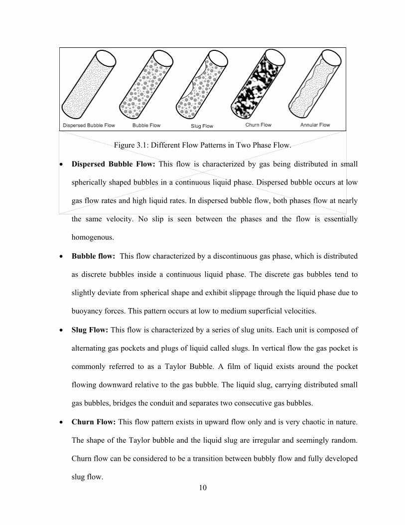
Figure 3.1: Different Flow Patterns in Two Phase Flow.

• Dispersed Bubble Flow: This flow is characterized by gas being distributed in small

spherically shaped bubbles in a continuous liquid phase. Dispersed bubble occurs at low

gas flow rates and high liquid rates. In dispersed bubble flow, both phases flow at nearly

the same velocity. No slip is seen between the phases and the flow is essentially

homogenous.

• Bubble flow: This flow characterized by a discontinuous gas phase, which is distributed

as discrete bubbles inside a continuous liquid phase. The discrete gas bubbles tend to

slightly deviate from spherical shape and exhibit slippage through the liquid phase due to

buoyancy forces. This pattern occurs at low to medium superficial velocities.

• Slug Flow: This flow is characterized by a series of slug units. Each unit is composed of

alternating gas pockets and plugs of liquid called slugs. In vertical flow the gas pocket is

commonly referred to as a Taylor Bubble. A film of liquid exists around the pocket

flowing downward relative to the gas bubble. The liquid slug, carrying distributed small

gas bubbles, bridges the conduit and separates two consecutive gas bubbles.

• Churn Flow: This flow pattern exists in upward flow only and is very chaotic in nature.

The shape of the Taylor bubble and the liquid slug are irregular and seemingly random.

Churn flow can be considered to be a transition between bubbly flow and fully developed

slug flow.

11

• Annular Flow: This flow pattern is characterized by the axial continuity of gas phase in

a central core with the liquid flowing upward, both as a thin film along the pipe wall and

as a dispersed droplets in the core. A small amount of liquid is entrained in the light

velocity core region. Annular flow occurs at high gas superficial velocities with relatively

little liquid present.

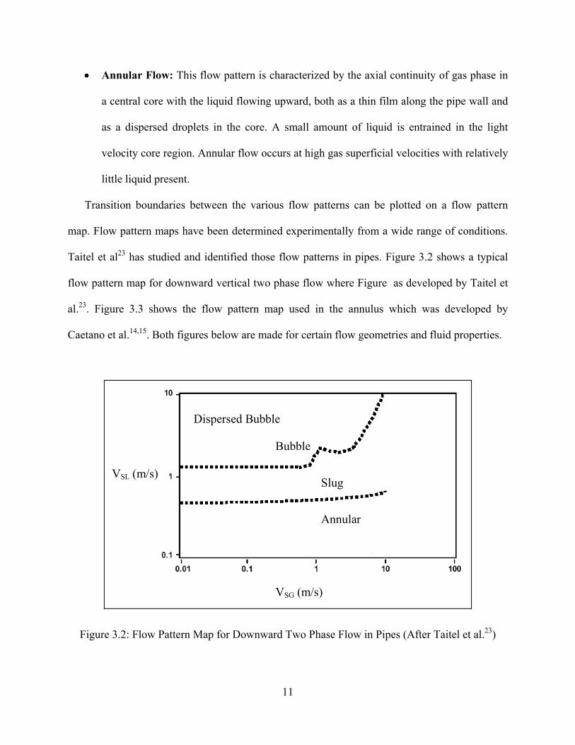
Transition boundaries between the various flow patterns can be plotted on a flow pattern

map. Flow pattern maps have been determined experimentally from a wide range of conditions.

Taitel et al23 has studied and identified those flow patterns in pipes. Figure 3.2 shows a typical

flow pattern map for downward vertical two phase flow where Figure as developed by Taitel et

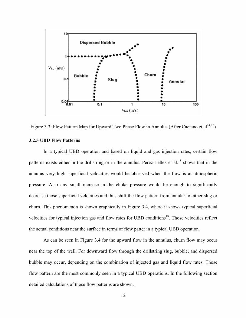
al.23. Figure 3.3 shows the flow pattern map used in the annulus which was developed by

Caetano et al.14,15. Both figures below are made for certain flow geometries and fluid properties.

Dispersed Bubble

Bubble

Slug

Annular

VSG (m/s)

VSL (m/s)

Figure 3.2: Flow Pattern Map for Downward Two Phase Flow in Pipes (After Taitel et al.23)

12

VSG (m/s)

VSL (m/s)

Figure 3.3: Flow Pattern Map for Upward Two Phase Flow in Annulus (After Caetano et al14,15)

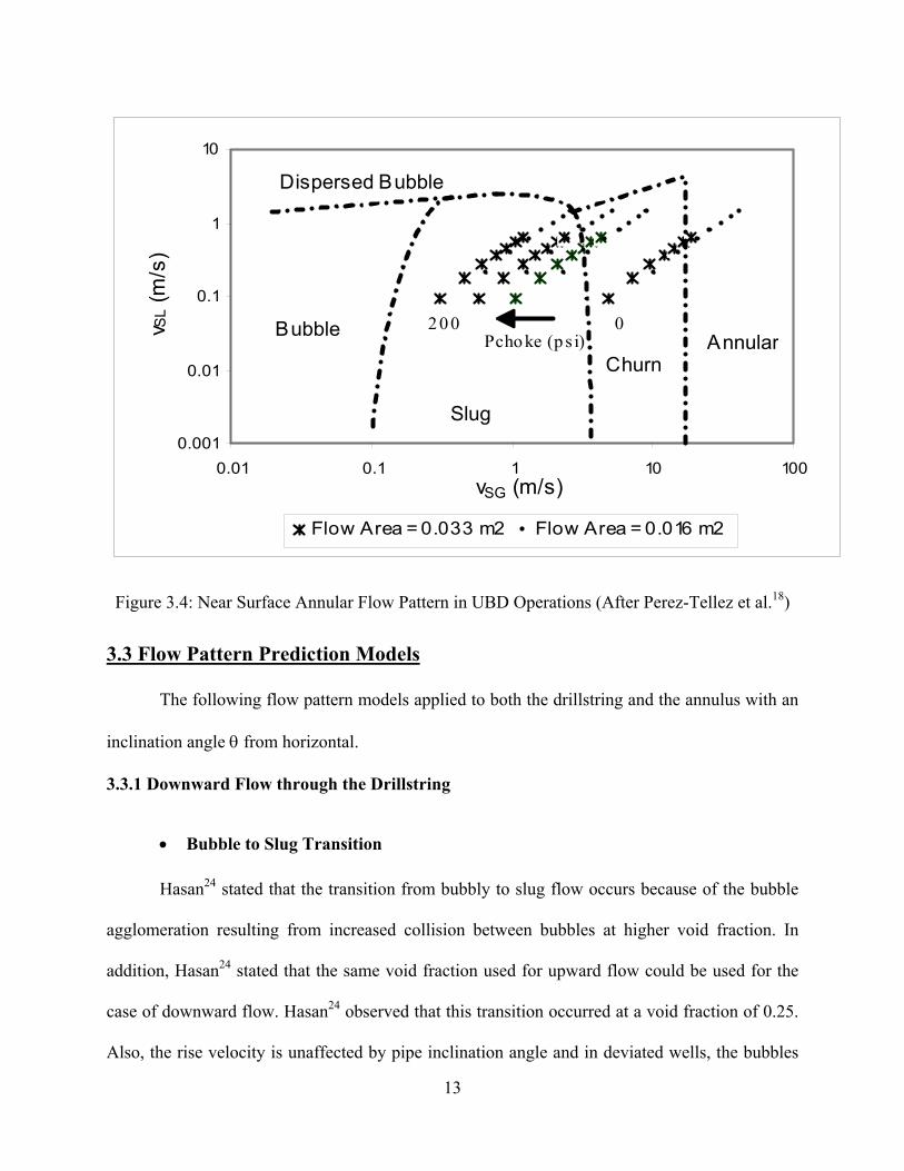
3.2.5 UBD Flow Patterns

In a typical UBD operation and based on liquid and gas injection rates, certain flow

patterns exists either in the drillstring or in the annulus. Perez-Tellez et al.18 shows that in the

annulus very high superficial velocities would be observed when the flow is at atmospheric

pressure. Also any small increase in the choke pressure would be enough to significantly

decrease those superficial velocities and thus shift the flow pattern from annular to either slug or

churn. This phenomenon is shown graphically in Figure 3.4, where it shows typical superficial

velocities for typical injection gas and flow rates for UBD conditions18. Those velocities reflect

the actual conditions near the surface in terms of flow patter in a typical UBD operation.

As can be seen in Figure 3.4 for the upward flow in the annulus, churn flow may occur

near the top of the well. For downward flow through the drillstring slug, bubble, and dispersed

bubble may occur, depending on the combination of injected gas and liquid flow rates. Those

flow pattern are the most commonly seen in a typical UBD operations. In the following section

detailed calculations of those flow patterns are shown.

13

0.001

0.01

0.1

1

10

0.01 0.1 1 10 100

S upe r f i c i a l Ga s Ve l oc i t y ( m/ s)

Flow Area = 0.033 m2 Flow Area = 0.016 m2

Pcho ke (p s i)02 0 0 Bubble

Churn

Slug

Dispersed Bubble

Annular

vSG (m/s)

vSL

(m/s

)

Figure 3.4: Near Surface Annular Flow Pattern in UBD Operations (After Perez-Tellez et al.18)

3.3 Flow Pattern Prediction Models

The following flow pattern models applied to both the drillstring and the annulus with an

inclination angle θ from horizontal.

3.3.1 Downward Flow through the Drillstring

• Bubble to Slug Transition

Hasan24 stated that the transition from bubbly to slug flow occurs because of the bubble

agglomeration resulting from increased collision between bubbles at higher void fraction. In

addition, Hasan24 stated that the same void fraction used for upward flow could be used for the

case of downward flow. Hasan24 observed that this transition occurred at a void fraction of 0.25.

Also, the rise velocity is unaffected by pipe inclination angle and in deviated wells, the bubbles

14

prefer to flow near the upper wall of the pipe, causing a higher local void fraction compared with

the cross-sectional average value24. Hasan25 and Hasan and Kabir26 derived an equation for

bubble to slug transition flow for upward flow in deviated wells. Hasan24 proposes the same

equation for a downward flow using a negative terminal rise velocity. Hasan24 proposed the

following expression for transition boundary between bubble and slug flow:

θα

sin)/1( O

SLOSG C

vvCv−−

= ∞ 3.10

Harmathy27 correlation is used to calculate the terminal rise velocity (ν∞) for upward flow in

vertical and inclined channels as follows:

( ) 25.0

253.1

−=∞

L

GL gvρ

σρρ 3.11

The velocity profile coefficient (CO) has been defined by Zuber and Findlay28 due to the effect of

non-uniform flow and concentration distribution across the pipe and the effect of local relative

velocity between the two phases. Table 3.1 shows the values for the velocity profile coefficients

for different inclination angles as given by Alves29

Table 3.1: Flow Coefficients for Different Inclination Angle Ranges (After Alves29)

Inclination Angle (Degrees) Co

10-50 1.05

50-60 1.15

60-90 1.25

In addition, Wallis30 has proposed that the effect of single bubble rising in a swarm of bubbles

can be introduced by defining a bubble swarm effect (n), thus nLH will be taken into

15

consideration. Finally, Perez-Tellez et al18 proposed the use of the combined effect of the bubble

swarm effect (n) and the velocity profile coefficient (CO) and introduced the following

expression for the bubble slug transition

nLmoG HvvCv ∞=− 3.12

Applying Equation 3.12 to Hasan approach in order to find the criteria from bubble to slug yields

the following equation

O

nLSGO

SL CHvvC

v ∞+−=

)sin(/)/1( θα 3.13

with a gas void fraction α = 0.25.

• Bubble or Slug to Dispersed Bubble Transition

Hasan and Kabir16 find that the model which was created by Taitel et al23 was applicable

for flow through vertical and inclined annuli. Based on the maximum bubble diameter possible

under highly turbulent conditions the model following model could be used to find the relation

ship between phase velocities, pipe diameters, and fluid properties24. Perez-Tellez31

recommended the use of the equation developed by Caetano14,15 as shown below where ID is the

inner pipe diameter.

( )

5.06.05.04.04.02.1 15.4725.06.12

+=

−

M

SGL

GL

FM v

vgID

fvσρ

ρρσ 3.14

Equation 3.14 shows that in order to calculate the homogenous fanning friction factor, and since

the rise velocity for the dispersed bubble flow is very small compared to the local velocities, the

no-slip holdup (λL) could be used to calculate fF.

16

3.3.2 Upward Flow through the Annuli

Several authors14,15,16,17 agreed on using the method proposed by Taitel et al23 for

predicting flow pattern, in addition to his model and coupling it with the bubble swarm effect

and the velocity swarm coefficient. The flow patterns used were shown in Figure 3.3 where the

transition boundaries will be calculated based on different flow geometry and properties.

• Bubble to Slug Transition

During bubble flow, discrete bubbles rise with the occasional appearance of a Taylor

bubble. The discrete bubble rise velocity was defined in Equation 3.11. Hasan and Kabir16 stated

that the presence of an inner tube tends to make the nose of the Taylor bubble sharper, causing

an increase in the Taylor bubble rise velocity. As a result, Hasan and Kabir15 developed Equation

3.15 where the diameter of the outer tube should be used with the diameter ratio (OD/ID) to get

the following expression for the Taylor bubble rise velocity in inclined annulus

L

GLTB gIDIDODv

ρρρθθ −

++= 2.1)cos1(sin))/(*1.0345.0( 3.15

where

OD : Outside pipe diameter

ID : Inner casing diameter

g : Gravity acceleration

ρL: Liquid density

ρG: Gas density

Hasan and Kabir16 stated that the presence of an inner tube does not appear to influence the

bubble concentration profile (CO) and thus the following expression could be used :

17

∞−−

= vvC

v SGOSL θsin

)4( 3.16

• Bubble or Slug to dispersed bubble transition

Equation 3.14 is used to define the transition from bubble or slug to dispersed bubble

flow. The hydraulic diameter (Dh) is substituted for the pipe inside diameter (ID). The hydraulic

diameter of the casing-tubing annulus is given by

Dh = ID – OD 3.17

where ID is the internal casing diameter and OD is the outside pipe diameter.

• Dispersed bubble to slug flow transition

Taitel et al.23 determined that the maximum allowable gas void fraction under bubble

flow condition is 0.52. Higher values will convert the flow to slug, hence the transition boundary

could be equated as follows :

SGSL vv 923.0= 3.18

• Slug to churn transition

Tengesdal et al.32 has developed a transition from slug to churn flow in an annulus. They

stated that the slug structure will be completely destroyed and churn flow will occur if the gas

void fraction equals 0.78. Thus churn flow will occur. The transition from slug flow to churn

flow can thus be represented by :

epsgSL gDvv 292.00684.0 −= 3.19

where Dep is the equi-periphery diameter defined as follow

Dep = ID + OD 3.20

18

where ID is the inner casing diameter and OD is the outer pipe diameter.

• Churn to annular transition

Taitel et al.23 proposed the following transition which was supported by Hasan and

Kabir16 :

( ) 25.0

21.3

−=

G

GLSG

gvρ

σρρ 3.21

3.4 Flow Behavior Prediction Models

After determining the required flow pattern, which either exists in the drillstring or

annulus, then the following behavior prediction models are applied in order to calculate the

pressure gradient and phases fractions. The total pressure gradient is calculated as follows :

accfeltotal dLdP

dLdP

dLdP

dLdP

+

+

=

3.22

Where the following are the component of the total pressure gradient

eldLdP

is the elevation change component

fdLdP

is the friction component

accdLdP

is the acceleration component

19

3.4.1 Downward Flow through the Drillstring

• Bubble Flow Model for Drillstring

The drift flux approach is used to calculate liquid holdup considering the slippage

between the phases and non-homogenous distribution of bubbles. Kaya et al.13 developed an

expression for the slip velocity considering inclination and bubble swarm effect. Assuming

turbulent velocity profile for the mixture with rising bubbles concentrated more at the center than

along the pipe wall, the slip velocity using the drift flux approach can be expressed as follows:

MOL

SGS vC

Hvv −−

=1

3.23

With an inclination angle θ the proposed model13 as shown below

θsinLS Hvv ∞= 3.24

Combining equations 3.23 and 3.24 we get the following expression

ML

SGL v

HvHv 2.1

1sin −

−=∞ θ 3.25

Liquid holdup can be calculated from Equation 3.25 using a trial and error procedure as follow

1. Assume an initial holdup value (HL0); a good guess is the no-slip holdup.

2. Calculate the holdup Equation 3.25 as follows :

ML

SGL vHv

vH2.1sin

1+

−=∞ θ

3.26

3. Check the calculated value with the guessed one. If the two values of HL agree within an

acceptable tolerance then stop. Otherwise, repeat steps 1-3 until HL converges.

After determining the holdup, mixture properties can be calculated using the following equations

20

)1( LGLLM HH −+= ρρρ 3.27

)1( LGLLM HH −+= µµµ 3.28

The elevation pressure gradient is given by

θρ singdLdP

Mel

=

3.29

The frictional pressure loss is given by

IDvf

dLdP MMM

f 2

2ρ=

3.30

where ID is the inner pipe diameter and fM is the Moody friction factor and is calculated using the

following Reynolds number

M

MMMRE

IDvNµ

ρ=, 3.31

Moody friction factor is four times the Fanning friction factor and it is calculated using the

Colebrook33 function and solving using a trial and error procedure using the Equation 3.32 :

+−=

mREm fNIDf255.1269.0log41 ε 3.32

where

ID: inner pipe diameter

NRE: Reynolds number and

ε: pipe roughness.

The acceleration pressure gradient components is calculated using Beggs and Brill5 approach as

follow

21

dLdP

pvv

dLdP SGMM

acc

ρ=

3.33

the acceleration term (Ek) is defined as follow

pvvE SGMM

kρ

= 3.34

Then the total pressure drop is calculated by Equation 3.35 :

k

fel

total EdLdP

dLdP

dLdP

−

−

=

1 3.35

• Dispersed bubble flow model for drillstring

Since nearly a uniform bubble distribution in the liquid, the flow can be treated as a

homogenous flow. Thus, the liquid holdup is very close to the no-slip holdup (λL). Hence, the

total pressure drop is calculated using Equations 3.27-3.35.

• Slug flow model for drillstring

From the bubbly flow model shown above, liquid holdup for the rise velocity of a Taylor

bubble in downward flow may be calculated by

( )TBm

SGL vvC

vHTB −

−=1

1 3.36

Hasan24 recommended to use a value of C1=1.12. The liquid holdup is calculated by Equation

3.37 :

( ) ( )

−+−−=

LSTBSU LSU

LSL

SU

TBL H

LL

HLL

H 111 3.37

22

The slug unit length can be calculated by the following expression based on the superficial gas

velocity

sec4.0for )(160

0

mvvvCvIDL SG

m

SGSU >

−=

∞

3.38

sec4.0for 64

0

mvvvC

IDL SGm

SU ≤−

=∞

3.39

Perez-Tellez31 showed that, for a fully developed Taylor bubble, the total hydrostatic and

frictional pressure losses can be calculated by

( )[ ]gdLdP

TBLS MMel

βρρβ +−=

1 3.40

( )βρ

−=

1

2 2

IDvf

dLdP MMF

f

LSLS 3.41

The acceleration component in the drillstring can be calculated by using Equations 3.33-3.35.

For fully developed Taylor bubble flow condition, β is given by

SUTB LL /=β 3.42

and GMTBρρ =

where LSMρ is calculated as in Equation 3.27 with changing HL with

LSLH , in addition the friction

factor is calculated using the following mixture Reynolds number

)1(,LSLS

LS

LGLL

MMMRE HH

IDvN

−+=

µµρ

3.43

23

3.4.2 Upward Flow through the Annulus

• Bubble Flow Model for Annular Geometries

For a bubbly flow the holdup is calculated as reported by Hasan and Kabir15 as follows :

MO

SGL vCv

vH

−−=

∞

1 3.44

CO values are based on the inclination angle as shown in Table 3.1.

After calculating the holdup then mixture density and viscosity are calculated from Equations

3.27 and 3.28. The elevation pressure gradient is calculated using equation 3.29. For the

frictional pressure loss is calculated from equation 2.30. Caetano14,15 suggested the use of the

calculation developed by Gunn and Darling34 for a turbulent flow as follow

[ ] [ ]4.0log4

5.010/)3000(exp45.0

Re

5.010/)3000(exp45.0 66

−

=

−−

−−− RERE N

CA

PF

N

CA

PF F

FfNFFf 3.45

where fF is the Fanning friction factor.

Equation 3.45 has the following parameters:

FP and FCA are geometry parameters defined by the following equations

FP=16/NRE 3.46

−−

−−

−=

)/1ln(1

11

)1(162

2

4

2

KK

KK

KFCA 3.47

K: diameter ratio is defined below

K=OD/ID 3.48

Where OD is the pipe outer diameter and ID is the inner casing diameter.

24

The mixture Reynolds number is calculated using Equation 3.31 the hydraulic diameter (Dh)

used instead of the pipe inside diameter (ID).

The acceleration component is calculated using Beggs and Brill5 approach using Equations 3.33-

3.35

• Dispersed Bubble Flow Model

The dispersed bubble holdup is assumed equal to the no-slip holdup (λL). The same

equations as in the bubble flow are used to calculate the total pressure gradient.

• Slug Flow Model

The same model used by Perez-Tellez31 for the case of downward flow inside the

drillstring is used. The hydraulic diameter is used instead of the inner tubing diameter in

Equation 3.43 for calculating Reynolds number. In addition, the acceleration component can be

calculated by

( )( )LSTBLS

LSLTBLL

SU

LL

acc

vvvvL

HdLdP

−+=

ρ

3.49

Finally the average holdup over the entire slug unit SULH for either developed of fully developing

Taylor bubble can be calculated by18

( )( )TB

GTBLSGL v

vvHvH LSLS

SU

−−+−=

11 3.50

• Annular flow model

Perez-Tellez31 suggested using the model developed by Taitel and Barnea35, where he

stated that the use of this model will avoid convergence problems when implementing it into the

computations.

25

Taitel and Barnea35 stated that the total pressure drop in an annular flow can be calculated

as follows :

θρρδ

τ SingHHD

rdLdP

LGLLe

i

total

)]1([2

−++−

=

3.51

The annular film thickness can be defined as follow

6.03/12

)(115.0

−

=L

eSLL

LGL

L Dvg µ

ρρρρ

µδ 3.52

De is the equivalent pipe diameter and is calculated by

22 ODIDDe −= 3.53

where ID is the inner casing diameter and OD is the outer pipe diameter.

The interfacial shear stress (τi) is defined by

[ ]4

2

)/(215.0

e

SGGii D

vfδρ

τ−

= 3.54

The interfacial shear friction factor is calculated as suggested by Alves et al35 as follows :

fi=fscI 3.55

where fcs is the superficial core friction factor (gas phase) and is calculated based on the core

superficial velocity, density and viscosity. The interfacial correction parameter I is used to take

into account the roughness of the interface. The parameter I is an average between the horizontal

angle and the vertical angle and is calculated based on an inclination θ

Iθ=IH cos2θ + IV sin2 θ 3.56

The horizontal correction parameter is given by Henstock and Hanratty36 :

26

IH=1+800FA 3.57

where

[ ] 5.0

9.0,

4.05.29.0,

5.22, )0379.0()707.0(

+=

G

L

G

L

SGRE

SLRESLREA v

vN

NNF

ρρ 3.58

Where NRE,SL and NRE,SG are the superficial liquid and gas Reynolds number respectively. Both

are calculated below

L

SLLSLRE

IDvNµ

ρ=, 3.59

and

G

SGLSGRE

IDvNµ

ρ=, 3.60

The vertical correction parameter is given by Wallis37 as follow

IV=1+300(δ/De) 3.61

Finally considering a constant liquid film thickness, the liquid holdup can be calculated by

−=

2

4ee

L DDH δδ 3.62

3.5 Bit Model

Perez-Tellez31 developed a two phase bit model to handle the pressure drop across the bit

nozzles. Using the mechanical energy balance38 along with the gas weighting fraction and

neglecting frictional pressure drop, he formulated the following expression for calculating the

pressure drop across the bit nozzles :

27

0ln)()1(2

=

+−

−+

up

bh

g

gupbh

L

g

c

n

PP

MzRTw

PPw

gv

ρ 3.63

where

vn is the nozzle velocity

wg is the gas weighing factor

Pbh is the bottomhole pressure

Pup is the upstream pressure

Mg is the gas molecular weight

Also using the continuity equation for the gas liquid mixture the following expression is reached

to express the conservation of mass

constant=+= GGLLnMM qqAv ρρρ 3.64

And the nozzle velocity is calculated by

vA

qqvn

LLGGn

ρρ += 3.65

The above three equations are solved numerically to obtain the bit nozzle upstream pressure

given the bottomhole pressure.

3.6 Fluid Properties

Several fluid properties need to be calculated when carrying the analysis either in the

drillstring or the annulus. Several authors have published correlations for calculating such

properties. Appendix A shows the calculations used to compute such properties.

28

Chapter 4

Computer Model

In Chapter 3, it was discussed how to utilize the mechanistic steady state model in order

to model the flow behavior of an inclined well during UBD operation. In this work, the computer

algorithm that was developed by Perez-Tellez31 was modified and adjusted to handle a deviated

wellbore. Specifically it was used to find a solution for the bottomhole pressure using the

mechanistic models discussed previously.

The algorithm was coded into a macro which can be run using MS EXCEL®. The macro

was written in VBA® (Visual Basic for Applications). Creating the code in EXCEL makes it easy

to continue the analysis further into the same application or link it with other applications.

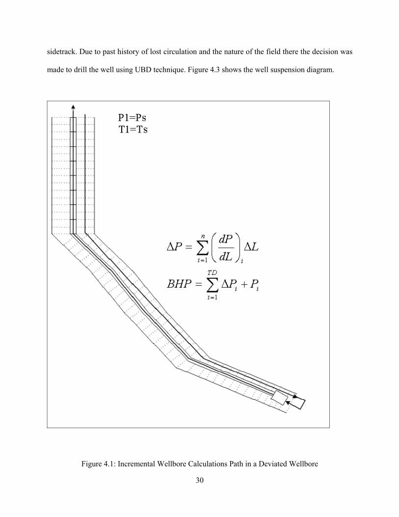
An incremental procedure for calculating the wellbore pressure traverse is used by the

program. Increments of depth ∆Li with an inclination angle θi from the horizontal. Figure 4.1

shows typical incremental calculations diagram in a deviated wellbore when carrying such type

of pressure traverse calculations. As shows Figure 4.1, the calculations start at the annulus with a

known starting pressure point (choke, surface) and then the calculations continue through the

annulus taking into account different wellbore inclinations and different casing and drill pipe

geometries. Inclination angles are read from the survey file and then a simple linear interpolation

is used to find the angle at any depth. When the calculations reach the bottomhole, pressure drop

through the bit nozzles is calculated. Next, calculations for downward flow in the drillstring are

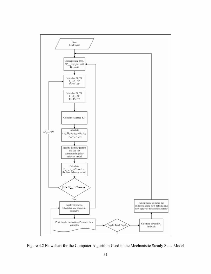
performed. Figure 4.2 shows a flow chart of the computer code used to carry out the pressure

traverse calculations. For each length increment the inclination angle is calculated from the

survey file provided or it can be input manually per the request of the user. The calculations for

both the downward flow in the drillstring and upward flow in the annulus, and flow through bit

29

nozzles are performed using the models discussed in Chapter 3. Finally fluid properties are

computed using the PVT correlations presented in Appendix A. Figure 4.2 shows the flowchart

for modeling the calculations of the mechanistic steady state model in a deviated well while

performing UBD operations.

In this model the user is required to input the following data through an EXCEL

spreadsheet.

• Injection rates (gas and drilling fluid) at surface conditions (scf/min, and GPM)

• Surface temperature and pressure (surface or choke pressure), and the geothermal

gradient.

• Survey data (measured depth, and inclination from horizontal).

• Drillstring and annular geometries. (OD, ID, hole size, pipe roughness).

• Depth at which calculations starts and either total depth or the depth at which the user

wishes to finish calculations.

• Length increment.

• Drilling fluid properties (plastic viscosity and density).

• Bit nozzle diameters.

• Formation fluid production rates (bbl/day).

4.1 Field Example

The computer program described above has been used to simulate the behavior of a

deviated well while drilling underbalanced using joint pipes with injection from the drillstring. In

order to demonstrate the validity of the model, a field case was simulated and results compared

with measurements. The field case is a previously drilled and cased well with a horizontal

30

sidetrack. Due to past history of lost circulation and the nature of the field there the decision was

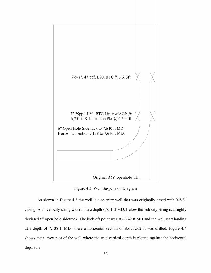
made to drill the well using UBD technique. Figure 4.3 shows the well suspension diagram.

Figure 4.1: Incremental Wellbore Calculations Path in a Deviated Wellbore

31

Figure 4.2 Flowchart for the Computer Algorithm Used in the Mechanistic Steady State Model

32

9-5/8", 47 ppf, L80, BTC@ 6,673ft

7" 29ppf, L80, BTC Liner w/ACP @6,751 ft & Liner Top Pkr @ 6,594 ft

6" Open Hole Sidetrack to 7,640 ft MD.Horizontal section 7,138 to 7,640ft MD.

Original 8 ½" openhole TD

Figure 4.3: Well Suspension Diagram

As shown in Figure 4.3 the well is a re-entry well that was originally cased with 9-5/8”

casing. A 7” velocity string was run to a depth 6,751 ft MD. Below the velocity string is a highly

deviated 6” open hole sidetrack. The kick off point was at 6,742 ft MD and the well start landing

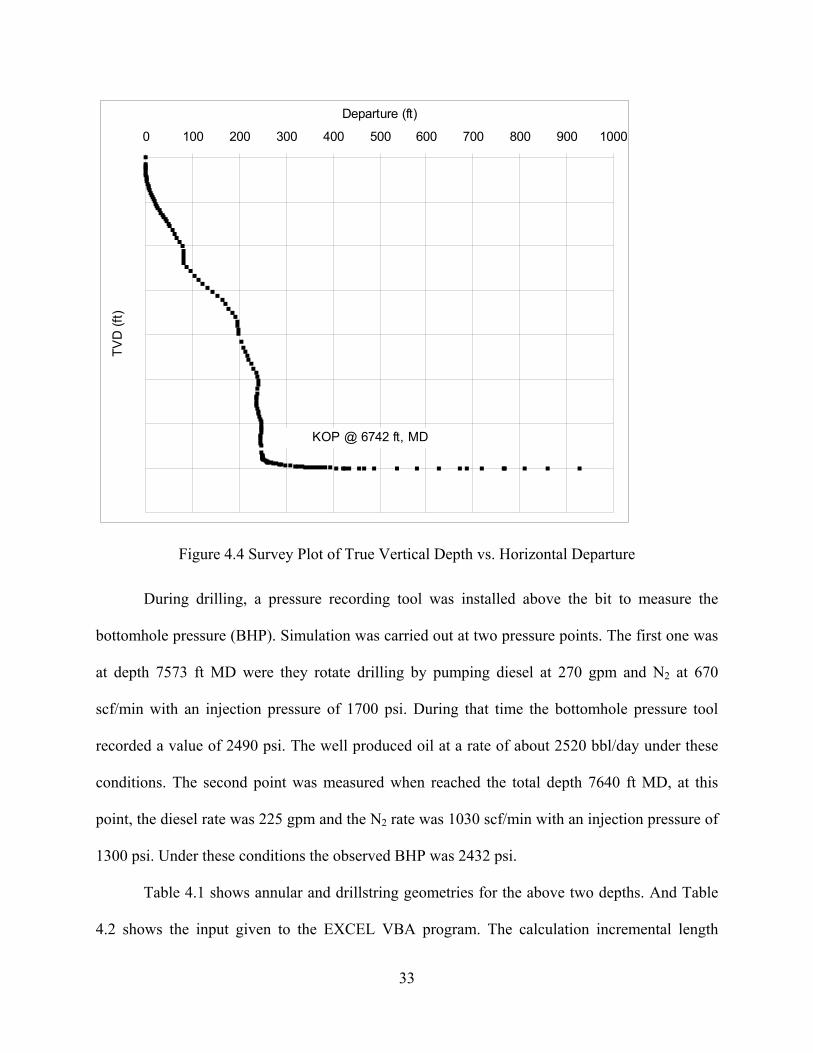
at a depth of 7,138 ft MD where a horizontal section of about 502 ft was drilled. Figure 4.4

shows the survey plot of the well where the true vertical depth is plotted against the horizontal

departure.

33

0 100 200 300 400 500 600 700 800 900 1000

Departure (ft)TV

D (f

t)

KOP @ 6742 ft, MD

Figure 4.4 Survey Plot of True Vertical Depth vs. Horizontal Departure

During drilling, a pressure recording tool was installed above the bit to measure the

bottomhole pressure (BHP). Simulation was carried out at two pressure points. The first one was

at depth 7573 ft MD were they rotate drilling by pumping diesel at 270 gpm and N2 at 670

scf/min with an injection pressure of 1700 psi. During that time the bottomhole pressure tool

recorded a value of 2490 psi. The well produced oil at a rate of about 2520 bbl/day under these

conditions. The second point was measured when reached the total depth 7640 ft MD, at this

point, the diesel rate was 225 gpm and the N2 rate was 1030 scf/min with an injection pressure of

1300 psi. Under these conditions the observed BHP was 2432 psi.

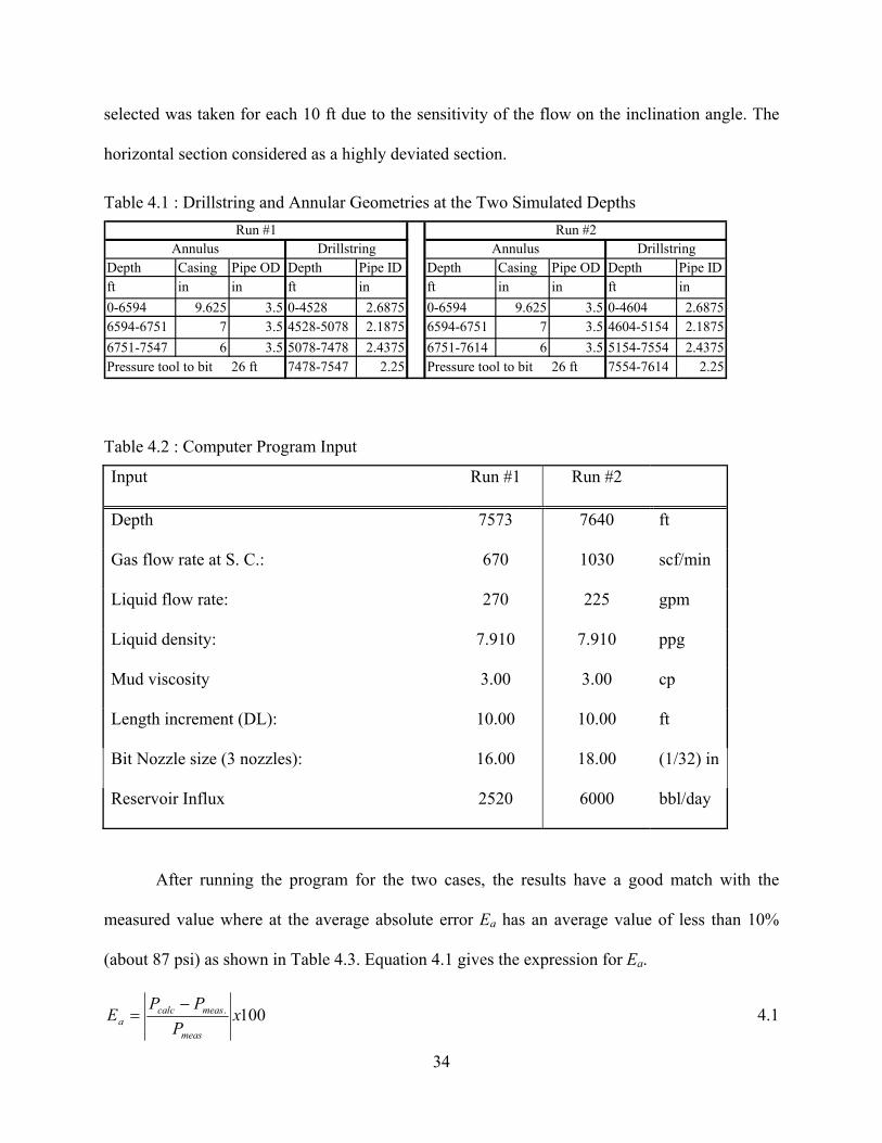
Table 4.1 shows annular and drillstring geometries for the above two depths. And Table

4.2 shows the input given to the EXCEL VBA program. The calculation incremental length

34

selected was taken for each 10 ft due to the sensitivity of the flow on the inclination angle. The

horizontal section considered as a highly deviated section.

Table 4.1 : Drillstring and Annular Geometries at the Two Simulated Depths

Depth Casing Pipe OD Depth Pipe ID Depth Casing Pipe OD Depth Pipe IDft in in ft in ft in in ft in0-6594 9.625 3.5 0-4528 2.6875 0-6594 9.625 3.5 0-4604 2.68756594-6751 7 3.5 4528-5078 2.1875 6594-6751 7 3.5 4604-5154 2.18756751-7547 6 3.5 5078-7478 2.4375 6751-7614 6 3.5 5154-7554 2.4375Pressure tool to bit 26 ft 7478-7547 2.25 Pressure tool to bit 26 ft 7554-7614 2.25

Annulus DrillstringRun #1 Run #2

Annulus Drillstring

Table 4.2 : Computer Program Input

Input Run #1 Run #2

Depth 7573 7640 ft

Gas flow rate at S. C.: 670 1030 scf/min

Liquid flow rate: 270 225 gpm

Liquid density: 7.910 7.910 ppg

Mud viscosity 3.00 3.00 cp

Length increment (DL): 10.00 10.00 ft

Bit Nozzle size (3 nozzles): 16.00 18.00 (1/32) in

Reservoir Influx 2520 6000 bbl/day

After running the program for the two cases, the results have a good match with the

measured value where at the average absolute error Ea has an average value of less than 10%

(about 87 psi) as shown in Table 4.3. Equation 4.1 gives the expression for Ea.

100. xPPP

Emeas

meascalca

−= 4.1

35

A commercial simulator was used to compare the results of this study to the simulator

output; this recent version of the simulator uses the empirical correlation that was developed by

Hasan and Kabir. Table 4.3 shows the output result of the developed model in this study with the

result of the simulator output.

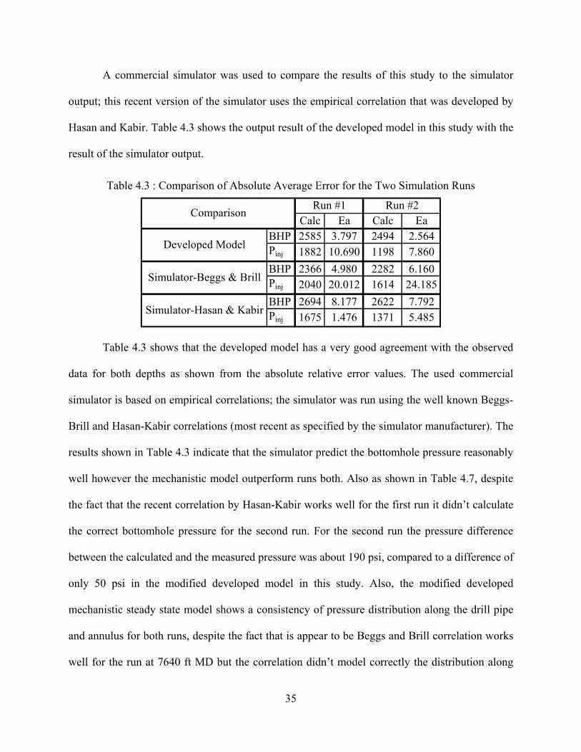
Table 4.3 : Comparison of Absolute Average Error for the Two Simulation Runs

Calc Ea Calc EaBHP 2585 3.797 2494 2.564Pinj 1882 10.690 1198 7.860BHP 2366 4.980 2282 6.160Pinj 2040 20.012 1614 24.185BHP 2694 8.177 2622 7.792Pinj 1675 1.476 1371 5.485

Comparison

Developed Model

Run #2Run #1

Simulator-Beggs & Brill

Simulator-Hasan & Kabir

Table 4.3 shows that the developed model has a very good agreement with the observed

data for both depths as shown from the absolute relative error values. The used commercial

simulator is based on empirical correlations; the simulator was run using the well known Beggs-

Brill and Hasan-Kabir correlations (most recent as specified by the simulator manufacturer). The

results shown in Table 4.3 indicate that the simulator predict the bottomhole pressure reasonably

well however the mechanistic model outperform runs both. Also as shown in Table 4.7, despite

the fact that the recent correlation by Hasan-Kabir works well for the first run it didn’t calculate

the correct bottomhole pressure for the second run. For the second run the pressure difference

between the calculated and the measured pressure was about 190 psi, compared to a difference of

only 50 psi in the modified developed model in this study. Also, the modified developed

mechanistic steady state model shows a consistency of pressure distribution along the drill pipe

and annulus for both runs, despite the fact that is appear to be Beggs and Brill correlation works

well for the run at 7640 ft MD but the correlation didn’t model correctly the distribution along

36

the wellbore and gave a large injection pressure. In addition, the use of different mechanistic

models shows that they can capture the behavior of the flow during different combination of

flow rates and pipe geometries, unlike the empirical correlations where they reported not to work

well in oil field cases, and also they were developed by production engineers to handle either

upward flow during the pipe or the annulus. Another reason why such large error occurred is the

fact that this well has a large horizontal section which is this case was treated as highly deviated;

hence the calculations may be affected by this assumption.

Run #1

0

1000

2000

3000

4000

5000

6000

7000

8000

0 500 1000 1500 2000 2500 3000 3500

Pressure (psi)

Dep

th, M

D (f

t)

Hasan-Kabir Beggs-BrillDeveloped Model Observed Points

Run #2

0

1000

2000

3000

4000

5000

6000

7000

8000

9000

0 500 1000 1500 2000 2500 3000 3500

Pressure (psi)

Dep

th, M

D (f

t)

Hasan-Kabir Beggs-BrillDeveloped Model Observed Points

Figure 4.5: Comparison between Field Measurements and Simulators Output at Both Runs

37

Figure 4.5 shows a plot of the two simulators results with the measured data for both

simulated depths. The effect of inclination is seen thoroughly in the developed model whereas

the commercial simulator shows changes in the geometry where it will effect the flow behavior.

Also the combination use of mechanistic steady state models has eliminated any sharp transition

in the calculations, which is not the same case for commercial simulator output.

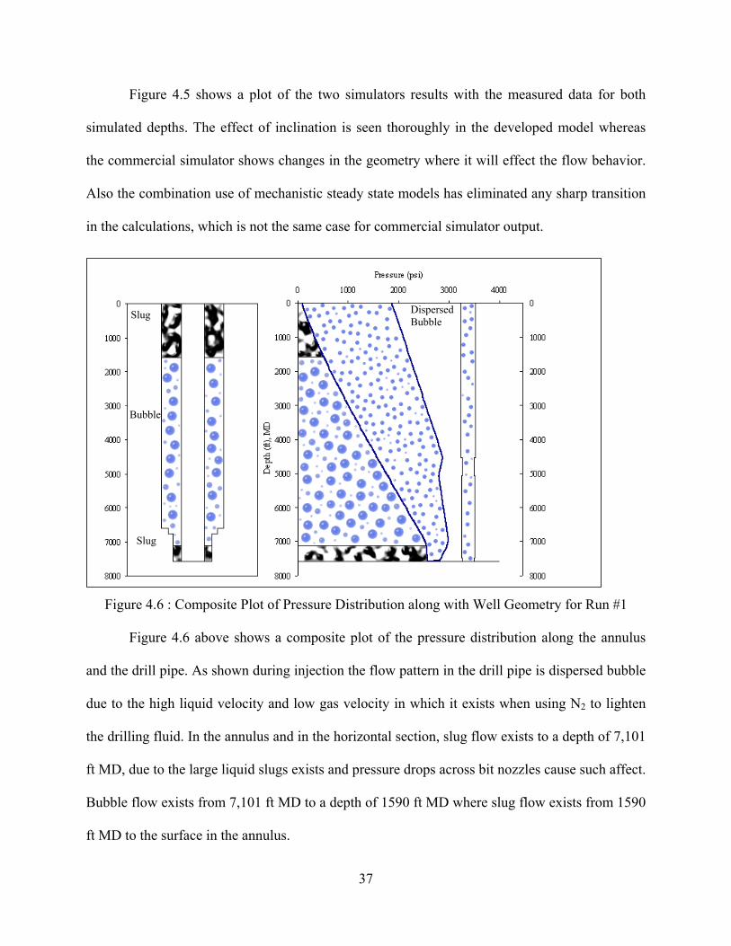
Figure 4.6 : Composite Plot of Pressure Distribution along with Well Geometry for Run #1

Figure 4.6 above shows a composite plot of the pressure distribution along the annulus

and the drill pipe. As shown during injection the flow pattern in the drill pipe is dispersed bubble

due to the high liquid velocity and low gas velocity in which it exists when using N2 to lighten

the drilling fluid. In the annulus and in the horizontal section, slug flow exists to a depth of 7,101

ft MD, due to the large liquid slugs exists and pressure drops across bit nozzles cause such affect.

Bubble flow exists from 7,101 ft MD to a depth of 1590 ft MD where slug flow exists from 1590

ft MD to the surface in the annulus.

Dispersed Bubble

Slug

Bubble

Slug

38

-

1,000

2,000

3,000

4,000

5,000

6,000

7,000

8,000

0 0.2 0.4 0.6 0.8 1

∆P/∆L, Liquid holdup

-

1,000

2,000

3,000

4,000

5,000

6,000

7,000

8,000

0 20 40 60 80 100

Inclination (Deg)

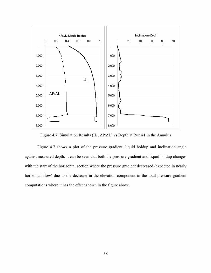
Figure 4.7: Simulation Results (HL, ∆P/∆L) vs Depth at Run #1 in the Annulus

Figure 4.7 shows a plot of the pressure gradient, liquid holdup and inclination angle

against measured depth. It can be seen that both the pressure gradient and liquid holdup changes

with the start of the horizontal section where the pressure gradient decreased (expected in nearly

horizontal flow) due to the decrease in the elevation component in the total pressure gradient

computations where it has the effect shown in the figure above.

HL

∆P/∆L

39

Chapter 5

Conclusion and Recommendations

5.1 Conclusions

• The use of mechanistic steady state model has proven to give better prediction than

empirical correlations especially when trying to design UBD operation within a pressure

window.

• The developed model and the computer program is only valid to steady-state conditions.

• The combination of flow prediction and flow behavior models has proven to effectively

predict flow profile in a steady state condition.

• The development of the computer program in EXCEL VBA® will ease both its use and

further development.

• The program can be used in spreadsheet calculations to carry several models and

predictions.

• The use of the marching algorithm is recommended taking into account selection of the

appropriate length increment since if the survey data was taken alone this will have an

increase effect on the calculations. Also a simple interpolation is used in order to find the

inclination angle from the horizontal at each given depth.

• The bit model used has proven to work in estimating injection pipe pressure as shown

between the comparison between the results of the simulator and the developed model in

this study.

40

• This program can be used also to calculate the pressure drop in conditions other and than

UBD operations. However, some modifications are needed in order to accommodate for

variables fluid influx from the reservoir.

• This tool can be used as a design tool where UBD controlled surface parameters such as

injection rates and choke pressures are calculated in order to drill the reservoir within the

desired UBD window required by the first design of the UBD operation.

• It is shown in the field example calculations that the assumptions of highly deviated wells

have affected the calculations but not as large as when using the correlations.

5.2 Recommendations

• Any future development of mechanistic models should improve results by increasing

accuracy in liquid holdup and pressure gradient predictions.

• Developing a model for a truly horizontal increment are recommended also to enhance

the calculations and create a unified model for all angle ranges.

• The developed model can be coupled with the time dependent model developed by Perez-

Tellez31 and find an un-steady state solution for deviated wellbores drilled under UBD

conditions. This will allow analysis of the well during pipe connections.

41

REFERENCES

1 Gas Research Institute (GRI), Underbalanced Drilling Manual, published by Gas Research Institute, Chicago, Illinois, 1997.

2 Bennion D.B and Thomas F.B.: “Underbalanced Drilling of Horizontal Wells: Does It

Really Eliminate Formation Damage?” paper 27352 presented at the SPE Intl. Symposium on Formation Damage Control held in Lafayette, Louisiana, February 7-10, 1994.

3 Guo, B, Hareland G., and Rajtar, J.: “Computer Simulation Predicts Unfavorable Mud

Rate for Aerated Mud Drilling”, paper SPE 26892 presented at the 1993 SPE Eastern Regional Conferences held in Pittsburgh, Pa. Nov. 2-4 1993.

4 Liu, G. and Medley, G.H.: “Foam Computer Model Helps in Analysis of Underbalanced

Drilling”, Oil and Gas J. July 1,1996.

5 Beggs, H.D. and Brill, J.P.: “A Study of Two phase Flow in Inclined Pipes”, JPT. May 1973. pp. 607-617.

6 Maurer Engineering Inc.: Underbalanced Drilling and Completion Manual, copyrighted

1998, DEA-101, Houston, Texas.

7 Maurer Engineering Inc.: Air/Mist/Foam/ Hydraulics Model, User’s Manual, copyrighted 1998, DEA-101, Houston, Texas.

8 Tian, S., Medley G.H. Jr., and Stone, C.R.: “Optimizing Circulation While Drilling

Underbalanced”, World Oil, June 2000, pp 48-55.

9 Tian, S., Medley G.H. Jr.: “Re-evaluating Hole Cleaning in Underbalanced Drilling Applications”, paper presented at the IADC Underbalanced Drilling Conference and Exhibitions, Houston, Texas, August 28-29 2000.

10 Bijleveld, A.F., Koper, M., and Saponja, J.: “Development and Application of an

Underbalanced Drilling Simulator”, paper IADC/SPE 39303 presented at the 1996 IADC/SPE Drilling Conferences held in Dallas, Texas, March 3-6, 1996.

11 Ansari, A.M., Sylvester, N.D., Sarica, C., Shoham, O., and Brill, J.P.: “A Comprehensive

Mechanistic Model for Upward Two Phase Flow in Well bores,” SPE Production and Facil., p. 143, May (1994).

12 Gomez, L., Shoham, O., Schmidt, Z., Chokshi, R., Brown, A., and Northug, T.: “A

Unified Mechanistic Model for Steady-State Two phase Flow in Wellbores and Pipelines,” paper SPE 56520 presented at the 1999 ATCE Houston, Texas, October 3-6, 1999.

42

13 Kaya, A.S., Sarica, C., and Brill, J.P.: “Comprehensive Mechanistic Modeling of Two phase Flow in Deviated Wells,” paper SPE 56522 presented at the 1999 Annual and Technical Conferences and Exhibition, Houston, TX, October 3-6, 1999.

14 Caetano, E.F., Shoham, O., and Brill, J.P.: “Upward Vertical Two phase Flow Through

Annulus Part I: Single-Phase Friction Factor, Taylor Bubble Rise Velocity, and Flow Pattern Prediction,” Journal of Energy Resources Technology (1992) 114, 1.

15 Caetano, E.F., Shoham, O., and Brill, J.P.: “Upward Vertical Two phase Flow Through

Annulus Part II: Modeling Bubble, Slug, and Annular Flow,” Journal of Energy Resources Technology (1992) 114, 14.

16 Hasan, A.R. and Kabir, C.S: “Tow-Phase Flow in Vertical and Inclined Annuli,” Intl. J.

Multiphase Flow (1992) 18, 279.

17 Lage, A.C.V.M and Timer.: “Mechanistic Model for Upward Tow-Phase Flow in Annuli,” paper 63127, presented at the 2000 SPE ATCE help in Dallas, Texas, October 1-4, 2000.

18 Perez-Téllez, C., Smith, J.R., and Edwards, J.K.: “A New Comprehensive, Mechanistic

Model for Underbalanced Drilling Improves Wellbore Pressure Predictions”, paper SPE 74426 presented at the 2002 IPCEM held in Villahermosa, Mexico, February 10-12, 2002.

19 Gavignet, A.A., and Sobey, I.J.: “A Model for The Transport of Cuttings in Highly

Deviated Wells,” paper 15417, presented at the 1986 SPE ATCE held in New Orleans, Louisiana, October 5-8, 1986.

20 Brown, N.P., Bern, P.A., and Weaver, A.: “Cleaning Deviated Holes: New Experimental

and Theoretical Studies,” paper 18636, presented at the 1986 SPE/IADC conference held in New Orleans, Louisiana, February.

21 Brill, J.P. and Mukherjee, H.: Multiphase Flow in Wells, Monograph Volume 17

copyright 1999 by the Society of Petroleum Engineers Inc.

22 Beggs, H.D.: Production Optimization Using Nodal Analysis, OGCI publications, Oil and Gas Consultants International Inc. Tulsa, OK, 1991.

23 Taitel, Y., Barnea, D. and Duckler, A.E.: “Modeling Flow Pattern Transitions for Steady

Upward Gas-Liquid Flow in Vertical Tubes”, AIChE J. (1980) 26, pp 345-354.

24 Hasan, A.R.: “Void Fraction in Bubbly and Slug Flow in Downward Vertical and Inclined Systems”, paper SPE 26522, presented at 1993 Annual Technical Conference and Exhibition held in Houston, TX, October 3-6, 1993.

43

25 Hasan, A.R.: “Inclined Two phase Flow: Flow Pattern, Void Fraction and Pressure Drop in Bubbly, Slug and Churn Flow,” Particulate Phenomena and Multiphase Transport, Hemisphere Publishing Corp., New York city (1988), 229.

26 Hasan, A.R. and Kabir, C.S.: “Predicting Multiphase Flow Behavior in a Deviated Well,”

SPEDE (Nov, 1988), 474.

27 Harmathy, T.Z.: “Velocity of Large Drops and Bubbles in Media of Infinite or Restricted Extent,” AIChE J. (1960) 6, 281-288.

28 Zuber, N. and Findlay, J.A.: “Average Volumetric Concentration in Two Phase Flow

System”, Journal of Heat Transfer, pages 453-468, November 1965.

29 Alves, I. N.: Slug Flow Phenomena in Inclined Pipes, Ph.D. Dissertation, The University of Tulsa, Tulsa, Oklahoma, 1991.

30 Wallis, G.B.: One Dimensional Two phase Flow, McGraw-Hill (1969).

31 Perez-Tellez, C.: Improved Bottomhole Pressure Control for Underbalanced Drilling Operations, Ph.D Dissertation, Louisiana State University (2002).

32 Tengesdal, J.O., Kaya, A.S., and Cem Sarica.: “Flow Pattern Transition and

Hydrodynamic Modeling of Churn Flow,” SPE J (December 1999) 4, No. 4, pp 342-348.

33 Colebrook, C.F.: “Turbulent Flow in Pipes With Particular Reference to the Transition Region Between the Smooth and Rough Pipe Laws,” J. Inst. Civil Eng. (1939), 11, 133.

34 Gunn, D.J. and Darling, C.W.W.: “Fluid Flow and Energy Losses in Non Circular

Conduits,” Trans. AIChE (1963) 41, 163.

35 Taitel, Y. nd Barnea, D.: “Counter Current Gas-Liquid Vertical Flow, Model for Flow Pattern and Pressure Drop,” Int. J. Multiphase Flow (1983) 9, 637-647.

36 Alves, I. N., Caetano, E. F., Minami, K. and Shoham, O.: "Modeling Annular Flow

Behavior for Gas Wells," SPE Production Engineering, (November 1991), 435-440

37 Henstock, W.H. and Hanratty, T.J.: “The Interfacial Drag and the Height of the Wall Layer in Annular Flow”, AIChE J., 22, No. 6, (Nov. 1976),990-1000.

38 Wallis, G.B.: One Dimensional Two phase Flow, McGraw-Hill (1969).

39 Bourgoyne, A.T. Jr., Chenevert M.E., Millheim, K.K., and Young, F.S.: Applied Drilling

Engineering, SPE textbook series, 1984.

40 Dranchuk, P.M., and Abu-Kassem, J.H.: “Calculations of Z-Factors for Natural Gases Using Equation of State,” J. Canadian Pet. Tech. (July-Sep 1975)14, 34

44

41 Standing, M.B., and Katz, D.L.: “Density of Natural Gases,” Trans. ,AIME (1942) 146, 140

42 Lee, A.L., et al.: “The Viscosity of Natural Gases,” JPT, Aug., 1966.

43 Beggs, H. D. and Robinson, J. R.: “Estimating the Viscosity of Crude Oil Systems,” JPT,

Sept, 1959.

45

Appendix A: PVT Correlations

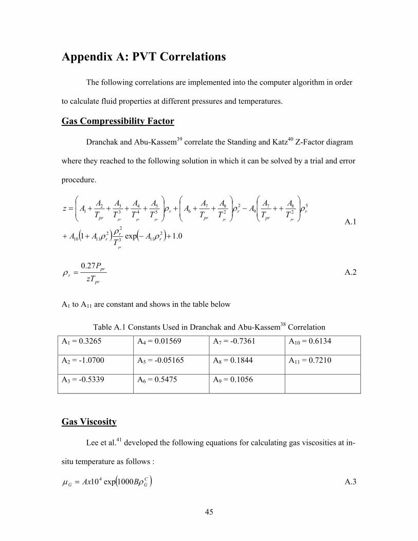
The following correlations are implemented into the computer algorithm in order

to calculate fluid properties at different pressures and temperatures.

Gas Compressibility Factor

Dranchak and Abu-Kassem39 correlate the Standing and Katz40 Z-Factor diagram

where they reached to the following solution in which it can be solved by a trial and error

procedure.

( ) ( ) 0.1exp1 2113

22

1110

5287

92

287

655

44

332

1

+−++

++−

+++

++++=

rr

r

rpr

rpr

rpr

AT

AA

TA

TAA

TA

TAA

TA

TA

TA

TAAz

pr

prprprprpr

ρρρ

ρρρ

A.1

pr

prr zT

P27.0=ρ A.2

A1 to A11 are constant and shows in the table below

Table A.1 Constants Used in Dranchak and Abu-Kassem38 Correlation

A1 = 0.3265 A4 = 0.01569 A7 = -0.7361 A10 = 0.6134

A2 = -1.0700 A5 = -0.05165 A8 = 0.1844 A11 = 0.7210

A3 = -0.5339 A6 = 0.5475 A9 = 0.1056

Gas Viscosity

Lee et al.41 developed the following equations for calculating gas viscosities at in-

situ temperature as follows :

( )CGG BAx ρµ 1000exp104= A.3

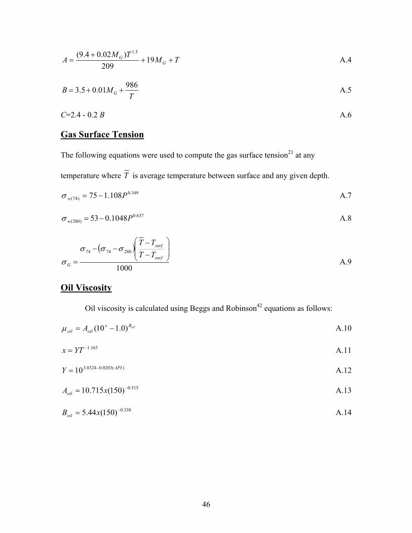
46

TMTM

A GG ++

+= 19

209)02.04.9( 5.1

A.4

TMB G

98601.05.3 ++= A.5

C=2.4 - 0.2 B A.6

Gas Surface Tension

The following equations were used to compute the gas surface tension21 at any

temperature where T is average temperature between surface and any given depth.

349.0)74( 108.175 Pw −=σ A.7

637.0)280( 1048.053 Pw −=σ A.8

( )

1000

2807474

−−

−−

=surf

surf

G

TTTT

σσσ

σ A.9

Oil Viscosity

Oil viscosity is calculated using Beggs and Robinson42 equations as follows:

oilBxoiloil A )0.110( −=µ A.10

163.1−= YTx A.11

)(0203.00324.310 APIY −= A.12

515.0)150(715.10 −= xAoil A.13

338.0)150(44.5 −= xBoil A.14

47

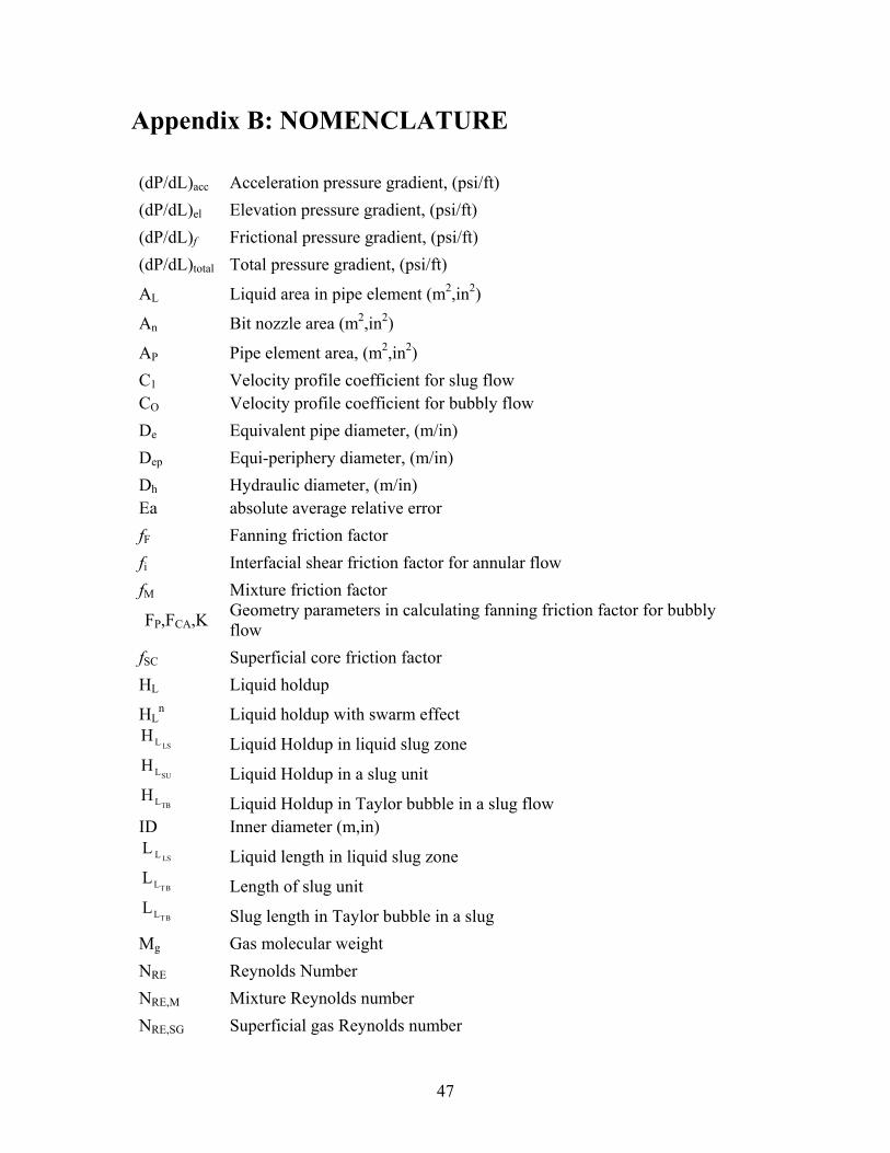
Appendix B: NOMENCLATURE

(dP/dL)acc Acceleration pressure gradient, (psi/ft) (dP/dL)el Elevation pressure gradient, (psi/ft) (dP/dL)f Frictional pressure gradient, (psi/ft) (dP/dL)total Total pressure gradient, (psi/ft)

AL Liquid area in pipe element (m2,in2)

An Bit nozzle area (m2,in2)

AP Pipe element area, (m2,in2) C1 Velocity profile coefficient for slug flow CO Velocity profile coefficient for bubbly flow De Equivalent pipe diameter, (m/in) Dep Equi-periphery diameter, (m/in) Dh Hydraulic diameter, (m/in) Ea absolute average relative error fF Fanning friction factor fi Interfacial shear friction factor for annular flow fM Mixture friction factor

FP,FCA,K Geometry parameters in calculating fanning friction factor for bubbly flow

fSC Superficial core friction factor HL Liquid holdup

HLn Liquid holdup with swarm effect

LSLH Liquid Holdup in liquid slug zone

SULH Liquid Holdup in a slug unit

TBLH Liquid Holdup in Taylor bubble in a slug flow

ID Inner diameter (m,in) LSLL

Liquid length in liquid slug zone TBLL

Length of slug unit TBLL

Slug length in Taylor bubble in a slug Mg Gas molecular weight NRE Reynolds Number NRE,M Mixture Reynolds number NRE,SG Superficial gas Reynolds number

48

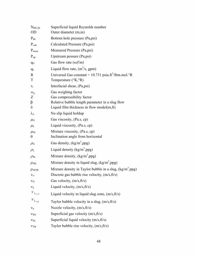
NRE,SL Superficial liquid Reynolds number OD Outer diameter (m,in) Pbh Bottom hole pressure (Pa,psi) Pcalc Calculated Pressure (Pa,psi) Pmeas Measured Pressure (Pa,psi) Pup Upstream pessure (Pa,psi) qG Gas flow rate (scf/m)

qL Liquid flow rate, (m3/s, gpm) R Universal Gas constant = 10.731 psia.ft3/lbm.mol.°R T Temperature (°K,°R) τi Interfacial shear, (Pa,psi) wg Gas weighing factor Z Gas compressibility factor β Relative bubble length parameter in a slug flow δ Liquid film thickness in flow model(m,ft) λL No slip liquid holdup µG Gas viscosity, (Pa.s, cp) µL Liquid viscosity, (Pa.s, cp) µM Mixture viscosity, (Pa.s, cp) θ Inclination angle from horizontal

ρG Gas density, (kg/m3,ppg)

ρL Liquid density (kg/m3,ppg)

ρM Mixture density, (kg/m3,ppg)

ρΜL Mixture density in liquid slug, (kg/m3,ppg)

ρΜTB Mixture density in Taylor bubble in a slug, (kg/m3,ppg) ν∞ Discrete gas bubble rise velocity, (m/s,ft/s) νG Gas velocity, (m/s,ft/s) νL Liquid velocity, (m/s,ft/s)

L SLv Liquid velocity in liquid slug zone, (m/s,ft/s)

T BLv Taylor bubble velocity in a slug, (m/s,ft/s)

νn Nozzle velocity, (m/s,ft/s) νSG Superficial gas velocity (m/s,ft/s) νSL Superficial liquid velocity (m/s,ft/s) νTB Taylor bubble rise velocity, (m/s,ft/s)

49

VITA

Faisal Abdullah ALAdwani Born in Kuwait city, Kuwait, in October 10, 1975. In January

1998, he received a degree Bachelor of Science in Petroleum Engineering from Kuwait

University. In March 1998, he joined Kuwait Foreign Petroleum Exploration Company where he

worked as a petroleum engineer and was assigned to field operations in the Southeast Asia

Region. In August 2001, he joined the Craft & Hawkins Petroleum Engineering Department at

Louisiana State University to work towards a Master of Science in Petroleum Engineering. He is

a member of the Society of Petroleum Engineers.