Application of model based post-stack inversion in the

Application of model based post-stack inversionin the characterization of reservoir sands containingporous, tight and mixed facies: A case studyfrom the Central Indus Basin, Pakistan

MUHAMMAD TOQEER1, AAMIR ALI

1,* , TIAGO M ALVES2, ASHAR KHAN

1,ZUBAIR

3 and MATLOOB HUSSAIN1

1Department of Earth Sciences, Quaid-i-Azam University, Islamabad 45320, Pakistan.

23D Seismic Lab, School of Earth and Ocean Sciences, CardiA University, CardiA CF10 3AT, UK.

3Software Integrated Solutions, Schlumberger, Pakistan.*Corresponding author. e-mail: [email protected] [email protected]

MS received 7 May 2020; revised 1 November 2020; accepted 10 November 2020

Porosity is a key parameter for reservoir evaluation. Inferring the porosity from seismic data is oftenchallenging and prone to uncertainties due to number of factors. The main aim of this paper is to show theapplicability of seismic inversion on old vintage seismic data to map spatial porosity at reservoir level.3D-seismic and wireline log data are used to map the reservoir properties of the Lower Goru productivesands in the Gambat Latif block, Central Indus Basin, Pakistan. The Lower Goru formation was inter-preted with the help of seismic and well data. Interpreted horizons are thus further used in model-basedseismic inversion techniques to map the spatial distribution of porosity. Well-log data are used in theconstruction of low acoustic impedance models. Calibration of reservoir porosity with inverted acousticimpedance is achieved through well-log data. The results from model-based inversion reasonably estimatethe porosity distribution within the C-sand interval of the Lower Goru Member. After post-stackinversion, the porosity values at wells Tajjal-01, Tajjal-02 and Tajjal-03 are 10%, 8% and 12%, respec-tively. Porosity values calculated from post-stack inversion at the corresponding well locations are in goodagreement with the borehole-derived porosity.

Keywords. Indus basin; post-stack inversion; model-based inversion; reservoir modelling.

1. Introduction

Reservoir characterization comprises the estima-tion of key reservoir properties such as porosity,permeability, upper and lower reservoir bound-aries, their lateral and vertical extent, hetero-geneity, and type and volume of subsurface Cuids(Avseth et al. 2005; Bacon et al. 2007). Seismic andwell-log data are typically used to estimate reser-voir properties at different scale(s) of investigation

(Chen and Sidney 1997; Lindseth 1979; King 1990;Hearts et al. 2002; Chopra and Marfurt 2007).Interpolations and other geostatistical techniquesalso help to eDciently link seismic, well-log, coredata to Beld observations, improving our under-standing of the local geology (Caers et al. 2001;Mukerji et al. 2001; Walls et al. 2004; Bosch et al.2010; Azevedo et al. 2017).Seismic inversion techniques are used to retrieve

acoustic impedance from seismic reCection proBles

J. Earth Syst. Sci. (2021) 130:61 � Indian Academy of Scienceshttps://doi.org/10.1007/s12040-020-01543-5 (0123456789().,-volV)(0123456789().,-volV)

and 3D volumes, spatial distribution of deposi-tional facies, local petrophysical properties anddistinct reservoir parameters (Angeleri and Carpi1982; Yao and Gan 2000; Walls et al. 2004; Boschet al. 2009; Grana and Dvorkin 2011). Seismic,well-log and inversion data are later combined toderive the different physical parameters (i.e.,porosity and lithological information) of keyreservoir intervals (Landa et al. 2000; Yao and Gan2000; Leite and Vidal 2011; Simm and Bacon2014).The beneBts of seismic inversion include an

improved seismic resolution (Delaplanche et al.1982), and better seismic interpretation owing tothe fact that layer-oriented impedance displaysmore complete constraints for reservoir models(Ashcroft 2011). For post-stack data, the maininversion techniques are sparse-spike, model-basedand coloured inversion, which are based on differ-ent algorithms (Silva et al. 2004; Veeken and Silva2004; Veeken and Rauch-Davies 2006; Veeken2007; Ashcroft 2011; Wang 2017).Post-stack seismic inversion methods utilize

post-stack seismic data. Appropriate processingparameters are required for amplitude and phasepreservation with higher signal-to-noise ratios(Simm and Bacon 2014). Filtered lower frequenciesin the processed data should be compensated byincorporating low frequency models for inversion(Sams and Carter 2017). Likewise, the absence ofhigher frequencies due to absorption should also beconsidered (Vecken and Da Silva 2004). Due to theband-limited nature of post-stack seismic data, theabsence of higher and lower frequencies may resultin ambiguities when resolving thin beds and esti-mating local elastic properties (Zhang et al. 2012;Rosa 2018). Nevertheless, despite the inherentlimitations of post-stack inversion techniques, theirapplicability and popularity are growing for arange of geophysical and geological studies (Li2014; Verma et al. 2018; Gogoi and Chatterjee2019; Singha et al. 2019; Teixeira and Maul 2020).Seismic inversion techniques are often applied in

the different basins worldwide to Bnd the acousticimpedance and reservoir parameters (Alavi 2004;Leite and Vidal 2011). In several Asian basinsseismic inversion techniques have been successfullyapplied to characterize hydrocarbon bearing strata(Karbalaali et al. 2013; Sinha and Mohanty 2015;Kumar et al. 2016; Das et al. 2017; Iravani et al.2017; Jafari et al. 2017).Owing to its hydrocarbon potential, the Indus

basin has been extensively studied since the 1930’s

(de Terra et al. 1936; Williams 1959; Quadri 1986;Zaigham and Mallick 2000). The presence of theLower Goru Formation, a proven reservoir, hasbeen demonstrated in the region. However,important variations in the thickness and reservoirproperties of the Lower Goru Formation are alsoreported within the Indus Basin (Khattak et al.1999).The aim of this paper is to map the spatial

porosity of a reservoir interval using a limiteddataset. Old vintage 3D-seismic data are used toaccomplish this task. Certain uncertainties associ-ated with porosity estimation include the inherentlimitation of seismic techniques, i.e., seismic reso-lution, applied seismic data processing algorithms,limitations of seismic inversion techniques them-selves, and the seismic character of the local geol-ogy. The only control points are the sparse welldata used to validate the inversion process. Theresults thus obtained are subjective to discussionand criticism, but the inversion process we presentleads to the best results when compared to all theavailable techniques.Seismic data was used to map key seismic-

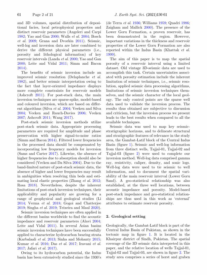
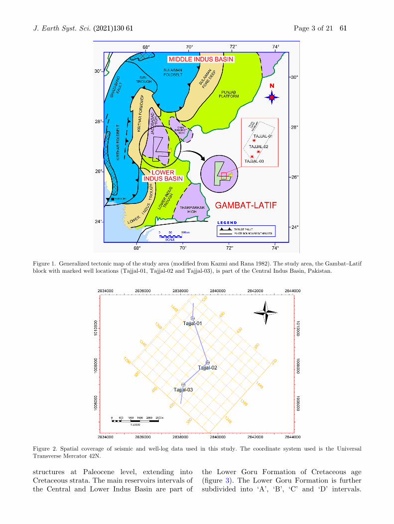
stratigraphic horizons, and to delineate structuraland stratigraphic features of relevance in the studyarea, the Gambat-Latif block of the Central IndusBasin (Bgure 1). Seismic and well-log informationfrom three distinct wells, Tajjal-01, Tajjal-02 andTajjal-03 (Bgure 2) were used to complete ourinversion method. Well-log data comprised gammaray, resistivity, caliper, density, and sonic logs.Well-log data were used to tie seismic to wellinformation, and to document the spatial vari-ability of the main reservoir interval (Lower GoruSand). A geo-statistical relationship was alsoestablished, at the three well locations, betweenacoustic impedance and porosity. Model-basedpost-stack impedance and geo-statistical relation-ships are thus used in this work as ‘external’attributes to estimate reservoir porosity.

2. Geological setting

Geologically, the Gambat-Latif block is part of theCentral Indus Basin of Pakistan, as shown in thetectonic map in Bgure 1. It is located in theKhairpur district of Sindh, Pakistan. The spatialcoverage of the 3D seismic data interpreted in thispaper, and the relative location of wells Tajjal-01,Tajjal-02 and Tajjal-03, are shown in Bgure 2. Thestudy area comprises a series of horst and graben

61 Page 2 of 21 J. Earth Syst. Sci. (2021) 130:61

structures at Paleocene level, extending intoCretaceous strata. The main reservoirs intervals ofthe Central and Lower Indus Basin are part of

the Lower Goru Formation of Cretaceous age(Bgure 3). The Lower Goru Formation is furthersubdivided into ‘A’, ‘B’, ‘C’ and ‘D’ intervals.

Figure 1. Generalized tectonic map of the study area (modiBed from Kazmi and Rana 1982). The study area, the Gambat–Latifblock with marked well locations (Tajjal-01, Tajjal-02 and Tajjal-03), is part of the Central Indus Basin, Pakistan.

Figure 2. Spatial coverage of seismic and well-log data used in this study. The coordinate system used is the UniversalTransverse Mercator 42N.

J. Earth Syst. Sci. (2021) 130:61 Page 3 of 21 61

These sandy intervals are proven reservoirs(Ahmed et al. 2004), and are limited to the east andwest by regional NW-trending extensional faults(Kazmi and Abbasi 2008).A regional stratigraphic chart for the Central

and Lower Indus Basins is displayed in Bgure 3.The Cretaceous stratigraphic succession comprisesthe Sembar, Goru, Parh, MoghalKot, Fort Munroand Pab Formations (Afzal et al. 2009; Abbasiet al. 2016). The Sembar Formation is a provensource rock throughout the Indus Basin (Robisonet al. 1999; Wandrey et al. 2004; Aziz et al. 2018).In addition, the Intra Lower Goru shales of Cre-taceous age have shown secondary, but important,source potential (Wandrey et al. 2004).Depositional environments, diagenetic changes,

shale intercalations and shale distribution stylesare key factors generating reservoir heterogeneitywithin the Lower Goru Formation (Berger et al.2009; Ali et al. 2016). Hence, reservoir properties inthe Lower Goru Formation have been estimatedin the published literature using a multitude oftechniques, from detailed structural/stratigraphic

interpretation (Akhter et al. 2015), to rock physicsmodelling (Azeem et al. 2017; Toqeer and Ali2017), AVA analyses (Ali et al. 2016; Anwer et al.2017) and seismic inversions (Ali et al. 2018).

3. Methodology

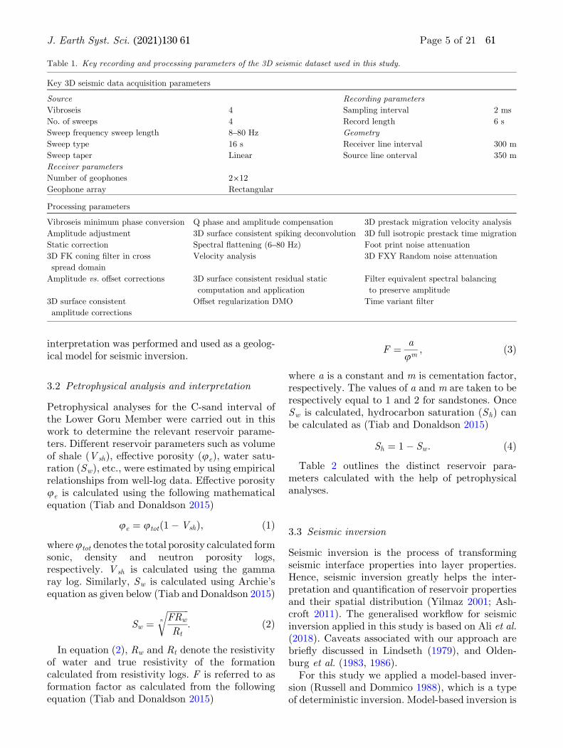
For this study only 3D seismic and well-log dataare available. 3D seismic data was acquired during2005 by BGP International via a Vibroseis sourcefor data acquisition. The processed 3D data set hasa bin spacing of 25925 m, with sampling at 2 msand a dominant frequency of 35 Hz at reservoirlevel. The processed 3D seismic data are time-migrated and zero-phased. The acquisition andprocessing parameters are outlined in the table 1.Well-log data from three wells are used in this

work. These wells were drilled to variable totaldepths in the years 2007–2008. The total drilleddepth of Tajjal-01 is 4506 m, Tajjal-02 is 3836 mand Tajjal-03 well is 3800 m, respectively. OnlyTajjal-01 well is producing gas at present, whileTajjal-02 and Tajjal-03 are reported suspended andabandoned. Prior to well-log data analysis thequality of data was checked based on the analysisof their calliper logs. The necessary correctionswere made prior the successive calculations. Themethodology can be divided into three parts. Acomprehensive summary of main steps involved inthis study is given as follows.

3.1 Seismic interpretation

Seismic interpretation is the starting point inreservoir characterization (Simm and Bacon 2014).It is paramount to tie well to seismic information tocorrectly interpret any relevant stratigraphic hori-zons. A well tie not only correlates the geology withseismic data but also assists zero-phase checking,horizon identiBcation and wavelet extraction,amongst other parameters (White 2003; Bacon et al.2007; Simm and Bacon 2014; Liner 2016). For thesereasons, synthetic seismograms were produced inthis work by convolving reCectivity from the digi-tised acoustic and density logs from well Tajjal-01with the extracted seismic wavelet. The resultingsynthetic seismogram is correlated with seismicinline 1459 at the exact location of the Tajjal-01 well(Bgure 4). In addition, horizon picking, and faultinterpretation helped to characterize the spatialdistribution of horizons and structural features inthe study area (Bgure 5). In this work, the 3D seismic

Figure 3. SimpliBed stratigraphic chart for the Lower IndusBasin. The studied reservoir interval (C-sand) is part of theLower Goru Formation, which is Early Cretaceous in age.Stratigraphic chart is modiBed from Abbasi et al. (2016).


interpretation was performed and used as a geolog-ical model for seismic inversion.

3.2 Petrophysical analysis and interpretation

Petrophysical analyses for the C-sand interval ofthe Lower Goru Member were carried out in thiswork to determine the relevant reservoir parame-ters. Different reservoir parameters such as volumeof shale (Vsh), eAective porosity (ue), water satu-ration (Sw), etc., were estimated by using empiricalrelationships from well-log data. EAective porosityue is calculated using the following mathematicalequation (Tiab and Donaldson 2015)

ue ¼ utot 1� Vshð Þ; ð1Þ

whereutot denotes the total porosity calculated formsonic, density and neutron porosity logs,respectively. Vsh is calculated using the gammaray log. Similarly, Sw is calculated using Archie’sequation as given below (Tiab and Donaldson 2015)

Sw ¼ffiffiffiffiffiffiffiffiffiffi

FRw

Rt

n

r

: ð2Þ

In equation (2), Rw and Rt denote the resistivityof water and true resistivity of the formationcalculated from resistivity logs. F is referred to asformation factor as calculated from the followingequation (Tiab and Donaldson 2015)

F ¼ a

um; ð3Þ

where a is a constant and m is cementation factor,respectively. The values of a and m are taken to berespectively equal to 1 and 2 for sandstones. OnceSw is calculated, hydrocarbon saturation (Sh) canbe calculated as (Tiab and Donaldson 2015)

Sh ¼ 1� Sw: ð4Þ

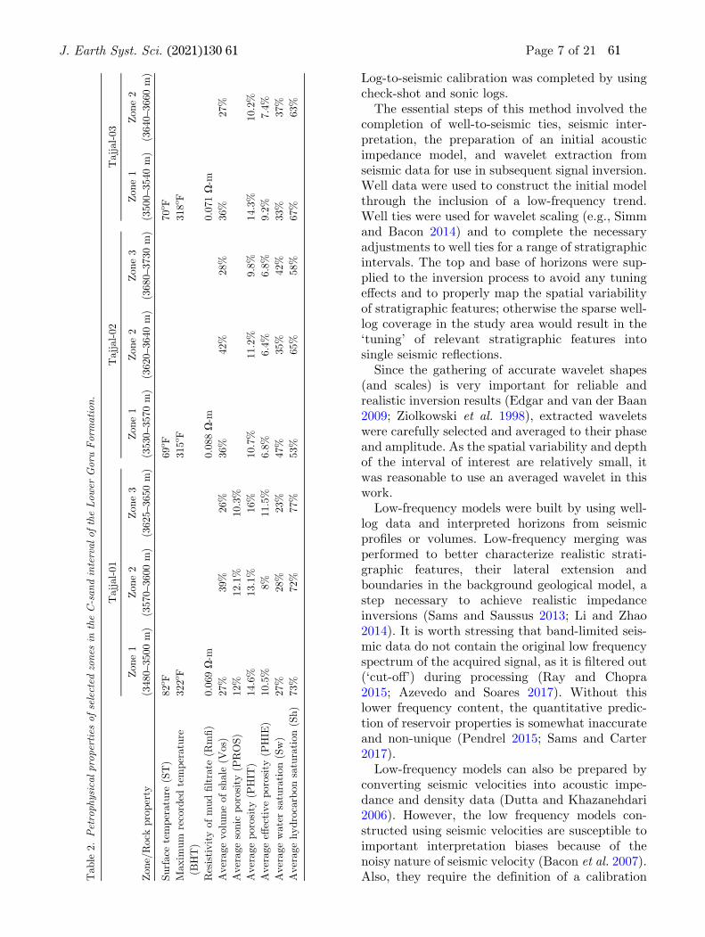
Table 2 outlines the distinct reservoir para-meters calculated with the help of petrophysicalanalyses.

3.3 Seismic inversion

Seismic inversion is the process of transformingseismic interface properties into layer properties.Hence, seismic inversion greatly helps the inter-pretation and quantiBcation of reservoir propertiesand their spatial distribution (Yilmaz 2001; Ash-croft 2011). The generalised workCow for seismicinversion applied in this study is based on Ali et al.(2018). Caveats associated with our approach arebrieCy discussed in Lindseth (1979), and Olden-burg et al. (1983, 1986).For this study we applied a model-based inver-

sion (Russell and Dommico 1988), which is a typeof deterministic inversion. Model-based inversion is

Table 1. Key recording and processing parameters of the 3D seismic dataset used in this study.

Key 3D seismic data acquisition parameters

Source Recording parameters

Vibroseis 4 Sampling interval 2 ms

No. of sweeps 4 Record length 6 s

Sweep frequency sweep length 8–80 Hz Geometry

Sweep type 16 s Receiver line interval 300 m

Sweep taper Linear Source line onterval 350 m

Receiver parameters

Number of geophones 2912

Geophone array Rectangular

Processing parameters

Vibroseis minimum phase conversion Q phase and amplitude compensation 3D prestack migration velocity analysis

Amplitude adjustment 3D surface consistent spiking deconvolution 3D full isotropic prestack time migration

Static correction Spectral Cattening (6–80 Hz) Foot print noise attenuation

3D FK coning Blter in cross

spread domain

Velocity analysis 3D FXY Random noise attenuation

Amplitude vs. oAset corrections 3D surface consistent residual static

computation and application

Filter equivalent spectral balancing

to preserve amplitude

3D surface consistent

amplitude corrections

OAset regularization DMO Time variant Blter


a broadband inversion technique that uses an ini-tial acoustic impedance model based on well-logdata together with seismic-driven velocity infor-mation and interpreted seismic horizons. Thisinitial acoustic impedance model is changed, com-pared to the original seismic data, and sequentiallyupdated until the misBt between the syntheticseismogram (obtained from convolving the waveletwith acoustic impedance), and seismic data isminimised (Veeken 2007; Ashcroft 2011; Simm andBacon 2014). Several constraints are applied torestrict the inversion solution in a geological sense.

The generalised workCow employed for model-based seismic inversion is adapted from Simm andBacon (2014).

3.4 Inversion methodology

The model-based post stack seismic inversionapplied in this study used seismic and well-logdata. A standard seismic data processing sequence,aimed at true amplitude preservation, was app-lied. The output was time-migrated, zero-phaseseismic data with a 35 Hz dominant frequency.

Figure 4. Synthetic seismogram at the location of the Tajjl-01 well, superimposed on seismic inline 1459.

Figure 5. Time-structure map of the C-sand interval of the Lower Goru Formation interpreted from 3D seismic data. The welllocations are marked on the map. Fault polygons are drawn along with contours to highlight the main structural trends in theGambat–Latif block. The colour bar shows time values in seconds.


Log-to-seismic calibration was completed by usingcheck-shot and sonic logs.The essential steps of this method involved the

completion of well-to-seismic ties, seismic inter-pretation, the preparation of an initial acousticimpedance model, and wavelet extraction fromseismic data for use in subsequent signal inversion.Well data were used to construct the initial modelthrough the inclusion of a low-frequency trend.Well ties were used for wavelet scaling (e.g., Simmand Bacon 2014) and to complete the necessaryadjustments to well ties for a range of stratigraphicintervals. The top and base of horizons were sup-plied to the inversion process to avoid any tuningeAects and to properly map the spatial variabilityof stratigraphic features; otherwise the sparse well-log coverage in the study area would result in the‘tuning’ of relevant stratigraphic features intosingle seismic reCections.Since the gathering of accurate wavelet shapes

(and scales) is very important for reliable andrealistic inversion results (Edgar and van der Baan2009; Ziolkowski et al. 1998), extracted waveletswere carefully selected and averaged to their phaseand amplitude. As the spatial variability and depthof the interval of interest are relatively small, itwas reasonable to use an averaged wavelet in thiswork.Low-frequency models were built by using well-

log data and interpreted horizons from seismicproBles or volumes. Low-frequency merging wasperformed to better characterize realistic strati-graphic features, their lateral extension andboundaries in the background geological model, astep necessary to achieve realistic impedanceinversions (Sams and Saussus 2013; Li and Zhao2014). It is worth stressing that band-limited seis-mic data do not contain the original low frequencyspectrum of the acquired signal, as it is Bltered out(‘cut-oA’) during processing (Ray and Chopra2015; Azevedo and Soares 2017). Without thislower frequency content, the quantitative predic-tion of reservoir properties is somewhat inaccurateand non-unique (Pendrel 2015; Sams and Carter2017).Low-frequency models can also be prepared by

converting seismic velocities into acoustic impe-dance and density data (Dutta and Khazanehdari2006). However, the low frequency models con-structed using seismic velocities are susceptible toimportant interpretation biases because of thenoisy nature of seismic velocity (Bacon et al. 2007).Also, they require the definition of a calibrationT

able

2.Petroph

ysical

propertiesof

selected

zones

intheC-san

dinterval

oftheLow

erGoruFormation.

Tajjal-01

Tajjal-02

Tajjal-03

Zone/Rock

property

Zone1

(3480–3500m)

Zone2

(3570–3600m)

Zone3

(3625–3650m)

Zone1

(3530–3570m)

Zone2

(3620–3640m)

Zone3

(3680–3730m)

Zone1

(3500–3540m)

Zone2

(3640–3660m)

Surface

temperature

(ST)

82oF

69oF

70oF

Maxim

um

recorded

temperature

(BHT)

322oF

315oF

318oF

ResistivityofmudBltrate

(RmB)

0.069X-m

0.088X-m

0.071X-m

Averagevolumeofshale

(Vos)

27%

39%

26%

36%

42%

28%

36%

27%

Averagesonic

porosity

(PROS)

12%

12.1%

10.3%

Averageporosity

(PHIT

)14.6%

13.1%

16%

10.7%

11.2%

9.8%

14.3%

10.2%

AverageeA

ectiveporosity

(PHIE

)10.5%

8%

11.5%

6.8%

6.4%

6.8%

9.2%

7.4%

Averagewatersaturation(Sw)

27%

28%

23%

47%

35%

42%

33%

37%

Averagehydrocarbonsaturation(Sh)

73%

72%

77%

53%

65%

58%

67%

63%


factor between wells that cross the interpretedseismic volumes or proBles (Sams and Saussus2013).Due to the unavailability of pre-stack data, it

was impossible to prepare a realistic velocity modelin this work. Hence, a broadband impedance modelwas prepared using well-log data and interpretedhorizons on the 3D seismic volume, thus helpingto interpolate any relevant information betweenwells.Seismic inversion resulted in the generation of

acoustic impedance proBle, which was further usedas an input to estimate the desired reservoirattributes, i.e., porosity. For the model-basedinversion method, a starting model constructedby interpolating well data along the interpretedseismic horizons, is changed and iterativelychecked against the seismic data. The estimatedimpedance was convolved with the extractedseismic wavelet. The comparison of modelled andseismic trace yielded the error. The inversionprocedure is stopped in case of small calculatederrors, otherwise the initial model could beupdated until the calculated error was smallenough.

3.5 Geostatistical analyses

Geostatistical techniques relate different parame-ters of interest to reservoir characterization.Reservoir parameters derived from different datasets, and of different scales, are compared to reacha meaningful geological interpretation (Kelkarand Perez 2002). The spatial distribution ofreservoir parameters is usually computed andquantiBed by geostatistical techniques (Pyrcz andDeutsch 2014). A linear relationship between well-and seismic-driven attributes, namely acousticimpedance and porosity, was established in thiswork to quantify the spatial distribution ofporosity in the entire seismic cube (Doyen 1988;Grana and Dvorkin 2011). Afterwards, estimatedporosity was calibrated at the corresponding welllocations.

4. Results

4.1 Petrophysics

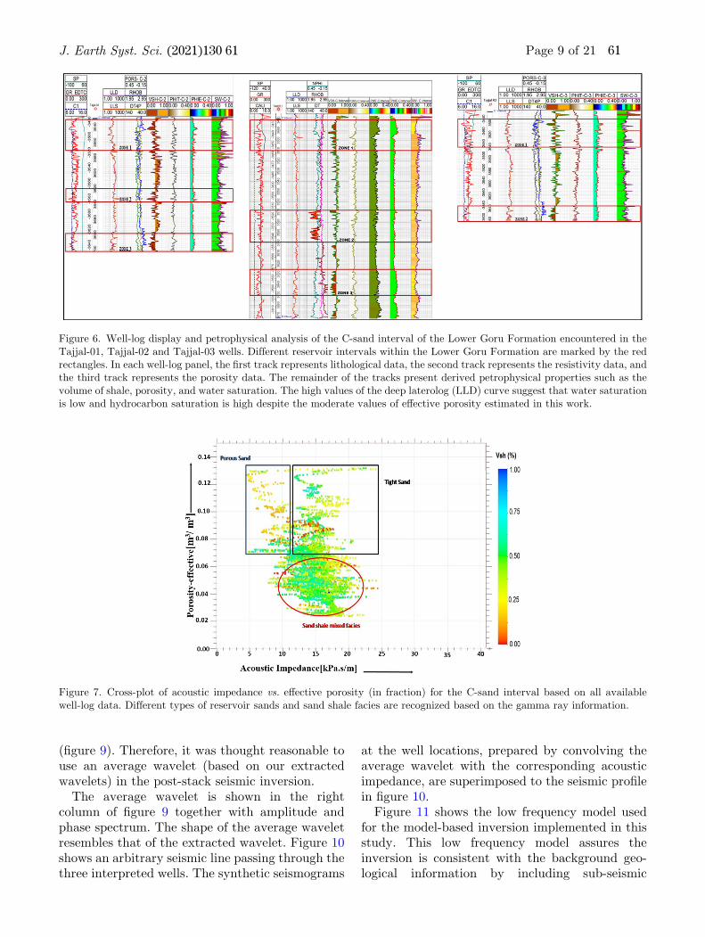
In this study, complete suites of wire-line data areused to delineate reservoir zones within the C-sand

interval of Lower Goru member (Bgure 6). Differ-ent petrophysical properties for each zone are listedin table 2. The volume of shale varies within themultiple sandy intervals of the Lower Goru For-mation. These zones exhibit variable porosity val-ues due to the presence of shale intercalations.Zone 3 is only delineated in the Tajjal-01 andTajjal-02 well. Since shale intervals within thesands can be of the laminated, structural, dispersedtypes, or any combination of these aforementionedtypes, their distribution greatly aAects the porosityof the C-sand interval (Ali et al. 2016).The cross-plot of eAective porosity, volume of

shale and acoustic impedance in Bgure 7 showsimportant details about the lithology of the C-sandinterval in all three interpreted wells. Overall, sandlayers are composed of porous (sand), tight (sand)and mixed facies (sand-shale intercalations)(Bgure 7). High eAective porosity and low impe-dance are representative of hydrocarbon-bearingporous sandstone. Sands record low eAectiveporosity with relatively high acoustic impedance,whereas low eAective porosity and an intermediaterange in acoustic impedance represent intercala-tions of sand and shale (Bgure 7).We have also applied the Lambda–Mu–Rho

(LMR) cross-plot technique to eDciently discrimi-nate between different facies (Goodway et al. 1997;Das and Chatterjee 2018). In particular, Lamb-da–Rho corresponds to the bulk impedance (in-compressibility) and Mu–Rho corresponds to theshear impedance (rigidity), and both are highlysensitive to the eAect of Cuid. In hydrocarbonsands, Lambda-Rho shows low incompressibilityvalues (Goodway et al. 1997; Das and Chatterjee2018). Figure 8 represents the result from theapplication of the LMR cross-plot technique onTajjal-01, Tajjal-02 and Tajjal-03. Gas sand, tightsand, shaly gas sand and shale facies are identiBedbased on the cut-oA values of Lambda–Rho andMu-Rho (Goodway et al. 1997; Bgure 8).

4.2 Model-based seismic inversion

The generalised workCow for our model-basedinversion is adapted from Simm and Bacon (2014).Wavelet extraction is a fundamental step in seis-mic inversion; hence, wavelets at their corre-sponding well locations were extracted from theC-sand interval of the Lower Goru Formation. Theshape and characteristic amplitude (and phase) ofwavelets do not change within the area of interest


(Bgure 9). Therefore, it was thought reasonable touse an average wavelet (based on our extractedwavelets) in the post-stack seismic inversion.The average wavelet is shown in the right

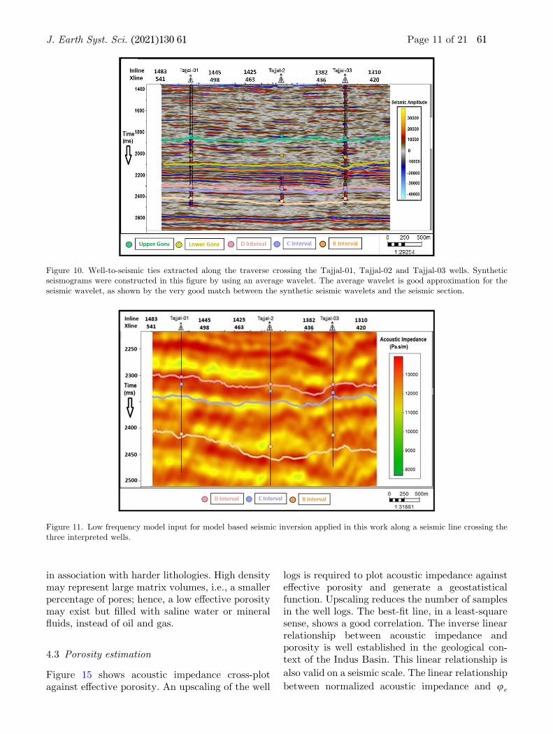
column of Bgure 9 together with amplitude andphase spectrum. The shape of the average waveletresembles that of the extracted wavelet. Figure 10shows an arbitrary seismic line passing through thethree interpreted wells. The synthetic seismograms

at the well locations, prepared by convolving theaverage wavelet with the corresponding acousticimpedance, are superimposed to the seismic proBlein Bgure 10.Figure 11 shows the low frequency model used

for the model-based inversion implemented in thisstudy. This low frequency model assures theinversion is consistent with the background geo-logical information by including sub-seismic

Figure 6. Well-log display and petrophysical analysis of the C-sand interval of the Lower Goru Formation encountered in theTajjal-01, Tajjal-02 and Tajjal-03 wells. Different reservoir intervals within the Lower Goru Formation are marked by the redrectangles. In each well-log panel, the Brst track represents lithological data, the second track represents the resistivity data, andthe third track represents the porosity data. The remainder of the tracks present derived petrophysical properties such as thevolume of shale, porosity, and water saturation. The high values of the deep laterolog (LLD) curve suggest that water saturationis low and hydrocarbon saturation is high despite the moderate values of eAective porosity estimated in this work.

Figure 7. Cross-plot of acoustic impedance vs. eAective porosity (in fraction) for the C-sand interval based on all availablewell-log data. Different types of reservoir sands and sand shale facies are recognized based on the gamma ray information.


frequencies in the Bnal computation. This stabilizesthe inversion workCow by introducing temporallimits and spatial variations to the interpretedseismic horizons (Dutta and Khazanehdari 2006;Pendrel 2015; Azevedo and Soares 2017). Due tothe non-uniqueness of seismic inversion, higher-than and lower-than-real seismic frequencies willappear in the inverted data. Therefore, it is nec-essary to use a band-pass Blter before one comparesthe inverted outputs (Veeken 2007; Li and Zhao2014).

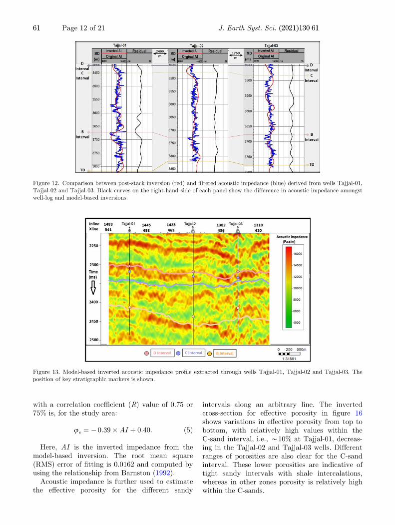
A comparison of acoustic impedance derivedfrom well- and model-based inversions is shown inBgure 12. The acoustic impedance match is goodwithin the C-sand interval; hence, the invertedacoustic impedance can be used to quantify reser-voir properties in the study area.Figure 13 shows the inverted acoustic impedance

for a cross-section joining the three explorationwells considered in this work. The upper part of theLower Goru Formation shows very high impe-dance. The B- and D-sand intervals show higheracoustic impedance when compared to the C-sandinterval (Bgure 13). The spatial variation ofacoustic impedance within the C-sand interval isalso characteristically smooth (Bgure 13).In a density section extracted along the arbitrary

line (Bgure 14), the light green and light bluecolours are representative of density values of2.5–2.6 g/cm3, typical of porous sand layers. Asand layer with high density (*2.8 g/cm3) isobserved in the upper part of the Lower GoruFormation. It is observed that density is low in theB- and C-sand intervals at Tajjal-01, while itgradually increases laterally to show relativelyhigher values in the vicinity of wells Tajjal-02 andTajjal-03. These two wells consequently show arelative decrease in porosity. Density is low in thevicinity of Tajjal-01 and increases eastwards, likely

Figure 8. Cross-plot of Lambda–rho vs. Mu–Rho for theC-sand interval utilizing all available well-log data. Differenttypes of facies are recognized based on the cut-oA values ofLambda–rho vs. Mu–Rho.

Figure 9. Wavelet extracted from the seismic data at the respective well locations. The column to the right shows the average ofcorresponding wavelets, power spectrum and phase spectrum. Despite the fact that the main lobes of wavelets appear similar,whereas their side lobes are more variable. All wavelets show similar characteristics in their corresponding power spectrum andphase spectrum plots (2nd and 3rd rows).


in association with harder lithologies. High densitymay represent large matrix volumes, i.e., a smallerpercentage of pores; hence, a low eAective porositymay exist but Blled with saline water or mineralCuids, instead of oil and gas.

4.3 Porosity estimation

Figure 15 shows acoustic impedance cross-plotagainst eAective porosity. An upscaling of the well

logs is required to plot acoustic impedance againsteAective porosity and generate a geostatisticalfunction. Upscaling reduces the number of samplesin the well logs. The best-Bt line, in a least-squaresense, shows a good correlation. The inverse linearrelationship between acoustic impedance andporosity is well established in the geological con-text of the Indus Basin. This linear relationship is

also valid on a seismic scale. The linear relationship

between normalized acoustic impedance and ue

Figure 10. Well-to-seismic ties extracted along the traverse crossing the Tajjal-01, Tajjal-02 and Tajjal-03 wells. Syntheticseismograms were constructed in this Bgure by using an average wavelet. The average wavelet is good approximation for theseismic wavelet, as shown by the very good match between the synthetic seismic wavelets and the seismic section.

Figure 11. Low frequency model input for model based seismic inversion applied in this work along a seismic line crossing thethree interpreted wells.


with a correlation coefBcient (R) value of 0.75 or75% is, for the study area:

ue ¼ � 0:39� AI þ 0:40: ð5Þ

Here, AI is the inverted impedance from themodel-based inversion. The root mean square(RMS) error of Btting is 0.0162 and computed byusing the relationship from Barnston (1992).Acoustic impedance is further used to estimate

the eAective porosity for the different sandy

intervals along an arbitrary line. The invertedcross-section for eAective porosity in Bgure 16shows variations in eAective porosity from top tobottom, with relatively high values within theC-sand interval, i.e., *10% at Tajjal-01, decreas-ing in the Tajjal-02 and Tajjal-03 wells. Differentranges of porosities are also clear for the C-sandinterval. These lower porosities are indicative oftight sandy intervals with shale intercalations,whereas in other zones porosity is relatively highwithin the C-sands.

Figure 12. Comparison between post-stack inversion (red) and Bltered acoustic impedance (blue) derived from wells Tajjal-01,Tajjal-02 and Tajjal-03. Black curves on the right-hand side of each panel show the difference in acoustic impedance amongstwell-log and model-based inversions.

Figure 13. Model-based inverted acoustic impedance proBle extracted through wells Tajjal-01, Tajjal-02 and Tajjal-03. Theposition of key stratigraphic markers is shown.


5. Discussion

Although well data provide high vertical resolutionand the best estimates for reservoir porosity, thesparse coverage of wells makes it hard to reason-ably estimate porosity in between wells. Seismicinversion helps to estimate the spatial distributionof eAective porosity in reservoir intervals con-strained by well data (Pyrcz and Deutsch 2014).The integration of petrophysics, geo-statistics,seismic surface data and seismic inversion addres-ses the problem of porosity estimation (Dolberget al. 2000; Avseth et al. 2005; Grana and Dvorkin2011; Adekanle and Enikanselu 2013; Das andChatterjee 2016).

Since well and seismic data map different aspectsof reservoir properties at different scale, theirdirect calibration might lead to unsatisfactoryresults. Uncertainties may occur if the lithofacieswithin depositional facies are not well recognizedand incorporated in subsequent stages of dataintegration. In this study, post-stack seismicinversion shows good result because absoluteacoustic impedance can capture the variations insand-shale distribution. The accuracy of the resultis judged around the well locations; away from thewell location the uncertainty will creep into theresults depending on the pattern and distributionof lithofacies. Sorting, grain distribution, reservoirconnectivity and compartmentalization may

Figure 14. Density section extracted through wells Tajjal-01, Tajjal-02 and Tajjal-03.

Figure 15. A cross-plot of normalized acoustic impedance and eAective porosity (in fraction) based on all available well-log data(Tajjal-01, Tajjal-02 and Tajjal-03) to develop a linear geostatistical relationship. The normalized acoustic impedance iscalculated by dividing each sample of acoustic impedance by the maximum of the absolute value. Such a normalized value is usedto limit dynamic range of acoustic impedance from �1 to 1.


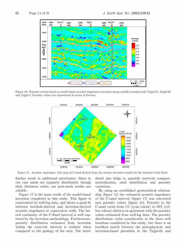
further result in additional uncertainty. Since inour case sands are regularly distributed, thoughtheir thickness varies, our post-stack results arereliable.Figure 17 is the main result of the model-based

inversion completed in this study. This Bgure isconstrained by well-log data, and shows a good Btbetween borehole-derived and inversion-derivedacoustic impedance at consecutive wells. The lat-eral continuity of the C-Sand interval is well cap-tured by the inversion methodology. Furthermore,porosity distribution estimated from inversionwithin the reservoir interval is realistic whencompared to the geology of the area. The latter

detail also helps to quantify reservoir compart-mentalization, sand distribution and porosityvariations.By using an established geostatistical relation-

ship (Bgure 15) the estimated acoustic impedanceof the C-sand interval (Bgure 17) was convertedinto porosity values (Bgure 18). Porosity in theC-sand varies from 1% (cyan colour) to 16% (yel-low colour) which is in agreement with the porosityvalues estimated from well-log data. The porositydistribution varies considerably at the three welllocations considered in this study, but there is anexcellent match between the petrophysical- andinversion-based porosities in the Tajjal-01 and

Figure 16. Porosity section based on model-based acoustic impedance inversion along a proBle crossing wells Tajjal-01, Tajjal-02and Tajjal-3. Porosity values are represented in terms of fraction.

Figure 17. Acoustic impedance (AI) map of C-sand derived from the seismic inversion results for the Gambat–Latif block.


Figure 18. Porosity distribution within the C-sand derived from the seismic inversion results for the Gambat–Latif block. Theporosity is represented in terms of fraction.

Figure 19. Cross-plot between acoustic impedance and porosity reCectivity with a linear regression Bt based on all availablewell-log data. The correlation coefBcient for this cross-plot is 84% and value of n (slope) is -0.095641.

Figure 20. Acoustic impedance and porosity wavelet. The porosity wavelet is obtained by multiplying the value of n to theacoustic impedance wavelet, and shows opposite trend to acoustic impedance wavelet.


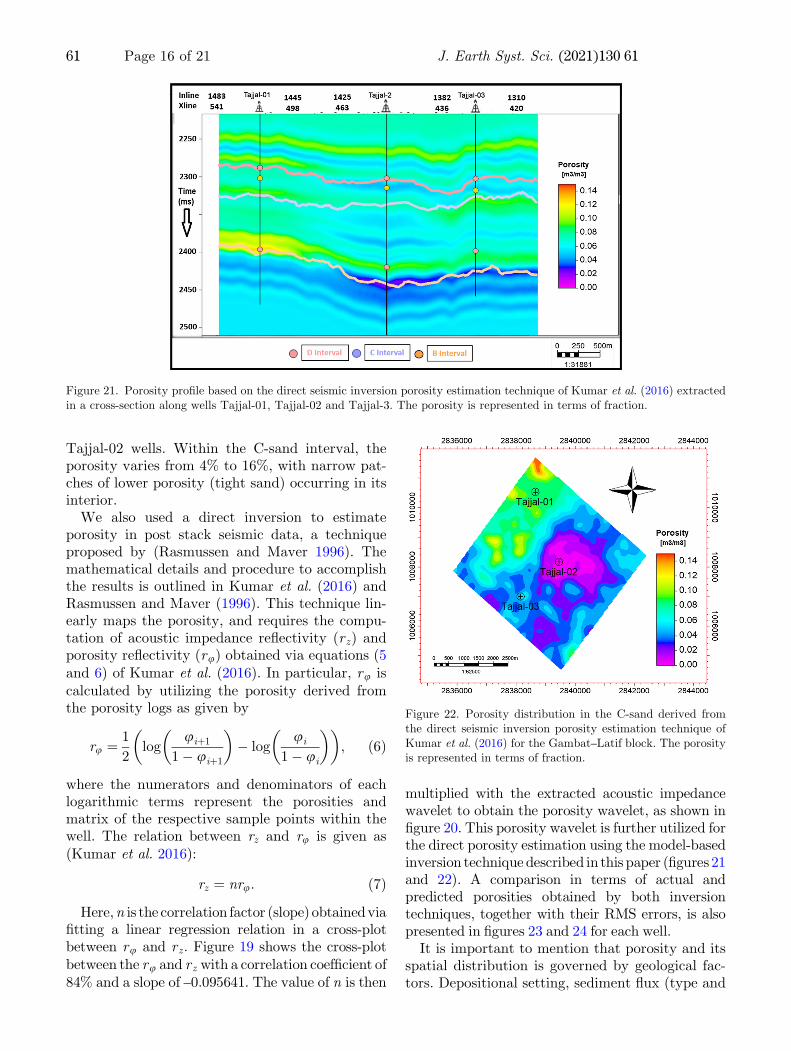
Tajjal-02 wells. Within the C-sand interval, theporosity varies from 4% to 16%, with narrow pat-ches of lower porosity (tight sand) occurring in itsinterior.We also used a direct inversion to estimate

porosity in post stack seismic data, a techniqueproposed by (Rasmussen and Maver 1996). Themathematical details and procedure to accomplishthe results is outlined in Kumar et al. (2016) andRasmussen and Maver (1996). This technique lin-early maps the porosity, and requires the compu-tation of acoustic impedance reCectivity (rz) andporosity reCectivity (ru) obtained via equations (5and 6) of Kumar et al. (2016). In particular, ru iscalculated by utilizing the porosity derived fromthe porosity logs as given by

ru ¼ 1

2log

uiþ1

1� uiþ1

� �

� logui

1� ui

� ��

; ð6Þ

where the numerators and denominators of eachlogarithmic terms represent the porosities andmatrix of the respective sample points within thewell. The relation between rz and ru is given as(Kumar et al. 2016):

rz ¼ nru: ð7Þ

Here,n is the correlation factor (slope) obtainedviaBtting a linear regression relation in a cross-plotbetween ru and rz . Figure 19 shows the cross-plotbetween the ru and rz with a correlation coefBcient of84% and a slope of –0.095641. The value of n is then

multiplied with the extracted acoustic impedancewavelet to obtain the porosity wavelet, as shown inBgure 20. This porosity wavelet is further utilized forthe direct porosity estimation using the model-basedinversion techniquedescribed in this paper (Bgures 21and 22). A comparison in terms of actual andpredicted porosities obtained by both inversiontechniques, together with their RMS errors, is alsopresented in Bgures 23 and 24 for each well.It is important to mention that porosity and its

spatial distribution is governed by geological fac-tors. Depositional setting, sediment Cux (type and

Figure 21. Porosity proBle based on the direct seismic inversion porosity estimation technique of Kumar et al. (2016) extractedin a cross-section along wells Tajjal-01, Tajjal-02 and Tajjal-3. The porosity is represented in terms of fraction.

Figure 22. Porosity distribution in the C-sand derived fromthe direct seismic inversion porosity estimation technique ofKumar et al. (2016) for the Gambat–Latif block. The porosityis represented in terms of fraction.


amount of sediment) and post depositional pro-cesses are the main factors controlling porosity. Inthe study area, there is a pronounced and appre-ciable range in porosity values due to aforemen-tioned factors. The porosity in the wells, fewkilometres apart from each other, is highly vari-able. Overall, both the inversion techniquesapplied in this study show the reasonably small

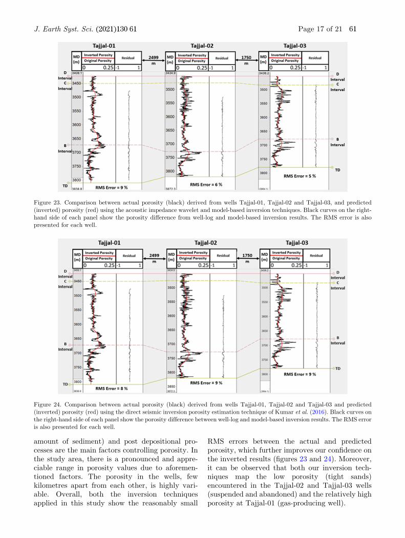
RMS errors between the actual and predictedporosity, which further improves our conBdence onthe inverted results (Bgures 23 and 24). Moreover,it can be observed that both our inversion tech-niques map the low porosity (tight sands)encountered in the Tajjal-02 and Tajjal-03 wells(suspended and abandoned) and the relatively highporosity at Tajjal-01 (gas-producing well).

Figure 23. Comparison between actual porosity (black) derived from wells Tajjal-01, Tajjal-02 and Tajjal-03, and predicted(inverted) porosity (red) using the acoustic impedance wavelet and model-based inversion techniques. Black curves on the right-hand side of each panel show the porosity difference from well-log and model-based inversion results. The RMS error is alsopresented for each well.

Figure 24. Comparison between actual porosity (black) derived from wells Tajjal-01, Tajjal-02 and Tajjal-03 and predicted(inverted) porosity (red) using the direct seismic inversion porosity estimation technique of Kumar et al. (2016). Black curves onthe right-hand side of each panel show the porosity difference between well-log and model-based inversion results. The RMS erroris also presented for each well.


It is imperative to mention that, to recognize andaddress the uncertainties related with spatialporosity mapping, multiple point simulation andstochastic inversion techniques may be applied.However, these are not within the scope of thisstudy; they require lithofacies modelling, concep-tual geological modelling, and additional data.This might result in better estimation and uncer-tainty quantiBcation but at the cost of additionalhuman and computational resources. Thus, thespatial porosity mapping in this study may be usedas an input for further sophisticated modelling.

6. Conclusions

Spatial porosity estimation and mapping is a chal-lenging task, especially in the casewhere limited dataof different scales is available. In this work, spatialporosity is estimated and mapped in the Gam-bat–Latif block in the Central Indus Basin, Pakistanby using model based post-stack seismic inversion.The estimated porosity values range from 1 to 16% inthe studied reservoir zone. Variations in the spatialdistribution of porosity within the C-sand interval ofthe Lower Goru Formation are due to the presence ofshale, and to the style(s) of shale distribution withinsand intervals. These uncertainties associated withspatial porosity mapping are difBcult to capture andquantify due to resolvingpower of seismic, datasets ofdifferent scales and the geostatistical relationshipsthat are valid in the vicinity of wells. The initial lowfrequency model, constructed from seismic and welldata interpretation, is a crucial parameter for theinversion workCow. It may be concluded that poros-ity mapping by post-stack seismic inversion wasdeemed reliable in this study, andmaybe so in similarscenarios. It is hoped that this case study willencourage further studies touseother techniques, i.e.,multipoint Geostatistical simulations and stochasticinversions to Bnd a more realistic geological consis-tent models for porosity distributions. However, thelatter methods demand more data, their scaling, andfurther human and computational resources.

Acknowledgements

The authors would like to thank DirectorateGeneral of Petroleum Concessions (DGPC), Pak-istan, for allowing the use of seismic and well-logdata for research and publication purposes andDepartment of Earth Sciences, Quaid-i-Azam

University, Islamabad, Pakistan, CardiA Univer-sity, UK for providing the basic requirements tocomplete this work. We are thankful to thereviewers/Associate Editor of this manuscript forcritically reviewing and improving the manuscript.

Author statement

Dr Muhammad Toqeer perceived the idea andpartially executed this idea of the research. DrAamir Ali took the idea and proposed themethodology and implemented it with the help ofhis student Mr Ashar Khan. Mr Ashar Khan hascontribution in terms of collection of the literatureand raw data. Dr Tiago M Alves have given thesupport in terms of modern research methods andhelped in the interpretation of the data. Mr Zubairhas given the software and data support andcomputed the maps. Dr Matloob Hussain hascontributed in interpretation and Bnalization of themanuscript.

References

Abbasi S, Kalwar Z and Solangi S 2016 Study of structuralstyles and hydrocarbon potential of Rajan Pur Area,Middle Indus Basin, Pakistan; BUJ ES 1 36–41.

Afzal J, Williams M and Aldridge R 2009 Revised stratigraphyof the lower Cenozoic succession of the Greater Indus Basinin Pakistan; J. Micropalaeontol. 28 7–23.

Ahmed N, Fink P, Sturrock S, Mahmoo T and Ibrahim M 2004Sequence stratigraphy as predictive tool in Lower GoruFairway, Lower And Middle Indus Platform, Pakistan,Pakistan Association of Petroleum Geoscientists, AnnualTechnical Conference, Islamabad, pp. 17–18.

Akhter G, Ahmed Z, Ishaq A and Ali A 2015 Integratedinterpretation with Gassmann Cuid substitution for opti-mum Beld development of Sanghar area, Pakistan: A casestudy; Arab. J. Geosci. 8 7467–7479.

Adekanle A and Enikanselu P A 2013 Porosity prediction fromseismic inversion properties over ‘XLD’Field, Niger Delta;Am. J. Sci. Indus. Res. 4(1) 31–35.

Alavi M 2004 Regional stratigraphy of the Zagros fold–thrustbelt of Iran and its proforeland evolution; Am. J. Sci. 3041–20, https://doi.org/10.2475/ajs.304.1.1.

Ali A, Alves T M, Saad F A, Ullah M, Toqeer M and HussainM 2018 Resource potential of gas reservoirs in SouthPakistan and adjacent Indian subcontinent revealed bypost-stack inversion techniques; J. Nat. Gas Sci. Eng. 4941–55.

Ali A, Hussain M, Rehman K and Toqeer M 2016 EAect ofshale distribution on hydrocarbon sands integrated withanisotropic rock physics for AVA modelling: A case study;Acta Geophys. 64 1139–1163.

Angeleri G P and Carpi R 1982 Porosity prediction fromseismic data; Geophys. Prospect 30 580–607, https://doi.org/10.1111/j.1365-2478.1982.tb01328.x.


Anwer H M, Ali Alves T M and Zubair A 2017 EAects of sand-shale anisotropy on amplitude variation with angle (AVA)modelling: The Sawan gas Beld (Pakistan) as a key casestudy for South Asia’s sedimentary basins; J. Asian EarthSci. 147 516–531, https://doi.org/10.1016/j.jseaes.2017.07.047.

Ashcroft W 2011 A Petroleum Geologist’s Guide to SeismicReCection, Wiley–Blackwell.

Avseth P, Mukerji T and Mavko G 2005 Quantitative seismicinterpretation: Applying rock physics tools to reduce inter-pretation risk, Cambridge University Press, https://doi.org/10.1017/CBO9780511600074.

Azeem T, Chun W, Khalid P and Qing L 2017 An integratedpetrophysical and rock physics analysis to improve reser-voir characterization of Cretaceous sand intervals in MiddleIndus Basin, Pakistan; J. Geophys. Eng. 14 212–225.

Azevedo L, Amaro C, Grana D, Soares A and Guerreiro L 2017Coupling geostatistics and rock physics in reservoir mod-elling and characterization; Soc. Petrol. Eng., https://doi.org/10.2118/188470-MS.

Azevedo L and Soares A 2017 Geostatistical methods forreservoir geophysics: Advances in oil and gas exploration &production, Springer, Cham, https://doi.org/10.1007/978-3-319-53201-1.

Aziz O, Hussain T, Ullah M, Bhatti A S and Ali A 2018Seismic based characterization of total organic content fromthe marine Sembar shale, Lower Indus Basin, Pakistan;Mar. Geophys. Res; 39(4) 491–508.

Bacon M, Simm R and Redshaw T 2007 3-D seismicinterpretation, Cambridge University Press, https://doi.org/10.1017/CBO9780511802416.

Barnston A G 1992 Correspondence among the correlation,RMSE, and Heidke forecast veriBcation measures: ReBne-ment of the Heidke score; Wea. Forecast. 7(4) 699–709.

Berger A, Gier S and Krois P 2009 Porosity-preservingchlorite cements in shallow–marine volcaniclastic sand-stones: Evidence from Cretaceous sandstones of the Sawangas Beld, Pakistan; AAPG Bull. 93 595–615.

Bosch M, Carvajal C, Rodrigues J, Torres A, Aldana M andSierra J 2009 Petrophysical seismic inversion conditioned towell-log data: Methods and application to a gas reservoir;Geophysics 74 O1–O15, https://doi.org/10.1190/1.3043796.

Bosch M, Mukerji T and Gonzalez E F 2010 Seismic inversionfor reservoir properties combining statistical rock physicsand geostatistics: A review; Geophysics 75 75A165,https://doi.org/10.1190/1.3478209.

Caers J, Avseth P and Mukerji T 2001 Geostatisticalintegration of rock physics, seismic amplitudes, and geo-logic models in North Sea turbidite systems; Lead Edge 20308, https://doi.org/10.1190/1.1438936.

Chen Q and Sidney S 1997 Seismic attribute technology forreservoir forecasting and monitoring; Lead Edge 16445–448, https://doi.org/10.1190/1.1437657.

Chopra S and Marfurt K J 2007 Seismic attributes for prospectidentiBcation and reservoir characterization; Geophys. Dev.Ser. 11 465, https://doi.org/10.1190/1.9781560801900.

Das B and Chatterjee R 2016 Porosity mapping from inversionof post–stack seismic data; Georesursy 18(4) 306–313.

Das B and Chatterjee R 2018 Well log data analysis forlithology and Cuid identiBcation in Krishna–GodavariBasin, India; Arab. J. Geosci. 11(10) 231.

Das B, Chatterjee R, Singha D K and Kumar R 2017 Post-stack seismic inversion and attribute analysis in shallowoAshore of Krishna-Godavari basin, India; J. Geol. Soc.India 90 32–40, https://doi.org/10.1007/s12594-017-0661-4.

de Terra H, de Chardin P T and Paterson T T 1936 Jointgeological and prehistoric studies of the late Cenozoic inIndia; Science 83 233–236.

Delaplanche J, Lafet Y and Sineriz B 1982 Seismic reCectionapplied to sedimentology and gas discovery in the Gulf ofCadiz; Geophys. Prospect. 30 1–24.

Dolberg D, Helgesen J, Hanssen T, Magnus I, Saigal G andPedersen B 2000 Porosity prediction from seismic inversion,Lavrans Field, Halten Terrace, Norway; Lead Edge 19392–399, https://doi.org/10.1190/1.1438618.

Doyen P 1988 Porosity from seismic data: A geostatisticalapproach; Geophysics 53 1263–1275, https://doi.org/10.1190/1.1442404.

Dutta N and Khazanehdari J 2006 Estimation of formationCuid pressure using high-resolution velocity from inversionof seismic data and a rock physics model based oncompaction and burial diagenesis of shales; Lead Edge 251528–1539, https://doi.org/10.1190/1.2405339.

Edgar J and van der Baan M 2009 How reliable is statisticalwavelet estimation. In: SEG Technical Program ExpandedAbstracts 2009, Society of Exploration Geophysicists,pp. 3233–3237, https://doi.org/10.1190/1.3255530.

Gogoi T and Chatterjee R 2019 Estimation of petrophysicalparameters using seismic inversion and neural networkmodelling in Upper Assam basin, India; Geosci. Frontiers10(3) 1113–1124, https://doi.org/10.1016/j.gsf.2018.07.002.

Goodway B, Chen T and Downtown J 1997 Improved AVOCuid detection and lithology discrimination using Lamepetrophysical parameters, 67th Annual international Meet-ing, SEG Expanded Abstracts, pp. 183–186.

Grana D and Dvorkin J 2011 The link between seismicinversion, rock physics, and geostatistical simulations inseismic reservoir characterization studies; Lead Edge 3054–61, https://doi.org/10.1190/1.3535433.

Hearts J R, Nelson P H and Paillet F L 2002 Well Logging forPhysical Properties: A Handbook for Geophysicists, Geol-ogists and Engineers, 2nd edn, John Wiley & Sons,Chichester.

Iravani M, Rastegarnia M, Javani D, Sanati A and Hajiabadi SH 2017 Application of seismic attribute technique toestimate the 3D model of hydraulic Cow units: A casestudy of a gas Beld in Iran; Egypt. J. Pet., https://doi.org/10.1016/j.ejpe.2017.02.003.

Jafari M, Nikrouz R and Kadkhodaie A 2017 Estimation ofacoustic-impedance model by using model-based seismicinversion on the Ghar Member of Asmari Formation in anoil Beld in southwestern Iran; Lead Edge 36 487–492.

Kadri I 1995 Petroleum geology of Pakistan, PakistanPetroleum Limited, Karachi.

Karbalaali H, Shadizadeh S and Riahi M 2013 Delineatinghydrocarbon bearing zones using elastic impedance inver-sion: A Persian Gulf example; Iran. J. Oil. Gas. Sci. Tech. 28–19.

Kazmi A and Abbasi I 2008 Stratigraphy & Historical Geologyof Pakistan, Department & National Centre of Excellence inGeology, Peshwar, Pakistan.


Kazmi A H and Rana R A 1982 Tectonic map of Pakistan1:2000000: Map showing structural features and tectonicstages in Pakistan, Geological survey of Pakistan.

Kelkar M and Perez G 2002 Applied Geostatistics forReservoir Characterization, Society of PetroleumEngineers.

Khattak F, Shafeeq M and Mansoor A 1999 Regional trends inporosity and permeability of reservoir horizons of LowerGoru Formation, Lower Indus Basin, Pakistan; J. Hydro-carb. Res. 11 37–50.

King D E 1990 Incorporating geological data in well loginterpretation; In: Geological Applications of WirelineLogs, pp. 45–55, https://doi.org/10.1144/gsl.sp.1990.048.01.06.

Kumar R, Das B, Chatterjee R and Sain K 2016 A method-ology of porosity estimation from inversion of post-stackseismic data; J. Nat. Gas Sci. 28 356–364.

Landa J L, Horne R N, Kamal M M and Jenkins C D 2000reservoir characterization constrained to well-test data: ABeld example; SPE Reserv. Eval. Eng. 3 325–334, https://doi.org/10.2118/65429-PA.

Leite E P and Vidal A C 2011 3D porosity prediction fromseismic inversion and neural networks; Comput. Geosci. 371174–1180, https://doi.org/10.1016/j.cageo.2010.08.001.

Li M and Zhao Y 2014 Chapter 6 – Seismic inversiontechniques. In: Geophysical Exploration Technology Appli-cations in Lithological and Stratigraphic Reservoirs, Else-vier, Oxford, pp. 133–198, https://doi.org/10.1016/B978-0-12-410436-5.00006-X.

Lindseth R O 1979 Synthetic sonic logs – a process forstratigraphic interpretation; Geophysics 44 3, https://doi.org/10.1190/1.1440922.

Liner C 2016 Elements of 3D seismology, investigations ingeophysics; Society of Exploration Geophysicists, https://doi.org/10.1190/1.9781560803386.

Mukerji T, Avseth P, Mavko G, Takahashi I and Gonz�alez E F2001 Statistical rock physics: Combining rock physics,information theory, and geostatistics to reduce uncertaintyin seismic reservoir characterization; Lead Edge 20 313,https://doi.org/10.1190/1.1438938.

Oldenburg D, Levy S and Stinson K 1986 Inversion of band-limited reCection seismograms: Theory and practice; Proc.IEEE 74 487–497.

Oldenburg D, Scheuer T and Levy S 1983 Recovery of theacoustic impedance from reCection seismograms; Geo-physics 48 1318–1337.

Pendrel J 2015 Low frequency models for seismic inversions:Strategies for success. In: SEG Technical ProgramExpanded Abstracts 2015, Society Exploration Geophysi-cists, pp. 2703–2707, https://doi.org/10.1190/segam2015-5843272.1.

Pyrcz M and Deutsch C V 2014 Geostatistical ReservoirModelling, 2nd edn, Oxford University Press.

Quadri S V 1986 Hydrocarbon prospects of southern Indusbasin, Pakistan; Am. Assoc. Pet. Geol. Bull. 70 730–747.

Rasmussen K B and Maver K G 1996 Direct inversion forporosity of post stack seismic data. NPF/SPE European3-D Reservoir Modelling Conference, pp. 235–246, https://doi.org/10.2523/35509-ms.

Ray A and Chopra S 2015 More robust methods of low-frequency model building for seismic impedance inversion.In: SEG Technical Program Expanded Abstracts 2015,

Society of Exploration Geophysicists, pp. 3398–3402,https://doi.org/10.1190/segam2015-5851713.1.

Robison C R, Smith M A and Royle R A 1999 Organic facies inCretaceous and Jurassic hydrocarbon source rocks, South-ern Indus basin, Pakistan; Int. J. Coal Geol. 39 205–225,https://doi.org/10.1016/S0166-5162(98)00046-9.

Rosa A L R 2018 The seismic signal and its meaning; In: Theseismic signal and its meaning, Society of ExplorationGeophysicists, https://doi.org/10.1190/1.9781560803348.

Russell B and Dommico S 1988 Introduction to seismicinversion methods, SEG.

Sams M and Carter D 2017 Stuck between a rock and areCection: A tutorial on low-frequency models for seismicinversion; Interpretation 5 B17–B27.

Sams M and Saussus D 2013 Practical implications of lowfrequency model selection on quantitative interpretationresults; SEG Tech. Progr. Expand. Abstr., pp. 3118–3122.

Silva M Da, Rauch-Davies M and Cuervo A 2004 Dataconditioning for a combined inversion and AVO reservoircharacterisation study, 66th EAGE Conf.

Simm R and Bacon M 2014 Seismic Amplitude: An inter-preter’s handbook, Cambridge University Press.

Singha D K, Shukla P K, Chatterjee R and Sain K 2019 Multi-channel 2D seismic constraints on pore pressure- andvertical stress-related gas hydrate in the deep oAshore ofthe Mahanadi Basin, India; J. Asian Earth Sci., https://doi.org/10.1016/j.jseaes.2019.103882.

Sinha B and Mohanty P 2015 Post stack inversion for reservoircharacterization of KG Basin associated with gas hydrateprospects; J. Ind. Geophys. Union 19 200–204.

Teixeira L and Maul A 2020 Quantitative and stratigraphicseismic interpretation of the evaporite sequence in thesantos basin, Elsevier, https://www.sciencedirect.com/science/article/abs/pii/S0264817220304736.

Tiab D and Donaldson E 2015 Petrophysics: Theory andPractice of Measuring Reservoir Rock and Cuid TransportProperties, Gulf Professional Publishing.

Toqeer M and Ali A 2017 Rock physics modelling in reservoirswithin the context of time lapse seismic using well log data;Geosci. J. 21 111–122.

Veeken P C H 2007 Seismic Stratigraphy, Basin Analysis andReservoir Characterisation, Elsevier, Amsterdam.

Veeken P C H and Rauch-Davies M 2006 AVO attributeanalysis and seismic reservoir characterization; First Break24 41–52, https://doi.org/10.3997/1365-2397.2006004.

Veeken P C H and Da Silva M 2004 Seismic inversion methodsand some of their constraints; First Break 22 47–70.

Verma S, Bhattacharya S, Lujan B, Agrawal D and Mallick S2018 Delineation of early Jurassic aged sand dunes andpaleo-wind direction in southwestern Wyoming using seis-mic attributes, inversion, and petrophysical modelling; J.Nat. Gas Sci. Eng. 60 1–10, https://doi.org/10.1016/j.jngse.2018.09.022.

Walls J, Dvorkin J and Carr M 2004 Well logs and rockphysics in seismic reservoir characterization; OAshoreTechnol. Conf., https://doi.org/10.4043/16921-MS.

Wandrey C, Law B and Shah H 2004 Sembar Goru/Ghazijcomposite total petroleum system, Indus and Sulai-man–Kirthar geologic provinces, Pakistan and India; In:Petroleum Systems and Related Geologic Studies in Region8, South Asia (ed.) Wandrey C J, United States GeologicalSurvey Bulletin, 2208-C.


Wang Y 2017 Seismic Inversion: Theory and Applications,Wiley Blackwell.

White R 2003 Tying well-log synthetic seismograms to seismicdata: The key factors; In: SEG Technical ProgramExpanded Abstracts 2003, Society Exploration Geophysi-cists, pp. 2449–2452, https://doi.org/10.1190/1.1817885.

Williams M D 1959 Stratigraphy of the Lower Indus Basin,West Pakistan; In: 5th, New York. Proc, World PetroleumCongress, pp. 377–394.

Yao F and Gan L 2000 Application and restriction of seismicinversion; Pet. Explor. Dev. 27 53–56.

Yilmaz €O 2001 Seismic data analysis: Processing, inversion,and interpretation of seismic data, investigations in

geophysics; Society of Exploration Geophysicists, https://doi.org/10.1190/1.9781560801580.

Zaigham N and Mallick K 2000 Prospect of hydrocarbonassociated with fossil-rift structures of the southernIndus basin, Pakistan; AAPG Bull. 84 1833–1848.

Zhang R, Sen M K, Phan S and Srinivasan S 2012 Stochasticand deterministic seismic inversion methods for thin-bedresolution; J. Geophys. Eng. 9(5) 611–618, https://doi.org/10.1088/1742-2132/9/5/611.

Ziolkowski A M, Underhill J R and Johnston R G K 1998Wavelets, well-ties, and the search for stratigraphic traps;Geophysics 63 297–313.

Corresponding editor: ARKOPROVO BISWAS


Documents

Application of model based post-stack inversion in the