QUEST

APPLICATION OF QUANTITATIVE RISKANALYSIS TO CODE-REQUIRED SITING

STUDIES INVOLVING HAZARDOUS MATERIALTRANSPORTATION ROUTES

John B. Cornwell and Jeffrey D. Marx

Presented AtCenter for Chemical Process Safety

17th Annual International Conference and WorkshopRisk, Reliability, and Security

Jacksonville, FloridaOctober 8-11, 2002

Presented ByQuest Consultants Inc.®

908 26th Avenue N.W.Norman, Oklahoma 73069Telephone: 405-329-7475

Fax: 405-329-7734E-mail: info@questconsult.com

URL: http://www.questconsult.com/

Copyright© 2002, Quest Consultants Inc., 908 26th Avenue N.W., Norman, Oklahoma 73069, USA. All rights reserved.Copyright is owned by Quest Consultants Inc. Any person is hereby authorized to view, copy, print, and distribute documents subject to the followingconditions.

1. Document may be used for informational purposes only.2. Document may only be used for non-commercial purposes.3. Any document copy or portion thereof must include this copyright notice.

QUEST-1-

APPLICATION OF QUANTITATIVE RISK ANALYSIS TOCODE-REQUIRED SITING STUDIES INVOLVING

HAZARDOUS MATERIAL TRANSPORTATION ROUTES

John B. Cornwell and Jeffrey D. MarxQuest Consultants Inc.908 26th Avenue N.W.

Norman, Oklahoma 73069jbc@questconsult.com

ABSTRACT

Although the United States Federal Government does not have a risk-based standard fordetermining the acceptability of a location relative to the transportation of hazardousmaterials, a number of state and local regulatory agencies are beginning to require that a riskanalysis be performed as part of a siting study. An example of such a legal requirement isthe California Code of Regulations, Title 5, Section 14010. This regulation explicitlyrequires that a risk analysis be performed on hazardous material pipelines and rail cargotransportation routes within 1,500 feet of a proposed public school site.

With only a handful of companies able to perform true Quantitative Risk Analysis (QRA)studies (not qualitative assessments), a method was needed that could apply the results of aseries of QRA studies to any proposed location. This can be achieved by developing risktransects for a range of hazardous material pipelines and railcar cargoes. Risk transectscreate a relationship between individual risk and distance from the pipeline or railway. Byvarying the commodity, line diameter, and operating pressure for the pipelines, and tankcapacity and commodity for the railcars, a set of risk transects can be created that can thenbe applied to any proposed location. This paper outlines the process of developing theconsequence modeling, accident probability data, and risk calculations that are necessary tocreate risk transects. It also demonstrates how the risk transects can be combined and usedto satisfy the risk analysis requirements contained in the California regulations.

INTRODUCTION

Building a new school in California now requires a risk analysis for the proposed site, subject to CaliforniaCode of Regulations, Title 5, Division 1, Chapter 13, Subchapter 1, School Facilities Construction, Section14010. Specifically, Subparts (d) and (h) outline the type of analysis to be performed.

(d) If the proposed site is within 1,500 feet of a railroad track easement, a safety studyshall be done by a competent professional trained in assessing cargo manifests,frequency, speed, and schedule of railroad traffic, grade, curves, type and condition

QUEST-2-

of track, need for sound or safety barriers, need for pedestrian and vehicle safe-guards at railroad crossings, presence of high pressure gas lines near the tracks thatcould rupture in the event of a derailment, preparation of an evacuation plan. Inaddition to the analysis, possible and reasonable mitigation measures must be iden-tified.

(h) The site shall not be located near an aboveground water or fuel storage tank, or with-in 1,500 feet of the easement of an aboveground or underground pipeline that canpose a safety hazard, as determined by a risk analysis study, conducted by a compe-tent professional, which may include certification from a local public utility com-mission.

Because of the difficult nature of performing a true Quantitative Risk Analysis (QRA) study, a simplifiedmethod for applying hazardous material transportation QRA results to any proposed location was needed.By creating generic risk transects for varying pipeline and railcar commodities (with their appropriate proper-ties), the risk at any particular location could be found. Generic risk transects provide a “worst-case” estimateof the risk in the vicinity of a pipeline or railway. Once these are generated, they can be applied to any siteas a check for acceptability, since risk transects are a simple relationship between individual risk and distancefrom the pipeline or railway.

To demonstrate the methodology behind creating this set of risk transects, the hazards for an example set ofpipelines and railcars were modeled with the proper consequence modeling, and accident frequencies weredeveloped for potential release with applicable data. These were combined to create a risk transect for eachof the following pipelines and railcar systems.

Pipelines30-inch natural gas pipeline operating at 1,000 psig12-inch natural gas pipeline operating at 700 psig8-inch LPG pipeline operating at 450 psig6-inch anhydrous ammonia pipeline operating at 330 psig

RailcarsLPG railcar, 33,000 gallonsChlorine railcar, 90 tonsAnhydrous ammonia railcar, 33,000 gallons

CONSEQUENCE MODELING

From the public’s perception, it is safe to assume that the consequence modeling of potential hazards associat-ed with pipeline and railcar transport of flammable and toxic materials is perceived as more important thanthe associated statistical analysis of how often a release may occur. After all, if the consequence modelingshows that a release will not impact a proposed school location, then there is no need to continue the riskstudy. To some degree, the regulations have already limited the range of study by excluding from review anypipeline or railway that is more than 1,500 feet from the proposed school location. However, the effects ofmany hazardous materials transported by pipeline and railcar, such as liquefied petroleum gas (LPG),anhydrous ammonia, chlorine, etc., can easily reach 1,500 feet or more under a wide range of release andatmospheric conditions. The reasoning behind this limitation in the regulations is not defined and may simplycome from “experience.”

QUEST-3-

Experience will tell the modeling analyst that a release of gas or liquefied gas from any hole size (leak,puncture, or rupture in a pipeline) will result in the formation of a free jet. Jet releases will exhibit rapid mix-ing of the released material with the surrounding air due to the turbulence generated by the high velocity ofthe gas (or gas/aerosol mixture) as it enters the surrounding air.

A pressurized release of gas or liquid from a buried pipeline often displaces the overburden (soil), resultingin a free flowing jet of gas entering the atmosphere. Overburden displacement is characterized by the forma-tion of a “crater” around the rupture. Creation of a crater (overburden removal) is dependent on the available“force” that the fluid has upon release. Large releases of medium to high pressure gas or liquid are usuallycapable of creating a crater. The crater allows the fluid to enter the atmosphere with high velocity and actas a free jet.

A review of several gas pipeline accidents investigated by the United States National Transportation SafetyBoard (NTSB) indicates that, for gas pipelines with operating pressures above 600 psig, a 1-inch diameterhole will blow away the overburden above the pipeline, resulting in the formation of a crater that allows thegas to escape as an unobstructed free jet. For the purposes of this analysis, the assumption was made that rup-tures and punctures (1-inch holes) of the anhydrous ammonia, LPG, and high pressure natural gas pipelineswere capable of crater formation, resulting in a free jet release.

A leak or puncture in an anhydrous ammonia, LPG, or chlorine railcar will release the liquefied gas in muchthe same manner as a release from the pipeline. The primary difference will be that the railcar is aboveground; thus, it is not necessary to form a crater and the liquid inventory in the railcar will serve to maintainthe flow out of the hole until the liquid level drops below the elevation of the hole.

When performing site-specific consequence analysis studies, the ability to accurately model the release, dilu-tion, and dispersion of gases and aerosols is important if an accurate assessment of potential exposure is tobe attained. For this reason, Quest uses a modeling package, CANARY by Quest7, that contains a set ofcomplex models that calculate release conditions, initial dilution of the vapor (dependent upon releasecharacteristics), and the subsequent dispersion of the vapor introduced into the atmosphere. The models con-tain algorithms that account for thermodynamics, mixture behavior, transient release rates, gas cloud densityrelative to air, initial velocity of the released gas, and heat transfer effects from the surrounding atmosphereand the substrate. The release and dispersion models contained in the QuestFOCUS package (the predecessorto CANARY by Quest) were reviewed in a United States Environmental Protection Agency (EPA) sponsoredstudy [TRC, 1991] and an American Petroleum Institute (API) study [Hanna, Strimaitis, and Chang, 1991].In both studies, the QuestFOCUS software was evaluated on technical merit (appropriateness of models forspecific applications) and on model predictions for specific releases. One conclusion drawn by both studieswas that the dispersion software tended to overpredict the extent of the gas cloud travel, thus resulting in toolarge a cloud when compared to the test data (i.e., a conservative approach).

A study prepared for the Minerals Management Service [Chang, et al.,1998] reviewed models for use inmodeling routine and accidental releases of flammable and toxic gases. CANARY by Quest received thehighest possible ranking in the science and credibility areas. In addition, the report recommends CANARYby Quest for use when evaluating toxic and flammable gas releases. The specific models (e.g., SLAB) con-tained in the CANARY by Quest software package have also been extensively reviewed.

Introduction to Physiological Effects of Fires, Explosions, and Toxic Gas Exposure

The QRAs performed on the pipeline and railway routes involved the evaluation of thousands of potentialhazardous material releases. Each potential release may result in one or more of the following hazards.

QUEST-4-

(1) Exposure to gas containing a toxic component (e.g., NH3, Cl2).(2) Exposure to heat radiation from torch fires (gas released from aboveground pipeline locations, or

releases that result from excavation accidents, or releases that result from pipeline ruptures or punc-tures in which the overburden is blown away and a crater is formed, or a release from a railcar).

(3) Exposure to explosion overpressure following the release and ignition of liquefied gas (e.g., LPG).(4) Exposure to a flash fire following the release and ignition of pipeline gas or liquefied gas.(5) Exposure to heat radiation from a Boiling Liquid Expanding Vapor Explosion (BLEVE) of an LPG

railcar.

In order to compare the risks associated with each type of hazard listed above, a common measure of conse-quence must be defined. In risk analysis studies, a common measure for such hazards is their impact onhumans. For each of the fire, explosion, and toxic hazards listed, there are data available that define the effectof the hazard on humans.

When comparing a flammable hazard to an overpressure hazard, the magnitude of the hazard’s impact onhumans must be identically defined. For instance, it would not be meaningful to compare human exposureto nonlethal overpressures (e.g., low overpressures that break windows) to human exposure to thermal radi-ation causing second-degree skin burns (e.g., 37.5 kW/m2 for thirty seconds) or to lethal exposure to ammoniavapor (e.g., 3,135 ppm for fifteen minutes)

In this study, risk is defined as the potential exposure of humans to lethal hazards (i.e., radiant heat, over-pressure, or toxic gas exposure) that have the potential to occur as a result of accidents originating along thepipeline and railway routes. Lethal exposure levels for the various hazards are discussed in the followingsections.

Physiological Effects of Exposure to Thermal Radiation from Fires

The physiological effect of fire on humans depends on the rate at which heat is transferred from the fire tothe person, and the time the person is exposed to the fire. Even short-term exposure to high heat flux levelsmay be fatal. This situation could occur when persons wearing ordinary clothes are inside a flammable vaporcloud (defined by the lower flammable limit) when it is ignited. Persons located outside a flammable cloudwhen it is ignited will be exposed to much lower heat flux levels. If the person is far enough from the edgeof the flammable cloud, the heat flux will be incapable of causing fatal injuries, regardless of exposure time.Persons closer to the cloud, but not within it, will be able to take action to protect themselves (e.g., movingfarther away as the flames approach, or seeking shelter inside structures or behind solid objects).

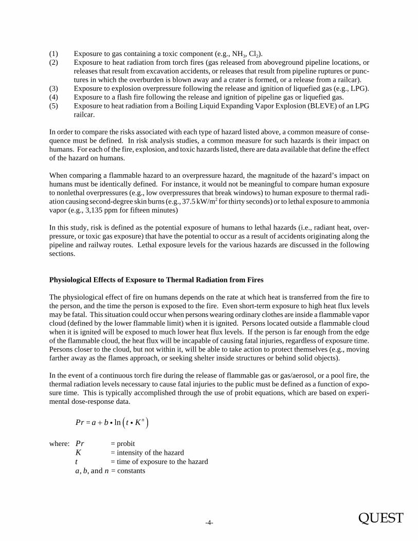
In the event of a continuous torch fire during the release of flammable gas or gas/aerosol, or a pool fire, thethermal radiation levels necessary to cause fatal injuries to the public must be defined as a function of expo-sure time. This is typically accomplished through the use of probit equations, which are based on experi-mental dose-response data.

=Pr ( )ln na b t K+ i i

where: = probitPr= intensity of the hazardK= time of exposure to the hazardt= constants, , anda b n

QUEST-5-

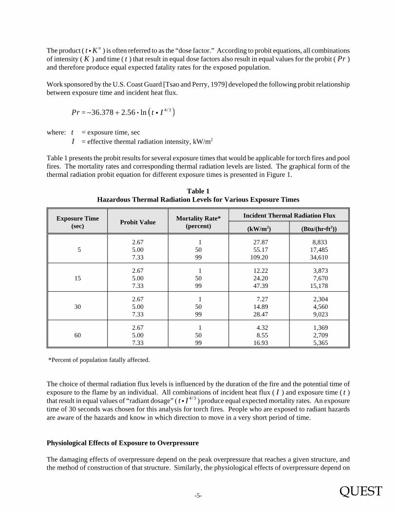
The product ( ) is often referred to as the “dose factor.” According to probit equations, all combinationsnt Kiof intensity ( ) and time ( ) that result in equal dose factors also result in equal values for the probit ( )K t Prand therefore produce equal expected fatality rates for the exposed population.

Work sponsored by the U.S. Coast Guard [Tsao and Perry, 1979] developed the following probit relationshipbetween exposure time and incident heat flux.

=Pr ( )4 / 336.378 2.56 ln t I− + i i

where: = exposure time, sect= effective thermal radiation intensity, kW/m2I

Table 1 presents the probit results for several exposure times that would be applicable for torch fires and poolfires. The mortality rates and corresponding thermal radiation levels are listed. The graphical form of thethermal radiation probit equation for different exposure times is presented in Figure 1.

Table 1Hazardous Thermal Radiation Levels for Various Exposure Times

Exposure Time(sec) Probit Value Mortality Rate*

(percent)Incident Thermal Radiation Flux

(kW/m2) (Btu/(hr•ft2))

52.675.007.33

15099

27.87 55.17109.20

8,83317,48534,610

152.675.007.33

15099

12.22 24.20 47.39

3,873 7,67015,178

302.675.007.33

15099

7.27 14.89 28.47

2,304 4,560 9,023

602.675.007.33

15099

4.32 8.55 16.93

1,369 2,709 5,365

*Percent of population fatally affected.

The choice of thermal radiation flux levels is influenced by the duration of the fire and the potential time ofexposure to the flame by an individual. All combinations of incident heat flux ( ) and exposure time ( )I tthat result in equal values of “radiant dosage” ( ) produce equal expected mortality rates. An exposure4/3t Iitime of 30 seconds was chosen for this analysis for torch fires. People who are exposed to radiant hazardsare aware of the hazards and know in which direction to move in a very short period of time.

Physiological Effects of Exposure to Overpressure

The damaging effects of overpressure depend on the peak overpressure that reaches a given structure, andthe method of construction of that structure. Similarly, the physiological effects of overpressure depend on

QUEST-6-

Figure 1Thermal Radiation Probit Relations

the peak overpressure that reaches a person. Exposure to high overpressure levels may be fatal. Personslocated outside the flammable cloud when it ignites will be exposed to lower overpressure levels than personswithin the flammable cloud. If the person is far enough from the edge of the cloud, the overpressure isincapable of causing fatal injuries.

The vapor cloud overpressure calculations in this analysis were made with the Baker-Strehlow model whichis contained in the CANARY by Quest suite of models. This model is based on the premise that the strengthof the blast wave generated by a deflagration is dependent on the reactivity of the flammable gas involved;the presence (or absence) of structures, such as walls or ceilings, that partially confine the vapor cloud; andthe spatial density of obstructions within the flammable cloud [Baker, et al., 1994, 1998]. This model reflectsthe results of several international research programs on vapor cloud explosions, which show that the strengthof the blast wave generated by a deflagration increases as the degree of confinement and/or obstruction ofthe cloud increases.

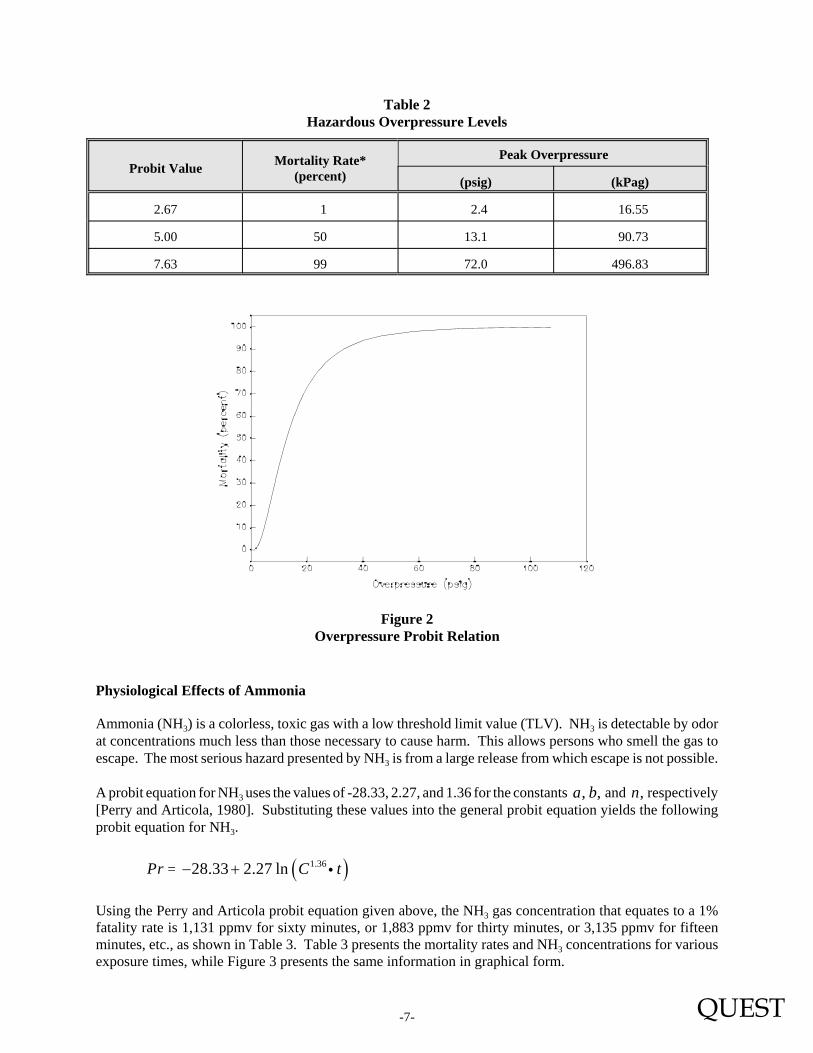
In the event of an ignition and explosion of a flammable gas or gas/aerosol cloud, the overpressure levelsnecessary to cause injury to the public are often defined as a function of peak overpressure. Unlike potentialfire hazards, persons who are exposed to overpressures have no time to react or take shelter; thus, time doesnot enter into the hazard relationship. Work by the Health and Safety Executive, United Kingdom [HSE,1991], has produced a probit relationship based on peak overpressure. This probit equation has the followingform.

=Pr ( )1.47 1.37 ln p+ i

where: = peak overpressure, psigp

Table 2 presents the probit results for 1%, 50%, and 99% fatalities. The graphical form of the overpressureprobit equation is presented in Figure 2.

QUEST-7-

Figure 2Overpressure Probit Relation

Table 2Hazardous Overpressure Levels

Probit Value Mortality Rate*(percent)

Peak Overpressure

(psig) (kPag)

2.67 1 2.4 16.55

5.00 50 13.1 90.73

7.63 99 72.0 496.83

Physiological Effects of Ammonia

Ammonia (NH3) is a colorless, toxic gas with a low threshold limit value (TLV). NH3 is detectable by odorat concentrations much less than those necessary to cause harm. This allows persons who smell the gas toescape. The most serious hazard presented by NH3 is from a large release from which escape is not possible.

A probit equation for NH3 uses the values of -28.33, 2.27, and 1.36 for the constants and respectively, ,a b ,n[Perry and Articola, 1980]. Substituting these values into the general probit equation yields the followingprobit equation for NH3.

= Pr ( )1.3628.33 2.27 ln C t− + i

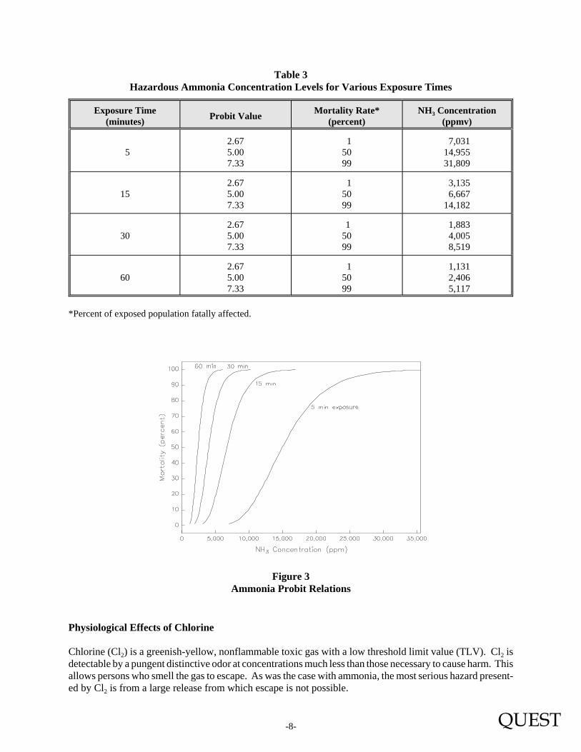
Using the Perry and Articola probit equation given above, the NH3 gas concentration that equates to a 1%fatality rate is 1,131 ppmv for sixty minutes, or 1,883 ppmv for thirty minutes, or 3,135 ppmv for fifteenminutes, etc., as shown in Table 3. Table 3 presents the mortality rates and NH3 concentrations for variousexposure times, while Figure 3 presents the same information in graphical form.

QUEST-8-

Figure 3Ammonia Probit Relations

Table 3Hazardous Ammonia Concentration Levels for Various Exposure Times

Exposure Time(minutes) Probit Value Mortality Rate*

(percent)NH3 Concentration

(ppmv)

52.675.007.33

15099

7,03114,95531,809

152.675.007.33

15099

3,135 6,66714,182

302.675.007.33

15099

1,883 4,005 8,519

602.675.007.33

15099

1,131 2,406 5,117

*Percent of exposed population fatally affected.

Physiological Effects of Chlorine

Chlorine (Cl2) is a greenish-yellow, nonflammable toxic gas with a low threshold limit value (TLV). Cl2 isdetectable by a pungent distinctive odor at concentrations much less than those necessary to cause harm. Thisallows persons who smell the gas to escape. As was the case with ammonia, the most serious hazard present-ed by Cl2 is from a large release from which escape is not possible.

QUEST-9-

A probit equation for Cl2 uses the values of -36.45, 3,13, and 2.64 for the constants and respectively, ,a b ,n[Perry and Articola, 1980]. Substituting these values into the general probit equation yields the followingprobit equation for Cl2.

= Pr ( )2.6436.45 3.13 ln C t− + i

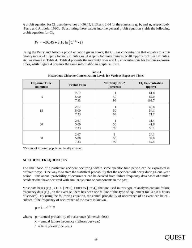
Using the Perry and Articola probit equation given above, the Cl2 gas concentration that equates to a 1%fatality rate is 24.1 ppmv for sixty minutes, or 31.4 ppmv for thirty minutes, or 40.8 ppmv for fifteen minutes,etc., as shown in Table 4. Table 4 presents the mortality rates and Cl2 concentrations for various exposuretimes, while Figure 4 presents the same information in graphical form.

Table 4Hazardous Chlorine Concentration Levels for Various Exposure Times

Exposure Time(minutes) Probit Value Mortality Rate*

(percent)Cl2 Concentration

(ppmv)

52.675.007.33

15099

61.8 82.0108.7

152.675.007.33

15099

40.8 54.1 71.7

302.675.007.33

15099

31.4 41.6 55.1

602.675.007.33

15099

24.1 32.0 42.4

*Percent of exposed population fatally affected.

ACCIDENT FREQUENCIES

The likelihood of a particular accident occurring within some specific time period can be expressed indifferent ways. One way is to state the statistical probability that the accident will occur during a one-yearperiod. This annual probability of occurrence can be derived from failure frequency data bases of similaraccidents that have occurred with similar systems or components in the past.

Most data bases (e.g., CCPS [1989], OREDA [1984]) that are used in this type of analysis contain failurefrequency data (e.g., on the average, there has been one failure of this type of equipment for 347,000 hoursof service). By using the following equation, the annual probability of occurrence of an event can be cal-culated if the frequency of occurrence of the event is known.

=p ( )1 te λ−− i

where: = annual probability of occurrence (dimensionless)p= annual failure frequency (failures per year)λ

= time period (one year)t

QUEST-10-

Figure 4Chlorine Probit Relations

If an event has occurred once in 347,000 hours of use, its annual failure frequency is computed as follows.

= = λ 1 event 8,760 hours347,000 hours year

i 0.0252 events/year

The annual probability of occurrence of the event is then calculated as follows.

= =p ( )0.0252 11 e −− i 0.0249

Note that the frequency of occurrence and the probability of occurrence are nearly identical. (This is alwaystrue when the frequency is low.) An annual probability of occurrence of 0.0249 is approximately the sameas saying there will probably be one event per forty years of use.

Due to the scarcity of accident frequency data bases, it is not always possible to derive an exact probabilityof occurrence for a particular accident. Also, variations from one system to another (e.g., differences indesign, operation, maintenance, or mitigation measures) can alter the probability of occurrence for a specificsystem. Therefore, variations in accident probabilities are usually not significant unless the variationapproaches one order of magnitude (i.e., the two values differ by a factor of ten).

The following subsections describe the basis and origin of failure frequency rates used in this analysis.

Pipeline Failure Rate Data

Department of Transportation (DOT) data for underground liquid pipelines in the United States indicate afailure rate of 1.35 x 10-3 failures/mile/year [DOT, 1988]. Data compiled from DOT statistics on failures ofgas pipelines show a failure rate of 1.21 x 10-3 failures/mile/year for steel pipelines in the United States

QUEST-11-

[Jones, et al., 1986]. In addition to failures of buried pipe, these data include failures of buried pipelinecomponents, such as block valves and check valves, when the failure resulted in a release of fluid from thepipeline.

These data sets are not sufficiently detailed to allow a determination of the failure frequency as a function ofthe size of the release (i.e., the size of hole in the pipeline). However, British Gas has gathered such data ontheir gas pipelines [Fearnehough, 1985]. These data indicate that well over 90% of all failures are less thana one-inch diameter hole, and only 3% are greater than a three-inch diameter hole.

Data compiled from DOT data on gas pipelines in the United States show a trend toward higher failure ratesas pipe diameter decreases [Jones, et al., 1986]. (Smaller diameter pipes have thinner walls; thus, they aremore prone to failure by corrosion and by mechanical damage from outside forces.)

Railcar Failure Rate Data

Railroad accidents can result from a number of causes; track defects, operational errors, train control equip-ment failure (e.g., signaling), etc. For the purposes of the risk analysis, the specific cause of an accident thatresults in a release of product is not specifically required. The use of historic data to define the accident fail-ure rate will be sufficient.

The construction of the QRA will assume a Track Class of 3 (30 mph maximum speed) for the analysis.Track classes range from 1 (10 mph) to 6 (110 mph) according to the Federal Railroad Administration SafetyStandards (49 CFR 213). Class 3 track was assumed to represent track that would be located near mostschools in urban or suburban areas.

The historical data yield a derailment rate of approximately 5.0 x 10-7 derailments per loaded mile for Class3 track [FRA, 1992]. When this derailment rate is combined with the conditional probability that a releaseoccurs from a pressurized rail car (e.g., LPG, Cl2, or NH3) at the rate of 0.08 releases/derailment, the releaseprobability becomes 4.0 x 10-8 releases from a pressurized railcar per loaded mile traveled.

The chance of a BLEVE occurring following a derailment and release of flammable material is determinedby a number of factors: size and duration of the release, ignition of the released material, orientation of theignited jet, and impingement of the flame on the railcar shell. Although we are not aware of specifichistorical data that would provide a probability of BLEVE per loaded mile traveled, for the purposes of thisexample, it was assumed 5% of the flammable pressurized railcar derailments that caused a release of cargoeventually BLEVEd. This results in a railcar BLEVE probability of 2.0 x 10-9 BLEVEs per mile for a loadedLPG railcar.

RISK QUANTIFICATION

Conceptually, performing a risk analysis for each pipeline or railway route near a school site is straight-forward. For example, for releases that involve toxic or flammable materials, the analysis can be divided intothe following steps.

Step 1. Along each section of the pipeline or railway, determine the potential credible releases that wouldcreate a toxic or flammable gas cloud, vapor cloud explosion, torch fire, pool fire, or BLEVE.

Step 2. Determine the probability of occurrence of each of these releases.

QUEST-12-

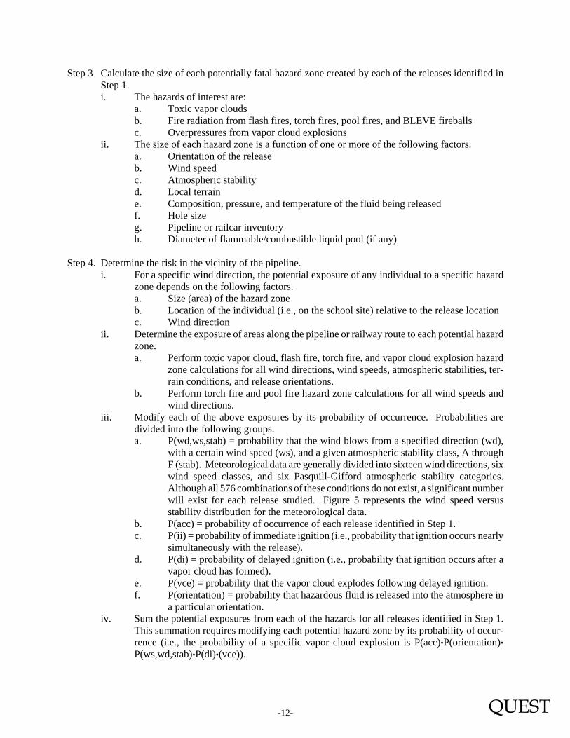
Step 3 Calculate the size of each potentially fatal hazard zone created by each of the releases identified inStep 1.i. The hazards of interest are:

a. Toxic vapor cloudsb. Fire radiation from flash fires, torch fires, pool fires, and BLEVE fireballsc. Overpressures from vapor cloud explosions

ii. The size of each hazard zone is a function of one or more of the following factors.a. Orientation of the releaseb. Wind speedc. Atmospheric stabilityd. Local terraine. Composition, pressure, and temperature of the fluid being releasedf. Hole sizeg. Pipeline or railcar inventoryh. Diameter of flammable/combustible liquid pool (if any)

Step 4. Determine the risk in the vicinity of the pipeline.i. For a specific wind direction, the potential exposure of any individual to a specific hazard

zone depends on the following factors.a. Size (area) of the hazard zoneb. Location of the individual (i.e., on the school site) relative to the release locationc. Wind direction

ii. Determine the exposure of areas along the pipeline or railway route to each potential hazardzone.a. Perform toxic vapor cloud, flash fire, torch fire, and vapor cloud explosion hazard

zone calculations for all wind directions, wind speeds, atmospheric stabilities, ter-rain conditions, and release orientations.

b. Perform torch fire and pool fire hazard zone calculations for all wind speeds andwind directions.

iii. Modify each of the above exposures by its probability of occurrence. Probabilities aredivided into the following groups.a. P(wd,ws,stab) = probability that the wind blows from a specified direction (wd),

with a certain wind speed (ws), and a given atmospheric stability class, A throughF (stab). Meteorological data are generally divided into sixteen wind directions, sixwind speed classes, and six Pasquill-Gifford atmospheric stability categories.Although all 576 combinations of these conditions do not exist, a significant numberwill exist for each release studied. Figure 5 represents the wind speed versusstability distribution for the meteorological data.

b. P(acc) = probability of occurrence of each release identified in Step 1.c. P(ii) = probability of immediate ignition (i.e., probability that ignition occurs nearly

simultaneously with the release).d. P(di) = probability of delayed ignition (i.e., probability that ignition occurs after a

vapor cloud has formed).e. P(vce) = probability that the vapor cloud explodes following delayed ignition.f. P(orientation) = probability that hazardous fluid is released into the atmosphere in

a particular orientation.iv. Sum the potential exposures from each of the hazards for all releases identified in Step 1.

This summation requires modifying each potential hazard zone by its probability of occur-rence (i.e., the probability of a specific vapor cloud explosion is P(acc)•P(orientation)•P(ws,wd,stab)•P(di)•(vce)).

QUEST-13-

Figure 5Example Wind Speed/Atmospheric Stability Categories

RISK ANALYSIS RESULTS

Individual Risk Transects

Individual risk transects (risk as function of distance from the pipeline or railway) were constructed for thefour example pipelines and three example railcar cargoes. Examples from the following scenarios arepresented in this section of the report.

• release from a 30-inch, 1,000 psig, natural gas transmission pipeline• release from a 12-inch, 700 psig, natural gas distribution pipeline• release from an 8-inch, 450 psig, LPG transmission pipeline• release from a 6-inch, 330 psig, anhydrous ammonia transmission pipeline• derailment and release from an LPG railcar, 33,000-gallon capacity• derailment and release from an anhydrous ammonia railcar, 33,000-gallon capacity• derailment and release from a chlorine railcar, 90-ton capacity

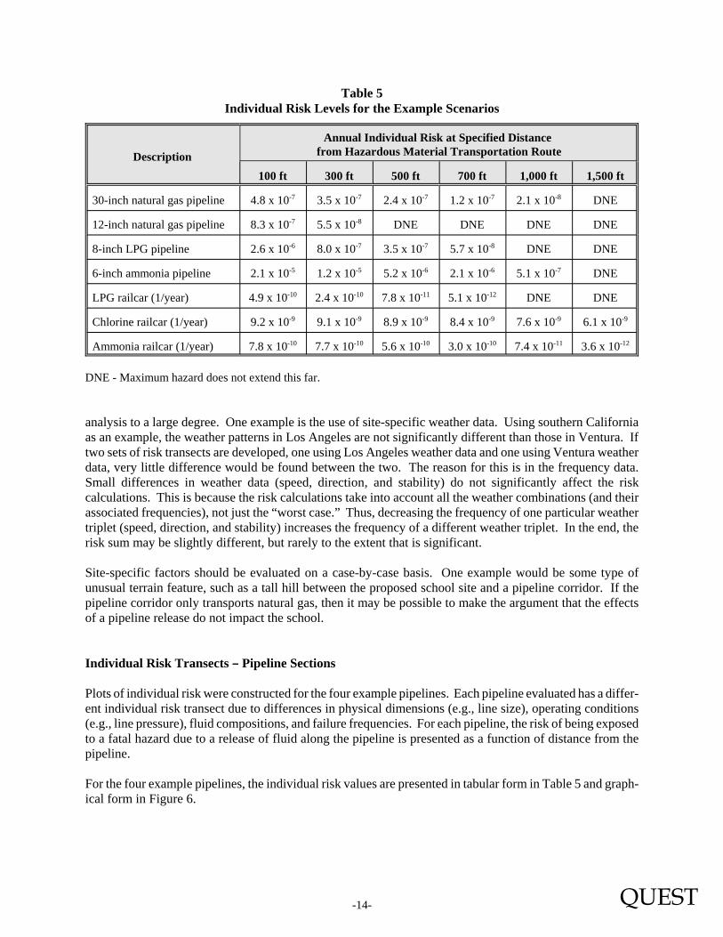
Individual risk calculations present levels of risk based on annual exposure. For any risk level identified ata specific location, that level of risk is based (conservatively) upon one’s presence 24 hours a day, 365 daysper year. The meaning of a particular value of risk at a location is related to the hazards that are modeled andtheir probability. For example, if an individual in the vicinity of a pipeline is at a location that correspondsto a 1.0 x 10-6 risk level, then his risk from being fatally affected by any one of the potential releases fromthat pipeline is one chance in one million per year. At a location closer to the pipeline, the risk is higher, andfarther away from the pipeline, the risk is lower. Table 5 presents the individual risk levels found at specificdistances from the seven example pipeline and railcar scenarios. For the railcar scenarios, the calculated riskis based on one (1) loaded railcar passing by the location per year. To adjust for the true number of railcarspassing by a site, the number of railcars per year is simply multiplied by the individual risk level.

There are several site-specific factors that can affect the final risk values that are calculated. In most cases,the site-specific factors will only affect portions of the analysis and thus will not be able to influence the

QUEST-14-

Table 5Individual Risk Levels for the Example Scenarios

DescriptionAnnual Individual Risk at Specified Distance

from Hazardous Material Transportation Route

100 ft 300 ft 500 ft 700 ft 1,000 ft 1,500 ft

30-inch natural gas pipeline 4.8 x 10-7 3.5 x 10-7 2.4 x 10-7 1.2 x 10-7 2.1 x 10-8 DNE

12-inch natural gas pipeline 8.3 x 10-7 5.5 x 10-8 DNE DNE DNE DNE

8-inch LPG pipeline 2.6 x 10-6 8.0 x 10-7 3.5 x 10-7 5.7 x 10-8 DNE DNE

6-inch ammonia pipeline 2.1 x 10-5 1.2 x 10-5 5.2 x 10-6 2.1 x 10-6 5.1 x 10-7 DNE

LPG railcar (1/year) 4.9 x 10-10 2.4 x 10-10 7.8 x 10-11 5.1 x 10-12 DNE DNE

Chlorine railcar (1/year) 9.2 x 10-9 9.1 x 10-9 8.9 x 10-9 8.4 x 10-9 7.6 x 10-9 6.1 x 10-9

Ammonia railcar (1/year) 7.8 x 10-10 7.7 x 10-10 5.6 x 10-10 3.0 x 10-10 7.4 x 10-11 3.6 x 10-12

DNE - Maximum hazard does not extend this far.

analysis to a large degree. One example is the use of site-specific weather data. Using southern Californiaas an example, the weather patterns in Los Angeles are not significantly different than those in Ventura. Iftwo sets of risk transects are developed, one using Los Angeles weather data and one using Ventura weatherdata, very little difference would be found between the two. The reason for this is in the frequency data.Small differences in weather data (speed, direction, and stability) do not significantly affect the riskcalculations. This is because the risk calculations take into account all the weather combinations (and theirassociated frequencies), not just the “worst case.” Thus, decreasing the frequency of one particular weathertriplet (speed, direction, and stability) increases the frequency of a different weather triplet. In the end, therisk sum may be slightly different, but rarely to the extent that is significant.

Site-specific factors should be evaluated on a case-by-case basis. One example would be some type ofunusual terrain feature, such as a tall hill between the proposed school site and a pipeline corridor. If thepipeline corridor only transports natural gas, then it may be possible to make the argument that the effectsof a pipeline release do not impact the school.

Individual Risk Transects B Pipeline Sections

Plots of individual risk were constructed for the four example pipelines. Each pipeline evaluated has a differ-ent individual risk transect due to differences in physical dimensions (e.g., line size), operating conditions(e.g., line pressure), fluid compositions, and failure frequencies. For each pipeline, the risk of being exposedto a fatal hazard due to a release of fluid along the pipeline is presented as a function of distance from thepipeline.

For the four example pipelines, the individual risk values are presented in tabular form in Table 5 and graph-ical form in Figure 6.

QUEST-15-

Figure 6Risk Transects for the Example Pipelines

The following observations can be made from Figure 6.

(a) If an individual were continuously standing on top of the 12-inch natural gas pipeline for one year,he would have a slightly greater than 1.0 x 10-6 (one in one million) chance of being killed by arelease from the pipeline during that year. The release could be from a corrosion hole, puncture, or

rupture of the line that resulted in a continuous gas fire, flash fire, or vapor cloud explosion. Asimilar result can be drawn from the three other pipeline risk transects.

(b) As distance from the pipeline increases, the risk of fatality due to a release from any one of the pipe-lines decreases.

(c) At distances greater than about 400 feet from the 12-inch natural gas pipeline, there are no lethalhazard impacts; thus, the risk of fatality due to releases from the pipeline falls to zero. The same istrue for the LPG pipeline at distances greater than about 1,000 feet; greater than about 1,200 feet forthe 30-inch natural gas line; and greater than 1,400 feet for the anhydrous ammonia pipeline.

Individual Risk Transects - Railway Lines

The base cases for the individual risk transects for the railway lines are calculated assuming one loaded railcarpasses by the school site per year. Risk transects for the three example rail cargoes are presented in Figure7. A review of Figure 7 reveals the following.

(a) The risk of being fatally affected by a release from a chlorine railcar (one passing railcar per year)is approximately 9.0 x 10-9 near the rail line and decreases very little out to 1,500 feet from the railline. This is due to the long distances traveled by chlorine gas in a potentially lethal concentration.Large releases can extend much farther than the 1,500 foot distance set by the regulations.

QUEST-16-

Figure 7Risk Transects for the Three Example Rail

Cargoes (1 railcar/year)

(b) Peak risk levels from one loaded ammonia or LPG railcar per year are approximately 8.0 x 10-10 nearthe railway and decrease significantly as distance from the railway increases.

(c) At distances greater than about 1,000 feet from the rail line, there are no lethal LPG railcar hazardimpacts (hazards are nonlethal at this distance), and thus no risk of fatality due to releases from anLPG railcar. Hazards for ammonia and chlorine railcar releases extend well past the 1,500 foot cutoffdistance.

If we compare the risk transects for the LPG pipeline and LPG railcar, we see that the shapes of the curvesare similar, which shows that the hazards from a pipeline release and from a damaged railcar are similar. But,there is a considerable difference in the frequency of these events. If we compare the peak risk (the risk ontop of the pipeline or on the rail line), the pipeline is about 6,500 times as likely to create a fatal hazard thanthe one railcar that passes by each year. This means that it would take about 6,500 railcars per year passingby the school site to create the same risk as the pipeline. The total LPG railcar risk is a simple multiplicationof the number of railcars and the previously calculated risk for one railcar per year. So once the true numberof LPG railcars passing by the school site in one year is known, the risk transect can be adjusted to reflectthe true total risk.

Application of Risk Transects to School Siting

The development of a range of pipeline and railcar risk transects provides a consistent approach to evaluatingthe potential risk to a proposed school location. Since the pipeline and railcar risk transects are independent,their individual contributions are additive when evaluating the total risk to a proposed school location. Thisis best demonstrated by a series of examples.

QUEST-17-

Example 1. Proposed School Site is Located 330 Feet from a 30-inch Natural Gas TransmissionPipeline

A review of Table 5 and Figure 6 would indicate that the individual risk at the school site is approximately3.3 x 10-7/year.

Using an individual risk acceptability standard of 1.0 x 10-6 fatality/year (one chance in one million per yearof being fatally affected by a release from the pipeline) would indicate that the school site is within (below)the acceptable range.

Example 2. Proposed School Site is Located 330 Feet from a 30-inch Natural Gas TransmissionPipeline and an 8-inch LPG Pipeline Laid in the Same Corridor

Using the data presented in Table 5 and the risk transects for the individual pipelines (Figure 6), it can be seenthat neither pipeline individually produces a risk level above 1.0 x 10-6 per year at the school site. However,when contributions from the two pipelines are summed, the risk level at the school site becomes 1.03 x 10-6.If the acceptable limit is 1.0 x 10-6, this site would not be deemed acceptable. A more detailed analysis togenerate a better estimate of the true risk may be required for this site.

Example 3. Proposed School Site is Located 850 Feet from a Railway

A railway runs near the boundary of the proposed school site. Rail officials have provided the followinginformation about the recent rail activity along the railway section by the school site for the three examplecargoes.

1,335 loaded LPG railcars per year240 loaded NH3 railcars per year43 loaded Cl2 railcars per year

Using this activity data, the risk transects for the three example cargoes can be constructed. These are pre-sented in Figure 8, along with a summation risk transect. The summation transect represents the risk fromall three cargoes at any distance from the rail line. As can be seen from the figure, the proposed school siteat 850 feet from the railway would be acceptable using the 1.0 x 10-6 criteria. If the school were within 250feet of the railway, the combined risk from the three rail-transported commodities would not be acceptable.

Example 4. Proposed School Site is Located Near a Pipeline Corridor and a Railway

In some cases, such as the example in Figure 9, a school site may be proposed in a location that can beaffected by both pipeline and railcar releases. In this event, the impacts of one transportation mode on theother are assumed to be independent and the potential risks are additive. In the example calculation, thepipeline corridor (with a 30-inch natural gas distribution line and a 6-inch anhydrous ammonia line) is located900 feet from the edge of the school property. On the other side of the school site is a railway (1,040 feetfrom the nearest school boundary), with the following annual activity.

522 loaded LPG railcars per year95 loaded NH3 railcars per year36 loaded Cl2 railcars per year

QUEST-18-

Figure 8Risk Transects for the Railway in Example 3

Figure 9Area Surrounding the Proposed School Site

for Example 4

The risk data for the school site are presented in Table 6. The summation of risk from all five sources iscalculated for the northeastern most point of the school property. This is the location on the proposed sitethat will experience the highest individual risk level. All other locations at the site will be at a greater

QUEST-19-

distance from the pipeline corridor, the rail line, or both, so the individual risk will be lower. Based on the1.0 x 10-6 acceptability criteria, this proposed site would not be deemed acceptable.

Table 6Individual Risk Values for Example 4

DescriptionDistance from Hazardous

Material Transportation Route(ft)

Annual Individual Risk

30-inch natural gas pipeline 900 3.99 x 10-8

6-inch ammonia pipeline 900 8.09 x 10-7

LPG railcar (522/year) 1,040 0

Chlorine railcar (36/year) 1,040 2.69 x 10-7

Ammonia railcar (95/year) 1,040 5.49 x 10-9

Summation of all hazards, valid only at northeast corner of theproposed school property 1.12 x 10-6

* 1,040 feet is beyond the extent of all lethal hazards from railcar releases.

SUMMARY

A method has been developed that provides a consistent and defensible approach for evaluating the potentialimpact of hazardous material pipelines and railcar cargoes on potential school sites. The methodology satis-fies the State of California’s Code of Regulations for evaluating potential schools sites. In addition, becauseof the modular nature of the methodology, additional pipeline systems and railcar cargoes can be added tothe system. If it were to become necessary, road transportation routes and cargoes could easily be added tothe system since the procedure for developing roadway risk transects would be similar to that used for therailway risk transects.

The results of risk transect calculations (risk versus distance) can easily be incorporated into a simple spread-sheet program where site-specific modifiers, such as distance from the pipeline or railway to the school site,number of railcar cargoes, etc., would be input parameters. Such an approach would allow the system to beused throughout the school system network and avoid the widely varying results currently generated by quali-tative analyses.

REFERENCES

Baker, Q. A., M. J. Tang, E. Scheier, and G. J. Silva (1994), “Vapor Cloud Explosion Analysis.” Presentedat the 28th Loss Prevention Symposium, American Institute of Chemical Engineers (AIChE), April 17-21,1994.

Baker, Q. A., C. M. Doolittle, G. A. Fitzgerald, and M. J. Tang (1998), “Recent Developments in the Baker-Strehlow VCE Analysis Methodology.” Process Safety Progress, 1998: p. 297.

QUEST-20-

CCPS (1989), Guidelines for Process Equipment Reliability Data, with Data Tables. Center for ChemicalProcess Safety of the American Institute of Chemical Engineers, 345 East 47th Street, New York, NewYork, 1989.

Chang, Joseph C., Mark E. Fernau, Joseph S. Scire, and David G. Strimaitis (1998), A Critical Review ofFour Types of Air Quality Models Pertinent to MMS Regulatory and Environmental Assessment Missions.Mineral Management Service, Gulf of Mexico OCS Region, U.S. Department of the Interior, NewOrleans, November, 1998.

DOT (1988), Hazardous Materials Information System. U.S. Department of Transportation, Materials Trans-portation Bureau, Washington, D.C., 1988.

Fearnehough, G. D. (1985), The Control of Risk in Gas Transmission Pipelines. British Gas Research andDevelopment, D.473, January, 1985.

FRA (1992), Railroad Accident/Incident Database, 1992. U.S. Federal Railroad Administration, Office ofSafety, 400 7th Street S.W., Washington, D.C., 20590, 1992.

Hanna, S. R., D. G. Strimaitis, and J. C. Chang (1991), Hazard Response Modeling Uncertainty (A Quantita-tive Method), Volume II, Evaluation of Commonly-Used Hazardous Gas Dispersion Models. Study co-sponsored by the Air Force Engineering and Services Center, Tyndall Air Force Base, Florida, and theAmerican Petroleum Institute; performed by Sigma Research Corporation, Westford, Massachusetts,September, 1991.

HSE (1991), Major Hazard Aspects of the Transport of Dangerous Substances. Health and Safety Executive,Advisory Committee on Dangerous Substances, London, United Kingdom, 1991

Jones, D. J., G. S. Kramer, D. N. Gideon, and R. J. Eiber (1986), An Analysis of Reportable Incidents forNatural Gas Transmission and Gathering Lines, 1970 through June 1984. Prepared for the PipelineResearch Committee, American Gas Association, NG-18, Report No. 158, March, 1986.

OREDA (1984), OREDA, Offshore Reliability Data Handbook (First Edition). OREDA, Post Office Box370, N-1322 Hovik, Norway, 1984.

Perry, W. W., and W. P. Articola (1980), “Study to Modify the Vulnerability Model of the Risk ManagementSystem.” U.S. Coast Guard, Report CG-D-22-80, February, 1980.

TRC (1991), Evaluation of Dense Gas Simulation Models. Prepared for the U.S. Environmental ProtectionAgency by TRC Environmental Consultants, Inc., East Hartford, Connecticut 06108, EPA Contract No.68-02-4399, May, 1991.

Tsao, C. K., and W. W. Perry (1979), Modifications to the Vulnerability Model: A Simulation System forAssessing Damage Resulting from Marine Spills. U.S. Coast Guard Report CG-D-38-79, Washington,D.C., March, 1979.