University of South FloridaScholar Commons

Graduate Theses and Dissertations Graduate School

11-5-2008

Application of Remote Sensing Methods to Assessthe Spatial Extent of the Seagrass Resource in St.Joseph Sound and Clearwater Harbor, Florida,U.S.A.Cynthia A. MeyerUniversity of South Florida

Follow this and additional works at: https://scholarcommons.usf.edu/etd

Part of the American Studies Commons

This Thesis is brought to you for free and open access by the Graduate School at Scholar Commons. It has been accepted for inclusion in GraduateTheses and Dissertations by an authorized administrator of Scholar Commons. For more information, please contact scholarcommons@usf.edu.

Scholar Commons CitationMeyer, Cynthia A., "Application of Remote Sensing Methods to Assess the Spatial Extent of the Seagrass Resource in St. Joseph Soundand Clearwater Harbor, Florida, U.S.A." (2008). Graduate Theses and Dissertations.https://scholarcommons.usf.edu/etd/405

Application of Remote Sensing Methods to Assess the Spatial Extent of the

Seagrass Resource in St. Joseph Sound and Clearwater Harbor, Florida, U.S.A.

by

Cynthia A. Meyer

A thesis submitted in partial fulfillment of the requirements for the degree of

Master of Arts Department of Geography

College of Arts and Sciences University of South Florida

Major Professor: Ruiliang Pu, Ph.D. Susan S. Bell, Ph.D.

Steven Reader, Ph.D.

Date of Approval: November 5, 2008

Keywords: Landsat TM, Maximum Likelihood, Mahalanobis Distance, GIS, Gulf of Mexico

© Copyright 2008, Cynthia A. Meyer

Dedication

This thesis is dedicated to my pack.

"So long, and thanks for all the fish." - Hitchhikers Guide to the Galaxy

Acknowledgements

Pinellas County Watershed Management Division

Kris Kaufman, Southwest Florida Water Management District

Dr. Bob Muller & Dr. Behzad Mahmoudi, Florida Marine Research Institute

Dr. Bell & Dr. Reader, University of South Florida

Dr. Ruiliang Pu, University of South Florida, 谢谢您的帮助

i

Table of Contents

List of Tables iii List of Figures iv Abstract vi Chapter One: Introduction 1

1.1 Background 1 1.2 Goal 1 1.3 Objectives 2 1.4 Description of Study Area 3

Chapter Two: Literature Review 7

2.1 Seagrass 7 2.1.1 Seagrass Resource Ecology 7 2.1.2 Seagrass Assessment Methods 8 2.2 Remote Sensing Applications 9

2.2.1 Landsat Imagery 11 2.2.2 Aerial Photography 13

2.3 Remote Sensing Classification 13 2.3.1 Imagery Classification 13 2.3.2 Hard Classification Methods 14 2.3.3 Soft Classification Methods 15

Chapter Three: Methodology 16

3.1 Methodology Overview 16 3.2 Data Sources 16

3.2.1 Remote Sensing Data Sources 16 3.2.1.1 Aerial Photointerpretation SAV Mapping 16 3.2.1.2 Satellite Imagery 19

3.2.2 Field Survey Data 21 3.2.2.1 Seagrass Monitoring Data 21 3.2.2.2 Water Quality Monitoring Data 23

3.3 Landsat 5 TM Imagery Analysis 25 3.3.1 Imagery Preprocessing 25

3.3.2 Imagery Classification 27 3.3.3 Classification Accuracy Analysis 33

ii

3.4 Analyses 33 3.4.1 Comparison to Existing Maps 33 3.4.2 Ability to Map SAV Variation 34

Chapter Four: Results and Discussion 35

4.1 Classification Results 35 4.1.1 Unsupervised Classification 35 4.1.2 Supervised Classification 37

4.1.2.1 Hard Classification 37 4.1.2.1.1 Presence/Absence of SAV 37 4.1.2.1.2 Estimated Coverage of SAV 41

4.1.2.2 Soft Classification 46 4.1.2.2.1 Artificial Neural Networks 46 4.1.2.2.2 Linear Spectral Unmixing 48

4.2 Assessment of Classification Methods 50 4.2.1 Accuracy Comparison of SAV Maps 50

4.2.3 Spatial Comparison of SAV Maps 53 4.2.4 Ability to Map SAV Variation 58

Chapter Five: Conclusions 60 References Cited 62

iii

List of Tables Table 1: Landsat 5 TM band descriptions. 12 Table 2: Landsat 5 TM image details. 19 Table 3: Radiometric resolution descriptive statistics calculated for the

ROI training data. 30 Table 4: Accuracy estimates for the supervised classification methods. 39 Table 5: Supervised classification commission and omission errors,

and producer and user’s accuracy. 39 Table 6: Validation for classification methods SAV presence/absence. 39 Table 7: Accuracy estimates for the supervised classification methods. 43 Table 8: Supervised Classification commission and omission errors,

and producer and user’s accuracy. 43 Table 9: Validation for classification methods SAV estimated coverage 43 Table 10: Comparison of validation for classification methods 52 Table 11: Area calculated for each classification method. 54 Table 12: Aerial Photointerpretation versus Mahalanobis Distance

Classification. 56 Table 13: Aerial Photointerpretation versus Maximum Likelihood

Classification. 57 Table 14: Potential variation associated with the estimated accuracies

for the classification methods. 58

iv

List of Figures Figure 1: Location of the study site. 3 Figure 2: Study area includes St. Joseph Sound and Clearwater Harbor. 4 Figure 3: Seagrass species found in the study area. 5 Figure 4: Rhizophytic algae and Bay Scallops found in the study area. 5 Figure 5: Aerial photointerpretation SAV map based on 2006 aerial

imagery. 18 Figure 6: Landsat 5 TM satellite image from May 2, 2006. 20 Figure 4: Pinellas County seagrass monitoring program results for

Clearwater Harbor and St. Joseph Sound. 22 Figure 8: Observed SAV at the Pinellas County Ambient Water Quality

sampling sites for 2005 - 2007. 24 Figure 9: Landsat 5 TM imagery clipped to the study area from 2 May

2006. 26 Figure 10: Mask delineated from band 4 (near infrared). 27 Figure 11: Landsat 5 TM image enhancement using Equalization

function. 28 Figure 12: Histograms of the radiometric resolution of the ROI classes:

No SAV, Patchy SAV and Continuous SAV for TM 1 (A), TM 2 (B), and TM 3 (C). 31

Figure 13: Unsupervised ISODATA classification of Landsat 5 TM image

with environmentally relevant labels. 36 Figure 14: Supervised classification of Landsat 5 TM image using the

Mahalanobis Distance and Maximum Likelihood methods. 38

v

Figure 15: Differences (red circle) between the supervised classifications of Landsat 5 TM image using the Mahalanobis Distance and Maximum Likelihood methods. 40

Figure 16: Supervised classification of Landsat 5 TM image using the

Mahalanobis Distance and Maximum Likelihood methods. 42 Figure 17: Differences (red circle) between the supervised classifications

of Landsat 5 TM image using the Mahalanobis Distance and Maximum Likelihood methods. 44

Figure 18: Differences (red rectangle) between the supervised

classifications of Landsat 5 TM image using the Mahalanobis Distance and Maximum Likelihood methods. 45

Figure 19: Artificial neural network classification of Landsat 5 TM image. 47 Figure 20: Linear spectral unmixing of Landsat 5 TM image. 49 Figure 21: Comparison of validation data to the SAV Aerial

Photointerpretation Map, 2006. 50 Figure 22: Estimated classification accuracies derived from validation

analysis for different classification methods. 53 Figure 23: Discrepancies between the AP and MDC for the

presence/absence of SAV. 56 Figure 24: Discrepancies between the AP and MLC for the estimated

coverage of SAV. 57

vi

Application of Remote Sensing Methods to Assess the Spatial Extent of the Seagrass Resource in St. Joseph Sound and Clearwater Harbor, Florida, U.S.A.

Cynthia A. Meyer

ABSTRACT

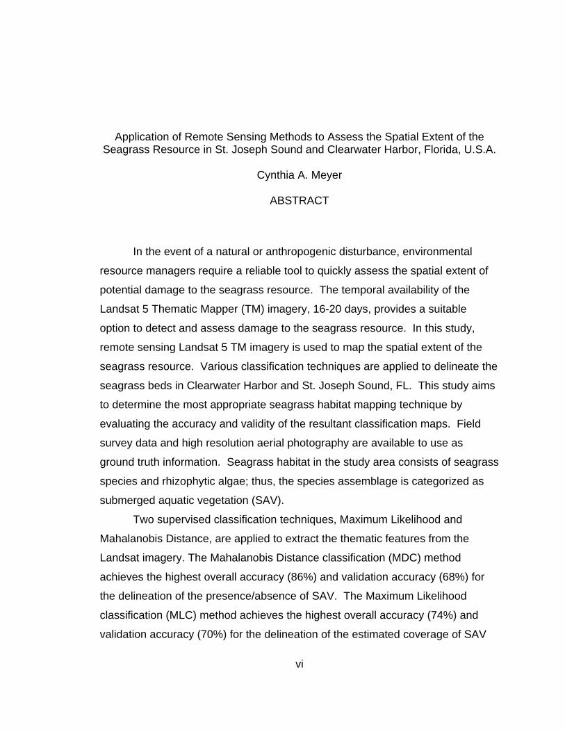
In the event of a natural or anthropogenic disturbance, environmental

resource managers require a reliable tool to quickly assess the spatial extent of

potential damage to the seagrass resource. The temporal availability of the

Landsat 5 Thematic Mapper (TM) imagery, 16-20 days, provides a suitable

option to detect and assess damage to the seagrass resource. In this study,

remote sensing Landsat 5 TM imagery is used to map the spatial extent of the

seagrass resource. Various classification techniques are applied to delineate the

seagrass beds in Clearwater Harbor and St. Joseph Sound, FL. This study aims

to determine the most appropriate seagrass habitat mapping technique by

evaluating the accuracy and validity of the resultant classification maps. Field

survey data and high resolution aerial photography are available to use as

ground truth information. Seagrass habitat in the study area consists of seagrass

species and rhizophytic algae; thus, the species assemblage is categorized as

submerged aquatic vegetation (SAV).

Two supervised classification techniques, Maximum Likelihood and

Mahalanobis Distance, are applied to extract the thematic features from the

Landsat imagery. The Mahalanobis Distance classification (MDC) method

achieves the highest overall accuracy (86%) and validation accuracy (68%) for

the delineation of the presence/absence of SAV. The Maximum Likelihood

classification (MLC) method achieves the highest overall accuracy (74%) and

validation accuracy (70%) for the delineation of the estimated coverage of SAV

vii

for the classes of continuous and patchy seagrass habitat. The soft classification

techniques, linear spectral unmixing (LSU) and artificial neural network (ANN),

did not produce reasonable results for this particular study.

The comparison of the MDC and MLC to the current Seagrass Aerial

Photointerpretation (AP) project indicates that the classification of SAV from

Landsat 5 TM imagery provides a map product with similar accuracy to the AP

maps. These results support the application of remote sensing thematic feature

extraction methods to analyze the spatial extent of the seagrass resource. While

the remote sensing thematic feature extraction methods from Landsat 5 TM

imagery are deemed adequate, the use of hyperspectral imagery and better

spectral libraries may improve the identification and mapping accuracy of the

seagrass resource.

1

Chapter 1

Introduction

1.1 Background As essential nearshore aquatic habitat of the Gulf of Mexico, St. Joseph

Sound and Clearwater Harbor require the development and implementation of

management plans to protect and sustain the ecosystem. The environmental

resources include an extensive seagrass resource, macroalgae habitat,

mangroves, and tidal flats. Understanding the spatial and temporal scales of the

physical substrate is crucial to the assessment of the ecosystem resource status,

structures and functions. The application of remote sensing methods may

enhance the results from the current field survey monitoring programs and the

comprehensive management strategy for the resource. The sustainable

management requires an understanding of the seagrass spatial distribution and

characterization to create accurate habitat maps. Determining the status of the

seagrass resource requires a comprehensive analysis of the geographic extent,

composition, health, and abundance of the submerged aquatic vegetation (SAV)

in the study area. The current monitoring programs provide data on a limited

geographic scale which can not be extrapolated across the entire resource. In

turn, the results of the current studies can not provide a comprehensive resource

trend analysis or appropriate statistical power.

1.2 Goal The purpose of this research is to determine the feasibility of using remote

sensing image data to delineate the spatial extent of the seagrass resource.

Evaluating the accuracy of the classification maps allows the comparison of the

study results to the existing aerial photointerpretation SAV maps. The potential

2

to use Landsat 5 TM imagery as a data source greatly improves the temporal

scale for analyzing spatial changes in the seagrass. In turn, the analyses provide

more frequent information to the environmental resource managers and aid in the

development of resource preservation and protection strategies.

1.3 Objectives Objective One: To create hard classification maps delineating the

presence/absence and estimated coverage of seagrass resource from Landsat

TM imagery using Maximum Likelihood classification (MLC) and Mahalanobis

Distance classification (MDC) techniques.

Objective Two: To create soft classification maps delineating the

presence/absence and estimated coverage of seagrass resource from Landsat

TM imagery using a linear spectral unmixing (LSU) and non-linear artificial neural

network (ANN) algorithms.

Objective Three: To determine the most appropriate classification mapping

technique for the seagrass resource by evaluating the accuracy and validity of

the resulting classification maps.

Objective Four: Determine the ability for change detection by each appropriate

classification method.

3

1.4 Description of Study Area

Approximately 30 kilometers north of the mouth of Tampa Bay (Figure 1),

the area consists of open water regions bounded east and west by the coastal

mainland shoreline and the barrier island chain, respectively. The study area for

this project, St. Joseph Sound and Clearwater Harbor, occurs along the

northwestern coastline of Pinellas County (Figure 2). Of the 95 km2 in the study

area, expansive seagrass beds cover nearly 56 km2 providing essential habitat

for the marine flora and fauna (Kaufman, 2007). In comparison, the study area

has seagrass acreage equivalent to 60% of the total seagrass acreage found in

the entire Tampa Bay estuary. Concluded from the results of the seagrass aerial

mapping project (Kaufman, 2007), the seagrass acreage in the study area has

increased slightly since the program began in 1998 (Meyer and Levy, 2008;

Kaufman, 2007).

Figure 1. Location of the study site.

4

Figure 2. Study area includes St. Joseph Sound and Clearwater Harbor

The ecosystem of the study area provides critical bird nesting areas,

sessile algal communities, essential fishery habitats, marine mammal and turtle

habitats, and numerous recreational opportunities. The prominent seagrass

species consist of Syringodium filiforme, Thalassia testudinum, and Halodule

wrightii (Figure 3). In addition to the seagrass species, the SAV includes a variety

of rhizophytic algae. Figure 4 shows seven rhizophytic algae and an invertebrate

common in Clearwater Harbor and St. Joseph Sound. The habitat also hosts a

plethora of invertebrates including the Bay Scallop (Argopecten irradians) (Meyer

and Levy, 2008).

5

Figure 3. Seagrass species found in the study area.

Figure 4. Rhizophytic algae and Bay Scallops found in the study area.

6

The water quality in the study area is relatively good in comparison to the

Tampa Bay area (Levy et al., 2008). Transmissivity, measured at 660 nm, is a

measurement of the percentage of light that can pass through the water. The

mean transmissivity in the study area ranges from 90-95% (Levy et al., 2008).

This level of water clarity should be suitable for the use of the satellite imagery.

Anthropogenic and natural stresses impact the health, sustainability, and

persistence of the aquatic ecosystem (Short et al., 2001). Correlated with

urbanization, anthropogenic factors such as stormwater pollution, hardened

shorelines, development, eutrophication, and boat propeller scarring cause direct

and indirect damages to the nearshore habitats (Meyer and Levy, 2008). Man-

made features in the study area include dredge and fill operations, boat

channels, spoil islands, finger canal systems, seawalls, and causeways. In turn,

natural factors such as water circulation, beach erosion, climate change, and

weather events may also cause changes to occur in the ecosystem. The

complexity of the interacting anthropogenic and natural conditions adds to the

intricate dynamics of Clearwater Harbor and St. Joseph Sound. These

interacting environmental issues present a challenge for resource managers to

develop strategies to protect and sustain the quality of the ecosystem (Meyer and

Levy, 2008).

7

Chapter 2

Literature Review 2.1 Seagrass 2.1.1 Seagrass Resource Ecology

Seagrasses are flowering plants, angiosperms, specialized for living in

marine nearshore environments (Short et al., 2001). Areas containing dense

populations of seagrasses are considered a seagrass resource. Ecological

functions provided by seagrass resource include structural and physiological

characteristics that support species living in the seagrass communities.

Functions such as nutrient cycling, detritus production, sediment formation, and

shelter increase the primary productivity of the ecosystem (Dawes et. al., 2004).

Seagrass beds grow as continuous meadows or a mosaic of various size and

shape patches (Brooks and Bell, 2001). Along the central Florida coast of the

Gulf of Mexico, the seagrass growing season is May-September (Avery and

Johansson, 2001) which coincides with the findings of Robbins and Bell (2000)

reporting the greater changes in seagrass spatial extent from the spring to the fall

seasons. Other factors such as physiology, growth characteristics, including

water depth and salinity gradients may contribute to the spatial distribution of the

seagrass beds (Robbins and Bell, 2000).

Seagrass requires available light for photosynthesis (Short et al., 2001),

and the depth penetration of the available light is correlated with seagrass growth

and survival (Dennison et al., 1993). Thus, good water clarity is crucial to the

persistence and growth of the seagrass beds. The health of the seagrass

resource may also be an indicator of water clarity and nutrient levels (Dennison

et al., 1993). Disturbances in the water quality such as nitrification, sediment

suspension, and pollution can negatively affect water quality and light penetration

8

(Levy et al., 2008). Correlated with urbanization, there is an increase of

anthropogenic disturbances to seagrass resources (Tomasko et al., 2005).

Environmental managers acknowledge the relationship between the

anthropogenic factors and the degradation of the seagrass resource and realize

the importance of sustaining this valuable ecosystem (Chauvaud et al., 1998).

Currently, coastal habitat maps including seagrass areas provide essential

information for management and planning decisions (Mumby et al., 1999). The

sustainable management requires an understanding of the seagrass spatial

distribution and characterization.

2.1.2 Seagrass Assessment Methods

Resource managers and researchers implement various techniques to

assess and monitor the spatial and temporal changes of the seagrass habitat.

Kirkman (1996) describes some of the methods for seagrass monitoring. The

most common field survey technique consists of permanent transect monitoring.

Usually monitored annually, transects are revisited by using spatial coordinates

from a Global Positioning System. In most cases, the permanent transects start

on or near shore and then continue perpendicular to the shoreline (Kirkman,

1996). After arriving on site and locating the transect 0m mark, samplers swim

along the transect line with a meter square frame collecting data on seagrass

species, condition, abundance, and biomass. Other field survey methods include

collecting random point data, stratified random sampling designs (Meyer and

Levy, 2008), and seagrass habitat classification mapping (Kaufman, 2007). The

latter is the most intensive method which requires researchers to swim the entire

seagrass area (Mumby et al., 1999).

In a quest to assess the geographic extent of the seagrass resource,

researchers investigate the use of aerial photography for developing habitat

maps. Historical aerial photography provides coarse baselines for the seagrass

resource extent making it possible to compare the current geographic extent of

the seagrass beds to the previous state. Currently, the analysis of aerial

9

photography supplies seagrass acreage maps to track the spatial and temporal

trends for resource management (Kaufman, 2007). Using digital aerial

photography for seagrass mapping requires the acquisition of large scale

airborne photographs. The resolution of the images typically ranges from 1

meter to 10 meter (Jensen, 2005). Variables such as water clarity and depth can

interfere with the ability of the photo-interpreters to accurately delineate the

seagrass meadows (Kaufman, 2007).

Coastal managers require reliable data to protect and manage ecosystems

(Mumby et al., 1999). Ecological management traditionally relies on small

sample designs and extrapolation of results to larger areas. This practice tends

to ignore the spatial dimension and connectivity of ecosystems (Schmidt and

Skidmore, 2003). Detailed habitat maps aid in the assessment and monitoring of

changes within the seagrass meadows. Seagrass biomass responds quickly to

environmental disturbances and alterations (Short et al., 2001). Usually, these

changes are large enough for detection by remote sensing techniques. In

conjunction with field survey monitoring, remote sensing maps can help provide a

better understanding of the extent of spatial and temporal trends in the seagrass

resource based on their synoptic and frequent characteristics.

2.2 Remote Sensing Applications Remote sensing refers to a form of measurement where the observer is

not in direct contact with the object of study (Coastal Remote Sensing, 2006).

Two main types of remote sensing data collection include active and passive

systems. Active systems generate a source of illumination such as sound or

light (Jensen, 2005). Passive systems rely on the reflected sunlight and emitted

energy from targets to acquire data (Jensen, 2005). Technologies such as aerial

photography, multispectral satellite imagery, and hyperspectral imagery also

record how the sunlight reflects and refracts and radiance emits from targets

(Jensen, 2005). Multispectral imagery expands the classification abilities and

mapping of aerial photointerpretation. Multispectral imagery is usually satellite

10

based and collects less than 10 spectral bands, and requires analysis and

characterization to evaluate the features (Mumby et al., 1999). The spectral

resolution of the individual channels over the continuous spectrum defines the

multi/hyper differentiation (Schmidt and Skidmore, 2003).

Researchers commonly use multispectral and/or hyperspectral imagery for

ecosystem studies. A basic assumption of remote sensing depends on the

features of interest uniquely reflecting or emitting light energy; in turn, allowing

the delineation and mapping of various features (Fyfe, 2003). As the bandwidths

narrow, variation in absorption is detected. In applications to the aquatic

environment, the specific wavelengths of light absorb and scatter in the water

column and benthic substrate (Coastal Remote Sensing, 2006). Due to the

various spectral properties, remote sensing is applicable for characterizing

aquatic vegetation and benthic habitats (Schweizer et al., 2005). The spectral

signature of seagrass beds in shallow waters differs significantly from the non-

vegetated bottom. Considerations for the limitations of passive remote sensing

include the water clarity, depth, and wave roughness, and the atmospheric and

ionospheric conditions (Phinn et al., 2006). Although the passive remote sensing

methods for aquatic benthos are limited to the visible wavelengths, it provides

high spectral and spatial resolution for the mapping of features (Fyfe, 2003).

Remote sensing provides an alternative to the traditional boat or land

based surveys required to assess an entire seagrass habitat (Dekker et al.,

2005). Remote sensing is applicable for characterizing aquatic vegetation and

benthic habitats due to the various spectral properties for each bottom type

(Schweizer et al., 2005). The multispectral imagery requires several analyses to

classify the signatures. In a study classifying the benthic habitat of a shallow

estuarine lake, Dekker et al. (2005) addresses five components of the

multispectral imagery analysis. The study considers the water and substrate

spectral characterization, seagrass and macroalgae spectral characterization,

and satellite imagery quality, finally resulting in the benthic substrate

classification. Studies by Andrefouet et al. (2003), Schweizer et al.(2005), and

11

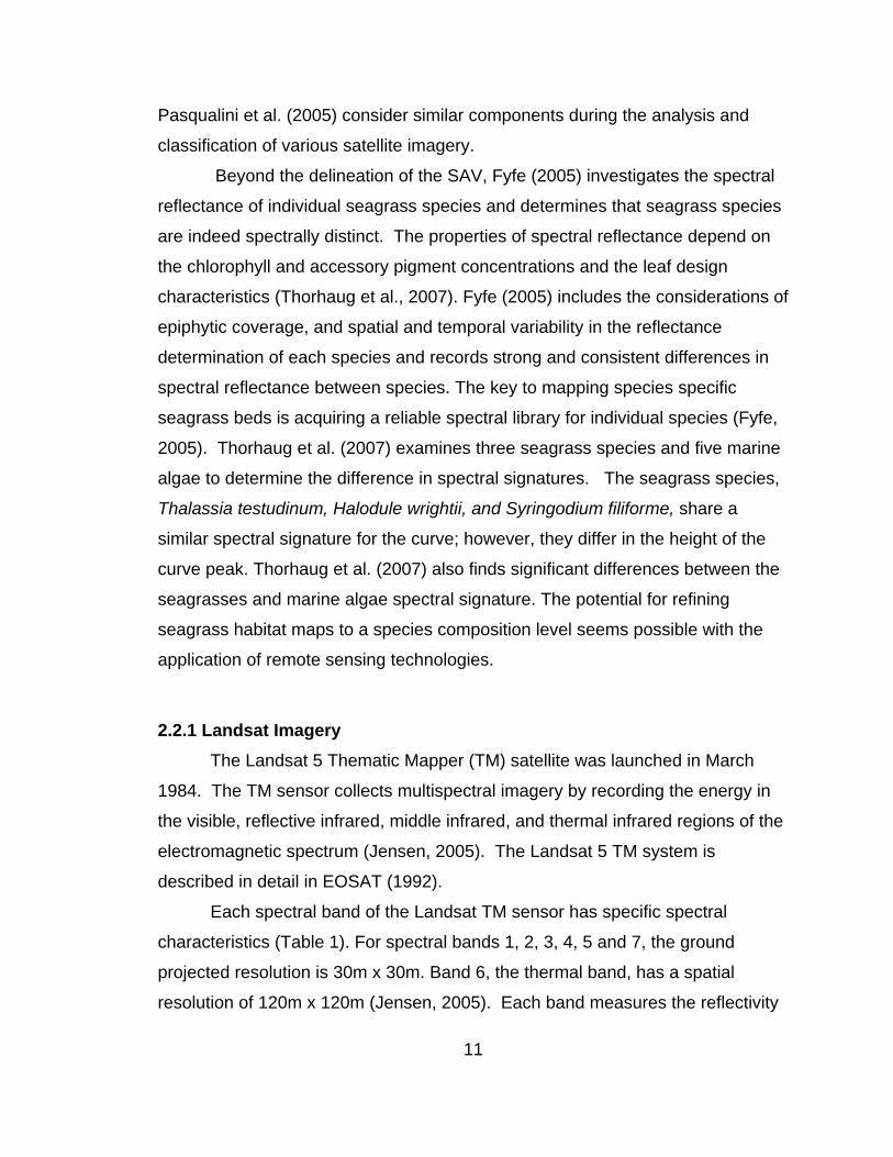
Pasqualini et al. (2005) consider similar components during the analysis and

classification of various satellite imagery.

Beyond the delineation of the SAV, Fyfe (2005) investigates the spectral

reflectance of individual seagrass species and determines that seagrass species

are indeed spectrally distinct. The properties of spectral reflectance depend on

the chlorophyll and accessory pigment concentrations and the leaf design

characteristics (Thorhaug et al., 2007). Fyfe (2005) includes the considerations of

epiphytic coverage, and spatial and temporal variability in the reflectance

determination of each species and records strong and consistent differences in

spectral reflectance between species. The key to mapping species specific

seagrass beds is acquiring a reliable spectral library for individual species (Fyfe,

2005). Thorhaug et al. (2007) examines three seagrass species and five marine

algae to determine the difference in spectral signatures. The seagrass species,

Thalassia testudinum, Halodule wrightii, and Syringodium filiforme, share a

similar spectral signature for the curve; however, they differ in the height of the

curve peak. Thorhaug et al. (2007) also finds significant differences between the

seagrasses and marine algae spectral signature. The potential for refining

seagrass habitat maps to a species composition level seems possible with the

application of remote sensing technologies.

2.2.1 Landsat Imagery

The Landsat 5 Thematic Mapper (TM) satellite was launched in March

1984. The TM sensor collects multispectral imagery by recording the energy in

the visible, reflective infrared, middle infrared, and thermal infrared regions of the

electromagnetic spectrum (Jensen, 2005). The Landsat 5 TM system is

described in detail in EOSAT (1992).

Each spectral band of the Landsat TM sensor has specific spectral

characteristics (Table 1). For spectral bands 1, 2, 3, 4, 5 and 7, the ground

projected resolution is 30m x 30m. Band 6, the thermal band, has a spatial

resolution of 120m x 120m (Jensen, 2005). Each band measures the reflectivity

12

at different wavelengths. Band 1, blue, measures 0.45-0.52 μm in the visible

spectrum. Due to the frequency of the wavelength, band 1 penetrates water.

Band 2, green, measures 0.52-0.60 μm in the visible spectrum. Studies suggest

that band 2 spans the region between the blue and red chlorophyll absorption

making it useful for the analysis of vegetation (Jensen, 2005). Band 3, red,

measures 0.63-0.69 μm in the visible spectrum and may be used for studies of

vegetation for the red chlorophyll absorption. Band 4 measures 0.76-0.90 μm in

the near-infrared spectrum. Band 4 is useful for the determination of biomass for

terrestrial vegetation, and the contrast of land and water. Band 5 measures 1.55-

1.75 μm in the mid-infrared spectrum, and is found useful for determining

turgidity and the amount of water in plants. Band 6 measures 10.40-12.50 μm in

the thermal spectrum related to the infrared radiant energy emitted from the

surface. Band 7 measures 2.08-2.35 μm in the mid-infrared spectrum. Band 7 is

mainly used for discriminating rock formations (Jensen, 2005).

Table 1. Landsat 5 TM band descriptions

Band Spectrum Resolution

(m) Spectral

Resolution (μm) Characteristics/Functions

1 blue 30x30 0.45-0.52 Penetration of water and

supports vegetation analysis

2 green 30x30 0.52-0.60 Reacts to the green

reflectance of vegetation

3 red 30x30 0.63-0.69 Reacts to the red chlorophyll

absorption and vegetation

4 near-infrared 30x30 0.76-0.90 Contrast of land and water, and terrestrial vegetation

5 mid-infrared 30x30 1.55-1.75 Useful for turgidity and

hydration in plants

6 thermal 120x120 10.40-12.50 Radiant thermal energy

7 mid-infrared 30x30 2.08-2.35 Determining rock formations

13

2.2.2 Aerial Photography Aerial photography is usually collected from a plane flying in concentric

transects over the study area. Depending on the altitude of the plane and the

camera specifications, the swath and resolution vary. Aerial photography also

requires preprocessing such as mosaicing the frames together and

georeferencing the imagery prior to spatial analysis (Kaufman, 2007).

Agencies use aerial photography to map the land surface characteristics

and shallow aquatic habitats including SAV. Aerial photography is collected in

analog or digital format. The historic aerial imagery is limited to black and white

or color film. The more current aerial photography is collected in a digital format.

The digital imagery usually focuses on the three visible spectral bands: red,

green, and blue, and may also include the near-infrared band (Kaufman, 2007).

True color photography uses the three visible bands only. Features of interest

are extracted from the images by a photointerpreter and used to produce maps.

2.3 Remote Sensing Classification 2.3.1 Imagery Classification

The extraction of thematic information from remote sensing data requires

a series of processing methods including preprocessing, selecting appropriate

logics and algorithms, and assessing the accuracy of the resultant product. The

preprocessing steps include radiometric and geometric correction (Jensen,

2005).

The classification of thematic information requires a defined logic and

algorithm appropriate for the data. The image classification method includes

parametric, nonparametric, or nonmetric logics. Parametric logic assumes that

the sample data belongs to a normally distributed population and knowledge of

the underlying density function (Jensen, 2005). The nonparametric logic allows

for sample data not from a normally distributed population. The nonmetric logic

may incorporate both ordinal and nominal scaled data in the classification

method. The algorithms may apply supervised or unsupervised methods. The

14

supervised classifications use known information extracted from training areas

concerning the image to label a specific class for every pixel in the image. The

unsupervised method allows the algorithm to differentiate between spectrally

significant classes automatically. A combination of the supervised and

unsupervised methods results in a hybrid approach.

2.3.2 Hard Classification Methods Two supervised parametric methods, also considered hard classification,

include the MLC and MDC algorithms. The MLC algorithm is a parametric

supervised method. Based on the statistical probability of a pixel value belonging

to a normally distributed population, the algorithm assigns the pixel to the most

likely class. The method assumes that the training data for each class in each

band are normally distributed (Jensen, 2005). Calculating the probability for the

density functions, the MLC algorithm assesses the variance of each training

class associated with the pixel brightness values. The MLC method is not

recommended for bimodal or n-modal distributions. Variations of the maximum

likelihood method without probability information assume that each class occurs

equally across the landscape of the image. The MDC algorithm is a direction

sensitive distance classification similar to the MLC method. The classification

method is based on the analysis of correlation patterns between variables and is

a useful way of determining similarity of an unknown pixel to a known one. The

MDC assumes that the covariances for all the classes are equal (Richards,

1999). Based on the distance threshold, the algorithm fits pixels to the nearest

class.

The unsupervised classification method used in this study is the Iterative

Self-Organizing Data Analysis Technique (ISODATA) (Jensen, 2005). The

ISODATA requires little input from the analyst. The ISODATA is based on the k-

means clustering algorithm. The clustering method uses multiple iterations to

determine the data grouping (Jensen, 2005). The cluster means are analyzed

and pixels are allocated to the most appropriate cluster. ISODATA is used to for

the initial examination of data to investigate the number of significant classes.

15

2.3.3 Soft Classification Methods

Two supervised nonparametric classification methods, also considered

soft classification, include linear spectral unmixing (LSU) and artificial neural

network (ANN) algorithms. Theoretically, the pixel-based seagrass abundance is

determined by examining the significant spectral signatures of seagrass in

individual pixels in the image with a LSU model. The LSU assumes that the

spectral signature is the linear sum of the set of pure endmembers which are

then weighted by their relative abundance (Hedley and Mumby, 2003).

According to Hedley and Mumby (2003) the application of LSU to the aquatic

environment is insufficient due to the light attenuation properties of the water

causing the divergence from the linear model. However, if a depth correction can

be applied to the pixels, then the LSU may produce reasonable results (Hedley

and Mumby, 2003).

The ANN is a layered feed-forward classification technique that uses

standard back-propagation for supervised learning. Researchers select the

number of hidden layers to use and choose between a logistic or hyperbolic

activation function. Learning occurs by adjusting the weights in the node to

minimize the difference between the output node activation and the output. One

layer between the input and output layers is usually sufficient for most learning

purposes (Pu et al., 2008). The learning procedure is controlled by a learning

rate, a momentum coefficient, and a number of nodes in the hidden layer that

need to be specified empirically based on the results of a limited number of tests.

The network training is done by repeatedly presenting training samples (pixels)

with known seagrass abundance. Network training is terminated when the

network output meets a minimum error criterion or optimal test accuracy is

achieved. Finally, the trained network can then be used to unmix each mixed

pixel. Therefore, ANN classification performs a non-linear classification and

spectral unmixing analysis.

16

Chapter 3

Methodology 3.1 Methodology Overview

The remote sensing analysis for the study follows the "Remote Sensing

Process" as described by Jensen (2005). This substantial process consists of

image preprocessing, image enhancement, and thematic information extraction

aiming to map the seagrass resources. The methodology for analysis of remote

sensing imagery follows an inductive logic approach. A deterministic empirical

model is applied to analyze the remote sensing data. This study applies

unsupervised and supervised classification methods to extract thematic

information from Landsat 5 TM imagery.

3.2 Data Sources Several types of data are readily available for St. Joseph Sound and

Clearwater Harbor. The remote sensing data available consists of aerial

photography, aerial photointerpretation maps, and Landsat 5 TM imagery.

The field survey data include information from the seagrass monitoring and

ambient water quality monitoring programs.

3.2.1 Remote Sensing Data Sources 3.2.1.1 Aerial Photointerpretation SAV Mapping

Available remote sensing data for the study area includes aerial

photographs and satellite imagery. The Southwest Florida Water Management

District (SWFWMD) collects high resolution natural color aerial photography

(SWFWMD, 2006). Collected on a 2-year cycle, the available digital imagery is

one-meter resolution.

17

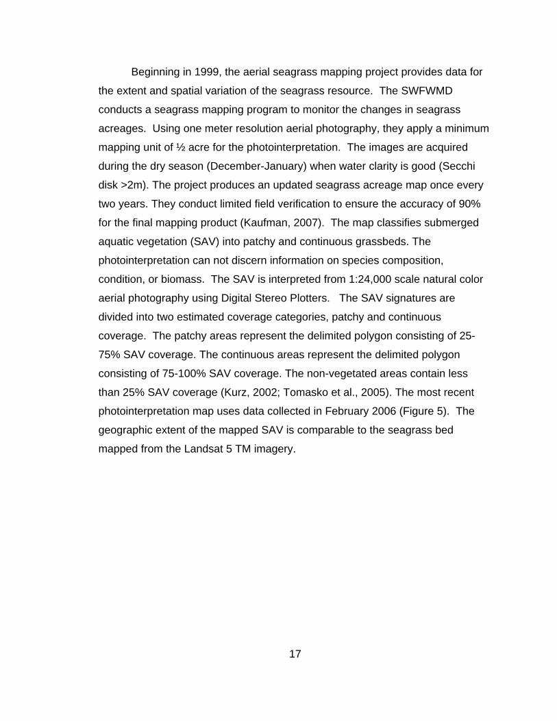
Beginning in 1999, the aerial seagrass mapping project provides data for

the extent and spatial variation of the seagrass resource. The SWFWMD

conducts a seagrass mapping program to monitor the changes in seagrass

acreages. Using one meter resolution aerial photography, they apply a minimum

mapping unit of ½ acre for the photointerpretation. The images are acquired

during the dry season (December-January) when water clarity is good (Secchi

disk >2m). The project produces an updated seagrass acreage map once every

two years. They conduct limited field verification to ensure the accuracy of 90%

for the final mapping product (Kaufman, 2007). The map classifies submerged

aquatic vegetation (SAV) into patchy and continuous grassbeds. The

photointerpretation can not discern information on species composition,

condition, or biomass. The SAV is interpreted from 1:24,000 scale natural color

aerial photography using Digital Stereo Plotters. The SAV signatures are

divided into two estimated coverage categories, patchy and continuous

coverage. The patchy areas represent the delimited polygon consisting of 25-

75% SAV coverage. The continuous areas represent the delimited polygon

consisting of 75-100% SAV coverage. The non-vegetated areas contain less

than 25% SAV coverage (Kurz, 2002; Tomasko et al., 2005). The most recent

photointerpretation map uses data collected in February 2006 (Figure 5). The

geographic extent of the mapped SAV is comparable to the seagrass bed

mapped from the Landsat 5 TM imagery.

18

Figure 5. Aerial Photointerpretation SAV Map based on 2006 aerial imagery (Kaufman, 2007).

19

3.2.1.2 Satellite Imagery The Landsat 5 Thematic Mapper (TM) imagery for this study was provided

by the Florida Center for Community Design and Research (FCCDR) at the

University of South Florida. The image was acquired on 2 May 2006 (Table 2).

The image was selected based on the low percentage of cloud cover and the

limited budget for the project. The spatial resolution of the Landsat 5 TM imagery

is 30m x 30m on the ground. The TM bands used in the study include 1 (blue), 2

(green), 3 (red), and 4 (near infrared). Bands 1, 2, and 3 were used for the

spectral signature of the SAV associated with water column. Band 4 was only

used for creation of masks.

The preprocessing steps for the image including geometric and

radiometric corrections were completed by the FCCDR prior to this study using

the ENVI Version 4.3 software program (ITT, 2006). The specifics of the

processes were presented by Andreu et al. (2008). The image was

georeferenced to the Universal Transverse Mercator map projection as

WGS1984 Zone 17N. The radiometric calibration used the Calibration tool to

convert the Landsat digital numbers to the at-sensor reflectance values (Andreu

et al., 2008). Andreu et al. (2008) performed the atmospheric correction by

subtracting the atmospheric path radiance estimated from pseudo-invariant dark

water locations.

Table 2. Landsat 5 TM image details.

Path/Row Acquisition Date Scene Identifier

17/41 May 2, 2006 5017041000612210

Processing System: Format: Product Type:

LPGS GeoTiff L5 TM SLC-off L1T Single Segmentation

20

Figure 6. Landsat 5 TM satellite image from May 2, 2006. The natural color composite was made via TM band 3, 2, 1 vs. Red, Green, and Blue.

21

3.2.2 Field Survey Data Available seagrass field survey data consists of information from the

Pinellas County Seagrass Monitoring Program (Meyer and Levy, 2008) and the

Pinellas County Ambient Water Quality Monitoring Program (Levy et al., 2008)

3.2.2.1 Seagrass Monitoring Data

The Pinellas County Seagrass Monitoring Program collects information on

the status of the seagrass resource. Data parameters include SAV species,

shoot density, canopy height, epibiont density, sediment type, and depth

information. Data points are collected using a 0.5-meter square quadrat. The

sampling occurs at the end of the growing season (Oct-Nov). The current

seagrass survey sampling design (2006-2008) consists of a combination of

stratified-random and permanent transects. The permanent transects intersect

the historical permanent transect sites. The random transects are spatially

stratified allocating sampling effort to the continuous and patchy grassbeds as

delineated from the seagrass aerial mapping project by the Southwest Florida

Water Management District (SWFWMD). In the study area, researchers sampled

42 sites in 2006 and 55 sites in 2007 (Figure 7). To account for variation and

inaccuracy in the seagrass mapping, 15% of the sampling effort is allocated to

areas that are not classified as patchy or continuous seagrass beds. The

transects are 30 m in length and placed parallel to the shoreline. Samplers

collect seven data points along each transect at 5 meter increments (Meyer and

Levy, 2008). The mean abundance and density of seagrass was calculated for

each transect from the seven observations. These means were used in the

development of the training data for the thematic data extraction from the remote

sensing imagery.

22

Figure 7. Pinellas County seagrass monitoring program results for Clearwater Harbor and St. Joseph Sound (Meyer and Levy, 2008).

23

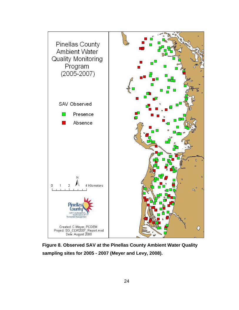
3.2.2.2 Water Quality Monitoring Data The Pinellas County Ambient Water Quality Monitoring Program collects

water quality and habitat information. The program samples 72 stratified random

sites per year in the study area. Developed in conjunction with Janicki

Environmental, Inc, the stratified-random design is based on a probabilistic

sampling scheme used by the Environmental Protection Agency (EPA) in their

Environmental Monitoring Assessment Program (EMAP) (Levy et al., 2008). The

EMAP-based design consists of overlaying a hexagonal grid by strata, and

randomly selecting a sample location within each grid cell. The stratified-random

design allows for statistical methods to be applied estimating population means

and confidence limits for water quality metrics (Janicki, 2003).

Habitat information collected at each site includes the presence/absence

of SAV, SAV species, and sediment composition. This study only uses the

2005 - 2007 data to coincide with the satellite imagery and seagrass information

(Figure 8).

24

Figure 8. Observed SAV at the Pinellas County Ambient Water Quality sampling sites for 2005 - 2007 (Meyer and Levy, 2008).

25

3.3 Landsat 5 TM Imagery Analysis Remote sensing information extraction techniques are used to estimate

the geographic extent and estimated coverage of the seagrass resource in the

study area. The goal of the analyses is to determine the feasibility of applying

satellite imagery interpretation to delineate the seagrass resource. The following

section describes the classification methods applied to the Landsat 5 TM

imagery.

3.3.1 Imagery Preprocessing The remote sensing data for the classification maps are based on a digital

Landsat 5 TM image. The study uses data consisting of field survey

measurements and ancillary datasets to develop training, testing, and validation

data subsets. The field measurements serve as the ground truth data for the

model validation as well as biomass and health information for the seagrass.

Although this study did not conduct laboratory analyses data, results adapted

from the studies of Fyfe (2005), and Thorhaug et al. (2007) provide spectral

reflectance information for the Florida seagrass ecosystem. Additional ancillary

data for the analysis includes maps from the Aerial Photointerpretation (AP)

Seagrass Mapping Project produced by the SWFWMD.

The thematic information extraction from the satellite imagery requires

several processing steps. The preprocessing includes radiometric, geometric

and topographic corrections, image enhancement, and initial image clustering

analysis. The radiometric and geometric corrections were completed for the

Landsat 5 TM imagery prior to this study by the FCCDR (Andreu et al., 2008).

The image processing is accomplished using the ENVI Version 4.3 software

program (ITT, 2006). The first processing step saves the raster files for bands 1,

2, 3, 4, 5, 6, and 7 into a single ENVI image. The image is then clipped to the

rectangular boundary of the study area (Figure 9). The clipped image consists of

400 columns and 1050 rows. Due to the strong spectral contrast between the

land based features and water, the open water area is masked from the image

26

using the near-infrared band 4 (Figure 10). The frequency distribution of the

pixels of the image (i.e., histogram technique) allows the segregation of the

image based on a threshold for the water versus land spectral properties. This

technique does not exclude all of the tidal flat areas in the study area.

Figure 9. Landsat 5 TM imagery clipped to the study area from 2 May 2006

27

Figure 10. Mask delineated from band 4 (near infrared).

3.3.2 Imagery Classification

To initially investigate the spectral classes of the image the Equalization

image enhancement is applied to bands 1, 2, and 3 (Figure 11). An image

clustering analysis is conducted using an unsupervised classification (ISODATA)

prior to the supervised classification. The ISODATA classification method is

applied to bands 1-3 and categorized the data into 10 subclasses. The resultant

28

classification is visually compared to the field survey information to detect spatial

correlations and estimated accuracy. The classes are merged into three

categories and an environmentally relevant label was applied. The classes are

land, SAV, and No SAV.

Figure 11. Landsat 5 TM image enhancement using Equalization function.

29

To map the seagrass resource from the TM imagery, two parametric

supervised classifications, Maximum Likelihood classification (MLC) and

Mahalanobis Distance classification (MDC), are performed on the Landsat 5 TM

imagery. The first three bands of the Landsat 5 TM imagery are used for these

classification methods. These bands have centered wavelengths of 485 nm, 560

nm, and 660 nm, respectively. The supervised image classifications use field

survey seagrass information for the training signature, as well as, testing and

validation. The classifications are conducted with two levels of SAV delineation.

The first analysis focuses on the presence versus absence of SAV. The training

and testing data categories for this classification include absence (<25% SAV)

and presence (25-100% SAV). The second analysis uses three classification

categories to delineate the estimated coverage of the SAV. The training and

testing data categories include No SAV (<25% SAV), Patchy (25-75% SAV), and

Continuous (75-100% SAV). Regions of interest (ROIs), delineated from the TM

imagery for the training and testing areas, are interpreted from a combination of

the Pinellas County Seagrass Monitoring field survey data and 6-inch resolution

aerial photography. The selected grid cells are merged and imported into the

ENVI 4.3 software as ROIs (ITT, 2006). Each ROI consists of 12 polygons with

a minimum of 50 pixels in each polygon. The ROIs are selected from the areas

homogeneous with spatial and spectral properties. The ROIs cover a range of

water depths, and are spatially distributed throughout the study area. The

estimated percent coverage for SAV is based on the mean abundance of

seagrass calculated for each field survey sampling location. Using ArcMap 9.2

software, a 30 m x 30 m grid is created to coincide with the seagrass field survey

data (ESRI, 2006). The aerial photography is used to compare the grid cells

surrounding the field survey transect to ensure a homogeneous area for the ROI

polygon.

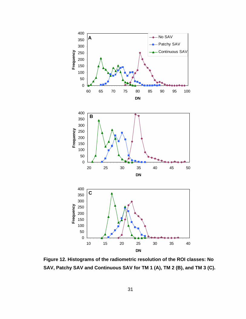
The spectral properties of the ROIs determine the feasibility of delineating

the classes in the classification map. By calculating the radiometric resolution

30

digital number (DN) for the ROIs in each spectral band, the separability of the

classes is determined. Descriptive statistics are calculated for the ROI training

data (Table 3). The separability of the ROI categories is examined for the three

spectral bands (Figure 12). The ability to accurate separate the categories is

relative to the overlap of the histogram curves. As the overlap of the histogram

curves increases, the categories become more difficult to separate. The patchy

and continuous SAV categories are expected to overlap. In the histograms for

band 1 and band 2, there is limited overlap between the No SAV and SAV

classes. The separability between the SAV and No SAV categories is greatest

for band 2. The categories have the least separability between categories in

band 3. This analysis suggests that it is feasible to delineate the SAV and No

SAV classes using the visible bands. The overlap between the Patchy and

Continuous SAV classes may limit the ability to accurately delineate them during

classification. Table 3. Radiometric Resolution descriptive statistics calculated for the ROI training data.

ROI class Pixels BandMinimum

DN Maximum

DN Mean DN

Standard Deviation

No SAV 1401 1 75 99 82.51 3.12 2 31 49 35.22 2.17 3 19 37 23.68 2.09 Patchy SAV 1154 1 65 89 73.85 3.51 2 24 37 29.00 1.89 3 16 27 21.48 2.15 Continuous SAV 1493 1 60 79 68.25 3.65 2 21 33 25.40 2.15 3 14 27 18.62 2.04

31

A

0

50100

150200

250

300350

400

60 65 70 75 80 85 90 95 100

DN

Freq

uenc

y

No SAV

Patchy SAV

Continuous SAV

B

050

100150200250300350400

20 25 30 35 40 45 50

DN

Freq

uenc

y

C

050

100150200250300350400

10 15 20 25 30 35 40

DN

Freq

uenc

y

Figure 12. Histograms of the radiometric resolution of the ROI classes: No SAV, Patchy SAV and Continuous SAV for TM 1 (A), TM 2 (B), and TM 3 (C).

32

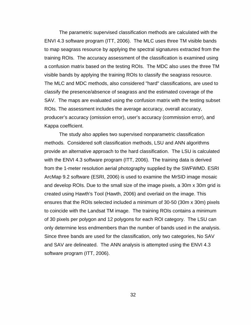
The parametric supervised classification methods are calculated with the

ENVI 4.3 software program (ITT, 2006). The MLC uses three TM visible bands

to map seagrass resource by applying the spectral signatures extracted from the

training ROIs. The accuracy assessment of the classification is examined using

a confusion matrix based on the testing ROIs. The MDC also uses the three TM

visible bands by applying the training ROIs to classify the seagrass resource.

The MLC and MDC methods, also considered "hard" classifications, are used to

classify the presence/absence of seagrass and the estimated coverage of the

SAV. The maps are evaluated using the confusion matrix with the testing subset

ROIs. The assessment includes the average accuracy, overall accuracy,

producer’s accuracy (omission error), user’s accuracy (commission error), and

Kappa coefficient.

The study also applies two supervised nonparametric classification

methods. Considered soft classification methods, LSU and ANN algorithms

provide an alternative approach to the hard classification. The LSU is calculated

with the ENVI 4.3 software program (ITT, 2006). The training data is derived

from the 1-meter resolution aerial photography supplied by the SWFWMD. ESRI

ArcMap 9.2 software (ESRI, 2006) is used to examine the MrSID image mosaic

and develop ROIs. Due to the small size of the image pixels, a 30m x 30m grid is

created using Hawth's Tool (Hawth, 2006) and overlaid on the image. This

ensures that the ROIs selected included a minimum of 30-50 (30m x 30m) pixels

to coincide with the Landsat TM image. The training ROIs contains a minimum

of 30 pixels per polygon and 12 polygons for each ROI category. The LSU can

only determine less endmembers than the number of bands used in the analysis.

Since three bands are used for the classification, only two categories, No SAV

and SAV are delineated. The ANN analysis is attempted using the ENVI 4.3

software program (ITT, 2006).

33

3.3.3 Classification Accuracy Analysis Post-processing includes several steps to ensure the accuracy of the

classification map. The validation of the classification requires a data source

independent from the training and testing data. The validation ROIs for this study

are determined from the seagrass data collected by the Pinellas County Ambient

Water Quality Monitoring Program. The validation accuracy assessment is

calculated using the ESRI ArcMap 9.2 software program (ESRI, 2006). The

classification images are exported from the ENVI 4.3 software as ESRI grid files

and clipped to the extent of the study area using ESRI Spatial Analyst Extension

(ESRI, 2006). The validation data includes spatial and temporal information on

the presence/absence and species composition of SAV. Due to the sampling

methods, the validation data point location accuracy has a radius of 10 m.

Hawth’s Analysis Tool (Hawth, 2006) is used in ESRI ArcMap 9.2 (ESRI, 2006)

to analyze the correlation between the validation data and the classification map.

Using the Intersect Point function in Hawth’s Tools, the vector validation points

and the raster classification map are processed. The correlation matrix is

developed to assess the accuracy of the classification.

3.4 Analyses The comparison of the classification maps is necessary to assess the

most appropriate method for SAV delineation. The estimated accuracy from the

validation analysis and spatial variation is used to compare the classification

maps. The validation estimated accuracies are compared using descriptive

statistics calculated with Microsoft Excel. The spatial comparison is described in

the following section.

3.4.1 Comparison to existing maps The AP mapping project conducted by the SWFWMD provides an

estimate of the SAV acreage for the study area. Although the project aims for

90% accuracy for the ground-truth points, the geographic extent of the study

restricts the validation to approximately 10 sites within Clearwater Harbor and St.

34

Joseph Sound. To estimate the accuracy of the AP maps, the validation data

from the Pinellas County Ambient Water Quality Monitoring Program is used to

develop a correlation matrix. The Intersect Point Function in Hawth’s Analysis

Tool (Hawth, 2006) is used in ESRI ArcMap 9.2 (ESRI, 2006) to analyze the

correlation between the validation data and the AP map.

The Landsat 5 TM classification maps developed in this study are

compared to the results from the AP mapping project conducted by the

SWFWMD. To investigate the variation between the mapping products, a spatial

correlation is completed using the ESRI ArcMap 9.2 software program with the

Spatial Analyst Extension. The total area is calculated for the classes of SAV,

and No SAV. The areas are compared between the two classification methods.

The classification maps are converted into raster grids with 30 m pixel cell

dimensions. The grids are overlaid and a comparison analysis is conducted using

the Raster Calculator (ESRI, 2006). The difference in SAV acreage is evaluated

to determine the effectiveness of the remote sensing supervised classification

methods in comparison to the AP mapping project.

3.4.2 Ability to Map SAV variation The classification methods are analyzed to assess the minimum amount

of variation that may be detected by the classification. The ability to assess the

variation is based on the accuracy of the classification method as determined by

the testing ROI confusion matrix and the validation assessment. The detectable

variation in the SAV is related to overall accuracy of the classification. The ESRI

ArcMap 9.2 software program is used to calculate the areas for each class

(ESRI, 2006).

35

Chapter 4

Results and Discussion

4.1 Classification Results The unsupervised and supervised methods produce classification maps

with various accuracies. The unsupervised classification method is similar in

validation accuracy to the supervised hard classification methods. The

supervised soft classification methods did not produce reasonable results.

Overall the supervised hard classifications are the most appropriate to map the

SAV in the study area.

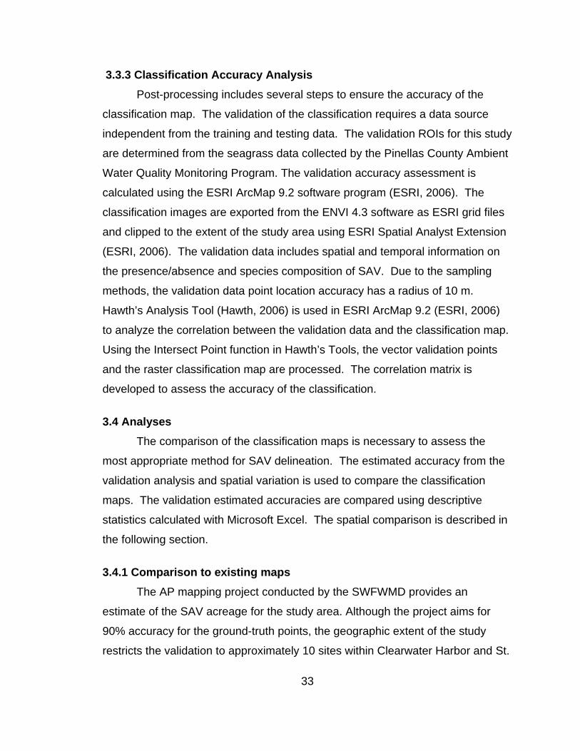
4.1.1 Unsupervised Classification The unsupervised ISODATA classification interprets seven categories

from the Landsat 5 TM image. The categories are merged into two classes and

labeled with environmentally relevant descriptions, SAV and No SAV. The

ISODATA classification map (Figure 13) displays the spatial extent of the SAV in

the study area. The ISODATA classification reasonably delineates the spectral

classes for the SAV features. A validation assessment is conducted using an

independent data set from the Pinellas County Ambient Water Quality Monitoring

Program (Levy et al, 2008). This point data provides information on the

presence/absence and species composition of the SAV. The validation dataset

(n=216) is compared to the class of the coinciding pixel. The ISODATA

validation estimates 76% accuracy for correctly classifying the SAV and 51% for

No SAV with an overall accuracy estimate of 68% (Table 6).

36

Figure 13. Unsupervised ISODATA classification of Landsat 5 TM image with environmentally relevant labels.

37

4.1.2 Supervised Classification 4.1.2.1 Hard Classification

The supervised parametric classification methods, Maximum Likelihood

(MLC) and Mahalanobis Distance (MDC), uses ROIs developed from the field

survey data to delineate the spectral signatures of the SAV. The methods are

first used to delineate the presence/absence of SAV. Then, the methods are

applied to delineate the estimated coverage of the SAV. Of these applications,

the hard classification methods have a higher overall accuracy for separating the

presence/absence of SAV.

4.1.2.1.1 Presence/Absence of SAV

Both the MLC and MDC (Figure 14) depict reasonable maps of the

presence/absence of SAV. Calculated with a confusion matrix using the testing

ROIs, the overall accuracy of the MLC is 85.54 % with a Kappa coefficient of

0.69 (Table 4). The overall accuracy of the MDC is 86.79% with a Kappa

coefficient of 0.70. Both classifications produce similar accuracies. The

producer’s accuracy is slightly better for the classification of SAV in the MDC

(Table 5), and for the classification of the No SAV in the MLC. The user’s

accuracy is slightly better for the classification of SAV in the MLC (Table 5), and

for the classification of the No SAV in the MDC.

In addition to the accuracy assessment for the classification maps, a

validation assessment is conducted using an independent data set from the

Pinellas County Ambient Water Quality Monitoring Program (Levy et al, 2008).

This point data provides information on the presence/absence and species

composition of the SAV. The validation dataset (n=216) is compared to the class

of the corresponding pixel. The MLC validation estimates 66% accuracy for

correctly classifying the SAV and 69% for No SAV with an overall accuracy

estimate of 67% (Table 6). The MDC validation estimates 74% accuracy for

correctly classifying the SAV and 58% for No SAV with an overall accuracy

estimate of 68% (Table 6).

38

Figure 14. Supervised classification of Landsat 5 TM image using the Mahalanobis Distance and Maximum Likelihood methods.

39

Table 4. Accuracy estimates for the supervised classification methods.

Overall

Accuracy (%) Kappa

Coefficient Maximum Likelihood 85.54 0.69 Mahalanobis Distance 86.79 0.70

Table 5. Supervised classification commission and omission errors, and producer and user’s accuracy.

Commission

(%) Omission

(%) Commission

(Pixels) Omission (Pixels)

Producer Accuracy

User Accuracy

Maximum Likelihood SAV 7.77 14.85 214/2754 443/2983 85.15 92.23 No SAV 24.73 13.70 443/1791 214/1562 86.15 75.27 Mahalanobis Distance SAV 9.26 11.03 271/2925 329/2983 88.97 90.74 No SAV 20.31 17.35 329/1620 271/1562 82.65 79.69 Table 6. Validation for classification methods SAV presence/absence

SAV Accuracy %

No SAV Accuracy %

Overall Accuracy %

ISODATA 76.6 51.8 68.4 Maximum Likelihood 66.2 69.4 67.3 Mahalanobis Distance 74.2 58.5 68.9

A comparison of the MLC and MDC maps presents discrepancies in the

classification of SAV in the intertidal areas. Figure 15 illustrates a shallow

seagrass bed that is often exposed at low tide. The MDC correctly classifies the

area as SAV; whereas, the MLC classifies the majority of the seagrass bed as

No SAV. Overall, the MLC and MDC produce very similar classification maps.

40

Figure 15. Differences (red circle) between the supervised classification of Landsat 5 TM image using the Mahalanobis Distance and Maximum Likelihood methods.

41

4.1.2.1.2 Estimated Coverage of SAV

Both the MLC and MDC (Figure 16) depict reasonable maps of the

estimated coverage of SAV. Calculated with a confusion matrix using the testing

ROIs, the overall accuracy of the MLC is 74 % with a Kappa coefficient of 0.61

(Table 7). The overall accuracy of the MDC is 65% with a Kappa coefficient of

0.47. The MLC produces better accuracies than MDC in the classification of the

estimated coverage of SAV for this case. The producer’s accuracy is better for

the classification of No SAV and the continuous and patchy SAV in the MLC

(Table 8). The user’s accuracy is better for the classification of continuous and

patchy SAV in the MLC (Table 8), and similar in both methods for the

classification of No SAV.

In addition to the accuracy assessment for the classification maps, a

validation assessment is conducted using an independent data set from the

Pinellas County Ambient Water Quality Monitoring Program (Levy et al, 2008).

This point data provides information on the presence/absence and species

composition of the SAV. Since the data only supports the comparison of SAV

and No SAV classes, the patchy and continuous classes of the MLC and MDC

are combined for the validation. The validation dataset (n=216) is compared to

the class of the corresponding pixel. The MLC validation estimates 86%

accuracy for correctly classifying the SAV and 37% for No SAV with an overall

accuracy estimate of 70% (Table 9). The MDC validation estimates 85%

accuracy for correctly classifying the SAV and 36% for No SAV with an overall

accuracy estimate of 69% (Table 9).

42

Figure 16. Supervised classification of Landsat 5 TM image using the Mahalanobis Distance and Maximum Likelihood methods.

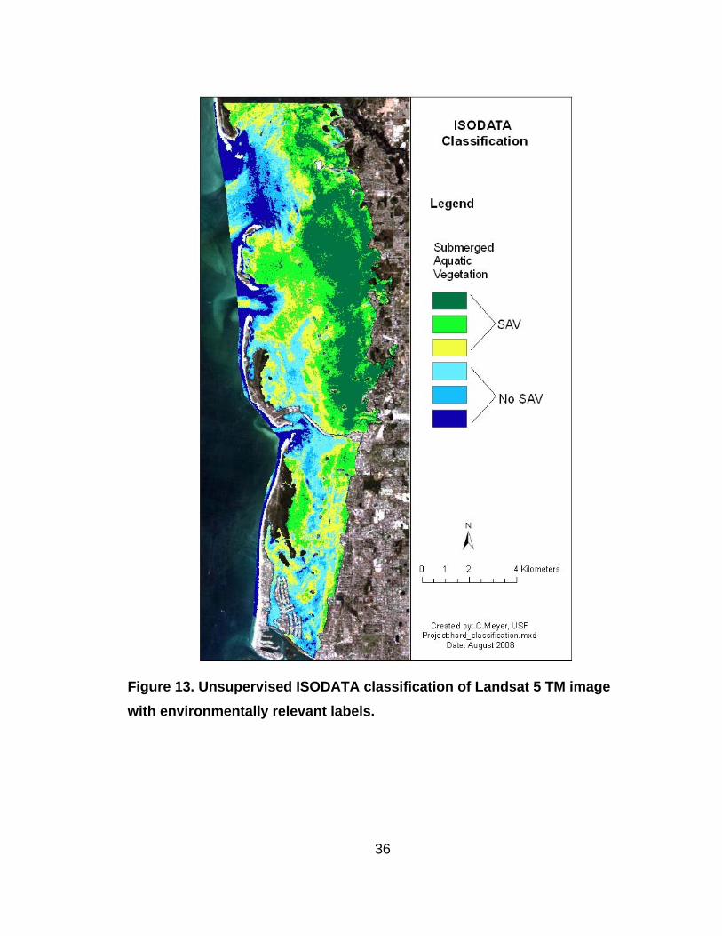
43

Table 7. Accuracy estimates for the supervised classification methods.

Overall

Accuracy (%) Kappa

Coefficient Maximum Likelihood 74 0.61 Mahalanobis Distance 65 0.47

Table 8. Supervised classification commission and omission errors, and producer and user’s accuracy.

Commission

(%) Omission

(%) Commission

(Pixels) Omission (Pixels)

Producer Accuracy

User Accuracy

Maximum Likelihood Continuous 25.93 18.85 202/779 134/711 81.15 74.07 Patchy 44.99 37.10 337/749 243/655 62.90 55.01 No SAV 5.53 22.48 41/741 203/903 77.52 94.47 Mahalanobis Distance Continuous 48.91 24.33 515/1053 173/711 75.67 51.09 Patchy 54.63 45.34 431/789 297/655 54.66 45.37 No SAV 5.89 34.57 64/1086 540/1562 65.43 94.11 Table 9. Validation for classification methods SAV estimated coverage

SAV

Accuracy % No SAV

Accuracy % Overall

Accuracy % Maximum Likelihood 86.5 37.8 70.2 Mahalanobis Distance 85.8 36.5 69.3

A comparison of the MLC and MDC maps presents discrepancies in the

classification of patchy versus continuous SAV main areas with deeper water.

Figure 17 illustrates a deep (>2m) seagrass bed. The MLC correctly classifies

the area as patchy SAV; whereas, the MDC classifies the majority of the

seagrass bed as continuous SAV. Figure 18 shows a deeper area classified as

mostly continuous SAV by the MDC and patchy SAV by the MLC. Unfortunately,

the field survey data does not have enough sampling sites in this area to discern

44

which classification is more accurate. Overall, the MLC and MDC produce

similar classification maps; however, the MLC is the most accurate and

reasonable of the two methods.

Figure 17. Differences (red circle) between the supervised classification of Landsat 5 TM image using the Mahalanobis Distance and Maximum Likelihood methods.

45

Figure 18. Differences (red rectangle) between the supervised classification of Landsat 5 TM image using the Mahalanobis Distance and Maximum Likelihood methods.

46

4.1.2.2 Soft Classification In an attempt to improve the results of the classification technique, the

study also applied two supervised nonparametric classification methods.

Considered soft classification methods, linear spectral unmixing and neural

network algorithms provide an alternative approach to the hard classification.

Contrary to the hypothesis the “soft” classification methods, LSU and ANN did

not improve the resolution and accuracy of the hard classification map.

However, the application of these methods may provide improved classifications

for imagery with more than three useful bands in the aquatic environment.

4.1.2.2.1 Artificial Neural Networks

The artificial neural network (ANN) classification does not produce

reasonable results (Figure 19). The ANN classifies less than 5% of the study

area as SAV. Although this method is not successful in this instance, the use of

a different software program or algorithm may provide more reasonable results.

In addition, these may be explained by the low spectral difference of between the

different classes or the number limitation of the spectral dimension of only three

visible bands.

47

Figure 19. Artificial Neural Network Classification of Landsat 5 TM image.

48

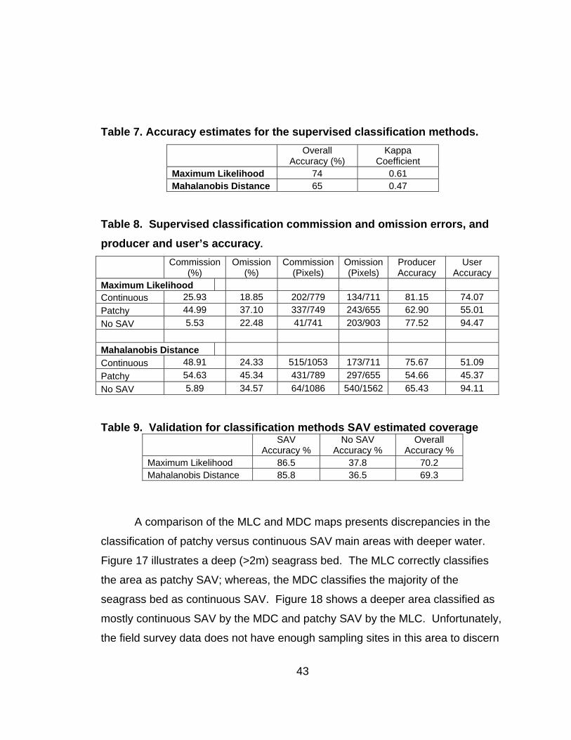
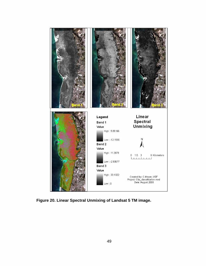
4.1.2.2.2 Linear Spectral Unmixing

The linear spectral unmixing (LSU) is also applied to the Landsat TM

image. The LSU does not produce reasonable results for the classification map

(Figure 20). The amount of endmember classes for the LSU must be less than

the number of spectral bands used for the classification. Since only three

spectral bands (1, 2, and 3) are appropriate for the classification of SAV, only two

endmember classes could be delineated.

49

Figure 20. Linear Spectral Unmixing of Landsat 5 TM image.

50

4.2 Assessment of Classification Methods The assessment of the classification methods compares the accuracy and

validation estimates, as well as, the spatial distribution of the variation. The aerial

photointerpretation (AP) map is used as a baseline for the comparison of the

MDC and MLC classifications. The ability of the classification methods to map

SAV is estimated from the accuracy and validation results for each technique.

4.2.1 Accuracy Comparison of SAV Maps

Prior to comparing AP map to the MLC classification map, an accuracy

assessment is completed for the AP map. Due to the limited ground truth data

collected with the AP project, the 90% accuracy can not be compared to the

products from this study. The validation method for the classification maps is

applied to the AP map. Since the validation dataset only supports the comparison

of SAV and No SAV classes, the patchy and continuous classes of the AP map

are combined for the validation. The validation dataset (n=216) is compared to

the classes of the corresponding pixels (Figure 21). The AP validation estimates

81% accuracy for correctly classifying the SAV and 51% for No SAV with an

overall accuracy estimate of 71% (Table 10).

51

Figure 21. Comparison of validation data to the SAV Aerial Photointerpretation Map, 2006.

52

The comparison of the classification methods relies on the validation

accuracy estimates since it was the only available qualifier for all the methods.

Although the overall estimated accuracy varies slightly between classification

methods, the estimated accuracy for the classes of SAV and No SAV varies

significantly (Figure 22). To examine the variation between the methods the

means and standard errors are calculated. For the six methods the SAV

estimated accuracy from the validation analysis is 78% for SAV (SE= 3.15), 50%

for No SAV (SE= 5.10), and 69% for Overall (SE= 0.58). The AP map has the

highest overall accuracy (71.4%). The MDC (69.3%) and MLC (70.2%) maintain

a close overall accuracy; however, the accuracy associated with mapping No

SAV is below 40%. Although the overall accuracy for the MLC and MDC is lower

for the presence/absence than the estimated coverage classifications, the No

SAV accuracy is much higher. To consider the best classification method, the

researcher needs to determine the focus of the study and the omission and

commission statistics related to each method.

Table 10. Comparison of validation for classification methods

Classification Method SAV

Accuracy % No SAV

Accuracy % Overall

Accuracy % ISODATA 76.6 51.8 68.4 MLC (Presence/Absence) 66.2 69.4 67.3 MDC (Presence/Absence) 74.2 58.5 68.9 MLC (Estimated coverage) 86.5 37.8 70.2 MDC (Estimated coverage) 85.8 36.5 69.3 AP map 81.1 51.2 71.4

53

0

10

20

30

40

50

60

70

80

90

100

ISODATA

MLC (P

resen

ce/Abs

ence

)

MDC (Pres

ence

/Absen

ce)

MLC (E

stimate

d Cov

erage

)

MDL(Esti

mated C

overa

ge)

AP

Valid

atio

n A

ccur

acy

%

SAV No SAV Overall

Figure 22. Estimated classification accuracies derived from validation analysis for different classification methods.

4.2.2 Spatial Comparison to Existing SAV Maps The classification methods with the highest accuracy, kappa coefficient,

and validation accuracy are compared to the existing AP map to determine

spatial variation. For the delineation of presence/absence of SAV, the MDC has

86% overall accuracy with a 0.70 Kappa coefficient calculated from the testing

ROIs. The overall validation accuracy for the MDL is 68%. For the delineation of

SAV estimated coverage, the MLC has 74% overall accuracy with a 0.61 Kappa

coefficient calculated from the testing ROIs. The overall validation accuracy for

the MLC is 70%. The AP map has an overall validation accuracy of 71%

calculated for this study. For each classification method the area per class is

54

calculated (Table 11). The greatest difference is between the delineation of the

SAV (patchy) class in the MLC (48.76 km2) and the AP (11.50 km2).

Table 11. Area calculated for each classification method.

Number of Pixels km2 MDC (Presence/Absence) No SAV 67277 60.55 SAV 80623 72.56 Land 29000 26.10 MLC (Estimated coverage) No SAV 46049 41.44 SAV (patchy) 54183 48.76 SAV (continuous) 47668 42.90 Land 29000 26.10 AP (Estimated coverage) No SAV 44413 39.97 SAV (patchy) 12782 11.50 SAV (continuous) 49250 44.33 Land 14248 12.82

The spatial comparison of these classifications displays areas of variation

between the maps. The comparison of the AP and MDC for the

presence/absence of SAV shows most discrepancies in the deep water areas

along the edge of the seagrass bed (Figure 23). The classes of Land and No

SAV are combined to focus on the similarity for the SAV classification. The AP

and MDC both map 43.70 km2 of SAV with a discrepancy of 18.74 km2 which is

16% of the study area (Table 12). The comparison of the AP and MLC for the

SAV estimated coverage displays the most discrepancies in the deep water

areas and along the edges of the seagrass beds (Figure 24). The AP and MLC

map 32.79 km2 of SAV at the same estimated coverage class, and 16.30 km2 of

SAV with differing estimated coverage classes. The discrepancies cover 21.19

km2 which represents 19% of the study area (Table 13).

55

The spatial variation in the classification may be affected by the water

increased water depth along the edges of the seagrass beds. The AP is known to

be limited to approximately 2 m water depth due to the refraction and absorption

of the penetrating light wavelengths. The areas with dredged boat channels are

consistently misclassified by the MDC and MLC. The width of the boat channels

in comparison to the pixel size of the Landsat 5 TM imagery may indicate that the

feature is too small to be accurately mapped by these classification methods and

resolution. Other areas of discrepancy include the intertidal seagrass beds.

Depending on the tidal stage at the acquisition time of the Landsat TM imagery,

some of the seagrass beds may be exposed with little or no water separating the

seagrass blades from the air. This may cause a variation in the spectral

signature of the seagrass.

56

Table 12. Aerial Photointerpretation versus Mahalanobis Distance Classification

Number of pixels km2 Discrepancy 20825 18.74 Land/No SAV 51059 45.95 SAV 48560 43.70

Figure 23. Discrepancies between the AP and MDC for the presence/absence of SAV.

57

Table 13. Aerial Photointerpretation versus Maximum Likelihood Classification

Number of pixels km2 Discrepancy 23547 21.19 Land/No SAV 42339 38.10 SAV (same estimated coverage) 36442 32.79 SAV (different estimated coverage) 18116 16.30

Figure 24. Discrepancies between the AP and MLC for the estimated coverage of SAV.

58

4.2.3 Ability to Map SAV Variation The ability to map the seagrass resource is essential to the management

and protection of the resource. The remote sensing methods used to map and

estimate the coverage of seagrass must provide reliable information. The

detectable amount of the seagrass resource is related to the accuracy of the

classification method. To determine the limitations of mapping seagrass, the

MDC (presence/absence of SAV) and the MLC (estimated coverage of SAV)

classifications were analyzed. Additionally, the AP classification was examined

for the ability and confidence of mapping seagrass resource.

Based on the calculated accuracies from the confusion matrix analysis,

the potential variation for misclassification ranges from 10.86 km2 - 41.39 km2

(Table 14). Based on the calculated accuracies from the validation analysis, the

potential variation for the misclassification ranges from 31.06 km2 - 49.51 km2.

These potential variation estimates are based on the entire study area and not

solely on the seagrass resource.

Table 14. Potential variation associated with the estimated accuracies for the classification methods.

Accuracy %

Potential Variation (Number

of Pixels)

Potential Variation

(km2) MDC (Presence/Absence) Overall Accuracy 86.79 23368 21.03 Validation Accuracy 68.9 55016 49.51 MLC (Estimated coverage) Overall Accuracy 74 45991 41.39 Validation Accuracy 70.2 52713 47.44 AP (Estimated coverage) Overall Accuracy 90 12069 10.86 Validation Accuracy 71.4 34517 31.06

59

The potential to map and assess the variation in the seagrass is important

to the development of resource management plans. The AP mapping project

currently assesses the change in the resource. The estimated change in the

seagrass resource between 2004 and 2006 was 2.92% increase (Kaufman,

2007). According to the analysis in this study, the 1.63 km2 increase in seagrass

is below the detectable change threshold. Therefore, the resource is most likely

within the variance of the classification method rather than truly increasing.

Caution should be used when formulating conclusions on the fine scale trends

associated with the classification maps.

60

Chapter 5

Conclusions

The application of remote sensing techniques to map the seagrass

resource has been examined in many studies in the past two decades with

varying success. The challenges of delineating habitat classes in the aquatic

environment affect the accuracy and reliability of the produced maps. The

prominent method of seagrass mapping in Florida, U.S.A. is the AP mapping

method. According to the results from this study, the accuracy of the ranges

from the estimated validation accuracy of 71.4% to the project's assessed

accuracy of 90%. The AP study provides a consistent baseline for the detection

of spatial change in the seagrass resource. However, due to the temporal scale

of the AP project, a 2-year cycle, the produced maps may not detect shorter

temporal variation in the seagrass resource. The occurrence of natural and

anthropogenic events may cause damage to the seagrass resource that would

not be detected for up to 2 years. To quickly assess the damage to the resource

following the occurrence of a natural or anthropogenic disturbance, such as

hurricanes or oil spills, the environmental resource managers require a reliable

tool to assess the spatial extent of the seagrass resource on a finer temporal

scale. The temporal availability of the Landsat 5 TM imagery, 16-20 days,

provides a suitable option to detect and assess damage to the seagrass

resource.

This study provides an overview of thematic information extraction

methods applied to the classification of the seagrass resource. The results

suggest that the ISODATA and MDC methods provide the most reliable maps

delineating the presence/absence of SAV. For the delineation of SAV estimated

coverage maps, the MLC method is the most appropriate technique according to

61

this study. While these remote sensing methods provide classification maps with

similar accuracies to the AP method, additional research is necessary to improve

and evaluate the classification techniques.

To improve the accuracy for these remote sensing techniques, additional

studies may focus on the refinement of the spectral signatures of the seagrass

habitats. Future studies using the Landsat 5 TM imagery may apply a spectral

library for the SAV species in the study area. The time series of the Landsat 5

TM imagery beginning in 1984 may provide an opportunity to apply the

classification methods from this study to the historical Landsat Imagery in an

attempt to assess the temporal change over the past two decades. Information

regarding the spatial and temporal change dynamics assists environmental

resource managers in the development of successful management and

protection plans for the seagrass resource.

In conclusion, the results of this study suggest that the application of

remote sensing methods is appropriate to assess the spatial extent of the

seagrass resource in Clearwater Harbor and St. Joseph Sound, Florida. The

supervised classification methods applied to the Landsat 5 TM imagery provide

reasonable results that were comparable to the existing AP classification

methods. While there is always opportunity for improvement, this study offers

the option of using satellite imagery as a reliable data source for the mapping of

the seagrass resource.

62

References Cited (2006) Coastal Remote Sensing Toolkit. Coastal CRC and Centre for

Remote Sensing and Spatial Information Science, The University of Queensland. http://www.gpa.uq.edu.au/CRSSIS/tools/rstoolkit/

Andreu, Michael G., Melissa H. Friedman, Shawn M. Landry and Robert J. Northrop. 2008. City of Tampa Urban Ecological Analysis 2006-2007. Final Report to the City of Tampa, April 24, 2008. City of Tampa, Florida. Andrefouet, S., Kramer, P., Torres-Pulliza, D., Joyce, K. E., Hochberg, E. J.,

Garza-Perez, R., Mumby, P. J., Riegl, B., Yamano, H., White, W. H., Zubia, M., Brock, J. C., Phinn, S. R., Naseer, A., Hatcher, B. G., and Muller-Karger, F. E. 2003. Multi-site evaluation of IKONOS data for classification of tropical coral reef environments. Remote Sensing of Environment 88:128-143.

Avery, W.M. and Johansson, J.O.R. 2001. Tampa Bay Interagency Seagrass

Monitoring Program: Seagrass species distribution and coverage along fixed transects 1997-2000. Tampa: Tampa Bay National Estuary Program.

Brooks, R. A. and Bell, S.S. 2001. Mobile corridors in marine landscapes:

enhancement of faunal exchange at seagrass/sand ecotones. Journal of Experimental Marine Biology and Ecology 264:67-84.

Chauvaud, S., Bouchon, C., and Manieres, R. 1998. Remote sensing

techniques adapted to high resolution mapping of tropical coastal marine ecosystems (coral reefs, seagrass beds, and mangrove). International Journal of Remote Sensing 19(18): 3625-3639.

Dawes, C.J., Phillips, R.C., and Morrison, G. 2004. Seagrass communities of

the gulf coast of Florida: Status and Ecology. Florida Fish and Wildlife Conservation Commission Fish and Wildlife Research Institute and the Tampa Bay Estuary Program. St. Petersburg, FL. iv + 74 pp.

Dekker, A. G., Brando, V.E., and Anstee, J.M. 2005. Retrospective seagrass

change detection in a shallow coastal tidal Australian Lake. Remote Sensing of Environment 97: 415-433.

63

Dennison, W.C., Orth, R.J., Moore, K.A., Stevenson, J.C., Carter, V., Kollar, S., Bergstrom, P. W., and Batiuk, R. A. 1993. Assessing water quality with submersed aquatic vegetation. Bioscience 43(2): 86-94.

EOSAT. 1992. Landsat Technical Notes, Lanham, MD:EOSAT. ESRI. 2006. ESRI ArcMap 9.2. Redlands, CA, Environmental Systems Research Institute, Inc. Fyfe, S.K. 2003. Spatial and temporal variation in spectral reflectance: Are

seagrass species spectrally distinct? Limnology and Oceanography 48(1):464-479.

Hawth. 2006. Hawth;s Analysis Tools Version 3.27. Developer: Hawthorne L. Beyer. (http://www.spatialecology.com/htools/) . Hedley, J.D. and Mumby, P.J. 2003. A remote sensing method for resolving

depth and subpixel composition of aquatic benthos. Limnology and Oceanography 48(2):480-488.

ITT. 2006. ENVI Version 4.3. Boulder, CO, ITT Industries, Inc. Janicki Environmental, Inc. 2003. A design of a surface water quality monitoring

program forPinellas County, Florida. St. Petersburg, Florida. Jensen, J. R. 2005. Introductory Digital Image Processing: A Remote Sensing

Perspective, 3rd edition. Prentice Hall, New Jersey. Kaufman, K. 2007. Southwest Florida Water Management District, unpublished

data. Kirkman, H. 1996. Baseline and monitoring methods for seagrass meadows.

Journal of Environmental Management 47: 191-201. Kurz, R. C. 2002. Seagrass Mapping: Accuracy Issues, 209-213. in Greening, H.

S., ed. 2002. Seagrass Management: It's not just nutrients. 2000 Aug 22-24; St. Petersburg, FL. TBEP. 246 p.

Levy, K. L., Flock, M. and Meyer, C. A.. 2008. Pinellas County Ambient Water

Quality Monitoring Report. Meyer, C. A. and Levy, K. 2008. Seagrass resource assessment &

monitoring report: 1998-2007. Pinellas County Department of Environmental Management.

64

Mumby, P.J., Green, E.P., Edwards, A. J., and Clark, C.D. 1999. The cost- effectiveness of remote sensing for tropical coastal resources assessment and management. Journal of Environmental Management 55:157-166.

Pasqualini, V., Pergent-Martini, C., Pregent, G., Agreil, M., Skoufas, G., Sourbes,

L. and Tsirika, A. 2005. Use of SPOT 5 for mapping seagrasses: An application to Posidonia oceania. Remote Sensing of Environment 94:39-45.

Phinn, S., Roelfsema, C., Dekker, A., Brando, V., Anstee, J. and Daniel, P.

2006. Remote sensing for coastal ecosystem indicators assessment & monitoring (SR). SR 30.1 Final Report: Maps, techniques and error assessment for seagrass benthic habitat in Moreton Bay. Coastal CRC Technical Report No 76, 115 pp. CRC for Coastal Zone, Estuary and Waterway Management, Brisbane.

Pu, R., Gong, P., Michishita, R., and Sasagawa, T. 2008. Spectral mixture analysis for mapping abundance of urban surface components from the Terra/ASTER data. Remote Sensing of Environment 112:939-954.

Robbins, B.D. and Bell, S.S. 2000. Dynamics of a subtidal landscape: seasonal

and annual change in relation to water depth. Ecology 81(5): 1193-1205. Schmidt, K. S. and Skidmore, A.K. 2003. Spectral discrimination of vegetation

types in a coastal wetland. Remote Sensing of Environment 85: 92-108. Schweizer, D., Armstrong, R. A., and Posada, J. 2005. Remote sensing

characterization of benthic habitats and submerged vegetation biomass in Los Roques Archipelago National Park, Venezuela. International Journal of Remote Sensing. 26(12): 2657-2667.

Short, F. T. and Coles, R. G., editors. 2001. Global Research Methods. Elsevier

Science B.V., Amsterdam. SWFWMD. 2006. 2006 and 2005 Natural Color Imagery for Pinellas County [computer file, Geographic Information System Mr SID raster files], Southwest Florida Water Management District. Brooksville, Florida. (URL: http://www.swfwmd.state.fl.us/data/gis/doqq_search.htm). Thorhaug, A., Richardson, A.D., and Berlyn, G.P. 2007. Spectral reflectance of the seagrasses: Thalassia testudinum, Halodule wrightii, Syringodium filiforme and five marine algae. International Journal of Remote Sensing. 28(7): 1487-1501.

65

Tomasko, D. A., Corbett, C. A., Greening, H. S. and Raulerson, G. E. 2005.

Spatial and temporal variation in seagrass coverage in Southwest Florida: assessing the relative effects of anthropogenic nutrient load reductions and rainfall in four contiguous estuaries. Marine Pollution Bulletin 50: 797-805.