Application of Support Vector Machine in Predicting the

Portland State University Portland State University

PDXScholar PDXScholar

Dissertations and Theses Dissertations and Theses

Fall 12-10-2013

Application of Support Vector Machine in Predicting Application of Support Vector Machine in Predicting

the Market's Monthly Trend Direction the Market's Monthly Trend Direction

Ali Alali Portland State University

Follow this and additional works at: https://pdxscholar.library.pdx.edu/open_access_etds

Part of the Electrical and Computer Engineering Commons

Let us know how access to this document benefits you.

Recommended Citation Recommended Citation Alali, Ali, "Application of Support Vector Machine in Predicting the Market's Monthly Trend Direction" (2013). Dissertations and Theses. Paper 1496. https://doi.org/10.15760/etd.1495

This Thesis is brought to you for free and open access. It has been accepted for inclusion in Dissertations and Theses by an authorized administrator of PDXScholar. Please contact us if we can make this document more accessible: [email protected].

https://pdxscholar.library.pdx.edu/

https://pdxscholar.library.pdx.edu/open_access_etds

https://pdxscholar.library.pdx.edu/etds

https://pdxscholar.library.pdx.edu/open_access_etds?utm_source=pdxscholar.library.pdx.edu%2Fopen_access_etds%2F1496&utm_medium=PDF&utm_campaign=PDFCoverPages

http://network.bepress.com/hgg/discipline/266?utm_source=pdxscholar.library.pdx.edu%2Fopen_access_etds%2F1496&utm_medium=PDF&utm_campaign=PDFCoverPages

http://library.pdx.edu/services/pdxscholar-services/pdxscholar-feedback/

https://doi.org/10.15760/etd.1495

mailto:[email protected]

Application of Support Vector Machine in Predicting the Market’s Monthly Trend

Direction

by

Ali Alali

A thesis submitted in partial fulfillment of the requirements for the degree of

Master of Science in

Electrical and Computer Engineering

Thesis Committee: Richard Tymerski, Chair

Fu Li Xiaoyu Song

Portland State University 2013

2013 Ali Alali

i

Abstract

In this work, we investigate different techniques to predict the monthly trend

direction of the S&P 500 market index. The techniques use a machine learning

classifier with technical and macroeconomic indicators as input features. The

Support Vector Machine (SVM) classifier was explored in-depth in order to

optimize the performance using four different kernels; Linear, Radial Basis

Function (RBF), Polynomial, and Quadratic. A result found was the performance

of the classifier can be optimized by reducing the number of macroeconomic

features needed by 30% using Sequential Feature Selection. Further

performance enhancement was achieved by optimizing the RBF kernel and

SVM parameters through gridsearch. This resulted in final classification

accuracy rates of 62% using technical features alone with gridsearch and 60.4%

using macroeconomic features alone using Rankfeatures.

ii

Table of Contents

Abstract i

List of Tables vi

List of Figures ix

Chapter 1: Introduction 1

1.1 Problem Statement 2

1.2 Objective 2

1.3 Thesis Format 3

Chapter 2 Background Information and Literature Overview 4

2.1 Macroeconomic Data 4

2.1.1 Dividend Price Ratio 4

2.1.2 Dividend Yield 4

2.1.3 Earnings to Price Ratio 5

2.1.4 Stock Variance 5

2.1.5 Book-to-Value 5

2.1.6 Net Equity Expansion 5

2.1.7 Treasury-bill 5

2.1.8 Long Term Yield 6

2.1.9 Long Term Return 6

iii

2.1.10 Term Spread 6

2.1.11 Default Yield Spread 6

2.1.12 Default Return Spread 6

2.1.13 Inflation 6

2.2 Technical Data 6

2.2.1 Relative Strength Index 7

2.2.2 Bollinger Bands 7

2.2.3 Stochastic 8

2.2.4 Simple Moving Average 8

2.2.5 Momentum 8

2.3 Classifier 9

2.3.1 Support Vector Machine 9

2.4 A Literature Overview 10

2.4.1 SVM Prediction System 10

2.4.2 Normalizing 11

2.4.3 Gridsearch 12

Chapter 3 Goals Hypothesis and Evaluation Method 15

3.1 Goals 15

3.2 Hypothesis 15

iv

3.3 Evaluation Method 16

Chapter 4: Design 17

4.1 Prediction Model 17

4.1.1 Data Construction 17

4.1.2 Classification 24

4.1.3 Data Normalization 24

4.1.4 Proper Data Handling 24

4.1.5 Data reduction and selection 25

4.1.6 Frequent Index’s Price Oscillation 26

4.2 Classifier Data Processing Kernel 26

Chapter 5: Experiments and Results 27

5.1 SVM Classification 27

5.1.1 Macroeconomic Features 27

5.1.2 Technical Features 36

5.2 SVM RBF Kernel Parameters Selection and Optimization 44

5.3 Feature Selection and Dimensionality Reduction 46

5.3.1 Sequential Feature Selection 47

5.3.1.1 Sequential Feature Selection with Macroeconomic Features 47

5.3.1.2 Sequential Feature Selection with Technical Features 49

v

5.3.2 Rankfeatures 52

5.4 Combining Macroeconomic and Technical Features 55

5.5 Summary of Results 57

5.6 Comparison between Predictions Based on Basic Assumptions and

SVM 58

Chapter 6: Conclusion and Future Work 63

6.1 Conclusion 63

References 65

Appendix: Matlab Code 69

vi

List of Tables

Table 2.1 Example for normalizing simple data with zscore 12

Table 2.2 Example for normalizing simple data with normc 13

Table 2.3 Example for normalizing simple data with normalize 13

Table 4.1 Dates of mismatched earnings 20

Table 4.2 Set of Technical Indicators Used 20

Table 5.1 Results for SVM classifier using Macroeconomic data and zscore

normalization 28

Table 5.2 Results for SVM classifier using Macroeconomic data and normc

normalization 29

Table 5.3 Results for SVM classifier using Macroeconomic data with ‘normalize’

function 29

Table 5.4 Macroeconomic Features Out-of-sample SVM predictions vs. actual

realization 30

Table 5.5 Results for SVM classifier using technical features and zscore

normalization 36

Table 5.6 Results for SVM classifier using technical features and normc

normalization 36

Table 5.7 Results for SVM classifier using technical features and normalize

function 37

Table 5.8 Technical Features Out-of-sample SVM predictions vs. actual

realization 38

vii

Table 5.9 Macroeconomic Features Significance Ranking using Sequential

Feature and linear kernel 47

Table 5.10 Sequential Feature Selection for macroeconomic data

with Linear Kernel 48

Table 5.11 Macroeconomic Features Significance Ranking using Sequential

Feature and RBF kernel 49

Table 5.12 Sequential Feature Selection accuracy for macroeconomic data and

‘zscore normalization and RBF Kernel 49

Table 5.13 Sequential Feature Selection for technical data and linear

kernel 50

Table 5.14 Sequential Feature Selection for technical data and ‘zscore’

normalization and Linear Kernel 51

Table 5.15 Sequential Feature Selection for technical data and

RBF kernel 52

Table 5.16 Sequential Feature Selection for technical data and ‘zscore’

normalization and RBF Kernel 52

Table 5.17 Macroeconomic features significance with Rankfeatures 54

Table 5.18 Rankfeatures Accuracy with macroeconomic features 54

Table 5.19 Technical features significance with Rankfeatures 55

viii

Table 5.20 Rankfeatures Accuracy with technical features 56

Table 5.21 Combination of macroeconomic and technical features 57

Table 5.22 Summary of the performance results using macroeconomic

features 57

Table 5.23 Summary of the performance results using technical features 58

Table 5.24 Results for comparing the classification accuracy during

the full out-of-sample period 58


the first economic crisis period 60


the last economic crisis period 62

ix

List of Figures

Figure 4.1 S&P 500 Monthly index over the training and testing period 22

Figure 4.2 S&P 500 DE movements over the training and testing period 22

Figure 4.3 S&P 500 EP movements over the training and testing period 23

Figure 4.4 S&P 500 INFL movements over the training and testing period 23

Figure 5.1 In-sample macroeconomic error rates vs. parameters change 45

Figure 5.2 In-sample technical error rates vs. parameters change 46

Figure 5.3 S&P 500 Index price over the first economic crisis

(October 2000 – September 2002) 60

Figure 5.4 S&P 500 Index price during the last economic crisis

(October 2007 – July 2009) 61

1

Chapter 1 Introduction

Appearing in The New Palgrave: A dictionary of Economics, it was

described that “The Efficient Markets Hypothesis (EMH) maintains that market

prices fully reflect all available information. Developed independently by Paul A.

Samuelson and Eugene F. Fama in the 1960s, this idea has been applied

extensively to theoretical models and empirical studies of financial securities

prices, generating considerable controversy as well as fundamental insights into

the price-discovery process. The most enduring critique comes from

psychologists and behavioral economists who argue that the EMH is based on

counterfactual assumptions regarding human behavior, that is, rationality.

Recent advances in evolutionary psychology and the cognitive neurosciences

may be able to reconcile the EMH with behavioral anomalies [1].” Another

financial theory is called the Random Walk Hypothesis (RWH) which supports

the EMH. The RWH proposes the market prices change randomly which results

in it being unpredictable.

Recently, studies show that the ability to predict market movement based

on macroeconomic and technical analysis is possible. Macroeconomic analysis

measures the health of a certain company and decides the value for a given

business in order to predict if in the future the price will change in a certain

direction. Technical analysis on the other hand uses the markets’ historical

prices and volume in order to create an interpretation of the market’s state. With

use of technical analysis, an analyst can convert the prices into various

2

indicators in order to understand the market state better and possibly make

better prediction decisions.

The purpose of this work was to explore the techniques used to predict

the market’s monthly trend direction using macroeconomic and technical

analysis. Using this data, an in-depth investigation using machine learning

techniques was performed in order to create a model for predicting the market’s

movement. The result of this thesis shows that macroeconomic and technical

information can be used as input to a machine learning classifier to create a

prediction model that predicts if the market’s movement for the following month

is ‘up’ or ‘down’.

1.1 Problem Statement

Predicting the monthly direction of the market is a problem faced by many

investors. The work presented in this thesis develops a prediction model that can

be used to help trading securities safer and cause less risk involved when

making an investing decision.

1.2 Objective

The objective of this work was to develop a market prediction model that

can successfully predict the monthly returns on a market to gain profit and

reduce the risk involved. This was achieved by constructing a market prediction

simulator with exploration of many different techniques to optimize the model’s

3

performance. This model was evaluated by noting the monthly in-sample and

out-of-sample classification accuracy.

1.3 Thesis Format

The following includes a literature of background information and related

techniques of market data classification (Chapter 2); a description of goals,

hypothesis and evaluation methods (Chapter 3); an explanation of design

(Chapter 4); and a thorough description of all experimental prediction strategies

with results (Chapter 5).

4

Chapter 2 Background Information and Literature Overview

The potential use of different data types and systems to predict the

market’s trend direction has increased in the recent years with many different

techniques available. This thesis provides an explanation and overview of

macroeconomic and technical data used with machine learning techniques to

predict the direction of the market’s monthly trend.

2.1 Macroeconomic Data

Macroeconomic data are measurements and indicators used to describe

the current or previous economy’s state of a country [2]. The macroeconomic

data measures the overall health of an economy. Ability to obtain the

macroeconomic data is not as simple as obtaining technical data, the other

source of data used to analyze the state of the market and economy.

Macroeconomic Indicators [3]:

2.1.1 Dividend Price Ratio

The dividend per share paid to the share on a stock exchange paid

previously, used as a measure of the potential investment of a certain stock.

2.1.2 Dividend Yield

It is a ratio of the dividends to the price per index that explains how much

the pay out in dividends relative to the index price.

5

2.1.3 Earnings to Price Ratio

Earnings are the amount of profit that a company produces in a specific

period which shows the company’s profitability. An Earnings to Price is the

valuation of an index’s earnings to its price.

2.1.4 Stock Variance

Stock Variance is a measure of volatility from an average which is used to

measure the risk when purchasing a certain index.

2.1.5 Book-to-Value

Book-to-Value is a ratio of a company’s historical cost to the company’s

market value which can be found through its market capitalization. It helps to

identify if the index is overvalued or undervalued. A ratio above 1 indicates the

index is undervalued while less than 1 is overvalued.

2.1.6 Net Equity Expansion

Net Equity Expansion is “the ratio of 12-month moving sums of net issues

by NYSE listed stocks divided by the total end-of-year market capitalization of

NYSE stocks.”

2.1.7 Treasury-bill

Treasury bill is a short-dated government security that yields no interest

but is offered at discounted prices on its redemption price.

6

2.1.8 Long Term Yield

It is the percentage of return of investment on the debt responsibilities of

the U.S. government.

2.1.9 Long Term Return

2.1.10 Term Spread

2.1.11 Default Yield Spread

Default yield spread is the difference between the quoted rates of return

on two different investments. In our case, it is used between AAA and BAA-rated

bonds.

2.1.12 Default Return Spread

2.1.13 Inflation

Inflation is the rate at which the general level of prices for goods and services

increases and a fall in the purchasing power.

2.2 Technical Data

Technical analysis is the study of financial markets behavior. Technical analysis

consists of evaluating historical prices in order to create technical indicators

which indicate the current or past state of a certain security in market [4]. In this

7

work, we use some of the many common technical indicators as input features to

the classifier.

Technical Indicators used in this work:

2.2.1 Relative Strength Index

An indicator attempts to identify if it is an overbought or oversold market

by comparing the magnitude of resent gains to losses [6]. It is calculated as the

following:

𝑅𝑆𝐼 = 100 − �100𝑅𝑆

�

𝑅𝑆 =𝐴𝑣𝑒𝑟𝑎𝑔𝑒 𝐺𝑎𝑖𝑛𝐴𝑣𝑒𝑟𝑎𝑔𝑒 𝐿𝑜𝑠𝑠

2.2.2 Bollinger Bands

Bollinger Bands are volatility bands based on standard deviation which

are placed above and below a moving average. They are used to determine the

strength of the trend [7]. They’re calculated by the following formulas:

1. Middle Band = t-day simple moving average (SMA).

2. Upper Band = t-day SMA + (t-day standard deviation of price x 2)

3. Lower Band = t-day SMA – (t-day standard deviation of price x 2)

8

2.2.3 Stochastic

It is an indicator to tell if the market is oversold or overbought by

comparing the price of a certain security over a given period of time. This is done

by:

%𝐾 = 100 �C(t) − L(14)

H(14) − L(14)�

%𝐷 = 3 − period moving average of %K

C = the most recent closing price.

L(14) = the low of the 14 previous trading sessions.

H(14) = the highest price traded during the same 14-day period.

2.2.4 Simple Moving Average

This indicator is formed by computing the average index price over a

given period. In other words, it is defined as the N day’s sum of closing price

divided by N [9].

2.2.5 Momentum

It is an indicator that measures the change of a security’s price over a

given time period. It is defined by:

𝑀𝑜𝑚𝑒𝑛𝑡𝑢𝑚 =Price(N)

Price(N − t)∗ 100

9

2.3 Classifier

Classifiers are machine learning algorithms that can be used to classify a

problem given a set of data. This work uses and investigates the Support Vector

Machine (SVM) classifier closely to classify up or down periods given two

different types of data sets as inputs; Macroeconomic and technical data.

2.3.1 Support Vector Machine

A Support Vector Machine is a supervised learning algorithm that can use

given data to solve certain problems by attempting to convert them into linearly

separable problems [11]. The SVM is given input data called training data sets

that are linked to binary outputs in order to classify new observation to one of the

two classes by creating a separating hyperplane [12]. Through the created

hyperplane, the algorithm then labels new examples. In this work, we perform

SVM training and classification using Matlab with functions ‘svmtrain’ and

‘svmclassify’. Four different kernels are used in this work; Linear, Radial Basis

Function (RBF), Polynomial, and Quadratic. These functions are provided in the

Statistics Toolbox as of the Matlab version 2013a. The mathematical formulation

for each kernel is shown here [14]:

• Linear:𝐾(𝑥, 𝑦) = 𝑤(𝑥.𝑦) + 𝑏. The vector w is known as the weight vector

and b is called the bias.

• Radial basis function – RBF: For some positive number σ:

10

o 𝐾(𝑥,𝑦) = exp �–�� 𝑥𝑖 – 𝑥𝑗��

2

2𝜎2�.

o x i and xj will have either one becoming the support vector and the

other will be the testing data point.

• Polynomial: For some positive integer d:

o 𝐾(𝑥, 𝑦) = (1 + < 𝑥.𝑦 >)𝑑. Where d is the polynomial's degree

• Quadratic: 𝐾(𝑥,𝑦) = (< 𝑥.𝑦 >)2.

2.4 A Literature Overview

This work performs a study on techniques used to predict the market’s

trend direction using macroeconomic and technical data and feeding this data to

a machine learning classifier such as the SVM in our case.

2.4.1 SVM Prediction System

In the paper “Predicting S&P 500 Returns Using Support Vector

Machines: Theory and Empirics,” the author mentions the use of macroeconomic

data as input to the SVM classifier to predict the S&P 500 monthly trend direction

[24]. We created a set of data called technical features in the aim of predicting

the S&P 500 monthly trend direction. Using Relative Strength Index, Bollinger

Bands, Stochastic, Simple Moving Average, and Momentum, a total of 17

different technical features were constructed. 15 other inputs were constructed

using macroeconomic features. The data provided is broken into two periods for

training (in-sample period) and test (out-of-sample period). A comparison

11

between the efficacy of using macroeconomic and technical features was

performed. The next step was to optimize the SVM for both sets of data and

compare the results.

2.4.2 Normalizing

Because data can be calculated differently and result in different

representation to the data, certain data will have high numbers compared to the

rest while others may be small. In data mining or machine learning, it is best

practice to have the data pre-processed or normalized before the models are

built and make use of the data. In this work, we perform normalization by use of

the ‘zscore’, ‘normc’, and ‘normalize’ functions with Matlab. Unless turned off,

SVM will normalize the data automatically using the zscore method. The way to

control this is by setting ‘autoscale’ from its default value of ‘true’ to ‘false’, thus

turning off the normalization done internally by the SVM function.

svmStruct = svmtrain(Training, Group, 'autoscale', true);

Zscore is a very useful statistical tool because it allows us to compare two

different values from different normal distributions. Zscore is a function provided

by Matlab and computed as follows:

𝑍(𝑛) =𝑌(𝑛) −𝑀

𝑆

Where M is the mean, S is the standard deviation and Yn is the value we are

normalizing in the vector. A simple example is shown next where we have two

12

vectors to normalize, X and Y. The results show the zscore normalizes each

column vector separately and independently.

X Y Zscore X Zscore Y 1 2 -1.1619 -1.1619 2 4 -0.3873 -0.3873 3 6 0.3873 0.3873 4 8 1.1619 1.1619

Table 2.1 Example for normalizing simple data with zscore

The function ‘normc’ normalizes the data to the length of 1 [15]. This

function is also provided by Matlab. The normalized vector is computed by:

𝑁(𝑛) =𝑋(𝑛)||𝑋||

Where ||X|| is the norm of the vector and computed as the following:

||𝑋|| = �X12 + X22 + ⋯+ 𝑋𝑛2

The following table is a simple example for using normc. The same values

used for zscore are used here to show the difference. We see normc scales the

data to the length of 1. Using normc, the column data is normalized

independently.

X Y Normc X Normc Y 1 2 0.18257 0.18257 2 4 0.36515 0.36515

13

3 6 0.54772 0.54772 4 8 0.7303 0.7303

Table 2.2 Example for normalizing simple data with normc

The function ‘normalize’ normalizes the data in the vector to become

between 0 and 1 and scales the rest of the values appropriately. This function

appears not to be provided by Matlab. However, its Matlab implementation is

given in an appendix. The normalized vector is computed as the following:

𝑁(𝑛) =𝑋(𝑛) − 𝑋𝑚𝑖𝑛𝑋𝑚𝑎𝑥 − 𝑋𝑚𝑖𝑛

The same example for normc and zscore is done again to compare the results

and show how ‘normalize’ works.

X Y Normalize X Normalize Y 1 2 0 0 2 4 0.33333 0.33333 3 6 0.66667 0.66667 4 8 1 1

Table 2.3 Example for normalizing simple data with normalize

2.4.3 Gridsearch

The classifier’s hyperplane can be adjusted based on the model

presented by adjusting the parameters that affect the learning algorithm. This is

called hyperparameter optimization or model selection and it will ensure that

optimizing the model will be done during the in-sample period to not result in

overfitting and make sure the out-of-sample classification procedure is not

14

affected [16]. There are two parameters for the RBF kernel SVM: C and sigma. A

common way of performing this hyperparameter optimization is through

gridsearch. The method consists of an in-depth searching through a chosen

interval of the parameters. The grid search algorithm is guided by the

performance and evaluation of the out-of-sample data. This process can be done

by generating a range of values for C and sigma to search through first. The way

used in this paper to generate the values is:

𝐶 = 2−1, 2−0.9, 2−0.8, 2−0.7, … 20, 20.1, 20.2, 20.3, … 21 and this is done for sigma as

well. Once we find the best parameters, we do another exhaustive search for a

very small range where our best parameters are in. The range -1 to 1 is an

example to show how it works. This range in this paper was started

from 0.001 𝑡𝑜 25 with increment of 0.001 for the search. Next, we do

comprehensive search for all possible pairs of C and sigma in order to obtain the

best classification accuracy of the in-sample data with the optimized parameters

[17].

15

Chapter 3 Goals Hypothesis and Evaluation Method

3.1 Goals

The main goal of this work was to create a prediction method for the

direction of the monthly trend using an appropriate set of data.

The second goal of this work was to learn about the techniques used with

Support Vector Machine in computational finance. With all the analysis tools

available and the market volatility, it is a hard task to achieve accurate

prediction, especially with different kinds of market data that is available.

Learning how to classify the data to perform more accurate prediction to the

trend direction was an important objective due to unexpected movement of the

market.

3.2 Hypothesis

The hypothesis of this work was the following:

The financial markets are complex, evolutionary, and non-linear dynamic

systems. The market’s trend direction can be identified by different type of large

data sets. Therefore, predicting and forecasting the market trend is a difficult

task. Given the right technical and/or macroeconomic data to a machine learning

classifier, such as the Support Vector Machine, it is possible to classify the

direction of the market’s trend and make accurate investing choices regarding

the market and reduce the risk involved.

16

3.3 Evaluation Method

A simulated predicting system will be constructed using Matlab to test this

hypothesis. This system designed will give the option between which features

will be used to the SVM classifier and the ability of editing the parameters

provided by the classifier in order to maximize the performance. The system will

simulate the prediction over a given time period for testing and evaluation. The

performance will be measured by the classification accuracy during the in-

sample and out-of-sample. The classification accuracy is the evaluation results

of the total number of correctly classified targets compared to the total number of

targets.

17

Chapter 4: Design

The tool selected to design the prediction simulator was Matlab because

of its power and simplicity at the same time. The features used are available

mostly in the internet from reliable sources. The prediction simulator was

designed to be simple enough and flexible to change the testing period,

classifier’s kernel, and data selection and reduction.

4.1 Prediction Model

In this work, using different type of features and kernels for classification,

a model was created in order to find the direction of the trend for the following

month.

4.1.1 Data Construction

The input data used in this work are separated into two types;

macroeconomic and technical data of the S&P 500 (symbol: SPY). The

macroeconomic data was prepared by Amit Goyal and Ivo Welch [18]. The data

provided are: DY, EP, DE, SVAR, BM, NTIS, TBL, LTY, LTR, TMS, DFY, DFR

and INFL. One extra input was added from the list which is EQ, Equity Premium,

as follows: The equity risk premium is the difference between the compound

market return and the log return on a risk-free Treasury bill. From the previous

statement, we concluded EQ = Compound Return – log(1+Rfree). The index

price was provided by [18] which open, close, high, low were obtained from the

18

index price itself. Close price is the index current month’s price while open is the

previous month’s index price. High is defined as the maximum index price over

the last 12 months. Low is defined in the same way as high, the lowest index

price over the last 12 months. Since we were looking at monthly data with no

volume provided, volume indicators were excluded. The data available is from

January 1871 to December 2011, which is total of 1680 months of data. The

index’s monthly price is the closing price of the last trading day of the month. The

time period investigated in this work was from June 1938 through December

2010 with the out-of-sample starting in January 1975. Out of 883 trading months

used in this work, 439 were used as training data and the remaining 444 used as

testing data. The training period was 49.71% while the testing period was

50.29%. The total features constructed in this work were 27. 14 of the total

features were macroeconomic while the 13 left were technical features. The

construction of the features in Matlab was done through TA-Lib: Technical

Analysis Library which is available as an open-source [19]. The macroeconomic

inputs are:

1. Dividend price-ratio, DP, is the log of dividends minus the log of prices.

2. Dividend Yield, DY, is the log of dividends minus the log of lagged prices.

3. Earnings are 12-month moving sums of earnings on the S&P 500 index.

Earning Price Ratio, EP, is the log of earnings minus the log of prices.

4. Dividend Payout Ratio, DE, is the log of dividends minus the log of

earnings.

19

5. Stock Variance, SVAR, is the sum of the monthly return on the S&P 500.

6. Book-to-Market, BM, is the ratio of book value to market value for the Dow

Jones Industrial Average.

7. Net Equity Expansion, NTIS, is the ratio of 12-month moving sums of net

issues by NYSE listed stocks divided by the total end-of-year market

capitalization of NYSE stocks.

8. Treasury Bills, TBL, is the interest rate on a three-month Treasury bill.

9. Long term yield, LTY, is the long-term government bond yield.

10. Long term return, LTR, is the long-term government bond yield.

11. The Term Spread, TMS, is the long term yield on government bonds

minus the Treasury-bill.

12. Default Yield Spread, DFY, is the difference between BAA and AAA-rated

corporate bond yields.

13. Default Return Spread, DFR, is the difference between long-term

corporate bond and long-term government bond returns.

14. Inflation, INFL, is the Consumer Price Index calculated from All Urban

Consumers.

15. DY12 calculated as the difference between log dividends from Pt-12 to Pt

at time t.

When constructing the compound return using the given index price from the

data in [18] and Yahoo! Finance, there is a mismatch. However, only 9 out of

the 1692 data points are not the same when constructing the earnings vector

20

to use for training and testing. As a result of this, there is a possible error of

0.53% or less. The days we found which mismatched are:

Mismatch Date Price Previous Month’s Price April 1974 98.44 98.42 April 1979 101.76 101.59

September 1979 109.32 109.32 April 1984 160.05 159.18

January 1986 211.78 211.28 April 1991 375.35 375.22 June 1996 670.63 669.12

February 2006 1280.66 1280.08 June 2006 1270.20 1270.09

Table 4.1 Dates of mismatched earnings

From the table 4.1, we notice in those mismatched months, the earnings

are so small for each that when we take the difference of the earnings and log of

the risk-free, the number we get is negative but during our class labeling, those

numbers came out as positive (prior to taking the earnings difference with risk-

free).

The technical inputs used are shown in Table 4.2.

Input # Definition 1 𝑅𝑆𝐼(𝑐, 𝑡)

2 𝑐 − 𝐵𝐵ℎ𝑖𝑔ℎ𝐵𝐵ℎ𝑖𝑔ℎ

3 𝑐 − 𝐵𝐵𝑙𝑜𝑤𝐵𝐵𝑙𝑜𝑤

4 %𝐾(𝑡) 5 %𝐷(𝑡) 6 %𝐾(𝑡) − %𝐾(𝑡 − 1) 7 %𝐷(𝑡) − %𝐷(𝑡 − 1)

21

8 𝑐(𝑡) − 𝑐(𝑡 − 1)

𝑐(𝑡 − 1)

9 𝑐(𝑡) − 𝑙(𝑡)ℎ(𝑡) − 𝑙(𝑡)

10 𝑆𝑀𝐴(𝑐, 10) − 𝑆𝑀𝐴(𝑐(𝑡 − 1), 10)

𝑆𝑀𝐴(𝑐(𝑡 − 1), 10)

11 𝑆𝑀𝐴(𝑐, 21) − 𝑆𝑀𝐴(𝑐(𝑡 − 1), 21)

𝑆𝑀𝐴(𝑐(𝑡 − 1), 21)

12 𝑆𝑀𝐴(𝑐, 10) − 𝑆𝑀𝐴(𝑐(𝑡 − 1), 21)

𝑆𝑀𝐴(𝑐(𝑡 − 1), 21)

13 𝑐(𝑡) − 𝑆𝑀𝐴(𝑐, 21)

𝑆𝑀𝐴(𝑐, 21)

14 𝑐(𝑡) −𝑚𝑖𝑛(𝑐, 5)

𝑚𝑖𝑛(𝑐, 5)

15 �(�)−��,5��,5

16 𝑆𝑀𝐴(𝑐, 2) − 𝑆𝑀𝐴(𝑐, 12)

𝑆𝑀𝐴(𝑐, 12)

17 𝑐(𝑡) − 𝑐(𝑡 − 12)

𝑐(𝑡 − 12)

Table 4.2 Set of Technical Indicators Used

Where:

• BBhigh and BBlow are the upper Bollinger Bands and lower Bollinger Bands.

• c is the monthly price of the index.

• t is the time.

22

Figure 4.1 S&P 500 Monthly index over the training and testing period

Figure 4.2 S&P 500 DE movements over the training and testing period

23

Figure 4.3 S&P 500 EP movements over the training and testing period

Figure 4.4 S&P 500 INFL movements over the training and testing period

24

4.1.2 Classification

The price of the S&P 500 is a stock market index represented in dollar

value. This work deals with S&P 500 price in time series. A classification method

is best to represent the movement of S&P 500 price in a simplified way. The

classification was calculated using a simple difference method; the current

month’s index price – previous month’s index price. The classification then would

assign a 1 if next month’s index price is higher or equal to the current month and

0 if the price is less than the current month.

4.1.3 Data Normalization

It is essential to normalize the data when using a classifier such Support

Vector Machine because of features computed may have different value ranges

between minimum that is below 0 and maximum to higher than thousands [20]. If

features dimensions have fewer variations, it will take less time for SVM to learn

and no certain feature that is dominating due to features having fewer

dimensions which could impact the behavior over the test data. Normalization is

done using the functions ‘zscore’, ‘normc’, and ‘normalize”.

4.1.4 Proper Data Handling

Handling the data improperly to the classifier can result in inaccurate

classification. When handling all the data at once (in-sample and out-of-sample),

the SVM classifier will normalize both periods in a one-time operation. The

25

classifier at this point will realize the maximum value in the out-of-sample and

this will affect the accuracy of the classification process. First, normalize the in-

sample training data and train the classifier. Normalize the first subset of out-of-

sample data as it will be known at this point and the classifier will not be

considered looking at the future. Test the classifier for the current out-of-sample

data and store the classification result in an array. Next, include the new subset

of the out-of-sample data for new normalization (this subset is known at this

point) and retrain the classifier for testing. Store the result in the classification

array and redo the steps until the out-of-sample data is complete [21].

4.1.5 Data reduction and selection

The features used in this work were a total of 15 for macroeconomic and

17 for technical. High dimension problems cause difficulty in classification

because of creating many noise features which does not result in contribution to

the classification system rather reduces the classification accuracy [22]. Two

different methods were used separately in this work in effort to reduce the

unnecessary features used while maintaining the robustness of the classification

system; Sequential Feature Selection and Rankfeatures. By reducing the

features used, the classifier will be dealing with fewer features to learn from.

Reducing the features to the minimum useful while improving the performance in

this work was done by looking at the criterion values and the in-sample accuracy

26

only, excluding out-of-sample during this procedure. This was done this way

because it is not considered looking at future data to take off the data that wasn’t

useful in out-of-sample.

4.1.6 Frequent Index’s Price Oscillation

The index’s price frequent oscillation in a short period and the ability of

the classifier to follow up with changes was an important factor in this work. For

example, when in 4 consecutive months, the actual classification records for

price movement 1, 0, 1, 0, the classifier needed to follow those short term price

oscillation rather than long term price movement (i.e., 6 months in a row

classification is 1 and then another 4 months classification is 0).

4.2 Classifier Data Processing Kernel

In this work, four different SVM kernels were investigated. The goal was

to find the best kernel to classify the data and have a good separation

hyperplane between the data sets. Not in all cases the data can be separated,

SVM in this case tends to soften the margin in order to separate as much as

possible of the data. The kernels used are linear, RBF, quadratic, and

polynomial. Finding the best parameters for RBF classifier to soften the margin

was done using gridsearch method [23].

27

Chapter 5: Experiments and Results

5.1 SVM Classification

We were drawn to do this work by the paper: “Predicting S&P 500

Returns Using Support Vector Machines: Theory and Empirics” [24] in which a

claim was made of achieving an 86% classification accuracy (we will later show

that this claim is unsubstantiated). The model used the given data sets for

testing period to predict the direction of the next month’s closing price of the S&P

500. We explore different kernels for the SVM to find the best kernel to classify

the data effectively. The features used were macroeconomic and technical. They

were each used separately and then combined together with the aim of possibly

achieving the highest accuracy in prediction. The same macroeconomic features

introduced in [24] were used as an input for the SVM classifier. The technical

features used in [25], the same features in Table 4.2, were used as input to the

SVM classifier. A combination of both macroeconomic and technical features

then was used. The data were normalized using functions,’ zscore’, ‘normc’, and

‘normalize’ in Matlab.

5.1.1 Macroeconomic Features

The results for the macroeconomic data test with zscore data normalizing

can be seen in Table 5.1. The average in-sample accuracy was 82.92% for the

four different kernels. The average out-of-sample prediction accuracy was

50.92%. The out-of-sample performance for both RBF and quadratic kernels are

28

the best with 55.79% accuracy with the RBF kernel and 54.86% with quadratic.

The polynomial kernel performed the best during the in-sample period but had a

lower out-of-sample accuracy with 47.22% compared to the 100% accuracy

performance during the in-sample period which leads one to conclude that the

polynomial was nothing more than a guess work in this case. The RBF kernel

was similar in performance to the polynomial in the out-of-sample but has less

accuracy during the in-sample period. The RBF has a better success rate

compared to the rest of the kernels when considering both the in-sample and

out-of-sample accuracy.

Kernel In-Sample Accuracy % Out-Of-Sample Accuracy % Linear 59.23% 50.46% RBF 94.76% 55.79%

Polynomial 97.95% 52.08% Quadratic 79.73% 54.86%

Table 5.1 Results for SVM classifier using Macroeconomic data and zscore normalization

Changing the data normalizing method from ‘zscore’ to ‘normc’, the out-

of-sample accuracy was improved and became overall better than the zscore.

The in-sample period accuracy was not as good as with ‘zscore’ when gaining

59.23% accuracy for all kernels. The average accuracy for the out-of-sample

period was 55%. Classifying resulted in good results using ‘normc’ during the

out-of-sample for all kernels.


29


Table 5.2 Results for SVM classifier using Macroeconomic data and normc normalization

The function ‘normalize’ performed slightly better than ‘zscore’ during the

out-of-sample period but featured less accuracy using quadratic kernel when

compared to normalization with zscore in the out-of-sample. The RBF kernel

responded well to the normalization with ‘normalize’ to gain 53.47% accuracy in

the out-of-sample period which was close to the best performing quadratic

kernel.



Table 5.3 Results for SVM classifier using Macroeconomic data with ‘normalize’ function

Based on our results obtained during the experiment with SVM

classification with macroeconomic data and the promotion of the RBF kernel in

the paper “Active Learning with Support Vector Machines” [26], we decided to

choose RBF kernel and zscore data scaling to investigate the results presented

in this paper and compare it with the results in [24]. All of the out-of-sample SVM

predictions are presented in Table 5.3. Overall, 241 out of 432 predictions were

correct, yielding to 55.79% accuracy. One thing we notice from the SVM

performance was the response to following the long term trend.

30

yyyymm Prediction Actual 197501 1 1 197803 1 1 197502 1 1 197804 1 1 197503 1 1 197805 1 0 197504 1 1 197806 1 1 197505 1 1 197807 1 1 197506 1 0 197808 1 0 197507 1 0 197809 0 0 197508 1 0 197810 1 1 197509 0 1 197811 1 1 197510 1 1 197812 1 1 197511 1 0 197901 1 0 197512 0 1 197902 1 1 197601 1 0 197903 1 1 197602 0 1 197904 1 0 197603 1 0 197905 1 1 197604 0 0 197906 1 1 197605 0 1 197907 1 1 197606 0 0 197908 1 1 197607 0 0 197909 1 0 197608 0 1 197910 1 1 197609 0 0 197911 1 1 197610 0 0 197912 1 1 197611 0 1 198001 1 0 197612 0 0 198002 1 0 197701 0 0 198003 1 1 197702 0 0 198004 1 1 197703 0 1 198005 1 1 197704 0 0 198006 1 1 197705 0 1 198007 1 1 197706 0 0 198008 1 1 197707 0 0 198009 1 1 197708 0 0 198010 1 1 197709 0 0 198011 0 0 197710 0 1 198012 0 0 197711 0 1 198101 0 1 197712 1 0 198102 1 1 197801 1 0 198103 1 0 197802 0 1 198104 1 0

31

198105 1 0 198408 0 0 198106 1 0 198409 0 0 198107 1 0 198410 0 0 198108 1 0 198411 0 1 198109 1 1 198412 0 1 198110 1 1 198501 0 1 198111 1 0 198502 0 0 198112 1 0 198503 0 0 198201 1 0 198504 0 1 198202 1 0 198505 0 1 198203 1 1 198506 0 0 198204 1 0 198507 0 0 198205 1 0 198508 0 0 198206 1 0 198509 0 1 198207 1 1 198510 0 1 198208 1 1 198511 0 1 198209 1 1 198512 0 1 198210 0 1 198601 0 1 198211 0 1 198602 0 1 198212 0 1 198603 0 0 198301 0 1 198604 0 1 198302 0 1 198605 0 1 198303 0 1 198606 0 0 198304 1 0 198607 0 1 198305 0 1 198608 0 0 198306 0 0 198609 0 1 198307 0 1 198610 0 1 198308 0 1 198611 1 0 198309 0 0 198612 0 1 198310 0 1 198701 0 1 198311 0 0 198702 1 1 198312 0 0 198703 1 0 198401 0 0 198704 0 1 198402 0 1 198705 1 1 198403 0 1 198706 1 1 198404 0 0 198707 1 1 198405 0 1 198708 1 0 198406 0 0 198709 1 0 198407 0 1 198710 0 0

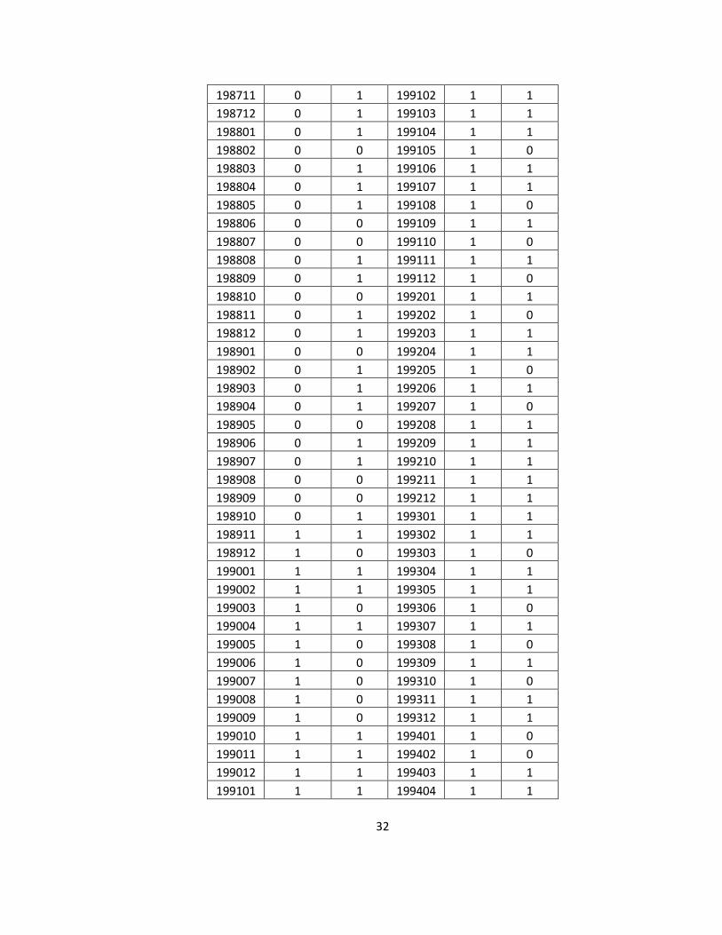
32

198711 0 1 199102 1 1 198712 0 1 199103 1 1 198801 0 1 199104 1 1 198802 0 0 199105 1 0 198803 0 1 199106 1 1 198804 0 1 199107 1 1 198805 0 1 199108 1 0 198806 0 0 199109 1 1 198807 0 0 199110 1 0 198808 0 1 199111 1 1 198809 0 1 199112 1 0 198810 0 0 199201 1 1 198811 0 1 199202 1 0 198812 0 1 199203 1 1 198901 0 0 199204 1 1 198902 0 1 199205 1 0 198903 0 1 199206 1 1 198904 0 1 199207 1 0 198905 0 0 199208 1 1 198906 0 1 199209 1 1 198907 0 1 199210 1 1 198908 0 0 199211 1 1 198909 0 0 199212 1 1 198910 0 1 199301 1 1 198911 1 1 199302 1 1 198912 1 0 199303 1 0 199001 1 1 199304 1 1 199002 1 1 199305 1 1 199003 1 0 199306 1 0 199004 1 1 199307 1 1 199005 1 0 199308 1 0 199006 1 0 199309 1 1 199007 1 0 199310 1 0 199008 1 0 199311 1 1 199009 1 0 199312 1 1 199010 1 1 199401 1 0 199011 1 1 199402 1 0 199012 1 1 199403 1 1 199101 1 1 199404 1 1

33

199405 1 0 199708 1 1 199406 1 1 199709 1 0 199407 1 1 199710 1 1 199408 1 0 199711 1 1 199409 1 1 199712 1 1 199410 1 0 199801 1 1 199411 0 1 199802 1 1 199412 0 1 199803 1 1 199501 0 1 199804 1 0 199502 1 1 199805 1 1 199503 0 1 199806 1 0 199504 1 1 199807 1 0 199505 1 1 199808 1 1 199506 1 1 199809 1 1 199507 1 0 199810 1 1 199508 1 1 199811 1 1 199509 1 0 199812 1 1 199510 1 1 199901 1 0 199511 1 1 199902 1 1 199512 1 1 199903 1 1 199601 1 1 199904 1 0 199602 1 1 199905 1 1 199603 1 1 199906 1 0 199604 1 1 199907 1 0 199605 1 1 199908 1 0 199606 1 0 199909 1 1 199607 1 1 199910 1 1 199608 1 1 199911 1 1 199609 1 1 199912 1 0 199610 1 1 200001 1 0 199611 1 0 200002 1 1 199612 1 1 200003 1 0 199701 1 1 200004 0 0 199702 1 0 200005 0 1 199703 1 1 200006 0 0 199704 1 1 200007 0 1 199705 1 1 200008 0 0 199706 1 1 200009 0 0 199707 1 0 200010 0 0

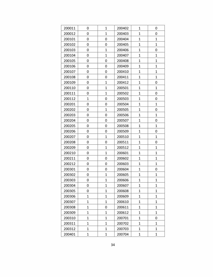
34

200011 0 1 200402 1 0 200012 0 1 200403 1 0 200101 0 0 200404 1 1 200102 0 0 200405 1 1 200103 0 1 200406 1 0 200104 0 1 200407 1 1 200105 0 0 200408 1 1 200106 0 0 200409 1 1 200107 0 0 200410 1 1 200108 0 0 200411 1 1 200109 0 1 200412 1 0 200110 0 1 200501 1 1 200111 0 1 200502 1 0 200112 1 0 200503 1 0 200201 0 0 200504 1 1 200202 0 1 200505 1 0 200203 0 0 200506 1 1 200204 0 0 200507 1 0 200205 0 0 200508 1 1 200206 0 0 200509 1 0 200207 0 1 200510 1 1 200208 0 0 200511 1 0 200209 0 1 200512 1 1 200210 0 1 200601 1 1 200211 0 0 200602 1 1 200212 0 0 200603 1 1 200301 0 0 200604 1 0 200302 0 1 200605 1 1 200303 0 1 200606 1 1 200304 0 1 200607 1 1 200305 0 1 200608 1 1 200306 1 1 200609 1 1 200307 1 1 200610 1 1 200308 1 0 200611 1 1 200309 1 1 200612 1 1 200310 1 1 200701 1 0 200311 1 1 200702 1 1 200312 1 1 200703 1 1 200401 1 1 200704 1 1

35

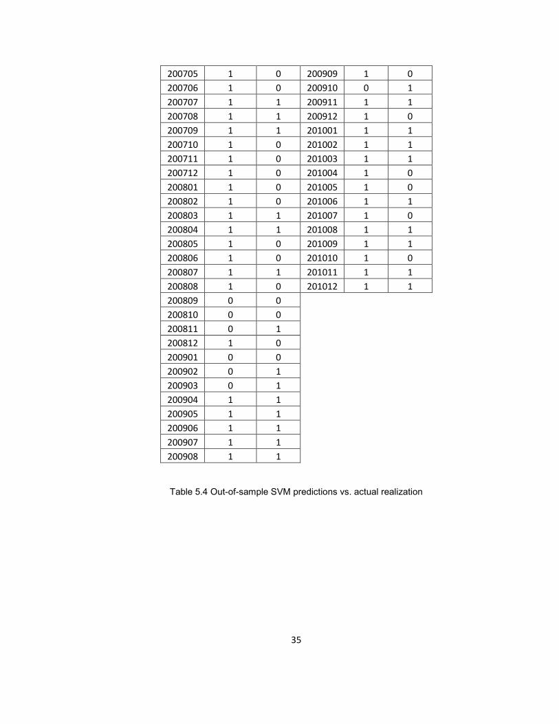
200705 1 0 200909 1 0 200706 1 0 200910 0 1 200707 1 1 200911 1 1 200708 1 1 200912 1 0 200709 1 1 201001 1 1 200710 1 0 201002 1 1 200711 1 0 201003 1 1 200712 1 0 201004 1 0 200801 1 0 201005 1 0 200802 1 0 201006 1 1 200803 1 1 201007 1 0 200804 1 1 201008 1 1 200805 1 0 201009 1 1 200806 1 0 201010 1 0 200807 1 1 201011 1 1 200808 1 0 201012 1 1 200809 0 0 200810 0 0 200811 0 1 200812 1 0 200901 0 0 200902 0 1 200903 0 1 200904 1 1 200905 1 1 200906 1 1 200907 1 1 200908 1 1

Table 5.4 Out-of-sample SVM predictions vs. actual realization

36

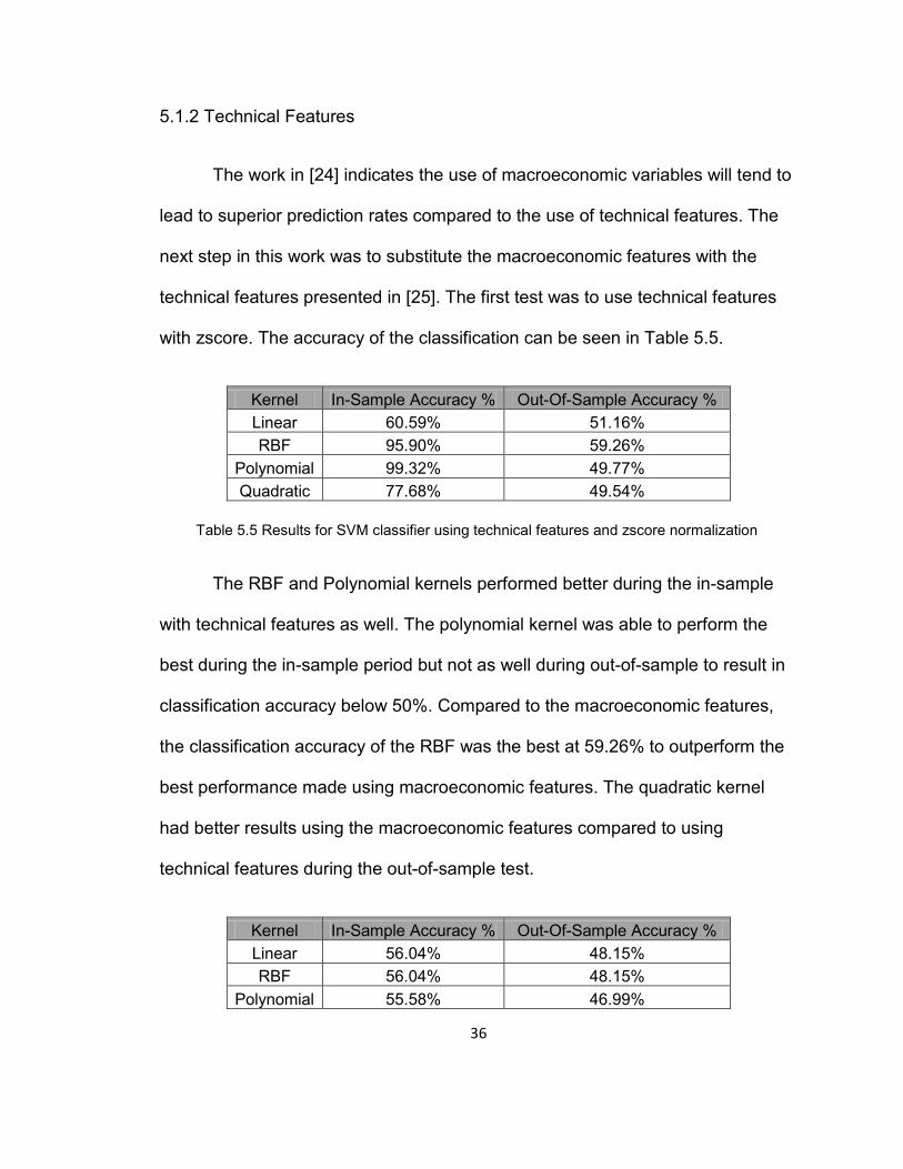
5.1.2 Technical Features

The work in [24] indicates the use of macroeconomic variables will tend to

lead to superior prediction rates compared to the use of technical features. The

next step in this work was to substitute the macroeconomic features with the

technical features presented in [25]. The first test was to use technical features

with zscore. The accuracy of the classification can be seen in Table 5.5.



Table 5.5 Results for SVM classifier using technical features and zscore normalization

The RBF and Polynomial kernels performed better during the in-sample

with technical features as well. The polynomial kernel was able to perform the

best during the in-sample period but not as well during out-of-sample to result in

classification accuracy below 50%. Compared to the macroeconomic features,

the classification accuracy of the RBF was the best at 59.26% to outperform the

best performance made using macroeconomic features. The quadratic kernel

had better results using the macroeconomic features compared to using

technical features during the out-of-sample test.


Polynomial 55.58% 46.99%

37

Quadratic 56.04% 46.99%

Table 5.6 Results for SVM classifier using technical features and normc normalization

Next, the data scaling was tested using normc function and the results

can be seen in Table 5.6. Normc shows very similar performance during the in-

sample and out-of-sample periods. Classification with technical data showed

similar behavior when using the normc to classifying with macroeconomic

features. All kernels had similar results for the in-sample and out-of-sample

The next step was to perform data normalization use the ‘normalize’

function. The polynomial kernel made a noticeable improvement in comparison

with its performance using the normc and zscore functions. It outperformed the

normc function and was able to achieve higher than 50% classification accuracy

during the out-of-sample test period. From Table 5.7, the best performing kernel

was the RBF with 55.56% accuracy during the out-of-sample period.



Table 5.7 Results for SVM classifier using technical features and normalize function

The classification results using zscore are still the best even when using

technical features which are simple to obtain compared to macroeconomic data.

Looking closely at classification results of the best overall performing kernel with

technical features, the RBF with zscore data normalizing, the classifier predicted

38

256 out-of-sample data correctly out of 432. The classifier with technical features

responded well to the short trend oscillation and making classification accuracy

close to 60%. The following table shows detailed results of classification with

technical features and RBF kernel:

yyyymm Prediction Actual 197501 1 1 197707 0 0 197502 1 1 197708 1 0 197503 1 1 197709 0 0 197504 1 1 197710 0 1 197505 1 1 197711 1 1 197506 1 0 197712 1 0 197507 1 0 197801 0 0 197508 1 0 197802 0 1 197509 1 1 197803 1 1 197510 0 1 197804 1 1 197511 0 0 197805 1 0 197512 1 1 197806 0 1 197601 1 0 197807 1 1 197602 1 1 197808 1 0 197603 1 0 197809 1 0 197604 1 0 197810 1 1 197605 1 1 197811 0 1 197606 1 0 197812 1 1 197607 1 0 197901 0 0 197608 1 1 197902 1 1 197609 1 0 197903 0 1 197610 1 0 197904 1 0 197611 1 1 197905 1 1 197612 1 0 197906 1 1 197701 1 0 197907 1 1 197702 0 0 197908 0 1 197703 0 1 197909 1 0 197704 1 0 197910 1 1 197705 1 1 197911 0 1 197706 0 0 197912 0 1

39

198001 1 0 198304 1 0 198002 0 0 198305 0 1 198003 1 1 198306 1 0 198004 1 1 198307 1 1 198005 1 1 198308 1 1 198006 1 1 198309 1 0 198007 1 1 198310 0 1 198008 0 1 198311 1 0 198009 0 1 198312 0 0 198010 1 1 198401 0 0 198011 1 0 198402 1 1 198012 1 0 198403 0 1 198101 1 1 198404 1 0 198102 1 1 198405 1 1 198103 1 0 198406 0 0 198104 0 0 198407 1 1 198105 0 0 198408 1 0 198106 0 0 198409 1 0 198107 0 0 198410 0 0 198108 0 0 198411 1 1 198109 1 1 198412 1 1 198110 1 1 198501 1 1 198111 0 0 198502 1 0 198112 1 0 198503 0 0 198201 0 0 198504 0 1 198202 1 0 198505 1 1 198203 1 1 198506 0 0 198204 1 0 198507 0 0 198205 0 0 198508 1 0 198206 1 0 198509 0 1 198207 0 1 198510 1 1 198208 1 1 198511 1 1 198209 0 1 198512 1 1 198210 1 1 198601 1 1 198211 1 1 198602 1 1 198212 1 1 198603 0 0 198301 1 1 198604 0 1 198302 1 1 198605 0 1 198303 1 1 198606 0 0

40

198607 1 1 198910 1 1 198608 0 0 198911 1 1 198609 1 1 198912 1 0 198610 1 1 199001 1 1 198611 0 0 199002 0 1 198612 0 1 199003 1 0 198701 1 1 199004 0 1 198702 1 1 199005 1 0 198703 1 0 199006 1 0 198704 1 1 199007 0 0 198705 1 1 199008 0 0 198706 0 1 199009 0 0 198707 0 1 199010 1 1 198708 0 0 199011 1 1 198709 1 0 199012 0 1 198710 1 0 199101 1 1 198711 1 1 199102 1 1 198712 1 1 199103 1 1 198801 1 1 199104 1 1 198802 1 0 199105 1 0 198803 1 1 199106 1 1 198804 0 1 199107 1 1 198805 0 1 199108 0 0 198806 1 0 199109 1 1 198807 0 0 199110 0 0 198808 0 1 199111 1 1 198809 1 1 199112 1 0 198810 1 0 199201 0 1 198811 1 1 199202 0 0 198812 0 1 199203 0 1 198901 1 0 199204 1 1 198902 1 1 199205 1 0 198903 0 1 199206 1 1 198904 0 1 199207 0 0 198905 1 0 199208 1 1 198906 0 1 199209 1 1 198907 1 1 199210 1 1 198908 1 0 199211 1 1 198909 0 0 199212 1 1

41

199301 1 1 199604 1 1 199302 1 1 199605 1 1 199303 1 0 199606 1 0 199304 0 1 199607 1 1 199305 1 1 199608 1 1 199306 1 0 199609 0 1 199307 1 1 199610 0 1 199308 0 0 199611 1 0 199309 1 1 199612 1 1 199310 1 0 199701 1 1 199311 1 1 199702 1 0 199312 1 1 199703 1 1 199401 0 0 199704 1 1 199402 1 0 199705 1 1 199403 0 1 199706 1 1 199404 1 1 199707 1 0 199405 1 0 199708 1 1 199406 0 1 199709 0 0 199407 0 1 199710 1 1 199408 1 0 199711 0 1 199409 1 1 199712 0 1 199410 0 0 199801 0 1 199411 0 1 199802 1 1 199412 0 1 199803 1 1 199501 0 1 199804 0 0 199502 1 1 199805 1 1 199503 1 1 199806 0 0 199504 0 1 199807 1 0 199505 0 1 199808 1 1 199506 1 1 199809 1 1 199507 1 0 199810 1 1 199508 0 1 199811 1 1 199509 0 0 199812 1 1 199510 1 1 199901 1 0 199511 0 1 199902 1 1 199512 0 1 199903 1 1 199601 1 1 199904 1 0 199602 1 1 199905 1 1 199603 1 1 199906 1 0

42

199907 0 0 200210 1 1 199908 0 0 200211 1 0 199909 1 1 200212 1 0 199910 1 1 200301 0 0 199911 0 1 200302 0 1 199912 1 0 200303 1 1 200001 1 0 200304 1 1 200002 1 1 200305 1 1 200003 1 0 200306 1 1 200004 0 0 200307 1 1 200005 1 1 200308 1 0 200006 0 0 200309 1 1 200007 1 1 200310 0 1 200008 0 0 200311 1 1 200009 1 0 200312 0 1 200010 0 0 200401 0 1 200011 0 1 200402 0 0 200012 0 1 200403 1 0 200101 1 0 200404 1 1 200102 1 0 200405 1 1 200103 1 1 200406 0 0 200104 1 1 200407 1 1 200105 0 0 200408 1 1 200106 0 0 200409 1 1 200107 0 0 200410 1 1 200108 0 0 200411 0 1 200109 0 1 200412 0 0 200110 0 1 200501 1 1 200111 1 1 200502 0 0 200112 1 0 200503 1 0 200201 0 0 200504 0 1 200202 0 1 200505 1 0 200203 1 0 200506 1 1 200204 0 0 200507 1 0 200205 1 0 200508 1 1 200206 1 0 200509 1 0 200207 1 1 200510 0 1 200208 1 0 200511 1 0 200209 1 1 200512 1 1

43

200601 1 1 200808 1 0 200602 1 1 200809 0 0 200603 1 1 200810 1 0 200604 0 0 200811 1 1 200605 0 1 200812 1 0 200606 0 1 200901 1 0 200607 1 1 200902 1 1 200608 0 1 200903 1 1 200609 1 1 200904 1 1 200610 0 1 200905 1 1 200611 0 1 200906 1 1 200612 0 1 200907 1 1 200701 0 0 200908 1 1 200702 0 1 200909 1 0 200703 1 1 200910 1 1 200704 0 1 200911 0 1 200705 0 0 200912 1 0 200706 0 0 201001 1 1 200707 1 1 201002 1 1 200708 1 1 201003 1 1 200709 1 1 201004 1 0 200710 0 0 201005 1 0 200711 0 0 201006 1 1 200712 0 0 201007 1 0 200801 1 0 201008 1 1 200802 1 0 201009 1 1 200803 1 1 201010 1 0 200804 1 1 201011 1 1 200805 0 0 201012 1 1 200806 1 0 200807 1 1

Table 5.8 Technical Out-of-sample SVM predictions vs. actual realization

44

5.2 SVM RBF Kernel Parameters Selection and Optimization

The next step was to adjust the width of SVM RBF classifier using

parameters C and sigma which will control the margin of classification. One way

to do this is with a grid search method as mentioned in the previous chapters

and papers [27] and [28]. The goal of this search was to find the best pair of

parameters during the in-sample period to maximize the out-of-sample accuracy

as much as possible. The default values for both parameters in Matlab were “1”

for parameters, C and sigma. At the end of our work, the parameter C was not

modified, because once we optimized for the best value of sigma for the RBF

kernel, if we were to modify the parameter C further, it would have resulted in a

softer margin for classification. This will result in slow response of the classifier

(i.e. keeping the classification rate at 1 or 0 for a long period of time).

From Figure 5.1 we notice during optimizing the RBF sigma parameter,

setting the sigma parameter slightly higher than the default, the higher the

accuracy we get. The optimal sigma parameter using macroeconomic features

was 𝑆𝑖𝑔𝑚𝑎 = 0.45 which increased the performance for the out-of-sample

period from 55.79% to 59.25% with zscore data normalizing.

45

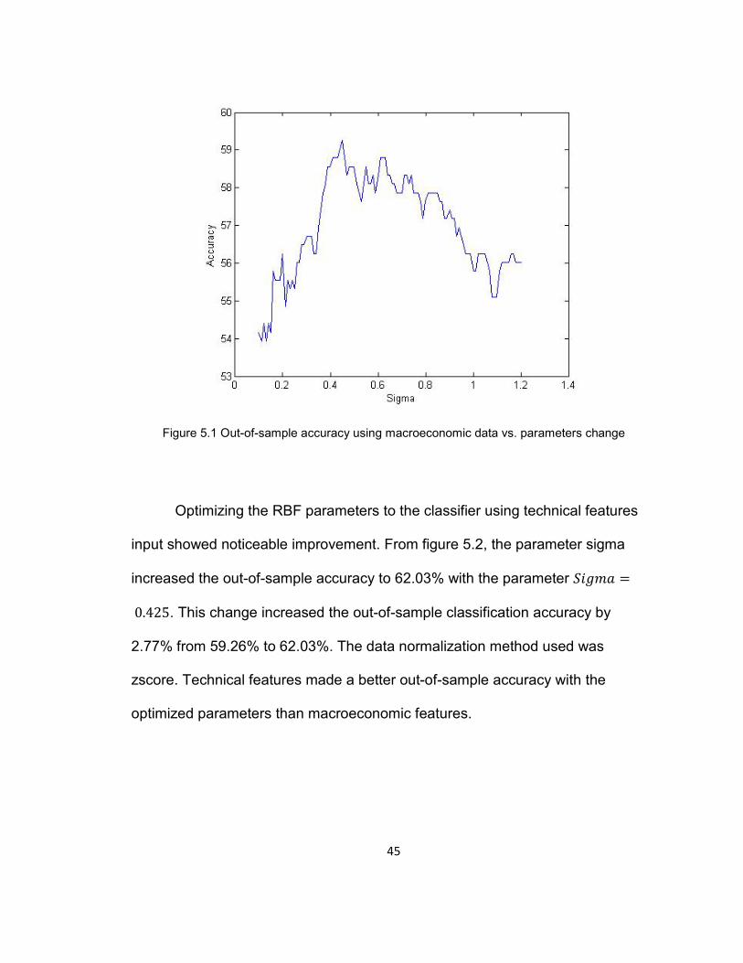
Figure 5.1 Out-of-sample accuracy using macroeconomic data vs. parameters change

Optimizing the RBF parameters to the classifier using technical features

input showed noticeable improvement. From figure 5.2, the parameter sigma

increased the out-of-sample accuracy to 62.03% with the parameter 𝑆𝑖𝑔𝑚𝑎 =

0.425. This change increased the out-of-sample classification accuracy by

2.77% from 59.26% to 62.03%. The data normalization method used was

zscore. Technical features made a better out-of-sample accuracy with the

optimized parameters than macroeconomic features.

46

Figure 5.2 Out-of-sample accuracy using technical data vs. parameters change

5.3 Feature Selection and Dimensionality Reduction

The goal of feature reduction was to reduce the problem dimensionality by

reducing the dataset in order to exclude irrelevant features and at the same time

not have the dataset too small to cause the classifier to be over fit [29].

Sequential Feature Selection and Rankfeatures tests were performed in order to

find the minimum possible features needed. The tests were performed to linear

and RBF kernels since they are used mostly in this kind of work.

47

5.3.1 Sequential Feature Selection

5.3.1.1 Sequential Feature Reduction with Macroeconomic Features

Linear Kernel:

Sequential Feature Selection was performed using the most widely used

two kernels in this sort of application from section 5.1 to both, macroeconomic

and technical features. Table 5.9 shows the features significance using linear

kernel and ‘zscore’ data scaling.

Feature Rank

Feature #

1 14 2 4 3 5 4 7 5 1 6 3 7 15 8 2 9 8

10 10 11 6 12 9 13 13 14 11 15 12

Table 5.9 Macroeconomic Features Significance Ranking using Sequential Feature and linear

kernel

Table 5.10 shows the results of Sequential Feature Selection test using

macroeconomic data, zscore data scaling, and linear kernel.

48

# of Features Out-of-Sample Accuracy 1 60.42% 2 40.50% 3 40.50% 4 40.27% 5 42.13% 6 46.29% 7 45.83% 8 45.83% 9 53.93%

10 53.24% 11 51.15% 12 50.92% 13 50.69% 14 51.38% 15 50.46%

Table 5.10 Sequential Feature Selection for macroeconomic data with Linear Kernel

From the Table 5.10, we notice that only one feature, namely inflation, out

of 15 resulted in the best performance for linear kernel.

RBF Kernel:

Using an RBF kernel gave us different results from the linear kernel.

Using ‘zscore’ when reducing the number of features, we were able to obtain the

best result for macroeconomic with sequential feature reduction where the best

out-of-sample accuracy was 58.33% using 3 features only (TBL, DFR, and DFY)

as seen in Table 5.12. Table 5.11 shows the features significance using RBF

kernel.

49

Feature Rank

Feature #

1 8 2 13 3 12 4 15 5 5 6 10 7 14 8 4 9 7

10 6 11 11 12 3 13 2 14 1 15 9

Table 5.11 Macroeconomic Features Significance Ranking using Sequential Feature and

RBF kernel

# of Features Out-of-Sample Accuracy 1 55.09% 2 55.55% 3 58.33% 4 53.70% 5 54.16% 6 53.93% 7 53.70% 8 53.47% 9 53.70%

10 52.54% 11 52.31% 12 54.39% 13 56.25% 14 55.79% 15 55.79%

50

Table 5.12 Sequential Feature Selection accuracy for macroeconomic data and ‘zscore

normalization and RBF Kernel

5.3.1.2 Sequential Feature Reduction with Technical Features

Linear Kernel:

The significance and ranking of each of the technical features can be

seen in Table 5.13.

Feature Rank

Feature #

1 9 2 15 3 1 4 2 5 3 6 6 7 14 8 10 9 5

10 7 11 4 12 17 13 8 14 16 15 11 16 12 17 13

Table 5.13 Sequential Feature Selection for technical data and linear kernel

Feature reduction with linear kernel and technical features showed an

improvement in the out-of-sample classification that can be seen in Table 5.13.

51

To achieve the best performance for the classifier, less features was given to the

classifier. Using only 2 features (please refer to Table 4.2,) we were able to get

57.87% accuracy. The more features we add, the worse the performance

became.

# of Features Out-of-Sample Accuracy

1 55.78% 2 57.87% 3 56.71% 4 57.17% 5 55.32% 6 54.16% 7 53.70% 8 53.70% 9 54.63%

10 53.24% 11 55.78% 12 53.93% 13 54.63% 14 52.77% 15 52.54% 16 51.62% 17 51.15%

Table 5.14 Sequential Feature Selection for technical data and ‘zscore’ normalization and Linear Kernel

RBF:

Another test of feature reduction was performed to the technical features

but this time using an RBF kernel. Using technical features with RBF kernel, the

more features we added, the better the accuracy we achieved. Classifying using

all features resulted in the best accuracy than classifying with a reduced number

52

of features. The best accuracy achieved was 59.26%. We got the second best

results with only 9 features achieving an accuracy of 58.33%. Table 5.15 shows

the significance features using RBF kernel.

Feature Rank

Feature #

1 1 2 14 3 2 4 8 5 12 6 7 7 3 8 6 9 15

10 17 11 10 12 4 13 9 14 5 15 11 16 16 17 13

Table 5.15 Sequential Feature Selection for technical data and RBF kernel

# of Features Out-of-Sample Accuracy

1 50% 2 50.46% 3 51.85% 4 53.70% 5 54.39% 6 54.16% 7 54.63% 8 58.10% 9 58.33%

53

10 54.63% 11 55.09% 12 54.39% 13 55.55% 14 55.78% 15 57.63% 16 58.33% 17 59.26%

Table 5.16 Sequential Feature Selection for technical data and ‘zscore’ normalization and RBF

Kernel

5.3.2 Rankfeatures

A simpler approach to identify the significant features was to assume all

values are independent and compute a two-way t-test. Computing this test will

return the index with features ranked in order of their effectiveness ranked with

criterion absolute value. This test was used to relate whether the average

difference between two groups was really significant or if it was due instead to

data being random and not associated with each other [30]. We used the Matlab

Rankfeatures function available in the bioinformatics toolbox.

Macroeconomic Features:

Feature Rank

Feature #

1 14 2 11 3 8 4 9 5 10 6 15 7 7

54

8 4 9 2

10 1 11 6 12 13 13 3 14 5 15 12

Table 5.17 Macroeconomic features significance with Rankfeatures

Table 5.17 shows the features significance in order using Rankfeatures.

Feature Rank Out-of-Sample Accuracy 1 60.42% 2 53.24% 3 52.54% 4 52.31% 5 51.85% 6 53.24% 7 53.47% 8 53.24% 9 52.31%

10 53.47% 11 55.78% 12 56.02% 13 56.02% 14 56.02% 15 55.79%

Table 5.18 Rankfeatures Accuracy with macroeconomic features

Table 5.18 shows the accuracy of the classifier with Rankfeatures reducing the

input features with RBF kernel and ‘zscore’ normalizing. Rankfeatures showed

an improvement with the reduced features compared to using all features with

55

macroeconomic by improving the out-of-sample accuracy to 60.42% using the

inflation feature.

Technical Features:

Table 5.19 shows the ranking of features significance for the technical

features.

Ranking Feature 1 3 2 7 3 9 4 16 5 14 6 4 7 5 8 6 9 17

10 2 11 10 12 13 13 1 14 15 15 8 16 12 17 11

Table 5.19 Technical features significance with Rankfeatures

# of Features Out-of-Sample Accuracy 1 50.23% 2 55.79% 3 55.56% 4 56.48% 5 55.56% 6 55.09%

56

7 54.86% 8 56.02% 9 54.86%

10 52.55% 11 54.17% 12 55.79% 13 54.86% 14 56.25% 15 56.48% 16 55.32% 17 59.26%

Table 5.20 Rankfeatures Accuracy with technical features

Table 5.20 shows how technical features did not respond well to

Rankfeatures. Rankfeatures did not identify the significant features in

comparison with Sequential Feature Selection for the technical features. Most of

the out-of-sample accuracies were not close to the best classification result

when including all features. Overall, Rankfeatures worked better with

macroeconomic features compared to technical features.

5.4 Combining Macroeconomic with Technical Features

One of the conclusions in the paper “A Comparison of PNN and SVM for

Stock Market Trend Prediction using Economic and Technical Information,” was

that predicting the market using macroeconomic data was more accurate when

compared to technical indicators [31]. It also contends that the addition of both

macroeconomic and technical features does not improve the classification

accuracy. After running the set of technical features and feature reduction, we

found that the best classification accuracy is achieved when all features are

57

used. Since the more features we add to the RBF classifier, we decided to

expand the initial set of features by combining both the macroeconomic and

technical features. The next step of this work after combining macroeconomic

and technical features was to do a feature reduction to find the best classification

accuracy. When combining all macroeconomic and technical features together,

we were able to obtain 59.72% classification accuracy. This is only marginally

better than using technical features alone.

Procedure Out-of-Sample Accuracy # of Features C Sigma

Combining Macroeconomic with Technical Features 59.72% 32 1 1

Table 5.21 Combination of macroeconomic and technical features

5.5 Summary of Results

Tables 5.22 and 5.23 are a summary of the best performing results and

show a comparison between the experiments using macroeconomic and

technical features alone. Improved accuracies were further obtained optimizing

the SVM RBF parameters. The optimized parameter values are shown in the

tables.

58


All features 56.48% 15 1 1

Sequential Feature Reduction 60.41% 1 1 NA (linear)

Rankfeatures 60.42% 1 1 1 RBF Parameters Optimization 59.25% 15 1 0.45

Table 5.22 Summary of the performance results using macroeconomic features


All features 59.26% 17 1 1 Sequential Feature Reduction 58.33% 9 1 1

Rankfeatures 56.48% 4 1 1 RBF Parameters Optimization 62.04% 17 1 0.425

Table 5.23 Summary of the performance results using technical features

From the above results, we can conclude the overall performance of the

technical features was better than macroeconomic features in contrast to the

result given in [31].

5.6 Comparison between Predictions Based on Basic Assumptions and SVM

The overall trend of the market over the long term is in the up direction.

The next step was to evaluate and compare the classifier prediction

performance during 3 different periods. The first period was the overall out-of-

sample period from January 1975 – December 2010. The two other periods

were when the US economy was hit by financial crisis. The first financial crisis

period considered was from October 2000 – September 2002. This period

represents the period of the bursting of the dot com bubble. The second period

59

was from October 2007 – July 2009, which was during the credit crisis. The

classification was performed using zscore, RBF kernel and technical features.

The first procedure was a comparison of the prediction which assumes a

monthly trend of ‘up’ for all months considered during the out-of-sample period.

Then we did the opposite by comparing the prediction results with down only

during the out-of-sample period. The next procedure was to compare the results

with a naïve prediction where if the previous month was up (or down), then the

next month is predicted to be up (or down). The last procedure was to do the

reverse of the previous procedure where if the previous month was up (or

down), then the next month is predicted to be down (or up).

Procedure Out-Of-Sample Accuracy % Up Only 60.42%

Down Only 39.58% Following Previous Month 52.55%

Opposite of Previous Month 47.22% SVM Prediction 62.04%

Table 5.24 Results for comparing the classification accuracy during the full out-of-sample period

We can see from Table 5.24 that when assuming the index will go up

every month, the overall accuracy was 60.4%. That was true for most of the time

prior to 2000. After that period, the index direction wasn’t going up only but

rather oscillated.

The next step was to compare the results during the first period when the

market crashed. Figure 5.3 shows the index price during the first economic crisis

we were looking at.

60

Figure 5.3 S&P 500 Index price over the first economic crisis (October 2000 – September 2002)

The results of the predictions are provided below:




Table 5.25 Results for comparing the classification accuracy during the first economic

crisis period

From Table 5.25, we can notice if we were to go up only from the

beginning of out-of-sample, a big risk was avoided using SVM for prediction

61

during this economic crisis period if the strategy were to be followed by if the

index price will only go up.

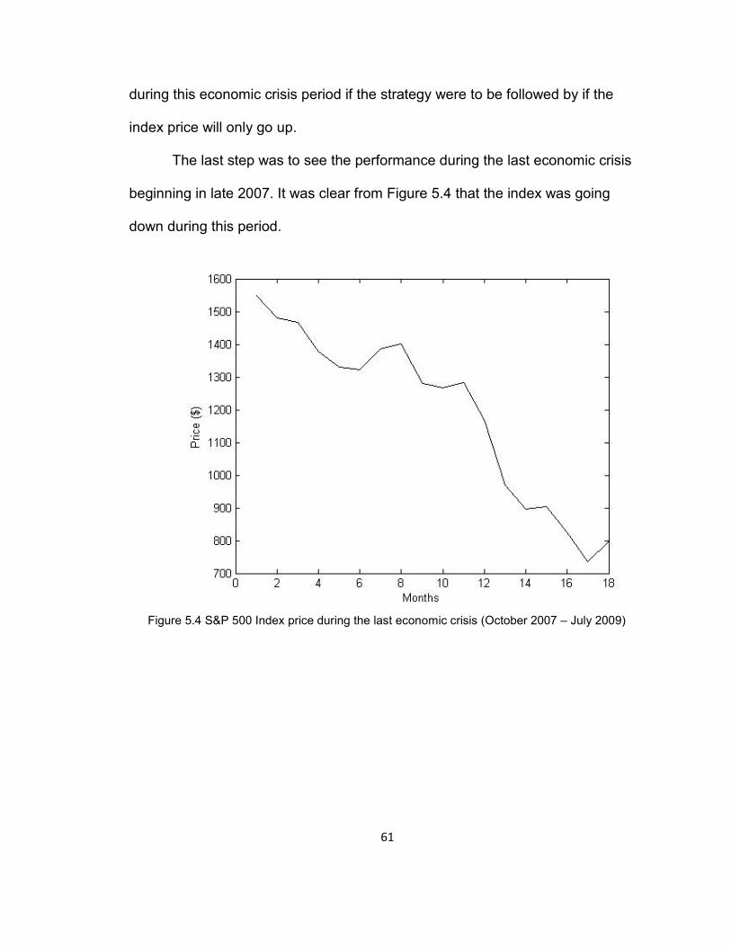
The last step was to see the performance during the last economic crisis

beginning in late 2007. It was clear from Figure 5.4 that the index was going

down during this period.

Figure 5.4 S&P 500 Index price during the last economic crisis (October 2007 – July 2009)

62




Table 5.26 Results for comparing the classification accuracy during the last economic

crisis period

We see from Table 5.26 that if we were to use the up only prediction,

then the accuracy was 33.33%. SVM predicted 61.11% accurately, which as it

happens was the same result when following the direction of previous month.

This was another test to show the advantage of SVM over if we assumed the

market will always go up.

If an investing strategy was implemented during the last two economic

crisis period assuming the market will always go up, it would have encountered

huge losses. The SVM reduced the risk in the first economic crisis to 50%

compared to 58.33% loss when assuming the market will always go up. In the

second economic crisis, SVM gave 61.1% accuracy while an up only strategy

only had 33.33% accuracy.

63

Chapter 6: Conclusion and Future Work

6.1 Conclusion

This worked performed several prediction models using SVM as a

classifying tool in attempt to predict the direction of the market’s trend using S&P

500 into ‘up’ or ‘down’ months. The first model used 15 inputs for

macroeconomic features and 17 for technical features, as inputs to the SVM

classifier. Results showed the best accuracy of 56.48% using all macroeconomic

features with zscore to normalize the data, 51.39% using normc, and 53.94%

using normalize. Classification using technical features showed better results

compared to macroeconomic. We were able to obtain the best classification

accuracy using all technical features with zscore. With normalizing the data

using zscore, we were able to get 59.26% classification accuracy, 49.77% using

normc, and 53.94% using normalize.

Optimizing the RBF’s parameters further and raised the out-of-sample

accuracy from 59.26% to 62.04% using technical features and from 56.48% to

59.25% using macroeconomic features. However, the best result for

macroeconomic data was achieved using only the inflation feature giving

60.42%.

Reducing the dimensionality of the input features using Rankfeatures was

found to be better in terms of choosing the right features needed and the

accuracy to which features to exclude based on the RBF kernel we tested. The

64

response for reducing the features was better for the macroeconomic data. The

linear kernel performs better with fewer features used to classify when using

Sequential Feature Selection. We were able to get 60% accuracy with only one

feature using macroeconomic data.

From this work, we can conclude that classification using technical

features result in better classification accuracy than using macroeconomic

features. This may be fortuitous as obtaining the macroeconomic data is

generally not an easy task. In contrast, technical features can be easily obtained

and since all you need is the index’s price to be able to derive the features used

in this work.

This work was initially motivated by the result presented by Yuan in [24],

where an out-of-sample classification accuracy of 86% was achieved. By the

work done in the thesis we believe this rate of accuracy was achieved

unfortunately by error. Specifically when labeling the correct target, Yuan’s result

is shifted by one month which results in looking into the future. When labeling the

targets in the same way as [24], our classification rate achieved was also 86%

when using technical features and close to 98% with macroeconomic features.

In the future, the parameters of the technical features can be optimized,

perhaps using Genetic Algorithm to find better performing features. Also, SVM

regression can be used to get a sense of what range the index can be expected

to move during prediction period.

65

References

[1] L. Blume and S. Durlauf, The New Palgrave: A Dictionary of Economics,

Second Edition, 2007. New York: Palgrave McMillan.

[2] Kasimati, Evangelia. Macroeconomic and Financial Analysis of Mega-Events.

Thesis. University of Bath, United Kingdom, 2006.

[3] Colby, Robert W. The Encyclopedia Of Technical Market Indicators. 2nd ed.

Toronto: Mc Graw-Hill, 2003.

[4] Sutter, Christian, Zingg, Pascal, and Bertschi, Rolf. Credit Suisse, “Technical

Analysis – Explained.” Accessed August 16, 2013.

[5] Ng, Andrew. Stanford University, “Support Vector Machines.” Accessed

August 2, 2013.

[6] R. Sullivan, A. Timmermann, and H. White. Data-snooping, technical trading

rule performance and the bootstrap. Journal of Finance, 54:1647 – 1691, 1999.

[7] Lento, C., N. Gradojevic, and C. S. Wright. "Investment Information Content

in Bollinger Bands." Applied Financial Economics Letters 3.4 (2007): 263-67.

Print.

[8] Martiny, Karsten. An Investigation of Machine-Learning Approaches for a

Technical Analysis of Financial Markets. Thesis. Technische Universität

Hamburg-Harburg, 2010.

[9] Zhang, Yingjian. Preidiction of Financial Time Serie with Hidden Markov

Models. Thesis. Shandong University, China, 2001.

[10] MQL Community – Technical Analysis, "Momentum." Accessed September

20, 2013. http://ta.mql4.com/indicators/oscillators/momentum

66

[11] OpenCV, "Introduction to Support Vector Machines." Accessed August 10,

2013.

http://docs.opencv.org/doc/tutorials/ml/introduction_to_svm/introduction_to_svm.

html

[12] Bottou, L., and Chih-Jen Lin. National Taiwan University, Department of

Computer Science, “Support Vector Machine Solvers.” (2009).

[13] Weston, J. NEC Labs America, "Support Vector Machine (and Statistical

Learning Theory) Tutorial." Last modified February 26, 2002.

[14] Girma, Henok. Center of Experimental Mechanics. University of Ljubljana.

“A Tutorial on Support Vector Machine.” (2009)

[15] Weisstein, Eric W. "Normalized Vector." From MathWorld--A Wolfram Web

Resource. http://mathworld.wolfram.com/NormalizedVector.html

[16] Bergstra, James, and Bengio, Yoshua (2012). "Random Search for Hyper-

Parameter Optimization". J. Machine Learning Research 13: 281—305.

[17] Chin-Wei Hsu, Chih-Chung Chang and Chih-Jen Lin. A practical guide to

support vector classification. Technical Report, National Taiwan University.

(2010).

[18] Goyal, A., and Welch, I. “A comprehensive look at the empirical

performance of equity premium performance.” Review of Financial Studies 21.

(2008). pp 1455-1508.

[19] TicTacTec, "TA-Lib : Technical Analysis Library." Accessed October 11, 2012. http://www.ta-lib.org/index.html.

[20] Vision, Learning and Robotics, “Feature Normalization for Learning

Classifier.” Accessed September 4, 2013.

http://mathworld.wolfram.com/about/author.html

http://mathworld.wolfram.com/

http://mathworld.wolfram.com/NormalizedVector.html

http://jmlr.csail.mit.edu/papers/volume13/bergstra12a/bergstra12a.pdf

http://jmlr.csail.mit.edu/papers/volume13/bergstra12a/bergstra12a.pdf

http://www.csie.ntu.edu.tw/~cjlin/papers/guide/guide.pdf

http://www.csie.ntu.edu.tw/~cjlin/papers/guide/guide.pdf

http://en.wikipedia.org/wiki/National_Taiwan_University

67

[21] Amibroker, “Walk-forward Testing.” Accessed October 1, 2013.

[22] Fan, J. Fan, Y. and Wu, Y. Princeton University and Harvard University,

“High-Dimensional Classication.” Accessed October 9, 2013.

[23] Scholkopf, B., and Smola, A.J., Learning with Kernels, MIT Press,

Cambridge, MA. 2002.

[24] Yuan, Charles, Washington University in St. Louis, “Predicting S&P 500

Returns Using Support Vector Machines: Theory and Empirics." October 2011.

[25] Teixeira, Lamartine Almeida, and Adriano Lorena Oliveira. "A method for

automatic stock trading combining technical analysis and nearest neighbor

classification." Expert Systems with Application. Vol 37. Oct (2010): 6885-6890.

[26] Vlachos, Andreas. "Active Learning with Support Vector Machines." Thesis.

University of Edinburgh, 2004.

[27] Scikit-learn Developers, "Grid Search: Searching for Estimator Parameters."

http://scikit-learn.org/stable/modules/grid_search.html. Accessed 05 Oct. 2013.

[28] Joachims, Thorsten. Cornell University, “Support Vector and Kernel

Methods.” Accessed September 2, 2013.

3T[29] Hauskrecht, Milos. University of Pittsburgh, “Dimensionality Reduction

Feature Selection.”3T Accessed August 19, 2013.

[30] Weisstein, Eric W. "Paired t-Test." From MathWorld--A Wolfram Web

Resource. Accessed August 11, 2013 http://mathworld.wolfram.com/Pairedt-

Test.html

[31] Lahmiri, Salim. "A Comparison of PNN and SVM for Stock Market Trend

Prediction using Economic and Technical Information." International

Journal of Computer Applications (0975 – 8887). Vol 29, No 3 Sept (2011)

68

[32] Kantavat, P., and Kijsirikul, B., Chulalongkorn University, “Combining

Technical Analysis and Support Vector Machine for Stock Trading.” 2008 IEEE

International Conference on Computational Intelligence for Financial

Engineering.

69

Appendix: Matlab Code

% uses Charles Yuan's macro-economic features clear close all addpath '..\misc' addpath '..\ta-lib-0.0.3_ml2007a-mex_w64' %Prompt User for kernel type prompt = 'Please enter kernel type (linear/rbf/polynomial/quadratic): '; kernel = input(prompt,'s'); % Labels in the Goyal spreadsheet % 1 2 3 4 5 6 7 8 9 10 11 12 13 14 15 16 17 18 % yyyymm Index D12 E12 b/m tbl AAA BAA lty ntis Rfree infl ltr corpr svar csp CRSP_SPvw CRSP_SPvwx % From Yuan paper % 3 4 15 5 10 6 9 13 11 12 % EqPreDir %DP %DY %EP %DE %svar %bm ntis tbl lty ltr TMS %dfy %dfr infl %MA(2,12) %P(t,t-12) A = xlsread('PredictorData2011.xls'); % Amit Goyal's spreadsheet DP = log(A(:,3)) - log(A(:,2)); % 1 DY = [nan;log(A(2:end,3)) - log(A(1:end-1,2))]; % 2 EP = log(A(:,4)) - log(A(:,2)); % 3 DE = log(A(:,3)) - log(A(:,4)); % 4 SVAR = A(:,15); % 5 BM = A(:,5); % 6 NTIS = A(:,10); % 7 TBL = A(:,6); % 8 LTY = A(:,9); % 9 LTR = A(:,13); % 10 TMS = LTY - TBL; % 11 DFY = A(:,8) - A(:,7); % 12 DFR = A(:,14) - LTR; % 13 INFL = A(:,12); % 14 DY12 = [nan(12,1); log(A(13:end,3)) - log(A(1:end-12,2))]; % 15 features=[DP,DY,EP,DE,SVAR,BM,NTIS,TBL,LTY,LTR,TMS,DFY,DFR,INFL,DY12];

70

%features = [EP BM TBL]; % 3, 6, 8 Yuan's best features %%%%%%%%%%%%%%%%%%%%%%%%%%%%%%%%%%%%%%%%%%%%%%%% stk.d = A(:,1); stk.c = A(:,2); CorrectTargets = [stk.c(2:end) >= stk.c(1:end-1); nan]; IS_Start = find(stk.d >= 193806, 1); OOS_Start = find(stk.d >= 197501, 1); OOS_End = find(stk.d >= 201012, 1); IS_Set = features(IS_Start:OOS_Start-1,:); IS_CorrectTargets = CorrectTargets(IS_Start:OOS_Start-1); OOS_Set = features(OOS_Start:OOS_End,:); OOS_CorrectTargets = CorrectTargets(OOS_Start:OOS_End); % In-sample period Normalization Method IS_Set = zscore(IS_Set); % IS_Set = normc(IS_Set); % IS_Set = normalize(IS_Set); svmStruct = svmtrain(IS_Set, IS_CorrectTargets,'autoscale',false,... 'kernel_function',kernel,'method','LS'); YY = svmclassify(svmStruct,IS_Set); errRate = sum(YY ~= IS_CorrectTargets)/length(IS_CorrectTargets); fprintf('inmodel SVM Accuracy: %6.2f %%\n', 100-errRate*100); [r, ~] = size(IS_Set); XX = [IS_Set; OOS_Set]; YY = [IS_CorrectTargets; OOS_CorrectTargets]; for n=1:length(OOS_Set) % choose the desired normalization method XXN = zscore(XX(1:r+n, :)); % XXN = normc(XX(1:r+n, :)); % XXN = normalize(XX(1:r+n, :)); svmStruct = svmtrain(XXN(1:end-1, :), YY(1:r+n-1), ... 'kernel_function',kernel,'autoscale',false,'method','LS'); Results(n, 1) = svmclassify(svmStruct, XXN(end,:)); end

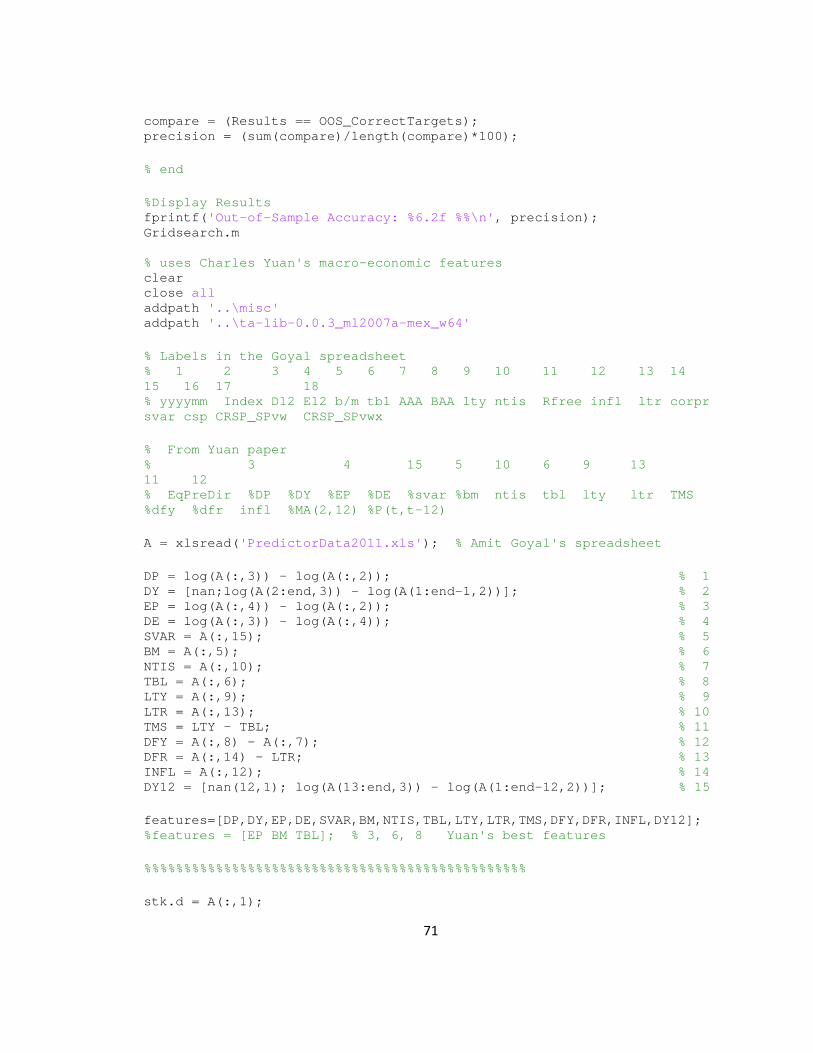
71

compare = (Results == OOS_CorrectTargets); precision = (sum(compare)/length(compare)*100); % end %Display Results fprintf('Out-of-Sample Accuracy: %6.2f %%\n', precision); Gridsearch.m % uses Charles Yuan's macro-economic features clear close all addpath '..\misc' addpath '..\ta-lib-0.0.3_ml2007a-mex_w64' % Labels in the Goyal spreadsheet % 1 2 3 4 5 6 7 8 9 10 11 12 13 14 15 16 17 18 % yyyymm Index D12 E12 b/m tbl AAA BAA lty ntis Rfree infl ltr corpr svar csp CRSP_SPvw CRSP_SPvwx % From Yuan paper % 3 4 15 5 10 6 9 13 11 12 % EqPreDir %DP %DY %EP %DE %svar %bm ntis tbl lty ltr TMS %dfy %dfr infl %MA(2,12) %P(t,t-12) A = xlsread('PredictorData2011.xls'); % Amit Goyal's spreadsheet DP = log(A(:,3)) - log(A(:,2)); % 1 DY = [nan;log(A(2:end,3)) - log(A(1:end-1,2))]; % 2 EP = log(A(:,4)) - log(A(:,2)); % 3 DE = log(A(:,3)) - log(A(:,4)); % 4 SVAR = A(:,15); % 5 BM = A(:,5); % 6 NTIS = A(:,10); % 7 TBL = A(:,6); % 8 LTY = A(:,9); % 9 LTR = A(:,13); % 10 TMS = LTY - TBL; % 11 DFY = A(:,8) - A(:,7); % 12 DFR = A(:,14) - LTR; % 13 INFL = A(:,12); % 14 DY12 = [nan(12,1); log(A(13:end,3)) - log(A(1:end-12,2))]; % 15 features=[DP,DY,EP,DE,SVAR,BM,NTIS,TBL,LTY,LTR,TMS,DFY,DFR,INFL,DY12]; %features = [EP BM TBL]; % 3, 6, 8 Yuan's best features %%%%%%%%%%%%%%%%%%%%%%%%%%%%%%%%%%%%%%%%%%%%%%%% stk.d = A(:,1);

72

stk.c = A(:,2); CorrectTargets = [stk.c(2:end) >= stk.c(1:end-1); nan]; IS_Start = find(stk.d >= 193806, 1); OOS_Start = find(stk.d >= 197501, 1); OOS_End = find(stk.d >= 201012, 1); IS_Set = features(IS_Start:OOS_Start-1,:); IS_CorrectTargets = CorrectTargets(IS_Start:OOS_Start-1); OOS_Set = features(OOS_Start:OOS_End,:); OOS_CorrectTargets = CorrectTargets(OOS_Start:OOS_End); IS_Set = zscore(IS_Set); %%%%%%%%%%%%%%%%%%%%%% X = (0.1:0.01:1.2); Y = (0.1:0.01:1.2); [p,q] = meshgrid(X,Y); pairs = [p(:) q(:)]; tic for j= 1:length(X) j CurrentSigma = X(j) CurrentC = Y(j) svmStruct = svmtrain(IS_Set, IS_CorrectTargets,'autoscale',true,... 'kernel_function','rbf','method','LS','RBF_Sigma',X(j),'boxconstraint',Y(j)); YY = svmclassify(svmStruct,IS_Set); errRate = sum(YY ~= IS_CorrectTargets)/length(IS_CorrectTargets); [r, ~] = size(IS_Set); XX = [IS_Set; OOS_Set]; YY = [IS_CorrectTargets; OOS_CorrectTargets]; for n=1:length(OOS_Set) XXN = zscore(XX(1:r+n, :)); % choose the desired normalization method svmStruct = svmtrain(XXN(1:end-1, :), YY(1:r+n-1), ...

73

'kernel_function','rbf','autoscale',false,'method','LS',... 'RBF_Sigma',X(j),'boxconstraint',Y(j)); Results(n, 1) = svmclassify(svmStruct, XXN(end,:)); end compare = (Results == OOS_CorrectTargets); precision (j) = (sum(compare)/length(compare)*100); CurrentPrecision = precision(end) Pred(j,:) = Results; end toc MaxPrecision = max(precision) % Find the best pair Best = find(precision >= max(precision)); Sigma = X(Best) C = Y(Best) figure(1) % hold on plot(X,precision) ylabel('Accuracy'); % hold off %Display Results fprintf('Out-of-Sample Accuracy: %6.2f %%\n', precision);

74

MacroSequentialFeatureReduction.m % uses Charles Yuan's macro-economic features clear close all addpath '..\misc' addpath '..\ta-lib-0.0.3_ml2007a-mex_w64' %Prompt User for kernel type prompt = 'Please enter kernel type (linear/rbf/polynomial/quadratic): '; kernel = input(prompt,'s'); % Labels in the Goyal spreadsheet % 1 2 3 4 5 6 7 8 9 10 11 12 13 14 15 16 17 18 % yyyymm Index D12 E12 b/m tbl AAA BAA lty ntis Rfree infl ltr corpr svar csp CRSP_SPvw CRSP_SPvwx % From Yuan paper % 3 4 15 5 10 6 9 13 11 12 % EqPreDir %DP %DY %EP %DE %svar %bm ntis tbl lty ltr TMS %dfy %dfr infl %MA(2,12) %P(t,t-12) A = xlsread('PredictorData2011.xls'); % Amit Goyal's spreadsheet DP = log(A(:,3)) - log(A(:,2)); % 1 DY = [nan;log(A(2:end,3)) - log(A(1:end-1,2))]; % 2 EP = log(A(:,4)) - log(A(:,2)); % 3 DE = log(A(:,3)) - log(A(:,4)); % 4 SVAR = A(:,15); % 5 BM = A(:,5); % 6 NTIS = A(:,10); % 7 TBL = A(:,6); % 8 LTY = A(:,9); % 9 LTR = A(:,13); % 10 TMS = LTY - TBL; % 11 DFY = A(:,8) - A(:,7); % 12 DFR = A(:,14) - LTR; % 13 INFL = A(:,12); % 14 DY12 = [nan(12,1); log(A(13:end,3)) - log(A(1:end-12,2))]; % 15 features=[DP,DY,EP,DE,SVAR,BM,NTIS,TBL,LTY,LTR,TMS,DFY,DFR,INFL,DY12];

75

%features = [EP BM TBL]; % 3, 6, 8 Yuan's best features %%%%%%%%%%%%%%%%%%%%%%%%%%%%%%%%%%%%%%%%%%%%%%%% stk.d = A(:,1); stk.c = A(:,2); CorrectTargets = [stk.c(2:end) >= stk.c(1:end-1); nan]; IS_Start = find(stk.d >= 193806, 1); OOS_Start = find(stk.d >= 197501, 1); OOS_End = find(stk.d >= 201012, 1); IS_Set = features(IS_Start:OOS_Start-1,:); IS_CorrectTargets = CorrectTargets(IS_Start:OOS_Start-1); OOS_Set = features(OOS_Start:OOS_End,:); OOS_CorrectTargets = CorrectTargets(OOS_Start:OOS_End); % In-sample period Normalization Method IS_Set = zscore(IS_Set); % IS_Set = normc(IS_Set); % IS_Set = normalize(IS_Set); for k = 1:size(features,2) %%%%%%%%%%%%%%%%%%%%%% % uncomment this section and set NFeatures to limit to top features maxdev = 0.001; opt = statset('display','iter','TolFun',maxdev,'TolTypeFun','abs'); inmodel = sequentialfs(@cfun2,IS_Set,IS_CorrectTargets,... 'cv','none',... 'options',opt,... 'NFeatures', k,... 'direction','forward'); sfsIS_Set = IS_Set(:,inmodel); sfsOOS_Set = OOS_Set(:,inmodel); %%%%%%%%%%%%%%%%%%%%%%%%%%%%%%%%% svmStruct = svmtrain(sfsIS_Set, IS_CorrectTargets,'autoscale',false,... 'kernel_function',kernel,'method','LS'); YY = svmclassify(svmStruct,sfsIS_Set); errRate = sum(YY ~= IS_CorrectTargets)/length(IS_CorrectTargets); [r, ~] = size(sfsIS_Set); XX = [sfsIS_Set; sfsOOS_Set];

76

YY = [IS_CorrectTargets; OOS_CorrectTargets]; for n=1:length(sfsOOS_Set) % choose the desired normalization method XXN = zscore(XX(1:r+n, :)); % XXN = normc(XX(1:r+n, :)); % XXN = normalize(XX(1:r+n, :)); svmStruct = svmtrain(XXN(1:end-1, :), YY(1:r+n-1), ... 'kernel_function',kernel,'autoscale',false,'method','LS'); Results(n, 1) = svmclassify(svmStruct, XXN(end,:)); end compare = (Results == OOS_CorrectTargets); precision(k) = (sum(compare)/length(compare)*100); CurrentPrecision = precision(end) end % # Features and precision [(1:k)' precision']

77

Macrorankfeatures.m % uses Charles Yuan's macro-economic features clear close all addpath '..\misc' addpath '..\ta-lib-0.0.3_ml2007a-mex_w64' %Prompt User for kernel type prompt = 'Please enter kernel type (linear/rbf/polynomial/quadratic): '; kernel = input(prompt,'s'); % Labels in the Goyal spreadsheet % 1 2 3 4 5 6 7 8 9 10 11 12 13 14 15 16 17 18 % yyyymm Index D12 E12 b/m tbl AAA BAA lty ntis Rfree infl ltr corpr svar csp CRSP_SPvw CRSP_SPvwx % From Yuan paper % 3 4 15 5 10 6 9 13 11 12 % EqPreDir %DP %DY %EP %DE %svar %bm ntis tbl lty ltr TMS %dfy %dfr infl %MA(2,12) %P(t,t-12) A = xlsread('PredictorData2011.xls'); % Amit Goyal's spreadsheet DP = log(A(:,3)) - log(A(:,2)); % 1 DY = [nan;log(A(2:end,3)) - log(A(1:end-1,2))]; % 2 EP = log(A(:,4)) - log(A(:,2)); % 3 DE = log(A(:,3)) - log(A(:,4)); % 4 SVAR = A(:,15); % 5 BM = A(:,5); % 6 NTIS = A(:,10); % 7 TBL = A(:,6); % 8 LTY = A(:,9); % 9 LTR = A(:,13); % 10 TMS = LTY - TBL; % 11 DFY = A(:,8) - A(:,7); % 12 DFR = A(:,14) - LTR; % 13 INFL = A(:,12); % 14 DY12 = [nan(12,1); log(A(13:end,3)) - log(A(1:end-12,2))]; % 15 features=[DP,DY,EP,DE,SVAR,BM,NTIS,TBL,LTY,LTR,TMS,DFY,DFR,INFL,DY12]; %features = [EP BM TBL]; % 3, 6, 8 Yuan's best features %%%%%%%%%%%%%%%%%%%%%%%%%%%%%%%%%%%%%%%%%%%%%%%% stk.d = A(:,1); stk.c = A(:,2); CorrectTargets = [stk.c(2:end) >= stk.c(1:end-1); nan];

78

IS_Start = find(stk.d >= 193806, 1); OOS_Start = find(stk.d >= 197501, 1); OOS_End = find(stk.d >= 201012, 1); IS_Set = features(IS_Start:OOS_Start-1,:); IS_CorrectTargets = CorrectTargets(IS_Start:OOS_Start-1); OOS_Set = features(OOS_Start:OOS_End,:); OOS_CorrectTargets = CorrectTargets(OOS_Start:OOS_End); %%%%%%%%%%%%%%%%%%%%%% % uncomment this section and set k to limit to top features for k = 1:size(features,2) [inmodel, Z] = rankfeatures(IS_Set', IS_CorrectTargets, 'NumberOfIndices', k); sfsIS_Set = IS_Set(:,inmodel); sfsOOS_Set = OOS_Set(:,inmodel); %%%%%%%%%%%%%%%%%%%%%%%%%%%%%%%%% % Normalization Method sfsIS_Set = zscore(sfsIS_Set); % sfsIS_Set = normc(sfsIS_Set); % sfsIS_Set = normalize(sfsIS_Set); svmStruct = svmtrain(sfsIS_Set, IS_CorrectTargets,'autoscale',false,... 'kernel_function','rbf','method','LS'); YY = svmclassify(svmStruct,sfsIS_Set); errRate = sum(YY ~= IS_CorrectTargets)/length(IS_CorrectTargets); [r, ~] = size(IS_Set); XX = [sfsIS_Set; sfsOOS_Set]; YY = [IS_CorrectTargets; OOS_CorrectTargets]; for n=1:length(OOS_Set) XXN = zscore(XX(1:r+n, :)); % choose the desired normalization method % XXN = normc(XX(1:r+n, :)); % XXN = normalize(XX(1:r+n, :)); svmStruct = svmtrain(XXN(1:end-1, :), YY(1:r+n-1), ... 'kernel_function','rbf','autoscale',false,'method','LS'); Results(n, 1) = svmclassify(svmStruct, XXN(end,:));

79

end compare = (Results == OOS_CorrectTargets); precision(k) = (sum(compare)/length(compare)*100); CurrentPrecision = precision(end) end % # of features and precision [(1:k)' precision']

80

Technicalfeatures.m % uses technical features clear close all addpath '..\misc' addpath '..\ta-lib-0.0.3_ml2007a-mex_w64' %Prompt User for kernel type prompt = 'Please enter kernel type (linear/rbf/polynomial/quadratic): '; kernel = input(prompt,'s'); A = xlsread('PredictorData2011.xls'); stk.d = A(:,1); stk.c = A(:,2); stk.h = TA_MAX(stk.c,12); stk.l = TA_MIN(stk.c,12); % Calculate Technicals I1 = TA_RSI(stk.c, 14); [bBandsHigh, bBandsMid, bBandsLow] = TA_BBANDS(stk.c,9,2,2); I2 = (stk.c - bBandsHigh)./bBandsHigh; I3 = (stk.c - bBandsLow)./bBandsLow; [stochK, stochD] = TA_STOCHF(stk.h,stk.l,stk.c, 14, 3); I4 = stochK; I5 = stochD; I6 = [nan; diff(stochK)]; I7 = [nan; diff(stochD)]; I8 = [nan; diff(stk.c)./stk.c(1:end-1)]; I9 = (stk.c - stk.l)./(stk.h-stk.l); PMAs = TA_SMA(stk.c,10); PMAl = TA_SMA(stk.c,21); I10 = [nan; diff(PMAs)./PMAs(1:end-1)]; I11 = [nan; diff(PMAl)./PMAl(1:end-1)]; I12 = [nan; (PMAs(2:end)-PMAl(1:end-1))./PMAl(1:end-1)]; I13 = (stk.c - PMAl)./PMAl; I14 = (stk.c - TA_MIN(stk.c,5))./TA_MIN(stk.c,5); I15 = (stk.c - TA_MAX(stk.c,5))./TA_MAX(stk.c,5); MA = (((TA_SMA(A(:,2),2) - TA_SMA(A(:,2),12)) ./ TA_SMA(A(:,2),12))); % 16 MOM = [nan(12,1); (A(13:end,2) - A(1:end-12, 2)) ./ A(1:end-12, 2)]; % 17 features=[I1,I2,I3,I4,I5,I6,I7,I8,I9,I10,I11,I12,I13,I14,I15,MA,MOM]; %%%%%%%%%%%%%%%%%%%%%%%%%%%%%%%%%%%%%%%%%%%%%%%% CorrectTargets = [stk.c(2:end) >= stk.c(1:end-1); nan]; % Choose the testing period

81

IS_Start = find(stk.d >= 193806, 1); OOS_Start = find(stk.d >= 197501, 1); OOS_End = find(stk.d >= 201012, 1); % IS_Start = find(stk.d >= 193806, 1); % OOS_Start = find(stk.d >= 200010, 1); % OOS_End = find(stk.d >= 200209, 1); % IS_Start = find(stk.d >= 193806, 1); % OOS_Start = find(stk.d >= 200710, 1); % OOS_End = find(stk.d >= 200903, 1); IS_Set = features(IS_Start:OOS_Start-1,:); IS_CorrectTargets = CorrectTargets(IS_Start:OOS_Start-1); OOS_Set = features(OOS_Start:OOS_End,:); OOS_CorrectTargets = CorrectTargets(OOS_Start:OOS_End); svmStruct = svmtrain(IS_Set, IS_CorrectTargets,'autoscale',true,... 'kernel_function',kernel,'method','LS'); YY = svmclassify(svmStruct,IS_Set); errRate = sum(YY ~= IS_CorrectTargets)/length(IS_CorrectTargets); [r, ~] = size(IS_Set); XX = [IS_Set; OOS_Set]; YY = [IS_CorrectTargets; OOS_CorrectTargets]; for n=1:length(OOS_Set) % choose the desired normalization method XXN = zscore(XX(1:r+n, :)); % XXN = normc(XX(1:r+n, :)); % XXN = normalize(XX(1:r+n, :)); svmStruct = svmtrain(XXN(1:end-1, :), YY(1:r+n-1), ... 'kernel_function',kernel,'autoscale',false,'method','LS'); Results(n, 1) = svmclassify(svmStruct, XXN(end,:)); end compare = (Results == OOS_CorrectTargets); precision = (sum(compare)/length(compare)*100); conMat = confusionmat(OOS_CorrectTargets,Results); % the confusion matrix %Display Results fprintf('Out-of-Sample Accuracy: %6.2f %%\n', precision);

82

Technical_Gridsearch.m % uses technical features clear close all addpath '..\misc' addpath '..\ta-lib-0.0.3_ml2007a-mex_w64' % %Prompt User for kernel type % prompt = 'Please enter kernel type: '; % kernel = input(prompt,'s'); %Prompt User for Ticker Symbol % prompt = 'Please enter number of features you want to reduce to: '; % no_features = input(prompt); A = xlsread('PredictorData2011.xls'); stk.d = A(:,1); stk.c = A(:,2); stk.h = TA_MAX(stk.c,12); stk.l = TA_MIN(stk.c,12); % Calculate Technicals I1 = TA_RSI(stk.c, 14); [bBandsHigh, bBandsMid, bBandsLow] = TA_BBANDS(stk.c,9,2,2); I2 = (stk.c - bBandsHigh)./bBandsHigh; I3 = (stk.c - bBandsLow)./bBandsLow; [stochK, stochD] = TA_STOCHF(stk.h,stk.l,stk.c, 14, 3); I4 = stochK; I5 = stochD; I6 = [nan; diff(stochK)]; I7 = [nan; diff(stochD)]; I8 = [nan; diff(stk.c)./stk.c(1:end-1)]; I9 = (stk.c - stk.l)./(stk.h-stk.l); PMAs = TA_SMA(stk.c,10); PMAl = TA_SMA(stk.c,21); I10 = [nan; diff(PMAs)./PMAs(1:end-1)]; I11 = [nan; diff(PMAl)./PMAl(1:end-1)]; I12 = [nan; (PMAs(2:end)-PMAl(1:end-1))./PMAl(1:end-1)]; I13 = (stk.c - PMAl)./PMAl; I14 = (stk.c - TA_MIN(stk.c,5))./TA_MIN(stk.c,5); I15 = (stk.c - TA_MAX(stk.c,5))./TA_MAX(stk.c,5); MA = (((TA_SMA(A(:,2),2) - TA_SMA(A(:,2),12)) ./ TA_SMA(A(:,2),12))); % 16 MOM = [nan(12,1); (A(13:end,2) - A(1:end-12, 2)) ./ A(1:end-12, 2)]; % 17 features=[I1,I2,I3,I4,I5,I6,I7,I8,I9,I10,I11,I12,I13,I14,I15,MA,MOM]; %%%%%%%%%%%%%%%%%%%%%%%%%%%%%%%%%%%%%%%%%%%%%%%% stk.d = A(:,1);

83

stk.c = A(:,2); CorrectTargets = [stk.c(2:end) >= stk.c(1:end-1); nan]; IS_Start = find(stk.d >= 193806, 1); OOS_Start = find(stk.d >= 197501, 1); OOS_End = find(stk.d >= 201012, 1); IS_Set = features(IS_Start:OOS_Start-1,:); IS_CorrectTargets = CorrectTargets(IS_Start:OOS_Start-1); OOS_Set = features(OOS_Start:OOS_End,:); OOS_CorrectTargets = CorrectTargets(OOS_Start:OOS_End); %%%%%%%%%%%%%%%%%%%%%% X = (0.1:0.01:1.2); Y = (0.1:0.01:1.2); [p,q] = meshgrid(X,Y); pairs = [p(:) q(:)]; tic for j= 1:length(X) j CurrentSigma = X(j) CurrentC = Y(j) svmStruct = svmtrain(IS_Set, IS_CorrectTargets,'autoscale',true,... 'kernel_function','rbf','method','LS','RBF_Sigma',X(j),'boxconstraint',Y(j)); YY = svmclassify(svmStruct,IS_Set); errRate = sum(YY ~= IS_CorrectTargets)/length(IS_CorrectTargets); [r, ~] = size(IS_Set); XX = [IS_Set; OOS_Set]; YY = [IS_CorrectTargets; OOS_CorrectTargets]; for n=1:length(OOS_Set) XXN = zscore(XX(1:r+n, :)); % choose the desired normalization method svmStruct = svmtrain(XXN(1:end-1, :), YY(1:r+n-1), ... 'kernel_function','rbf','autoscale',false,'method','LS',...

84

'RBF_Sigma',X(j),'boxconstraint',Y(j)); Results(n, 1) = svmclassify(svmStruct, XXN(end,:)); end compare = (Results == OOS_CorrectTargets); precision (j) = (sum(compare)/length(compare)*100); CurrentPrecision = precision(end) Pred(j,:) = Results; end toc MaxPrecision = max(precision) % Find the best pair Best = find(precision >= max(precision)); Sigma = X(Best) C = Y(Best) figure(1) % hold on plot(X,precision) ylabel('Accuracy'); % hold off %Display Results fprintf('Out-of-Sample Accuracy: %6.2f %%\n', precision);

85

TechnicalSequentialFeatureSelection.m % uses technical features clear close all addpath '..\misc' addpath '..\ta-lib-0.0.3_ml2007a-mex_w64' %Prompt User for kernel type prompt = 'Please enter kernel type (linear/rbf/polynomial/quadratic): '; kernel = input(prompt,'s'); A = xlsread('PredictorData2011.xls'); stk.d = A(:,1); stk.c = A(:,2); stk.h = TA_MAX(stk.c,12); stk.l = TA_MIN(stk.c,12); % Calculate Technicals I1 = TA_RSI(stk.c, 14); [bBandsHigh, bBandsMid, bBandsLow] = TA_BBANDS(stk.c,9,2,2); I2 = (stk.c - bBandsHigh)./bBandsHigh; I3 = (stk.c - bBandsLow)./bBandsLow; [stochK, stochD] = TA_STOCHF(stk.h,stk.l,stk.c, 14, 3); I4 = stochK; I5 = stochD; I6 = [nan; diff(stochK)]; I7 = [nan; diff(stochD)]; I8 = [nan; diff(stk.c)./stk.c(1:end-1)]; I9 = (stk.c - stk.l)./(stk.h-stk.l); PMAs = TA_SMA(stk.c,10); PMAl = TA_SMA(stk.c,21); I10 = [nan; diff(PMAs)./PMAs(1:end-1)]; I11 = [nan; diff(PMAl)./PMAl(1:end-1)]; I12 = [nan; (PMAs(2:end)-PMAl(1:end-1))./PMAl(1:end-1)]; I13 = (stk.c - PMAl)./PMAl; I14 = (stk.c - TA_MIN(stk.c,5))./TA_MIN(stk.c,5); I15 = (stk.c - TA_MAX(stk.c,5))./TA_MAX(stk.c,5); MA = (((TA_SMA(A(:,2),2)-TA_SMA(A(:,2),12))./ TA_SMA(A(:,2),12))); % 16 MOM = [nan(12,1);(A(13:end,2) - A(1:end-12, 2))./ A(1:end-12, 2)]; % 17 features=[I1,I2,I3,I4,I5,I6,I7,I8,I9,I10,I11,I12,I13,I14,I15,MA,MOM]; %%%%%%%%%%%%%%%%%%%%%%%%%%%%%%%%%%%%%%%%%%%%%%%% CorrectTargets = [stk.c(2:end) >= stk.c(1:end-1); nan]; IS_Start = find(stk.d >= 193806, 1); OOS_Start = find(stk.d >= 197501, 1); OOS_End = find(stk.d >= 201012, 1);

86

% IS_Start = find(stk.d >= 193806, 1); % OOS_Start = find(stk.d >= 200010, 1); % OOS_End = find(stk.d >= 200209, 1); % IS_Start = find(stk.d >= 193806, 1); % OOS_Start = find(stk.d >= 200710, 1); % OOS_End = find(stk.d >= 200903, 1); IS_Set = features(IS_Start:OOS_Start-1,:); IS_CorrectTargets = CorrectTargets(IS_Start:OOS_Start-1); OOS_Set = features(OOS_Start:OOS_End,:); OOS_CorrectTargets = CorrectTargets(OOS_Start:OOS_End); for k = 1:size(features,2) %%%%%%%%%%%%%%%%%%%%%% % uncomment this section and set NFeatures to limit to top features maxdev = 0.001; opt = statset('display','iter','TolFun',maxdev,'TolTypeFun','abs'); inmodel = sequentialfs(@cfun,IS_Set,IS_CorrectTargets,... 'cv','none',... 'options',opt,... 'NFeatures', k,... 'direction','forward'); sfsIS_Set = IS_Set(:,inmodel); sfsOOS_Set = OOS_Set(:,inmodel); %%%%%%%%%%%%%%%%%%%%%%%%%%%%%%%%% svmStruct = svmtrain(sfsIS_Set, IS_CorrectTargets,'autoscale',false,... 'kernel_function',kernel,'method','LS'); YY = svmclassify(svmStruct,sfsIS_Set); errRate = sum(YY ~= IS_CorrectTargets)/length(IS_CorrectTargets); [r, ~] = size(sfsIS_Set); XX = [sfsIS_Set; sfsOOS_Set]; YY = [IS_CorrectTargets; OOS_CorrectTargets]; for n=1:length(OOS_Set) % choose the desired normalization method XXN = zscore(XX(1:r+n, :)); % XXN = normc(XX(1:r+n, :)); % XXN = normalize(XX(1:r+n, :));

87

% XXN = XX(1:r+n, :); svmStruct = svmtrain(XXN(1:end-1, :), YY(1:r+n-1), ... 'kernel_function',kernel,'autoscale',false,'method','LS'); Results(n, 1) = svmclassify(svmStruct, XXN(end,:)); end compare = (Results == OOS_CorrectTargets); precision(k) = (sum(compare)/length(compare)*100); CurrentPrecision = precision(end) end % # Features and precision [(1:k)' precision']

88

TechnicalRankfeatures.m % uses technical features clear close all addpath '..\misc' addpath '..\ta-lib-0.0.3_ml2007a-mex_w64' % %Prompt User for kernel type % prompt = 'Please enter kernel type: '; % kernel = input(prompt,'s'); %Prompt User for Ticker Symbol % prompt = 'Please enter number of features you want to reduce to: '; % no_features = input(prompt); A = xlsread('PredictorData2011.xls'); stk.d = A(:,1); stk.c = A(:,2); stk.h = TA_MAX(stk.c,12); stk.l = TA_MIN(stk.c,12); % Calculate Technicals I1 = TA_RSI(stk.c, 14); [bBandsHigh, bBandsMid, bBandsLow] = TA_BBANDS(stk.c,9,2,2); I2 = (stk.c - bBandsHigh)./bBandsHigh; I3 = (stk.c - bBandsLow)./bBandsLow; [stochK, stochD] = TA_STOCHF(stk.h,stk.l,stk.c, 14, 3); I4 = stochK; I5 = stochD; I6 = [nan; diff(stochK)]; I7 = [nan; diff(stochD)]; I8 = [nan; diff(stk.c)./stk.c(1:end-1)]; I9 = (stk.c - stk.l)./(stk.h-stk.l); PMAs = TA_SMA(stk.c,10); PMAl = TA_SMA(stk.c,21); I10 = [nan; diff(PMAs)./PMAs(1:end-1)]; I11 = [nan; diff(PMAl)./PMAl(1:end-1)]; I12 = [nan; (PMAs(2:end)-PMAl(1:end-1))./PMAl(1:end-1)]; I13 = (stk.c - PMAl)./PMAl; I14 = (stk.c - TA_MIN(stk.c,5))./TA_MIN(stk.c,5); I15 = (stk.c - TA_MAX(stk.c,5))./TA_MAX(stk.c,5); MA = (((TA_SMA(A(:,2),2)-TA_SMA(A(:,2),12))./TA_SMA(A(:,2),12))); % 16 MOM = [nan(12,1);(A(13:end,2)- A(1:end-12, 2))./ A(1:end-12, 2)]; % 17 features=[I1,I2,I3,I4,I5,I6,I7,I8,I9,I10,I11,I12,I13,I14,I15,MA,MOM]; %%%%%%%%%%%%%%%%%%%%%%%%%%%%%%%%%%%%%%%%%%%%%%%% stk.d = A(:,1); stk.c = A(:,2);

89

CorrectTargets = [stk.c(2:end) >= stk.c(1:end-1); nan]; IS_Start = find(stk.d >= 193806, 1); OOS_Start = find(stk.d >= 197501, 1); OOS_End = find(stk.d >= 201012, 1); IS_Set = features(IS_Start:OOS_Start-1,:); IS_CorrectTargets = CorrectTargets(IS_Start:OOS_Start-1); OOS_Set = features(OOS_Start:OOS_End,:); OOS_CorrectTargets = CorrectTargets(OOS_Start:OOS_End); %%%%%%%%%%%%%%%%%%%%%% % uncomment this section and set k to limit to top features for k = 1:size(features,2) [inmodel, Z] = rankfeatures(IS_Set', IS_CorrectTargets, 'NumberOfIndices', k); sfsIS_Set = IS_Set(:,inmodel); sfsOOS_Set = OOS_Set(:,inmodel); % % feats{inmodel} %%%%%%%%%%%%%%%%%%%%%%%%%%%%%%%%% % Normalization Method % IS_Set = zscore(IS_Set); % IS_Set = normc(IS_Set); % IS_Set = normalize(IS_Set); svmStruct = svmtrain(sfsIS_Set, IS_CorrectTargets,'autoscale',true,... 'kernel_function','rbf','method','LS'); YY = svmclassify(svmStruct,sfsIS_Set); errRate = sum(YY ~= IS_CorrectTargets)/length(IS_CorrectTargets); fprintf('inmodel SVM Accuracy: %6.2f %%\n', 100-errRate*100); [r, ~] = size(IS_Set); XX = [sfsIS_Set; sfsOOS_Set]; YY = [IS_CorrectTargets; OOS_CorrectTargets]; for n=1:length(OOS_Set) XXN = zscore(XX(1:r+n, :)); % choose the desired normalization method % XXN = normc(XX(1:r+n, :)); % XXN = normalize(XX(1:r+n, :));

90

svmStruct = svmtrain(XXN(1:end-1, :), YY(1:r+n-1), ... 'kernel_function','rbf','autoscale',false,'method','LS'); Results(n, 1) = svmclassify(svmStruct, XXN(end,:)); end compare = (Results == OOS_CorrectTargets); precision(k) = (sum(compare)/length(compare)*100); end % # of features and precision [(1:k)' precision']

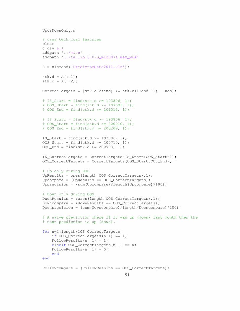
91

UporDownOnly.m % uses technical features clear close all addpath '..\misc' addpath '..\ta-lib-0.0.3_ml2007a-mex_w64' A = xlsread('PredictorData2011.xls'); stk.d = A(:,1); stk.c = A(:,2); CorrectTargets = [stk.c(2:end) >= stk.c(1:end-1); nan]; % IS_Start = find(stk.d >= 193806, 1); % OOS_Start = find(stk.d >= 197501, 1); % OOS_End = find(stk.d >= 201012, 1); % IS_Start = find(stk.d >= 193806, 1); % OOS_Start = find(stk.d >= 200010, 1); % OOS_End = find(stk.d >= 200209, 1); IS_Start = find(stk.d >= 193806, 1); OOS_Start = find(stk.d >= 200710, 1); OOS_End = find(stk.d >= 200903, 1); IS_CorrectTargets = CorrectTargets(IS_Start:OOS_Start-1); OOS_CorrectTargets = CorrectTargets(OOS_Start:OOS_End); % Up only during OOS UpResults = ones(length(OOS_CorrectTargets),1); Upcompare = (UpResults == OOS_CorrectTargets); Upprecision = (sum(Upcompare)/length(Upcompare)*100); % Down only during OOS DownResults = zeros(length(OOS_CorrectTargets),1); Downcompare = (DownResults == OOS_CorrectTargets); Downprecision = (sum(Downcompare)/length(Downcompare)*100); % A naive prediction where if it was up (down) last month then the % next prediction is up (down). for n=2:length(OOS_CorrectTargets) if OOS_CorrectTargets(n-1) == 1; FollowResults(n, 1) = 1; elseif OOS_CorrectTargets(n-1) == 0; FollowResults(n, 1) = 0; end end Followcompare = (FollowResults == OOS_CorrectTargets);

92

Followprecision = (sum(Followcompare)/length(Followcompare)*100); % The reverse of (iii) where if it was up (down) last month then the % next prediction is down (up). for n=2:length(OOS_CorrectTargets) if OOS_CorrectTargets(n-1) == 1; ReverseResults(n, 1) = 0; elseif OOS_CorrectTargets(n-1) == 0; ReverseResults(n, 1) = 1; end end Reversecompare = (ReverseResults == OOS_CorrectTargets); Reverseprecision = (sum(Reversecompare)/length(Reversecompare)*100); %Display Results fprintf('Out-of-Sample Up Only Accuracy: %6.2f %%\n', Upprecision); fprintf('Out-of-Sample Down Only Accuracy: %6.2f %%\n', Downprecision); fprintf('Out-of-Sample Following Accuracy: %6.2f %%\n', Followprecision); fprintf('Out-of-Sample Reverse Accuracy: %6.2f %%\n', Reverseprecision);

93

cfun.m function errRate = cfun(X,Y) % Change to the appropriate kernel svmStruct = svmtrain(X, Y, 'kernel_function', 'linear'); YY = svmclassify(svmStruct,X); errRate = sum(YY ~= Y)/length(Y); % mis-classification rate

94

Normalize.m function data = normalize(d) % the data is normalized so that max is 1, and min is 0 data = (d -repmat(min(d,[],1),size(d,1),1))*spdiags(1./(max(d,[],1)-min(d,[],1))',0,size(d,2),size(d,2));

Documents

Application of Support Vector Machine in Predicting the