Application of surface geophysics to ground water investigations_C_Sismology.pdf

8/12/2019 Application of surface geophysics to ground water investigations_C_Sismology.pdf

http://slidepdf.com/reader/full/application-of-surface-geophysics-to-ground-water-investigationscsismologypdf 1/19

Techniques of Water-Resources Investigations

of the United States Geological Survey

CHAPTER Dl

APPLICATION OF SURFACE GEOPHYSICS

TO GROUND-WATER INVESTIGATIONS

By A. A. R. Zohdy G. P. Eaton

and D. R. Mabey

BOOK 2

COLLECTION OF ENVIRONMENTAL DATA

Click here to return to USGS P

http://localhost/var/www/apps/conversion/tmp/index.html

http://www.usgs.gov/



Seismology

By G. P. Eaton

Applied seismology has, as its basis, thetiming of artificially-generated pulses of

elastic energy propagated through the groundand picked up by electromechanical transducers operating as detectors. These detectors, or geophones as they are m ore commonly called, respond to the motion of theground, and their response, transformed intoelectric signals, is amplified and recorded onmagnetic tape or fi18mon which timing linesare also placed. The geophysicist is inter

ested in two parameters which affect theelapsed time of transmission of this pulse-the propagation velocity (or velocities) andthe geometry of the propagation path. The de-termination of these parameters is a complex task, both in practice and in theory.Energy generated at the meourcetravels inseveral types of waves simultaneously, andeach wave has a different transmission velocity. Furthermore, each of these wavesmay travel to the geophones by more thanone path. For example, the first energy toarrive at a geophone near the source mayarrive via the direct wave ; that is, the energytravels parallel to the surface in the layer in(or on) which the source and receiver arelocated. Another geophone, located fartheraway, may record the arrival of a refractedwave first. When such a wave im’pinges ona sub-horizontal discontinuity where thereis an abrupt change in elastic properties, reflection or refraction of the wave will leadto the generation of additional waves. Thusa compressional wave can give rise to both areflected and refracted compressional wave

and a shear wave. Lastly, energy travellinginto the ground m ay return to the surfacevia reflections or refractions from severaldifferent interfaces of varying depth. Thegeophysicist must be able to recognize amsort out from the complex wave train arriv

ing at the geophones those impulses in whichhe is interested and must translate their1imes of transmission into geological infor-Ination.

Elastic wave energy can be imparted tothe ground in a variety of ways. The mostcommonly used method is that of firing aEharge of explosives with high detonationvelocity in a tamped hole. Such charges maybe fired on the surface or a short distanceabove it. The amoun t of charge used depends on the length of the propagation pathand the attenuation characteristics of theearth material,s along the path. Althoughcrude rules-of-thumb for estimating the explosives requirements for a given shot havebeen formulated, there is enough variationin attenuation characteristics from area toarea that the requirements at a given localeare best determined by trial and error; soalso are the depth-of-shot requirements. Insome areas, and for some kinds of records,the seismologist m ay require a drilled or

augered hole below the water table. In others,he may be satisfied to place the charge in ashallow, hand-dug hole and tamp it with ashovelful of soil. In still others, he may wishto excavate a hole of intermediate depth,say 3-5 m (10-l 5 feet), with a backhoe andthen refill the hole with earth. In general,the deeper the target, the larger the charge,and the larger the charge, the greater depthof implantation. The bulk of the explosiveenergy should be constlmed in producingelastic waves. If much energy is spent in theprocess of venting, the shot probably will

not be efficient and the desired results willnot be obtained. For very shallow work (20

m (65 feet) or less) adequate energy some-

times can be generated by a hamm er blow

on a steel plate. Ana logous sources of energy

67



68 TECHNIQUES OF WATER-RESOURCES INVESTIGATIONS

in larger amounts are produced by weightdropping or by impacting the ground witha plate driven hydraulically.

Elementory Principles

The theory of elasticity on which we baseour understanding of elastic wave propagation treats materials as homogeneous andisotropic. Although naturally occurringrocks, in place, do not fit either specificationvery well in many areas, this theory hasproved to be extremely u’seful in understanding seismic phenomena. Actually, what aresought in seismic prospecting are the verydiscontinuities which make the crust inhomogeneous. These discontinuities, between bodies of unlike elastic properties, are studiedand interpreted in terms of their nature,depth, location, and configuration. In mostearth models they correspond to significantgeological boundaries. In some settings,however, they do not, and this poses an additional problem for the interpreter.

According to the theory of elasticity, ahomogeneous, isotropic, elastic solid cantransmit four kinds of elastic waves. Two ofthese, the compressional (or longitudinal)wave and the shear (or transverse) wave,

are body waves. They are transmittedthrough the interior of the solid. In the pass-age of a compressional wave, particle motion in the medium is parallel to the direction of propagation, like that of a soundwave in air. The particle motion created bya shear wave is perpendicular to the direction of propagation. The other two waves,known as Rayleigh waves and Love waves,are confined to a region near the free surface of the medium; their amplitudes de-crease with depth in the medium. They are

also referred to as surface waves. The particle motion created by these surface waves

is complex ; Love waves, for example, re-quire a surface layer with elastic constantsdifferent from those of the rest of the solid.Very little use has been made of the propagation of shear waves or surface waves in

hydrogeology. However, suggestions havebeen made as to how they might be used toadvantage in ground-water studies (Eatonand Watkins, 1970). Nothing more will besaid of shear or surface waves in the para-graphs that follow-all reference to elastic

wave propagation from this point. on is concerned with compress ional waves. Thesewaves have the highest velocity of the fourtypes discussed and, therefore, the shortesttraveltime for a given propagation path.

Elastic energy moves outward from apoint source in a series of waves with curvedfronts. For illustration, the path which theenergy follows from source to geophone ismost easily defined by a ray, a line drawnnormal, or nearly normal, to the wavefront,depending on whether or not the medium is

isotropic. The ray-paths which seismicenergy follows are constructed by the methodof geometrical optics.

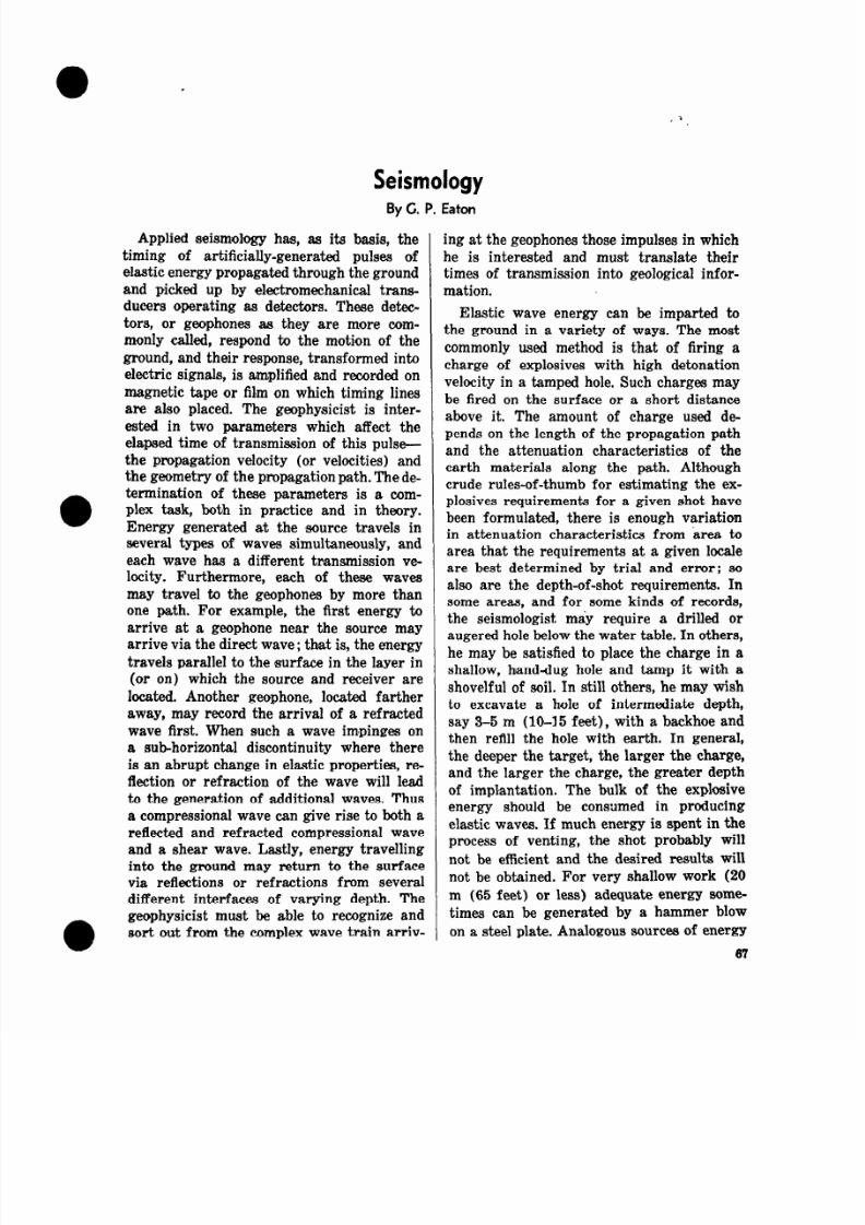
The paths of four rays emanating from apoint source of energy at the ,surface areshown in figure 54. The model is that of ahorizontally layered earth, where the seismicwave velocity, V,, of the upper medium, isless than the velocity of the underlyingmedium, V,. These four rays are:

1. The direct ray, which travels a horizontal path from source to receiver.

2. The totally reflected ray, which is generated when a ray strikes the boundary between the two media at an angleof incidence i, greater than the critical angle i,, and all of thle energy isreflected back toward the surface.

3. A ray striking the boundary at preciselythe critical angle of incide:nce i,, partof the energy being reflected back to-ward the surface and part refracted,the latter travelling parallel to the interface with velocity VI.

4. A ray striking the interface ;at an angleof incidence i’,, less than the criticalangle, part of the energy being reflected upward and part being refractedin the lower medium away from thenormal to the surface, at angle r. Themagnitude of r is a function of the ratio



APPLICATION OF SURFACE GEOPHYSICS 69

t= x------l rWm) GEOPHONE

ENERGY SOURCEG

V, = 3.63 Km/set ’ (3) PATH OF RAY REFRACTED

AlONG VI -V2CONTACT

Figure 54.-Schematic ray-path diagram for seismic energy generated at source S and picked up at geophone G.Traveltimes for the vorious rays are as follows: tl = 0.500 set, tn = 0.630 set, and tr = 0.588 sec.

of the two velocities and the angle ofincidence (see eq. 1). Division of theincident energy between reflected andrefracted waves depends on the angleof incidence and the contrast in velocities and densities of the two media.

As the pulse of energy travelling ray-path3 moves along the interface between thetwo media at velocity V,, it generates a smalldisturbance or pulse in the lowermost part ofthe upper medium. Energy from this disturbance eventually reaches the surface of

the ground where it is picked up by thegeophone.

The angular relationships among the various parts of the ray-paths just described areas follows :

For ray-path 2,i, = iz . (1)

For the reflected branch of ray-path 4,i,’ = iz’, and for the ref,racted #branch

sin i,’ V,- = - (Snell’s Law). (2)Isin r V, .

At the critical angle of incidence, the angleof refraction r is 90” and sin T = 1. Thus,the critical angle can be defined in terms ofthe two velocities as

’ = arcsin V,0( v2 ) *

(3)

These simple equations, .plus that expressing

the relationship between velocity, distance,and time, constitute the basis for the interpretation of seismic data.

As an example, consider the reflected ray-path SR,G. The relationship between the velocity, V,, the length of the propagation path,SR,G, and the transmiss ion time, t is:

vI

= SRs+RaG. (4)

t

Now according to equation 1, i, = iz; thus wecan-rewrite equation 4 as

2 RSsv1=-. (5)

tBecause - -

SR, = v/(X/2) 2 + Z2 ,

then

V 1=

2d(X/2)2+22

t *

Rearranging terms, and solving for 2 :

z = y$ \/V I32 - X ’ . (6)

The distance X in this equation is predetermined by the placement of the geophoneand the transmission time t is read fromthe seismogram. Thus, in equation 6 if thevelocity V,, of the upper medium is knownfrom independent measurement, we can calculate the depth to the interface, 2.




Ref let tion Versus Ref rat tion

.. Shooting

Determination of depth by the meansjust described is referred to as a seismic

reflection measurement. The reflection method is one of two general types of seismicmeasurements in mmmon use, the other being the refraction method.

The refraction method is illustrated schematically by ray-path 3 in figure 54. Thepropagation path of ray 3 consists of three

branches, %,, R,R,, and R,G, but we havenot yet indicated why there should be a

branch like R,G. It was mentioned earlierthat energy from the disturbance travelling

along path R,R, eventually reaches the sur

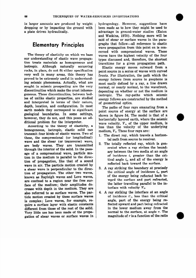
face. The head wave, which is the name givento the wave carrying energy upward fromthe disturbance at the interface, is a physical representation of Huygens’ principle,which states that each point on an advancing wave front in an ideal elastic body is asource of second,ary spherical waves. Thewave front of thee new waves at a laterinstant of time is defined by a surface tan-gent to the newly-generated spherical waves.This is illustrated in figure 55 , where a, b,and c represent successive crests of a disturbance moving parallel to the interfacewith velocity V,. They are, according toHuygens’ pri&ple, sources of secondarywaves which will move upward in the disturbed utiper medium with velocity V,. The

arc3 in figure 55 represent a succession ofspherical waves emanatiag from each of thesepoints and the thin lines tangent to them arethe wave fronts normal to which the raystravel. As a disturbance with velocity V,travels parallel to the interface from a to c,energy radiating upward from it travelsfrom a to d at velocity V,. These two paths,

E and ad, define the angle W.Thus,

ii-3 v,t VI&lo = ---=-. (7)

ac v*t v,

TeNGENT TO SPHERICAL WAVE FRONTS

“I

SPHERICAL WAVE FRON@R’y PArH OF nEAD WAVE

a c

“2

Figure 55 .-Huygens’ construction for a head wave

generoted at the VI-V2 inte rface.

as the critical angle i,. The significance ofthis in figure 54 is that the right hand

branch of ray-path 3 or R,G i,s a mirror

image of the left-hand or incident branchSR,. It follows tha t the relationship betweenthe velocities V, and V, ,the length of the

propagation path SR,R,G, and the transmission time t can be written

- -2SRz RzR,

t= -+-.VI VR

The geometry of figure 54 allowsthe following substitutions :

SRz = Z/ cos i,and

R,R,=X-222tani,.

us to make

(9)

(10)

Suhetituting these expressions ,and that ofequation 3 in equation 8 leads to

22 cos i,t= (11)

v, -

After rearrang ing terms, and sutitutingan expression containing V, and V, forcos i, :

2= 2g*2

vivz- v,*

(t-x/%). (12)

As before, the distance X is predeterminedby the pl,acement of the geophone and the

transmission time t is read from the seismogram. Substitutions of these values, plusthose for V, and Vz, in equation :L2 leads toa value for ,the depth 2 to the interface.

A comparison of equation ‘7 with equation In making calculations of deptlh from re

3 indicates that the the angle o is the same flection measurements, the velocity values



0 APPLICATION OF SURFACE GEOPHYSICS 71

used must be determined by independen tmeans. In contrast, refraction measurementsyield values for the velocities of <the formations directly, provided certain conditionsare realized. Although a discussion of theseconditions is beyond the scope of the manual,

it may be instructive to show how the valuesfor velocities V, and V, are a product of therefraction measurement itself.

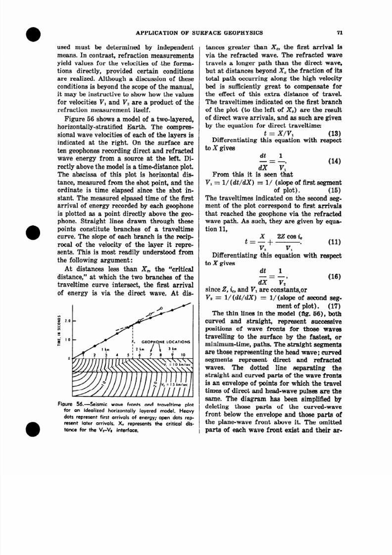
Figure 56 shows a model of a two-layered,horizontally-stratified Earth. The compressional wave velocities of each of the layers isindicated at the right. On the surface a reten geophones recording direct and refractedwave energy from a source at the left. Directly #abovehe ‘model is a time-distance plot.The abscissa of this plot is horizontal distance, measured f,rom the shot point, and the

ordinate is time elapsed since the shot instant. The measured elpased time of the firstarrival of energy recorded ‘by each geophoneis plotted as a point directly above the geophone. Straight dines drawn through thesepoints constitute #branches of a traveltimecurve. The slope of each branch is the reciprocal of the velocity of the ,layer it rep resents. This is most readily understood fromthe following argument :

At distances less than XC, the “criticaldistance,” at which the two branches of thetravel(time curve intersect, the first arrival

of energy is via the direct wave. At dis

;;’ IOGEOPHONE LOCATIONS

F

S

Figure 56.~Seismic wave fronts and traveltime plot

for an idealized horizontally layered model. Heavy

dots represent first arrivals of energy; open dots rep

resent later arrivals. X0 represents the critical dis

tance for the K-V, interface.

tances greate r than XC, the first arrival isvia the refracted wave. The refracted wavetr,avels a longer path than the direct wave,but at distances beyond X, the fraction of itstotal path occurring along the high velocitybed is sufficiently great to compensate for

the effect of thi,s extra distance of travel.The traveltimles indicated on the first branchof the plot (to the left of XC) are the resultof direct wave arrivals, and as such are givenby the equation for direct traveltime:

t = x/v, (13)Differentiating this equation with respec t

to X givesdt 1- = -. (14)dX V,

From this it is seen thatV, = l/ (dt/dX) = l/ (slope of first segment

of plot).(15)The tr,aveltimes indicated on the second seg

ment of the plot correspond to first arrivalsthat reached the geophone via the refractedwave ,path. As such, they are given by equa.tion 11,

22 cos i,t= ;+ v * (11)

Differentiating It&s equahon with respectto X gives

dt 1-=-) (16)dX V,

since 2, iC,and V, are com&ants,orVz = l/(dt/dX) = l/(slope of second seg

ment of plot). (17)The thin lines in the model (fig. 56), both

curved and straight, represent successivepositions of wave fronts for those wavestraveHing ato the surface by the fastest, orminimum-time, paths. Tlhe straight segmentsare those representing the head wave; curvedsegments represent direct ,and refractedwaves. The dotted line separating thestraight and curved pa rts of the wave frontsis an envelope of points for which the traveltimes of direct and head-wave pulses are thesame. The diagram has been simplified bydeleting those parts of the curved-wavefront ,below the envelope and those parts ofthe plane-wave front above it. The omittedparts of each wave front exist and their ar-




rival at the geophones constitutes a laterarrival of real energy. Thus one may see onthe seismogram at geophones 6, 7,and 8, aninstant after the head-wave arrival, pulsesthat represent the arrival of a direct wavetravelling w&h velocity V,. These are shown

in figure 56 as open circles falling on a prolongation of the V, traveltime branch. Suchpulses are known as secondarrivals. Becausethe amplitude of a head wave usually is muchsmaller than that of ,a di,rect wave, it veryrarely is observed on the seismograms at distances less than the critical distance.

Comparison of the

Reflection and Refraction

Seismic Methods in Practice

In the preceding paragraphs, simple techniques of depth measurement by both thereflection and refraction methods have beendescribed. Hbw does one go about decidingwhich method to use in a given situation?The differences between reflection and re-fraction methods go far beyond the differencesin ray-path geometry. These differencesinclude geophone array (the refractionmethod uses much longer spreads), accuracy, resolution, depth, size and shape of the

target, number of discontinuities to bemapped, vertical succession of velocity varues, and cost. The great bulk of all appliedseismic work done today is done by the reflection method. It offers higher accuracy andresolution, allows the mapping of a largernumber of horizons, requires smaller amountiof energy, uses shorter geophone spreads(simplifying their layout and minimizingproblems msociated with the communicationof the shot instant), and is more amenableto routine field operation. In addiltion it doesnot require, as does the refraction method,

that each succeeding layer have a velocityhigher than that of the layer above it. Inlight of all these advantages, it is reasonableto inquire why the refraction method is usedat all. This is an especially relevant questionhere, because most seismic measurements

made in ,hydrogeology are refraction measurements. It is in petroleum exploration thatthe reflection method is so extensively used.

The reasons for use of the refraotionmethod are several. In some areas it is almost impossible to obtain good reflection rec

ords. A typ ical example is an area of thickalluvial or glacial fill. In this settin,g optimumreflection prospecting would require thedrilling of deep shot holes. Such an area lendsitself admirably to the refraction methodand is precisely the kind of settin:g in whichthe hydrogeologist might be interested. Adownward increase in velocity can be reacsonably expected in such an area and abruptincreases in velocity might be encounteredboth at the water table and at the base ofthe sediments, if they overlie consolidatedbedrock. No prior knowledge of velocity is

required in reconnaissance refraction measurements and the velocity information obtained in the course of the work may helpin identifying the rock types involved. Inreflection shooting special measurements ofvelocity to be made, either by greatly expanding an occasional geophone spread or byshooting at a well into which a geophone hasbeen lowered. In the exploration of a largealluvial basin such wells may not be availableto the seismologist. The reflection methodworks best when continuous line coverage i,s

possible and when the line or lines can betied to,a few points of velocity control. A single reflection profile, or a series of them individually isolated and spread over manysquare kilometers of an alluvial basin, arenot as useful as a series of isolated refraction profilee.

In areas where steeply dipping boundariesare encountered, the refraction .method isbettek suited for exploration than the reflection method. Typical examples include afault-bounded valley or a buried valley withsteeply sloping sides.

The sophisticated equipment u 3ed in reflection work today, the relatively large sizeof the crews required, and the benefit,s de-rived from continuous coverage, a.re all difficult to justify in relation to the objectiveaand budget of a typical ground-waker study.




The geometric subtlety of the target andthe ultimate economic returns from successful explora tion for petroleum do justify itsuse in the oil industry.

Seismic RefractionMeasurements in

H yd rog eology

Effect of Departures From the

Simple Stratified Model

The models shown in figures 54 and 56 arehighly simplified. The ground surface is perfectly plane and horizontal, the surface ofthe refractor with velocity V, is also plane,and the two surfaces are parallel. In addition, there is but one velocity discontinu ityto map and there are no lateral or verticalmriations of velocity within either layer.The ray-path geometry and the equationsfor calculating depths to the lower refractorare therefore equally simple. Such simplicityis seldom encountered in nature. The complications of real systems can be illustratedby some hypothetical models and time-distance plots.

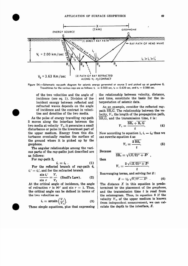
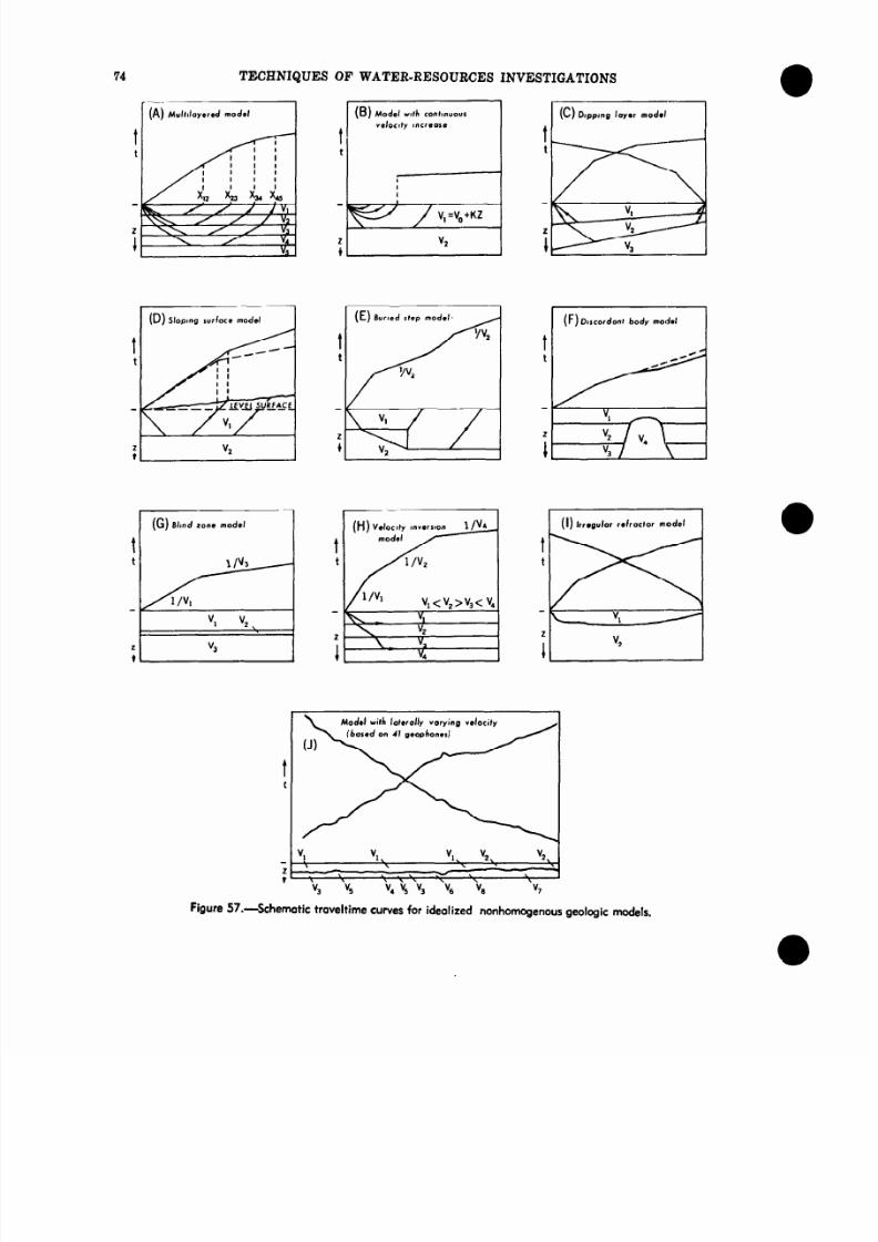
Figure 57 shows 10 models which departin significant ways from the simple models

of figures 54 and 56. Immediately above eachmodel is a schematic time-di’stance plot typical of the type that the model would generate. Bay paths are shown for models Athrough E, and also for model H.

The Multilayered Model

Figure 57A

Although this mode l is a simple extensionof the horizontal two-layer model, its interpretation ie f,raught with practical difficulty.The thickness of each succeeding layer mustbe calculated individually ‘employing a seriesof formulas into which one substitutes valuesderived for the layer immediately above it.Small errors in each step of the analysishave a multiplier effect which carries ove r tothe calculations on each succeeding layer.

This model also requires that each layer havea velocity higher than the one above it (seefig. 57H) and that each be thick enough toproduce a separate branch of the traveltimecurve (see fig. 67G).

Effect of a Regular Increase of VelocityWith Depth

Figure 57B

If the layers in A become vanishinglythin, they would approximate, as a group,a continuous velocity increase with depth.The result is the generation of a curved raypath in the upper medium. Such a situationis realized in thick sections of young, semi-consolidated sedimentary rocks which display increasing compaction and lithificationwith depth. Several velocitydepth functionshave been proposed by investigators for different areas (Dobrin, 1960, p. 77 ; Kaufmann,1953, table 1). The mathematics required forthe calculation of depth to a lower bedrockrefractor using these equations are simpleenough for analytical treatment in some situations.

Effect of Dipping Layers

Figure 57C

This model illustrates the effect of a re

fractor that is not parallel to the surface ofthe ground. Geologically, this model corresponds to a series of dipping beds or to asloping bedrock surface. In this situation theslopes of the separate branches of the travel-time curves give reciprocal values of velocityfor the uppermost ,layer (V,) only. In figure57C, the slopes of the second and thirdbranches of the traveltime curves are notreciprocals of velocities Vz and V,. Theseslopes also are not the same for the two directions of shooting (left to right, or updip,and right to left, o r downdip). If a seismicprofile in a geologic setting like this one werenot reve rsed ; that is, if it were not shot firstfrom one end of the geophone spread andthen from the other, there would be no wayof recognizing the dip nor the erroneousvalues for V, and Vs. By reve rsing the pro-



TECHNIQUES OF WATER-RESOURCES INVESTIGATIONS

0) Slopmg surface model Burled step model. 1(F)orcordont body model1t

t

(G) Blond zone model /HI Valoc,ty I”“=‘-‘“” 1 I” (I) ~rr.gdor refractor modal

Model with loterolly varying velocity

(bared on II geophonesl

tt

Figure 57.-Schematic traveltime cu rves for idealized nonhomogenous geo logic models.




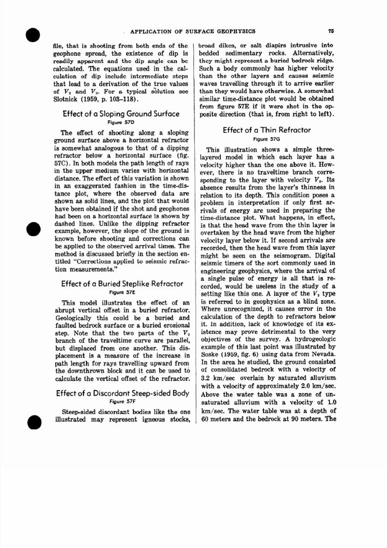
file, that is shooting from both ends of thegeophone spread, the existence of dip isreadily ‘apparent and the dip angle can becalculated. The equations used in the calculation of dip include intermediate stepsthat lead to a derivation of the true va luesof V, and V,. For a typical &lution seeSlotnick (1959, p. 103-118).

Effect of a Sloping Ground SurfaceFigure 57D

The effect of shooting along a slopingground surface above a horizontal refractoris somewhat analogous to that of a dippingrefractor below a horizontal surface (fig.5%). In both models the path length of raysin the upper medium varies with horizontaldistance. The effect of this varia tion is shownin an exaggerated fashion in the time-dis

tance plot, where the observed data areshown as solid lines, and the plot that wouldhave been obtained if the shot and geophonhad been on a horizontal surface is shown bydashed lines. Unlike the dipping refractorexample, however, the slope of the ground isknown before shooting and corrections canbe applied to the observed arrival times. Themethod is discussed briefly in the section en-titled “Corrections applied to seismic refraction measurements.”

Effect of a Buried Stepli ke RefractorFigure 57E

This model illustrates the effect of anabrupt vertical offset in a buried refractor.Geologically this could be a buried andfaulted bedrock surface or a buried erosionalstep. Note that the two parts of the V,branch of the traveltime curve are parallel,but displaced from one another. This displacement is a measure of the increase inpath length for rays travelling upward fromthe downthrown block and it can be used tocalculate the vertical offset of the refractor.

Effect of a Discordant Steep-sided BodyFigure 57F

Steep-sided discordant bodies like the oneillustrated may represent igneous stocks,

broad dikes, or salt diapirs intrus ive intobedded sedimentary rocks. Alternatively,they might represent a buried bedrock ridge.Such a body commonly has higher velocitythan the other layers and causes seismicwaves travelling through it to arrive earlierthan they would have otherwise. A somewhatsimilar time-distance plot would be obtainedfrom figure 57E if it were shot in the opposite direction (that is, from right to left).

Effect of a Thin Refractor

Figure 57G

This illustration shows a simple three-layered model in which each layer has avelocity higher than the one above it. How-ever, there is no traveltime branch corresponding to the layer with velocity V,. Itsabsence results from the layer’s thinness inrelation to its depth. This cond ition poses aproblem in interpretation if only first arrivals of energy are used in preparing thetime-distance plot. What happens, in effect,is that the head wave from the thin layer i,sovertaken by the head wave from the highervelocity layer below it, If second arrivals arerecorded, then the head wave from this layermight be seen on the seismogram. Digitalseismic timers of the sort commonly used inengineering geophysics, where the arrival ofa single pulse of energy is all that is re-

corded, would be useless in the study of asetting like this one. A layer of the Vz typeis referred to in geophysics as a blind zone.Where unrecognized, it causes error in thecalculation of the depth to refractors belowit. In addition, lack of knowledge of its existence may prove detrimental to the veryobjectives of the survey. A hydrogeologicexamp le of this last point was illustrated bySoske (1959, fig. 6) using data from Nevada.In the area he studied, the ground consistedof conso lidated bedrock with a velocity of

3.2 km/set overlain by saturated alluvium.

with a velocity of approx imately 2.0 km/set.

Above the water table was a zone of unsaturated alluvium with a velocity of 1.0

km/set. The water table was at a depth of

60 meters and the bedrock at 90 meters. The




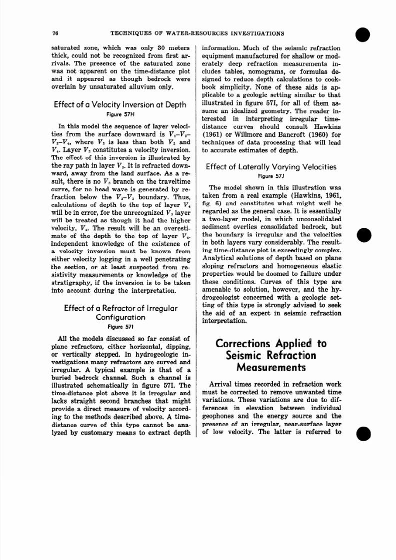
saturated zone, which was only 30 metersthick, could not be recognized from first arrivals. The presence of the saturated zonewas not-apparent on the time-distance plotand it appeared as though bedrock wereoverlain by unsaturated alluvium only.

Effect of a Velocity inversion at Depth

Figure 57H

In this model the sequence of layer velocities from the surface downward is VI-V,-V,-V,, where V, is less than both V, andV,. Laye r V , constitutes a velocity inversion.The effect of this invers ion is illustrated bythe ray path in layer V,. It is refracted down-ward, away from the land surface. As a result, there is no V, branch on the traveltimecurve, for no head wave is generated by re-

fraction below the V,-V, boundary. Thus,calculations of depth to the top of layer V,will be in error, for the unrecognized V, layerwill be treated as though it had the highervelocity, V,. The result will be an overestimate of the depth to the top of layer V4.Independent knowledge of the existence ofa velocity inversion must be known fromeither velocity logging in a well penetratingthe section, or at least suspected from resistivity measurements or knowledge of thestratigraphy, if the inversion is to be taken

into account during the interpretation.

Effect of a Refractor of Irregular

Configuration

Figure 571

All the models discussed so far consist ofplane refractors, either horizontal, dipping,or vertically stepped. In hydrogeologic investigations many refractors are curved andirregular. A typical example is that of aburied bedrock channel. Such a channel isillustrated schematically in figure 571. The

timedistance plot above it is irregular andlacks straight second branches that mightprovide a direct measure of velocity according to the methods described above. A time-distance curve of this type cannot be analyzed by customary means to extract depth

information. Much of the seismic refractionequipment manufactured for shallow or modera,tely deep refraction measurements includes tables, nomograms, or formulas designed to reduce depth calculations to cook-book simplicity. None of these aids is ap

plicable to a geologic setting similar to thatillustrated in figure 571, for all of them assume an idealized geometry. The reader interested in interpreting irregular time-distance curves should consult Haw-kins(1961) or Willmore and Bancroft (1960) fortechniques of data processing that will leadto accurate estimates of depth.

Effect of Latera lly Varying Velocities

Figure 57J

The model shown in this illustration was

taken from a real example (Haywkins, 1961,fig. 6) and constitutes what might well beregarded as the general case. It is essentiallya tw.o-layer model, in which unconsolidatedsediment overlies consolidated bedrock, butthe boundary is irregular and the velocitiesin both layers vary considerably. The resulting time-distance plot is exceedingly complex.Analytical solutions of depth based on planesloping refractors and homogeneous elasticproperties would be doom8edto failure underthese conditions. Curves of this type areamenable to solution, however, and the hydrogeologist concerned with a geologic setting of this type is strongly advised to seekthe aid of an expert in seismic refractioninterpretation.

Corrections Applied toSeismic Ref ractiion

Measuflements

Arrival times recorded in refraction work

must be corrected to remove unwanted timevariations. These variations are due to differences in elevation between individualgeophones and the energy soulrce and thepresence of an irregular, near-surface layerof low velocity. The latter is referred to




a

commonly as the weathered layer, althoughthis name may or may not be strictly COKrect geologically.

Elevation Correction

The simplest means of correcting for d ifferences in elevation between the geophonesand the shot is to convert them all to a common elevation datum by subtracting or adding the times that elastic waves would taketo travel from the datum to the actualgeophone or shot locations. A schem*atic ex-ample is shown in figure 57D. This requiresknowledge of the elevation of shot and geophones and of the velocity of the mediumbetween them and the datum. The velocityis readily obtained from refraction shooting.

Weathered-layer Correction

If an irregu lar l,ow-velocity layer existsimmediately beneath the surface, but is nottaken into account in correcting the travel-time data, the effect will be to produce artifical variations in depth to a mapped refractor such as the buried bedrock surface. Thesimplest means for making this correction isto shoot it with short geophone spreads and

calculate its thickness and velocity by conventional methods. This information then canbe used to calculate the time delays whichthe weathered layer causes along those partsof the ray path near the surface, both at theshot point and at the geophones.

Errors in Seismic Refraction

Measurements

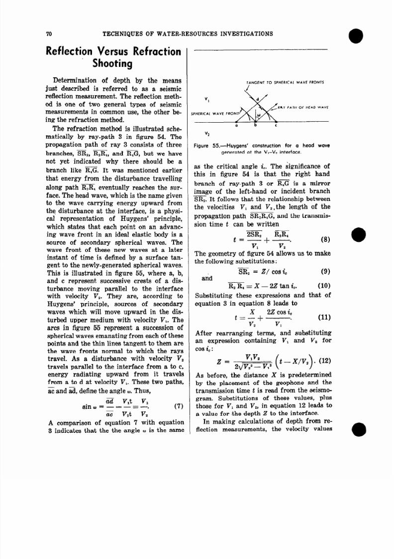
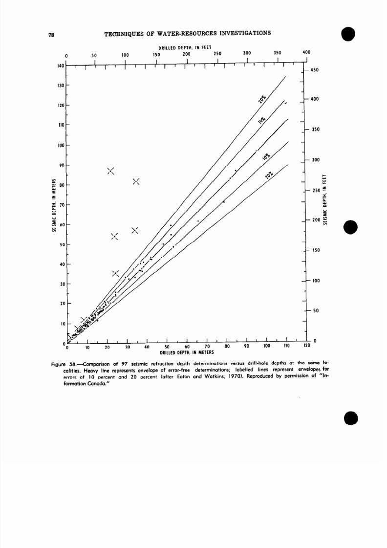
A figure commonly quoted in the literatureconcerning the magnitude of error involvedin seismic refraction depth calculations is 10percent. Eaton and Watkins (1970) appearto substantiate this oft-quoted value with acomparison between seismically predicteddepths and drilled depths at 9’7 drill-hole

sites (fig. 58). It is notable, however, thatthere are 8 points in this plot which represent errors of at least 30 percent and threeof these represent errors in excess of 100percent. Such data do not reflect incompetence on the part of the geophysicists who

published them, rather they represent an at-tempt at intellectual honesty and a willingness to reveal how far off som’e geophysicalpredictions can be. Because there is a general tendency on the part of most investigators to publish only their successful results,the data show n in figure 58 may be regardedas representing a biased sample. It is probable that the average error in most seismicrefraction work is somewhat greater than 10percent.

There are, on the other hand, publishedexamples in which average errors in depth

prediction are as small as 5 percent. The difference between these extremes of 5 and 100percent stems, in part, from the availabilityof independent geologic information or otherkinds of geophysical data. It should be emphasized that the more information of astratigraphic nature the hydrogeologist cangive to the seismologist, the better the seismic interpretations will be. The geophysicist,like the surveyor, benefits from being ableto close on one or more control points in theform of a borehole or well. In the total ab

sence of independen t geologic or geophysicalinformation, the interpretations can be nobetter than the assumptions made concerningprobable conditions below the surface.

Inspection of figure 58 indicates that thosedepth measurements which are in error by30 percent or more are all on the high side;the seismic method overestimated depths tothe refractors. A common cause of over-estimation is illustrated by figure 57H. Ifunrecognized velocity inversions exist in thesection, an overestimate of depth is inevitable. The thickness of the slow layer and the

velocity difference between it and the layerabove determine the magnitude of the error.

0,ther sources of error pertinent to hydro-geologic studies include (1) discontinuousand abrupt lateral variations of velocity, (2)pronounced velocity anisotropy, (3) blind



120 -

110

100 -

90 -

DRILLEDDEPTH, N METERS

Figure 58.--Comparison of 97 seismic refraction depth determinotions versus drill-hole depths ot the same IO-

calities. Heovy line represents envelope of error-free determinations; lobelled lines represent envelopes forerrors of IO percent and 20 percent (after Eaton and Watkins, 1970). Reproduced by permission of “ln-

formation Canada.”

78 TEOHNIQUES OF WATER-RESOURCES INVESTIGATIONS

DRILlED DEPTH, IN FEET0 50 100 150 200 250 300 350 400

140 I,III 11

III II

II

III 11

I‘I’

I( ’

II

120 -

110-

100 -

90 -‘.’J\

‘.’/\

DRILLEDDEPTH,IN METERS

Figure 58.--Comparison of 97 seismic refraction depth determinotions versus drill-hole depths at the same lo

colities. Heovy line represents envelope of error-free determinotions; labelled lines represent envelopes forerrors of IO percent and 20 percent (after Eaton and Watkins, 1970). Reproduced by permission of ’ ‘In-

formation Canada.”




zones, (4) a highly fractured or weatheredbedrock surface, and (5) hydrologically significant interfaces that do not display velocity contrasts large enough for seismic detection.

Applications of SeismicRefraction Measurements

in Hydrogeology

Mapping Buried Channels

The most common use of the seismicmethod in hydrogeology is in the determination of the thickness of sediments whichoverlie essentially non-water-bearing consoli

dated bedrock, The surface of the bedrockmay be plane or irregular, but it is of special hydrologic ‘interest where it occurs inthe form of a channel l’llled with silt, sand,

and gravel. Typical examples include thefluvial sediments of presentday river va lleysand valley-train deposits in old water courses.Models of this type are particularly welladapted for seismic study if there is an appreciable contrast in velocity between the

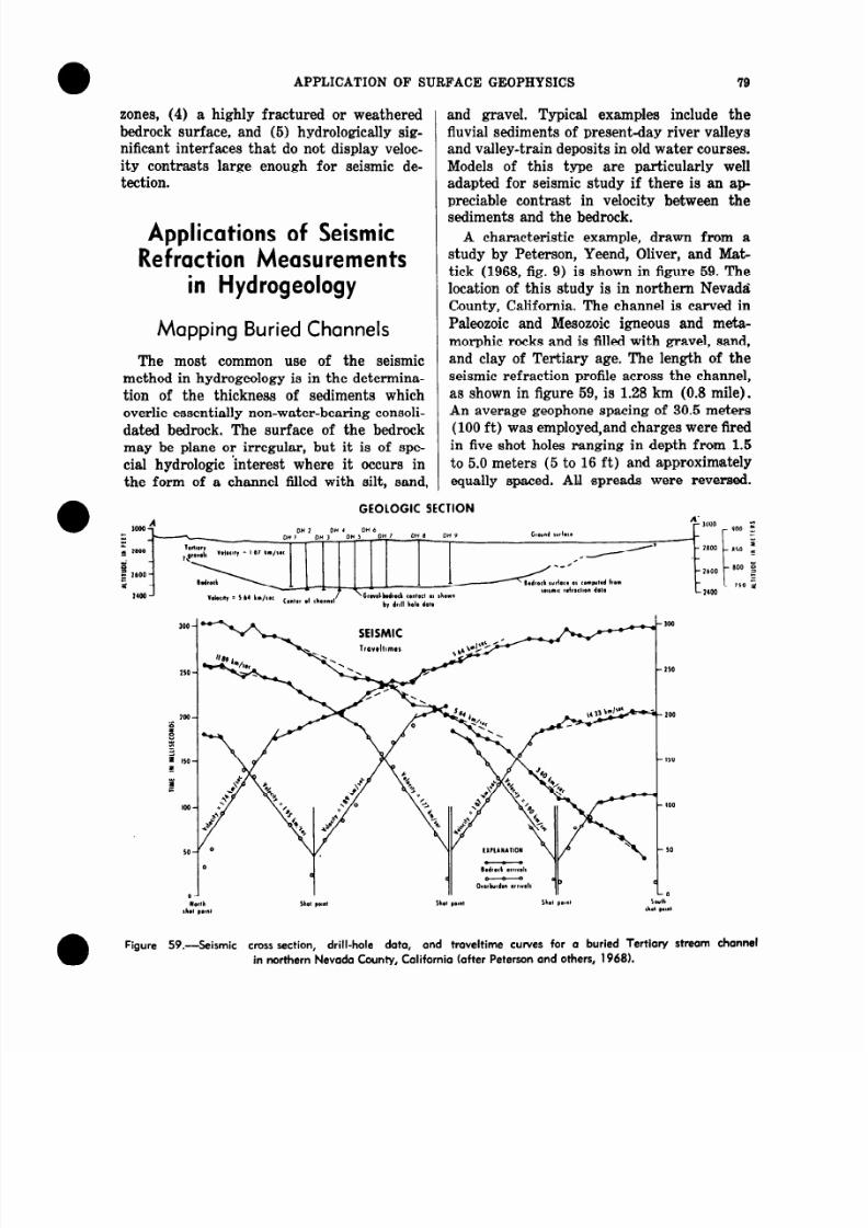
sediments and the bedrock.A characteristic example, drawn from a

study by Peterson, Yeend, Oliver, and Mat-tick (1968, fig. 9) is shown in figure 59. Thelocation of this study is in northern NevadaCounty, California. The channel is carved inPaleozoic and Mesozoic igneous and metamorphic rocks and is filled with gravel, sand,and clay of Tertiary age. The length of theseismic refraction profile across the channel,as shown in figure 59, is 1 .28 km (0.8 mile).An average geophone spacing of 30.5 meters

(100 ft) was employed,and charges were firedin five shot holes ranging in depth from 1.5to 5.0 meters (5 to 16 ft) and approximatelyequally spaced. All ‘spreads were reversed.

GEOLOGIC SECTION

Figure 59.-Seismic cross section, drill-hole data, and traveltime curves for a buried Tertiary stream channel

in northern Nevada County, C alifornia (after Peterson and others, 1968).



80 TECHNIQUES OF WATER-RESOURCES

l-Dynamite charges ‘ranged from 25 to 90 kg

INVESTIGATIONS

each. The elevations of all shot holes andgeophone locations were determined to thenearest 3.0 cm (0.1 ft).

The velocity in the gravel was found fromthe seismic data to average 1.87 km/set (1.16mile/set) and the velocity in the bedrock was5.64 km/set (3.51 mile/set). On the extremenorthern and southern branches of the traveltime curves, apparent velocities in excessof 11 km/set (6.84 mile/set) were recorded.These values are artificial and reflect the factthat the bedrock refractor is dipping towardthe shot point at either end. A schematicmodel of a dipping refractor and its effect onthe traveltime curves was shown in figure57c.

Above the traveltime curves is a geologic

cross section (fig. 69) based entirely on theseismic refraction work. Superimposed on itare vertical lines representing nine drill ho leswhich penetrated to the buried bedrock surface. The correspondence between the twosets of bedrock depths, determined independently, is excellent. The average error incomputed seismic depth for the nine holeswas 4.6 percent and the maximum error, ata single hole, 8.6 percent.

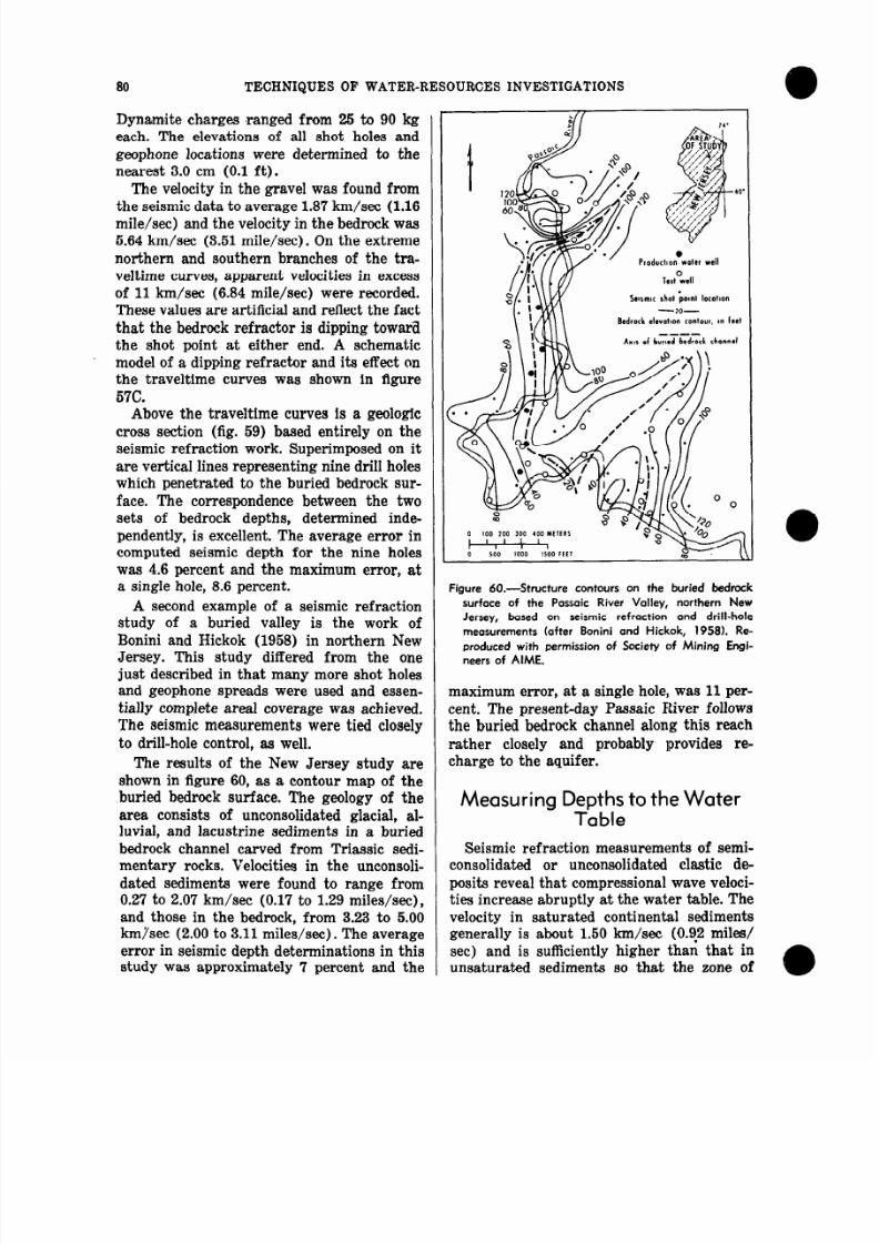
A second example of a seismic refractionstudy of a buried valley is the work ofBonini and Hickok (1958) in northern New

Jersey. This study differed from the onejust described in that many mo re shot holesand geophone spreads were used and essentially complete area1 coverage was achieved.The seismic measurements were tied closelyto drill-hole control, as well.

The results of the New Jersey study areshown in figure 60, as a contour map of theburied bedrock surface. The geology of thearea consists of unconsolidated glacial, alluvial, and lacustrine sediments in a buriedbedrock channel carved from Triassic sedi

mentary rocks. Velocities in the unconsolidated sediments were found to range from0.2’7 to 2.07 km/set (0.17 to 1.29 miles/set),and those in the bedrock, from 3.23 to 5.00kmrsec (2.00 to 3.11 miles/set) . The averageerror in seismic depth determinations in thisstudy was approximately ‘7 percent and the

Figure 60.-Structure contours on the buried bedrock

surface of the Passaic River Valley, northern New

Jersey, based on seism ic refraction and drill-hole

measurem ents (after Bonini and Hick.ok, 1958). Re-

produced with permission of Society of Mining Engineers of AWE.

maximum error, at a single hole, was 11 per-cent. The present-day Passaic Ftiver followsthe buried bedrock channel along this reachrather closely and probably Iprovides re-charge to the aquifer.

Measuring Depths to the WaterTable

Seismic refraction measurements of semi-

consolidated or unconsolidated elastic de-posits reveal that compressional wave velocities increase abruptly at the water table. Thevelocity in saturated con tinental sedimentsgenerally is about 1.50 km/set (0.92 miles/set) and is sufficiently higher than that inunsaturated sediments so that the zone of




saturation acts as a refractor. Observedvelocities in unsaturated sediments generally are less than 1.00 km/see (0.6 miles/see),but rarely may be as high as 1.40 km/see(0.9 miles/set) . According to Levshin(1961) the minimum observed difference in

velocity across the water table occurs in fine-grained sediments a nd exceeds 100 to 150meters/set (330 to 500 ft/sec). In aquiferscomposed primarily of gravel he noted differences as large as 1.00 km/set (0.62 miles/set).

Whether or not the water table can berecognized seismically depends on the thickness of the saturated zone above the bed-rock. In the discussion of figure 5’76, it wasnoted that if the saturated zone is too thinin relation to its depth it will not appear asa separate branch on a traveltime curve pre-

pared from first arrivals only.

Determining the Gross

Stratigraphy of an Aquifer

If some of the velocity discontinuities inunconsolidated or semiconsolidated depositsrepresent stratigraphic breaks in the sedimentary section, seismic refraction measurements can be used, under optimum conditions to unravel the gross stratigraphy of adeposit. If these breaks further represent

SHOT POINT lOCATIONS

0 2 4t 1 I

I I0 I 2 3

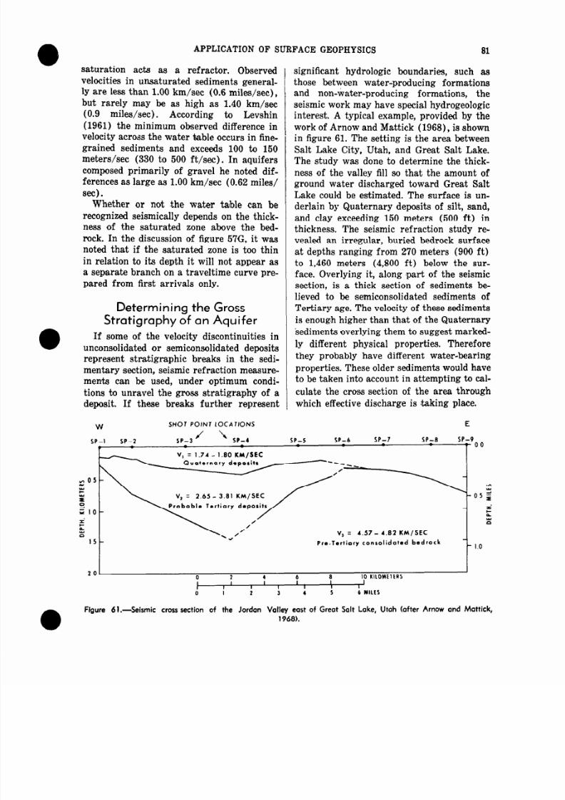
significant hydrologic boundaries, such asthose between water-producing formationsand non-water-producing formations, theseismic work may have special hydrogeologicinterest. A typical example, provided by thework of Arnow and Mattick (1968)) is shown

in figure 61. The setting is the area betweenSalt Lake City, Utah, and Great Salt Lake.The study was done to determine the thickness of the valley fill so that the amount ofground water discharged toward Great Salt

derlain by Quaternary deposits of silt, sand,and clay exceeding 150 meters (500 ft) inthickness. The seismic refraction study revealed an irregular, buried bedrock surfaceat depths ranging from 270 meters (900 ft)to 1,460 meters (4,800 ft) below the sur

face. Overlying it, along ‘part of the seismicsection, is a thick section of sediments believed to be semiconsolidated sediments ofTertiary age. The velocity of these sedimentsis enough higher than that of the Quatornary

sediments overlying them to suggest marked

ly different physical properties. Therefore

they probably have different water-bearing

properties. These older sediments would haveto be taken into ,account in attempting to cal

culate the cross section of the area through

which effective discharge is taking place.

E

V, = 4.5 7- 4 .8 2 KM/SEC

Pro-Tertiary consolidated bedrock - 1.0

b 0 10 KIlOMElERSI 1 I

II 5 6 MILES

Figure 61 .-Seismic cross section of the Jordan Volley eost of Greot Salt Loke, Utoh (after Arnow and Mottick,

1968).




To Hamrlton, Ohlo f

Bedrock wall of valley of ”

ancestral Mlaml River

;y

t//J, To Ohio R iver 0

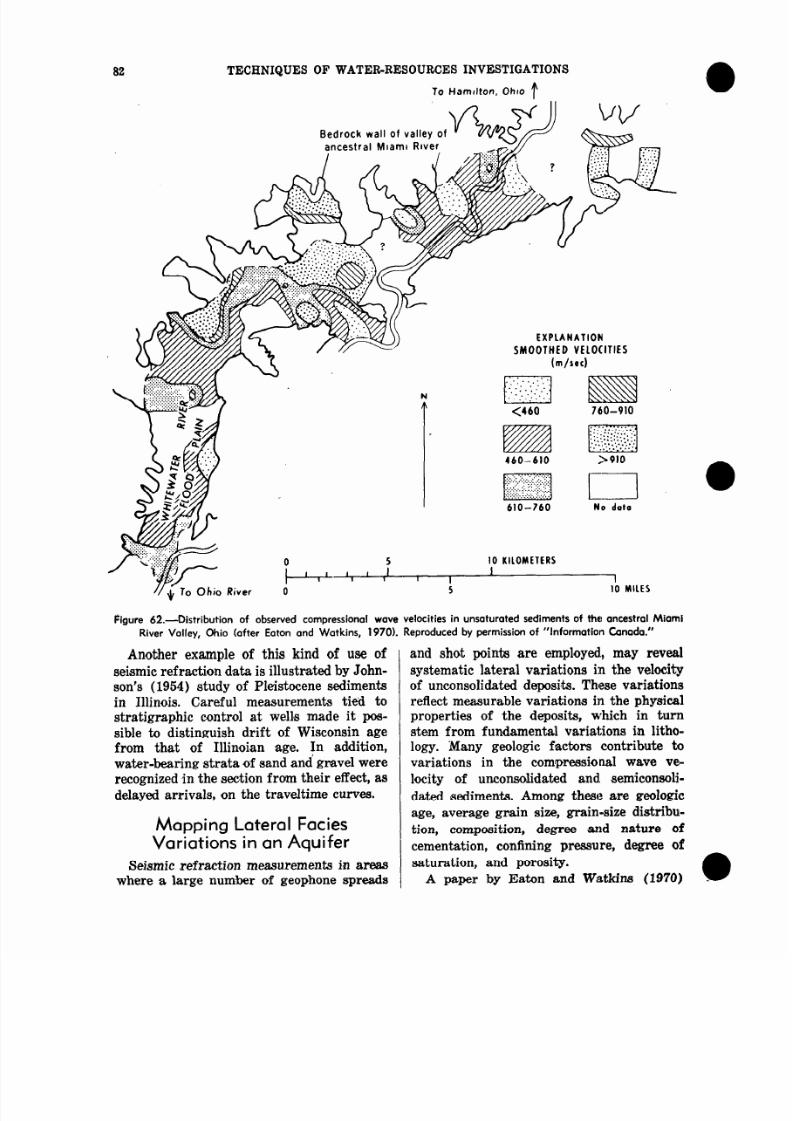
Figure 62.-Distribution of observed compres sional wove

River Valley, Ohio (after Eato n and Watkins, 1970).

Another example of this kind of use ofseismic refraction data is illustrated by John-son’s (1954) study of Pleistocene sedimentsin Illinois. Careful m easurement8 tied tostratigraphic control at wells made it possible to distinguish drift of Wisconsin agefrom that of Illinoian ,age. In addition,water-bearing strata of sand and gravel were

recognized in the section from their effect, asdelayed arrivals, on the traveltime curves.

Mapping Lateral FaciesVariations in an Aquifer

Seismic refraction measurements in areaswhere a large number of geophone spreads

EXPLANATIONSMOOTHED VELOCITIES

(m/se0

460-610 >910

No data

10 KILOMETERS

I II

15 IO MILES

velocities in unsaturated sediments of the ancestral Miami

Reproduced by permission of “Information Canoda.”

and shot points are employed, may revealsystematic lateral variations in the velocityof unconsolidated deposi;ts. These variationsreflect measurable variations in the physicalproperties of the deposits, which in turnstem from fundamental variations in lithology. -Many geologic factors contribute tovariations in the compressional wave ve

locity of unconsolidated and. semiconso lidated sediments. Among these are geologic

age, average grain size, grain-size distribu

tion, composition, degree and nature of

cementation, confining pressure, degree of

saturation, and porosity.A paper by Eaton and Watkins (1970)



APPLICATION OF SURFACE GEOPBYSICS 88

shows the distribution of compressionalwave velocities in unsaturated outwash sandand gravel in the valley of the ancestralMiami River in southwestern Ohio (fig. 62).The velocity variations represent lithofaciesvariations in the upper 30 to 100 meters (100

to 300 ft) of the valley fill. A correlation ofwater wells of high productivity with areasof a given velocity value would allow use ofthe seismic velocity map for locating additional well sites of potential high productivity.

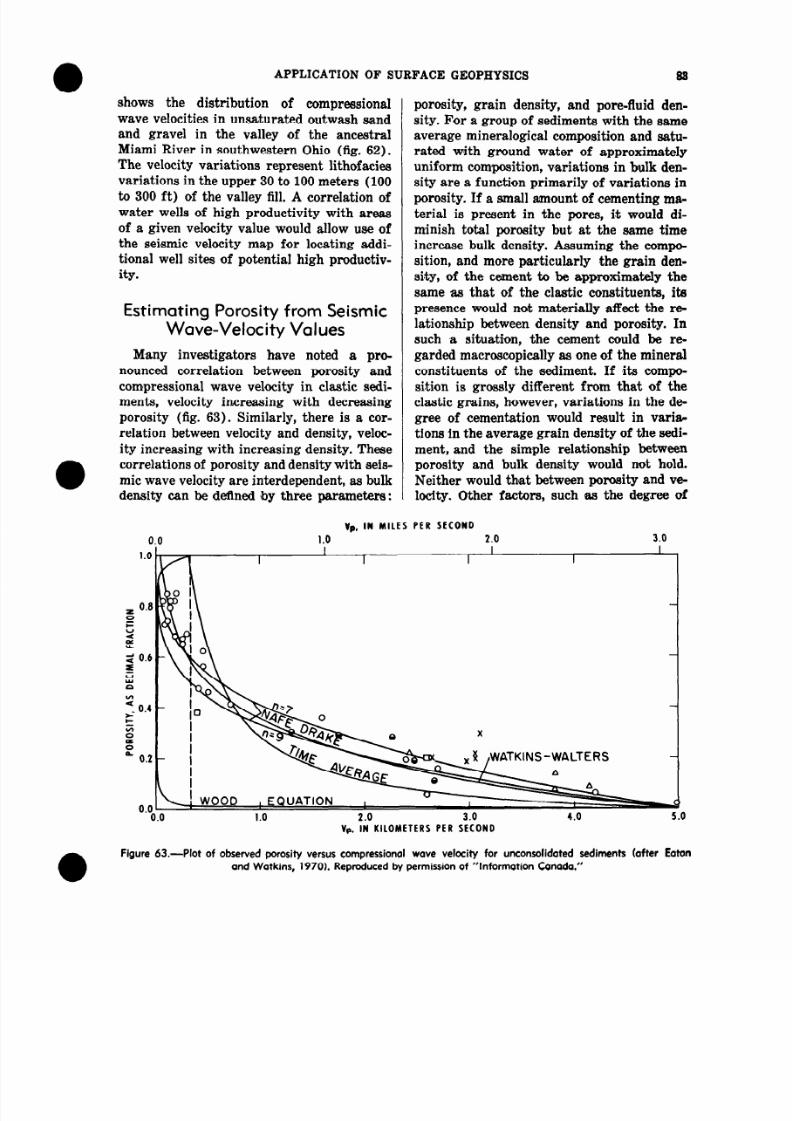
Estimating Porosity from SeismicWave-Velocity Values

Many investigators have noted a pronounced correlation between porosity and

compressional wave velocity in elastic sediments, velocity increasing with decreasingporosity (fig. 63). Similarly, there is a correlation between velocity and density, velocity increasing with increasing density. Thesecorrelations of porosity and density with seismic wave velocity are interdependent, as bulkdensity can be defined Iby three parameters:

VP, IN MILES0.0 1.0

1.0

z 0.8

0CJ

z

< 0.6a=LyCI

2_ 0.4

Eiz

z

20.2

0.00.0 2.0

porosi,ty, grain density, and pore-fluid density. For a group of sedimenti with the sameaverage mineralogical composition and saturated with ground water of approximatelyuniform composition, variations in bulk density are a function primarily of variations in

porosity. If a small amount of cementing material is present in the pores, it would diminish total porosity but at the same timeincrease bulk density. Assuming the composition, and more particularly the grain density, of the cement to be approximately thesame as that of the claetic constituents, it.epresence would not materially affect the relationship between density and porosity. Insuch ,a situation, the cement could be regarded macroscopically as one of the mineralconstituents of the sediment. If ,its compo

sition is gross ly different from that of theelastic grains, however, variations in the degree of cementation would result in variaetions in the average grain density of the sediment, and the simple relationship betweenporosity and bulk density would not hold.Neither would that between porosity and velocity. Other factors, such as the degree of

PER SECOND2.0 3.0

KINS-WALTERS

3.0

VP, IN KILOMETERS PER SECOND

Figure 63 .-Plot of observed porosity versus compres sional wave velocity for unconsolidated sediments (after Eaton

and Watkins, 1970). Reproduced by permissio n of “Information Canada.”



84 TECHNIQUES OF WATERRESOURCES INVESTIGATIONS

fracturing in a semiconsolidated rock, alsoinfluence velocity, the greater the volumedensity of fractures, the lower the velocity.To some extent, however, fractures contribute to the total porosity, so their effect onthe velocity-porosity relationship is not always pronounced. The net result is that velocity values can be used to predict totalaverage porosity, within certain limits, forunconsolidated sediments and weakly consolidated sedimentary rocks.

Experimental data bearing on the systematic relationship between velocity and porosity (fig. 63) in&de rocks and sediments ofa wide variety of compositions. The smoothcurves drawn through the data points areempirically derived m,athematical functionsrelating the two properties. Curves such aa

these could be used in conjunction withmapped velocities like those in figure 62 toproduce maps illustrating area1variations inporosity for uniform sediment.8 in a givenarea. Although the standard deviation ofporosity determined in this way would behigh, the maps might nevertheless serve auseful pume in evaluating the relativewaterstorage potential of the sediments.

References Cited

Arnow, Ted, and Mattick, R. E., 1968, Thickness ofvalley fill in the Jordan Valley east of theGreat Salt Lake, Utah, in Geological Survey

Research 1968: U.S. Geol. Survey Prof. Paper

600-B, p. B’79-B82.

Bonini, W. E., and Hickok, E. A., 1958, Seismic re-

fraction method in ground-water exploration :

Am. Inst. Mining M&all. Engineers Trans.,v. 211, p. 486-488.

Dobrin, M. B., 1966, Introduction to geophysical

prospecting: 2d ed. New York, N. Y., McGraw-

Hill Book, Co., Inc., 446 p.Eaton, G. P., and Watkins, J. S., 1970, The use of

seismic refraction and gravity methods in hy

drogeological investigations, p. 644-668 in

Morley, L. W., ed., Mining and Groundwater

Geophysics, 1967 : Geol. Survey Canada, Economic Geol. Rept. 26, 722 p.

Hawkins, L. V., 1961, The

routine shallow seismic

tions: Geophysics, v. 26,Johnson, R. B., 1964, Use of

method for differentiating

reciprocal method of

refraction investiga

p. 806-819.the refraotion seismic

Pleitiene deposits

in the Arcola and Tuscola quadrangles, Illi

nois: Illinois State Geol. Survey Rept. Inv.

176, 59 p.Kaufmann, H., 1953, Velocity functions in seismic

prospecting: Geophysics, v. 18, p. 289-297.

Levshin, A. L., 1961, Determination of ground-

water level by the seismic method: Akad.

Nauk. SSSR IZU. Ses. Geofiz, no. 9, p. 85%

870.

Peterson, D. W., Yeend, W. E., Oliver, II. W., and

Mattick, R. E., 1968, Tertiary gold-bearing

channel gravel in northern Nevada County,California: U.S. Geol. Survey Circ. 566. 22 p.

Slotnick, M. M., 1959, Lessons in seismic computing: Sot. Exploration Geophysicists, Tulsa,268 p.

Soske, J. L., 1959, The blind zone problem in engi

neering geophysics: Geophysics,, V. 24, p. 359-

365.Willmore, P. L., and Bancroft, A. M., 1966, TL

time term approach to refraction seismology:

Royal Astron. Sot. Geophys. Jour. (London),v. 3, p. 419-432.

Documents

Application of surface geophysics to ground water investigations_C_Sismology.pdf