Claire Imrie and Euan Macrae

DEVEX, May 2014

Application of the ‘Design of

Experiments’ method to estimate

hydrocarbon-in-place volumes

Overview

• Objective of case study was to obtain a range of Hydrocarbon Initially

In Place (HIIP) volumes for a small reservoir, fully accounting for all

identified uncertainties

• i.e. using Design of Experiments to cover the uncertainty space with a

reduced number of geomodels

Workflow:

1. Expert elicitation of uncertain factors,

factor levels and their probabilities

2. A Design of Experiments method

was used to generate an ‘optimal’

dataset, from which a proxy model

could be built

3. The proxy model was then used in a

Monte Carlo analysis to generate a

distribution of possible HIIP volumes

?

I – Relevant theory

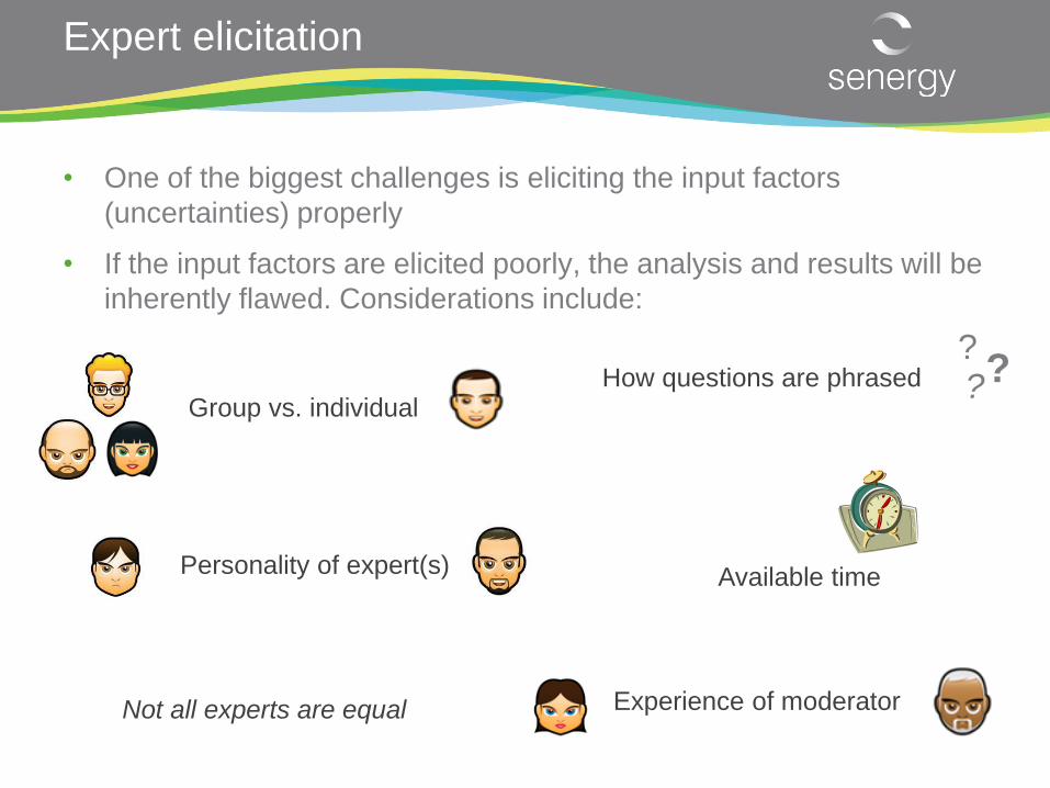
Expert elicitation

Group vs. individual How questions are phrased

Personality of expert(s) Available time

Not all experts are equal Experience of moderator

• One of the biggest challenges is eliciting the input factors

(uncertainties) properly

• If the input factors are elicited poorly, the analysis and results will be

inherently flawed. Considerations include:

? ? ?

• Individual biases (e.g. anchoring, overconfidence, confirmation) and

group biases (e.g. herding) affect us when making judgements

• our intuition can mislead us1,2

• cognitive biases can impact geoscience interpretation3,4

What we did in this study:

• Conducted individual elicitations (one expert per factor)

• Discussed the impact of biases on the experts

• Asked ‘open’ questions and tried to consider alternative explanations

• Talked about assumptions

• Discussed the problem in words and later translated it into probabilities

• Compared experts’ probabilities relatively

1Tversky and Kahneman (1974); 2Capen (1976); 3Baddeley et al. (2004); 4Bentley and Smith (2008)

Expert elicitation (2)

Design of Experiments (DoE) background

• First reference to a designed experiment is from 1747 (reducing the

prevalence of maritime scurvy – James Lind, HMS Salisbury)

• Method first published in 1926 (agriculture) by statistician Sir Ronald

Fisher

Courtesy of Fletcher Bennett (Senergy)

• Advanced during and

after World War II

• Now used in many

science and engineering

disciplines and by the

military

• Used less in oil and gas

industry, but more

common since 2005

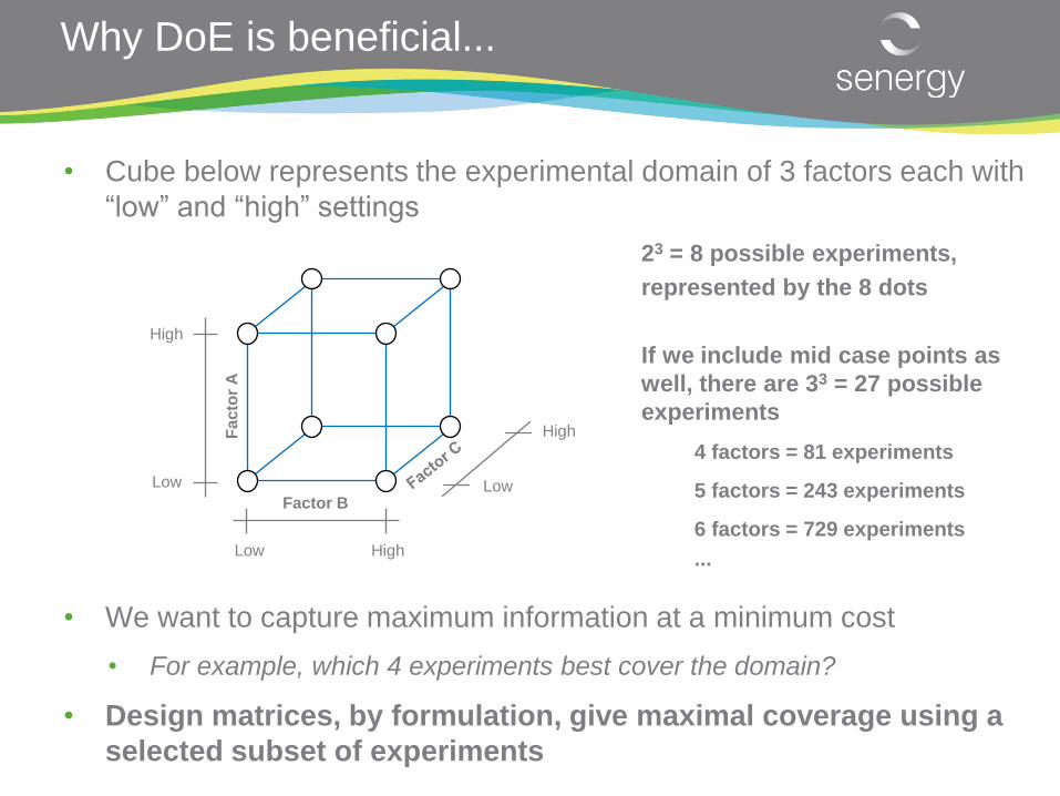
Why DoE is beneficial...

• Cube below represents the experimental domain of 3 factors each with

“low” and “high” settings

• We want to capture maximum information at a minimum cost

• For example, which 4 experiments best cover the domain?

• Design matrices, by formulation, give maximal coverage using a

selected subset of experiments

23 = 8 possible experiments,

represented by the 8 dots

If we include mid case points as

well, there are 33 = 27 possible

experiments

4 factors = 81 experiments

5 factors = 243 experiments

6 factors = 729 experiments

... Low High

Fa

cto

r A

Factor B

Low

High

Low

High

Design matrices

• In experimental design, uncertain factors are varied simultaneously

• this is more robust and efficient than traditional one-factor-at-a-time

analyses

• Below is a 2-level (high and low case) fractional factorial design matrix

(Box et al., 1978)

• we can analyse 9 factors with only 32 experiments – 1/16th of full 29 matrix

http://www.itl.nist.gov/div898/handbook/pri/section3/eqns/2to9m4.txt

• A proxy model is an equation that mathematically represents the

relationship between input variables (e.g. a geomodel) and a

response variable (hydrocarbon volume)

• Monte Carlo (MC) simulations are run on the proxy model using the

factor level probabilities that were originally elicited from the experts

• It is much faster to run the proxy model than the geomodel workflow

• we can complete 10,000 MC runs on the proxy model very quickly

• However, proxy models vary in their ability to represent nonlinearity

and variable dependencies

• the more flexible the model, greater numbers of experiments are

required

Examples:

• Linear

• Polynomial

• Nonlinear methods, e.g. artificial neural networks

Proxy models

Artificial neural networks (ANNs)

• An ANN was used as the proxy

model in this study

• ANNs capture nonlinearity and

account for dependencies

• we have in-house expertise

• adaptive algorithm based on

Fahlman and Lebiere (1989)

• It is a “black box” technique...

• a type of machine-learning

computer model that uses

interconnected and weighted

nodes to empirically solve

numerical problems

• However, it may be hard to

explain to stakeholders

II – The case study

Overview of method

1. Specify problem – choose response variable and

input factors

2. Elicit factor levels and their probabilities

3. Use a ‘screening’ design matrix

4. Analyse screening results with a linear statistical

model

5. Use an ‘optimisation’ design matrix with 3 levels

6. Create proxy model from ~16% of total

experiments

7. Validate proxy model using further 16% of

experiments

8. Use Monte Carlo analysis to predict the range of

HIIP

? ?

?

Introducing the dataset

• A real dataset from a hydrocarbon field

• Field is sealed on one side by a fault and has two reservoir zones:

• a channelised zone

• a relatively homogeneous sandy zone

• There are two wells penetrating the crest of the field

• little well control

• Seismic data are of poor quality

• increased structural uncertainty

• RFT/MDT and fluid saturation data are

ambiguous

• Objective was to estimate the range of

potential HIIP volumes

Uncertain factors

• 9 factors that could impact HIIP were identified via expert elicitation

• Each factor could be varied between low, mid and high values

• Total possible experiments was 39 = 19,683

• A volumetric calculation workflow was built in PetrelTM

-1 0 +1

Top surface deep medium shallow

Separate fault segment? sealing fault some fault degradation no fault

Internal architecture more channelised zone intermediate more homogeneous zone

Channel orientation SW-NE W-E NW-SE

NTG cut-off higher permeability medium lower permeability

Porosity low well log average high

Sand proportion less sand well log proportions more sand

Fluid contacts shallow measured in one well deeper in upper zone

Formation volume factor high latest measurement low

sand proportion

Example factors and their probabilities

less sand

more sand

well log sand

0.15

probability

0.7

0.15

fluid contacts

shallow contact

mid case

deeper contact in

upper zone

0.2

0.2

0.6

probability

Factor screening

F-value (test statistic) Critical value

Results

• ‘Channel orientation’ and

‘FVF’ were removed from

the analysis

• ‘Sand proportion’ seems

to be the most significant

factor

• Design matrix with 2 levels

was used for screening

• Only 32 experiments required

to analyse 9 factors

• A HIIP volume was calculated

for each experiment

• Linear model was fitted to the results to analyse the 9 factors

Optimisation stage

• A 3-level ‘optimisation’ design matrix was created for the 7 factors that

passed the screening stage

• Since the field was small, it was possible to conduct 36 = 729

experiments overnight using the volumetrics workflow

R2 = 0.966

residuals include the effect of the

random seeds used in stochastic

property modelling

Proxy modelling

• 50% of the dataset used to

train ANN

• The other 50% used to

validate model

• Results were excellent

• Method worked almost

exactly as well with 25% of

the data used for ANN

training

Monte Carlo analysis

• 10,000 Monte Carlo (MC) simulations of the ANN proxy model were

run to generate a distribution of HIIP volumes (using the prior

probabilities elicited from the experts)

Results

• The range was wider than

that reported in a previous

study

Potential implications

• Reduction in decision risk

• Specific models can be

selected to pass to RE for

dynamic simulations

III – Conclusions

Conclusions

• The method presented allowed a comprehensive treatment of

uncertainty, accounting for discrete as well as continuous variables

• including: structural uncertainties, errors associated with well log

measurements, and natural variation between the wells

• uncertainty space was adequately covered with the use of 729

experiments from a total of 19,683

• good results were achieved with fewer experiments

• Further work could be focused on

• screening factors more robustly (i.e. accounting for nonlinearity) while

still using a limited number of experiments

• determining the relative impacts of the input factors in a nonlinear and

probabilistic analysis

• selection of models for dynamic simulations

Any questions?

References

Baddeley, M. C., Curtis, A., & Wood, R. (2004). An introduction to prior information derived from

probabilistic judgements: elicitation of knowledge, cognitive bias and herding. Geological Society,

London, Special Publications, 239(1), 15-27.

Bentley, M., and Smith, S., 2008, Scenario-based reservoir modelling: the need for more determinism and

less anchoring, in Robinson, A., Griffiths, P., Price, S., Hegre, J., and Muggeridge, A., eds., The Future

of Geological Modelling in Hydrocarbon Development, Volume 309, Geological Society, London,

Special Publications, p. 145-159.

Box, G. E., Hunter, W. G., & Hunter, J. S. (1978). Statistics for experimenters: an introduction to design,

data analysis, and model building. Wiley-Blackwell, 672 p.

Capen, E. C. (1976). The Difficulty of Assessing Uncertainty (includes associated papers 6422 and 6423

and 6424 and 6425). Journal of Petroleum Technology, 28(08), 843-850.

Fahlman, S. E., & Lebiere, C. (1989). The cascade-correlation learning architecture. Computer Science

Department. Paper 1938.

Tversky, A., & Kahneman, D. (1974). Judgment under uncertainty: Heuristics and biases, Science,

185(4157), 1124-1131.

Thanks are due to our colleagues Steve Spencer,

Patrick Quinn and Hugo Segnini

claire.imrie@senergyworld.com