Embed Size (px)
Citation preview

APPLICATION OF THE GABRIEL GRAPH TO INSTANCE BASED LEARNING ALGORITHMS
Kaustav Mukherjee, B.E (Computer Engineering) University of Pune, 2002
A PROJECT SUBMITTED IN PARTIAL FULFILLMENT OF THE REQUIREMENTS FOR THE DEGREE OF
MASTER OF SCIENCE
In the School
of Computing Science
O Kaustav Mukherjee 2004
SIMON FRASER UNIVERSITY
August 2004
All rights reserved. This work may not be reproduced in whole or in part, by photocopy
or other means, without permission of the author.

APPROVAL
Name:
Degree:
Title of Project:
Kaustav Mukherjee
Master of Science
APPLICATION OF THE GABRIEL GRAPH TO INSTANCE BASED LEARNING ALGORITHMS
Examining Committee:
Prof. Pavol Hell Professor, School of Computing Science, S.F.U Chair
Date DefendedIApproved:
Prof. Binay Bhattacharya Professor, School of Computing Science, S.F.U Senior Supervisor
Prof. Tom Shermer Professor, School of Computing Science, S.F.U Supervisor
Prof. Michael Houle Visiting Professor, National Institute of Informatics, Tokyo, Japan External Examiner

SIMON FRASER UNIVERSITY
PARTIAL COPYRIGHT LICENCE
The author, whose copyright is declared on the title page of this work, has granted to Simon Fraser University the right to lend this thesis, project or extended essay to users of the Simon Fraser University Library, and to make partial or single copies only for such users or in response to a request from the library of any other university, or other educational institution, on its own behalf or for one of its users.
The author has further granted permission to Simon Fraser University to keep or make a digital copy for use in its circulating collection.
The author has further agreed that permission for multiple copying of this work for scholarly purposes may be granted by either the author or the Dean of Graduate Studies.
It is understood that copying or publication of this work for financial gain shall not be allowed without the author's written permission.
Permission for public performance, or limited permission for private scholarly use, of any multimedia materials forming part of this work, may have been granted by the author. This information may be found on the separately catalogued multimedia material and in the signed Partial Copyright Licence.
The original Partial Copyright Licence attesting to these terms, and signed by this author, may be found in the original bound copy of this work, retained in the Simon Fraser University Archive.
W. A. C. Bennett Library Simon Fraser University
Burnaby, BC, Canada

ABSTRACT
Instance based learning (IBL) algorithms attempt to classify a new unseen
instance (test data) based on some "proximal neighbour" rule, i.e. by taking a majority
vote among the class labels of its proximal instances in the training or reference dataset.
The k nearest neighbours (k-NN) are commonly used as the proximal neighbours. We
study the use of the state of the art approximate technique of k-NN search on the best
known IBL algorithms. The results are impressive; substantial speed up in computation
is achieved and on average the accuracy of classification is preserved.
Geometric proximity graphs especially the Gabriel graph (a subgraph of the well
known Delaunay triangulation) provides an elegant algorithmic alternative to k-NN based
IBL algorithms. The main reason for this is that the Gabriel graph preserves the original
nearest neighbour decision boundary between data points of different classes very well.
However computing the Gabriel graph of a dataset in practice is prohibitively expensive.
Extending the idea of approximate k-NN search to approximate Gabriel neighbours
search, it becomes feasible to compute the latter. We thin (reduce) the original reference
dataset by computing its approximate Gabriel graph and use it independently as a
classifier as well as an input to the IBL algorithms. We achieve excellent empirical
results; in terms of classification accuracy, reference set storage reduction and
consequently, query response time. The Gabriel thinning algorithm coupled with the IBL
algorithms consistently outperforms the IBL algorithms used alone, with respect to
storage requirements and maintains similar accuracy levels.
iii

ACKNOWLEDGEMENTS
I would like to take this opportunity to make an attempt to express my gratitude
towards all those people who have played an important role in some way or another to
help me achieve whatever little I have.
First and foremost, I wish to express my sincerest thanks to my Senior
Supervisor Prof. Binay Bhattacharya. This work would not be in the form it is today
without his intellectual inputs and advice throughout the duration of my Master's
program. I am grateful to my external examiner Prof. Michael Houle, on whose work
much of this work is based on. I, to suit my needs, systematically slaughtered his
excellent implementation of the SASH! I am also thankful to Prof. Tom Shermer my
supervisor and the other members of my committee, Prof. Bhattacharya and Prof. Houle
who provided extremely insightful comments into the initial draft of this report. A big
thank you to Prof. Pavol Hell, the graduate director who has motivated the "project
option" at the school, for helping me with the last bureaucratic hurdles.
To my family and especially Mom, my heartfelt thanks for always believing in me
and motivating me to do my best. I feel this a small payback for all that they have
sacrificed for me. Finally, but most importantly, I would like to thank the love of my life,
Bosky to whom this work is dedicated. She is my friend, guide and philosopher and has
been a tower of strength through all my ups and downs for the last five years.

DEDICATION
To Bosky.

TABLE OF CONTENTS
.. ........................................................................................................................ Approval 11
... Abstract ........................................................................................................................ 111
Acknowledgements ...................................................................................................... iv
Dedication ...................................................................................................................... v
Table of Contents ......................................................................................................... vi
... List of Figures ............................................................................................................ VIII
List of Tables ................................................................................................................ ix
List of Abbreviations and Acronyms ........................................................................... x
Chapter 1 Introduction .................................................................................................. 1
.................................................................................................... Motivation 1
Problem Framework .................................................................................... 3
Issues .......................................................................................................... 7
Distance Functions: ..................................................................................... 7 Border and Interior points ............................................................................ 8
Previous Work ......................................................................................... 1 0
........................................................... Instance based learning algorithms 10 ............................................................ Exact k-Nearest Neighbour Search 15
Approximate k-Nearest Neighbour Search (the SASH) .............................. 15 Proximity Graph based methods ................................................................ 16 Support Vector Machines ........................................................................... 21
............................................................................................. Contributions 21
Outline of work ........................................................................................... 22

Chapter 2 Reference Set Thinning With Approximate Proximal Neighbours .......... 24
2.1 The Approximate Gabriel Neighbour Approach .......................................... 24
2.1 . 1 The GSASH ............................................................................................... 24 2.1.2 The Approximate Gabriel Thinning Algorithm ............................................. 35
2.2 The Approximate Nearest Neighbour Approach ......................................... 36
2.3 A Hybrid Approach ..................................................................................... 37
Chapter 3 Experimental Results ................................................................................. 39
3.1 Results on real-world data ......................................................................... 39
3.2 Results on synthetically generated data ..................................................... 43
Chapter 4 Conclusion ................................................................................................. 47
Bibliography ................................................................................................................ 50
vii

LIST OF FIGURES
Figure 1.5: Empty circle property of Gabriel neighbours and good decision
boundary presewati~n------------------------------------------------------------~----- 20
Figure 2.1 : The GSASH structure------------------------------------------------------------------- 28
Figure 3.1 F-shaped boundary results----------------------------------------------------------- -44
Figure 3.2 Circular boundary results------------------------------------------------------------- -45
Figure 3.3 Random rectangular strip boundary results------------------------------------ -46
viii

LIST OF TABLES

LIST OF ABBREVIATIONS AND ACRONYMS
1. GSASH - Gabriel Spatial Approximation Sample Hierarchy.
2. IBL - Instance Based Learning.
3. k-NN - k Nearest Neighbours.
4. NN - Nearest Neighbour.
5. SASH - Spatial Approximation Sample Hierarchy.
6. SVM - Support Vector Machines.
7. UCI - University of California, Irvine.

CHAPTER 1
INTRODUCTION
1 .I Motivation
Recent years have witnessed an explosive growth in the amount of data that is
being generated by corporations, agencies and government as well. Organizing the
large amounts of data make it possible to make better use of this data. This viewpoint
has been recognised and people are now keen on extracting more out of data, i.e.
instead of blindly building large collections of data, the focus has been on recording
observations and then structuring the same. This can be seen as value added data or
quite simply, information.
In several real-world domains, for every observation that is made it is possible to
associate a class membership attribute. For example in an office, every object may be
classified either as being a furniture object or a non-furniture one. So for an observation
of a chair, the class attribute would be "furniture". Let us look at a couple of more
concrete examples.
Its election time. People generally vote based on what issues are important to
them. So voter statistics agencies get busy with gathering information on a
representative sample of the population about relevant election issues. People are

interviewed and their opinions on issues are recorded. Each issue is treated as an
"attribute" for the particular person or observation. Finally they are asked as to what
party they would vote for. Note that the data collection agency may add some attributes
to the recorded observations such as geographical location of the voters etc. So the data
collected about the voters constitutes the observations and the party they vote for
indicates their class membership. Assuming that the observations were made on a
representative sample of the population, we can now generalize these observations to
the entire population, especially the undecided voters (assuming we have their views on
election issues). Therefore the voter statistics agencies can now predict accurate
election results before the actual elections.
"At one time, cancer of the cervix was a major cause of death among women in
British Columbia. However, there has been a major decrease in the death rate because
of screening, early diagnosis and treatment" [BC Cancer Agency]. By recording cell
observations, it can be classified whether the cells are normal or abnormal. If we have
sufficient representative examples of both normal and abnormal observations, we can
quickly and accurately classify new cases, which is what the BC Cancer Agency has
done. By regular screening they have managed to achieve an 85% reduction in the
number of B.C. women getting cancer of the cervix and for reducing cervical cancer
deaths by 75% since the 1950s [BC Cancer Agency].
The above examples should be motivating for computer scientists to develop
accurate and fast "pattern classification" techniques; i.e. using previously recorded
observations, classifying unseen cases. Accuracy is important, as we want our results to
be reliable; speed is important because with so much new as well as old data that can
become irrelevant as time passes, we need to produce results that are relevant to the
time frame in which they were collected. We now embark on our study.

I .2 Problem Framework
Our pattern classification problem can be precisely formulated as follows:
Input: A set of vectors V called the reference dataset. Each reference vector can be
denoted as V, = {Xi, ci}, where is another vector (often called a feature vector,
(Toussaint [I 81)). The feature vector X, is composed of d scalar components or features,
where d is the dimensionality (number of features) of the problem.
= {xi,, xi*, .. . xid}. ci tells us the class label of the feature vector Xi.
Problem: To determine the class label for a new instance 4.
Classical parametric solution:
Bayes decision theory (Duda and Hart [lo]) says that if we know both the a priori
probabilities (the probabilities of certain "classes" of observations or feature vectors) and
the conditional probability densities (the probabilities that certain observations are made
given that we already know the classes of the given observations), then we can compute
the a posteriori probabilities (i.e. the probabilities of given observations being of certain
classes), using Bayes Rule.
So now if we make a new observation Y, all we simply compute is the a posteriori
probabilities using Bayes rule. The a posteriori probability associated with the class ci
that is maximal is chosen and the class ci is the class label attached to the observation.
Thus we can safely say that the Bayes rule does minimize the probability of error
simply because it picks the "most probable" class label for a given observation. In this
sense Bayes rule is optimal. It however makes the (practically unrealistic) assumption
that the distribution of the observationslfeature vectors is known.

Classical non-parametric solution:
The classical non-parametric solution to the pattern classification problem is the
use of the nearest neighbour rule (Cover and Hart 191). (It is a non-parametric technique
as the forms of the underlying probability distribution functions are treated as unknown,
and in practice this is almost always the case.) We have a set of stored instances or
sample points whose class labels are known. We are asked to classify an instance, i.e.
its class label is to be determined. The rule itself is straightforward:
"Classify an instance whose class label is unknown with the same class label as that of its nearest instance in the stored set ".
The problem can be visualized as partitioning the feature space (some metric
space) into regions, where each region ideally consists of observations of a unique class
or category (see figure 1.1 on the next page). As we can see, there is a clear cut
"decision boundary" which separates instances of classes 1 and 2. (The decision
boundary is not necessarily homeomorphic to a line; it could be even be a closed loop)
We can now predict what class a new point would belong to by simply verifying whether
the point lies on the left hand side (class 7) or the right hand side (class 2) of the
decision boundary.

Figure 1 .I Partitioning of attribute space into distinct regions based on class.
CLASS 1 point: 0 CLASS 2 point: fB Decision boundary: ,- - - - I
This seemingly na'ive rule is powerful for two reasons:
1. It is intuitive in the sense that things that have similar properties or attributes are
near to each other spatially. This property is sometimes referred to as "spatial
auto correlation".
2. Perhaps more important is the fact that the error rate of this rule is upper
bounded by twice the (optimal) Bayes error rate (Duda and Hart [lo]) for a large
enough reference dataset. In other words, just this basic proximity information
has at least 50% of the entire information that an optimal classifier would require.
An obvious generalization of this basic rule is the k nearest neighbour rule, which
intuitively means that to classify an unseen sample we take a majority vote of the class
labels of its k closest samples in the stored dataset. The use of this principle has been

shown to obtain good estimations of the Bayes error rate (Toussaint [18]) for large
enough reference datasets. There have also been extensions to the basic rule to reduce
the number of samples stored but still try to obtain the same accuracy as the basic NN
rule (see Hart [ I 21, Gates [ I I]). However the original problems of storage of a huge set
of instances still remain. As a result to compute the nearest neighbour for each point, we
have to look at a large stored dataset. Even incorporating "sophisticated" tree-based
search structures, does not solve the problem of a potentially vast search space in
relatively higher dimensions (Beyer et al [5], Houle [13]). Thus the efficacy of the rule is
limited by its computationally intensive nature. This is why reference set thinning is
essential (Hart [I 21).
Let us call our original reference set V. If the algorithm is decremental in nature (as
ours is), we start with a non-empty set of points V and apply our deletion criterion on
each point. If a point satisfies the criterion, which is basically some boolean condition,
then we remove the point from V. We continue with this step until some stopping
condition is reached. This is also typically a boolean criterion. Our final reduced set is
say, V' that we use for classification of new points. This is the essence of reference set
thinning.

1.3 Issues
1 .XI Distance Functions:
We will focus on two distance functions that we employ for testing all the
algorithms. This consistency is essential as different distance functions can lead to
significantly different accuracy results. For a fairly exhaustive list of distance functions
please look at Wilson and Martinez [20]. One of the distance functions that we use for
datasets with only numeric data is the well known Euclidean distance function:
where is the feature (attribute) vector,
d = number of features (dimensions), Xi= {xil, ~ i 2 , . . ., xid)
When the dataset has non-numeric (nominal) attributes as well, then we use an
alternate distance function called the Vector-Angle metric (Houle [ I 31). It is calculated as
follows:
where X1.X2 is the dot product between the two vectors and I( I( is the norm of the vector'
The distance is some value between 0 and 1 where the value 0 indicates
extreme dissimilarity and the value 1 indicates exact similarity.

1.3.2 Border and Interior points
A very important factor for most Instance Based Learning algorithms is whether
they focus on the retention of the so called border or central points. As we have already
seen in section 1.2, the nearest neighbour decision boundary is an important part of the
feature space, which distinguishes points between different classes. So our focus should
be to keep the decision boundary more or less intact. Intuitively this means that points
closer to the decision boundary are important to maintain the same and these are the
border points. In the corresponding Voronoi diagram (see de Berg et al [4]) of the set of
points, the Voronoi cells, which share a common face with another cell having a point
from a different class, are the border points. The union of these common faces forms the
nearest neighbour decision boundary. So in order to maintain the decision boundary we
should try to keep most border points and thin our reference set by discarding the
interior points that do not contribute to the decision boundary (the unlabeled points in
figure 1.2).

Figure 1.2 Border Points Versus Interior Points
r - - - CLASS 1 point: 0 CLASS 2 point: @ NN Decision boundary: .'
x: CLASS 1 border point y: CLASS 2 border point

1.4 Previous Work
1.4.1 Instance based learning algorithms
Instance based learning (IBL) algorithms (Aha et al [ I ]) are a subset of
algorithms from the machine learning literature which use "instances" (our reference
vectors) from a stored reference set as a means of generalizing the classes of new
unseen instances. As already discussed in section 1.2 and the subsection 1.3.2, these
algorithms are faced with the challenge of finding the "right number" of instances to save
for generalizing. These algorithms generally compute the k nearest neighbours of each
stored instance and use certain relationships to decide whether to keep or throw away
the instance. To compute the nearest neighbour(s), these algorithms use a distance
function (described in subsection 1.3.1) to decide how "close" each instance is to its
neighbours. For an in depth survey of IBL algorithms of the past and their development
through the years Wilson and Martinez [20] and Brighton and Mellish [7] provide good
surveys. Let us now look briefly at the two most powerful and undoubtedly the state of
the art in IBL algorithms.
1.4.1 .I The Decremental Reduction Optimization Procedure 3 (DROP3)
This powerful algorithm was proposed by and first described in Wilson and
Martinez [ I 91 under the name RT3. Basically it computes two sets for each instance; the
k nearest neighbour set and the associate set. The k nearest neighbour set is exactly
what the name suggests, a set of k nearest neighbours of the given instance. The
associate set for a given instance p, consists of a set of those instances A, which have p
as one of their k nearest neighbours. Each instance p also maintains a nearest enemy
e', which is the instance nearest to p (could be a k-NN of p), with a different class than

that of p. The original reference set is denoted by V. The reduced reference set is
denoted by V'. Initially, we have V'= V. The algorithm works on the following rule:
"Remove an instance p if a majority of its associates in V would be correctly classified without p".
Intuitively the above rule means that the algorithm tests for "leave one out cross
validation" generalization accuracy, which is an estimate of the true generalization
capability of the resulting classifier (Wilson and Martinez [20]). An instance is removed if
its removal does not hurt the accuracy of the nearest neighbour classifier based on the
reduced reference set (the set without the instance in it).
There are two somewhat subtle modifications to this basic algorithm.
1. We have already discussed in section 1.3.2, that we need to preserve the border
points and that central points can be removed without any loss of classification
capability. To this end, the DROP3 algorithm sorts all the instances in V' by the
distances to their nearest enemy. It then performs the test of removal of
instances beginning with the instances furthest from their nearest enemies,
thereby testing for central points first (which would have their nearest enemies far
away) rather than border points. This gives the border points a greater chance of
survival.
2. There is the problem with noise in real datasets (i.e. instances that have been
labelled with a different class than its correct class label). To alleviate this,
DROP3 employs what is known as a noise filter before sorting the instances. The
noise filter simply removes those instances that are misclassified by their k
nearest neighbours. This idea was proposed by Wilson [21] and the name Wilson
Editing has been coined for the same. Classifying unseen data using the 1-NN

rule, even with a simple Wilson edited dataset is so powerful that the error rate
converges to the (optimal) Bayes error (Toussaint 1181).
Thus, the algorithm first performs this noise filtering pass, sorts all the instances
with respect to increasing distance from their nearest enemy and then does the removal
test on this sorted list of instances. The final classification or testing step is done by
computing the k-NN for each test case and taking the majority vote among the class
labels of the same. On average, testing with several datasets from the UCI machine
learning data repository, Wilson and Martinez have shown this algorithm to reduce the
reference set size to 15-20% of the original while maintaining the classification accuracy
level of the basic k nearest neighbour classifier which stores 100% of the instances. The
pre-processing or training step requires 0(n2) time in the worst case.
1.4.1.2 The Iterative Case Filtering Algorithm (ICF)
This iterative algorithm was proposed by and described in Brighton and Mellish
[7]. The algorithm is similar to DROP3 in the sense that it also computes nearest
neighbour and associate sets for each instance in the reference set. The key difference
is in the way that these sets are manipulated. Brighton and Mellish call the neighbour
and associate sets as reachable and coverage sets respectively.
One important difference between DROP3 and ICF is in the way the
neighbourhood set of an instance is computed. DROP3 computes this by fixing an upper
bound of k on the size of the neighbourhood set. However ICF computes its reachable
(neighbourhood) set adaptively. Like DROP3 it also maintains a nearest enemy e' for
each instance in the reference set. ICF however uses the nearest enemy to bound its
instance's neighbourhood set; i.e. the set of instances that lie within the hypersphere
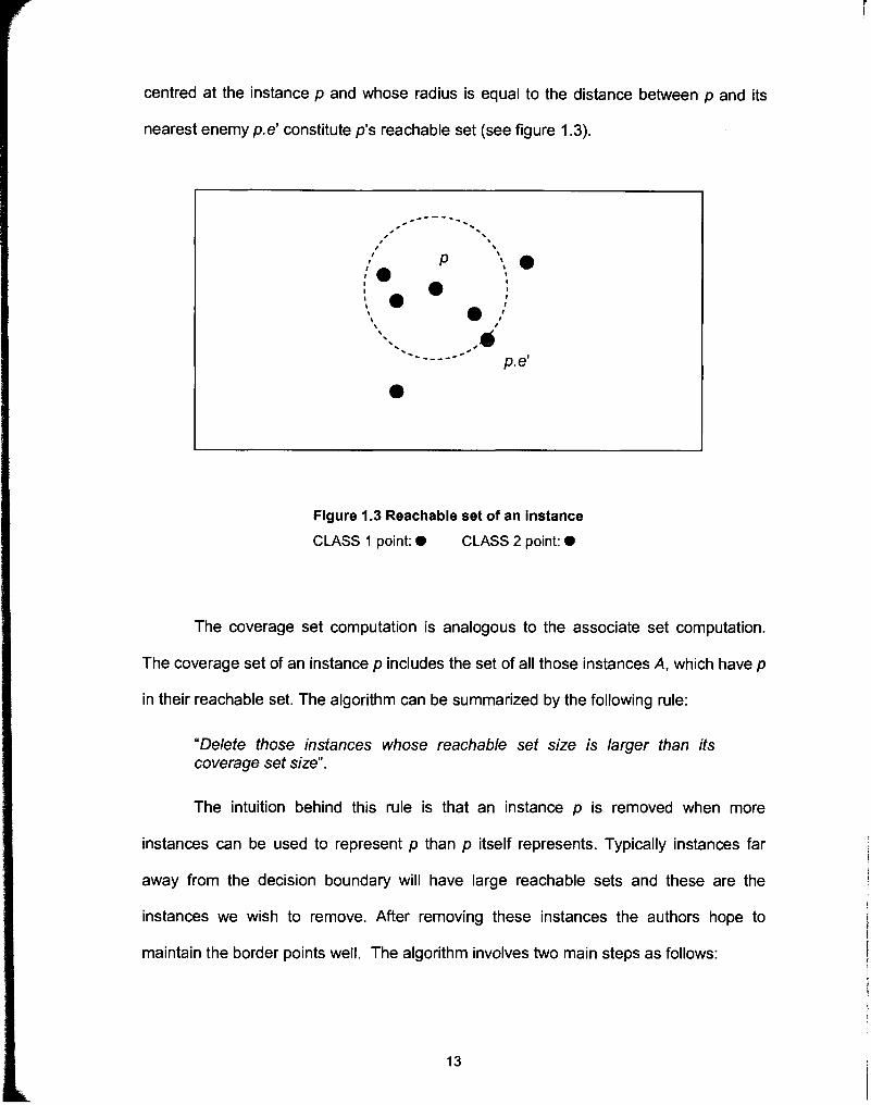
centred at the instance p and whose radius is equal to the distance between p and its
nearest enemy p.e' constitute p's reachable set (see figure 1.3).
Figure 1.3 Reachable set of an instance
CLASS 1 point: 0 CLASS 2 point: @
The coverage set computation is analogous to the associate set computation.
The coverage set of an instance p includes the set of all those instances A, which have p
in their reachable set. The algorithm can be summarized by the following rule:
"Delete those instances whose reachable set size is larger than its coverage set size".
The intuition behind this rule is that an instance p is removed when more
instances can be used to represent p than p itself represents. Typically instances far
away from the decision boundary will have large reachable sets and these are the
instances we wish to remove. After removing these instances the authors hope to
maintain the border points well. The algorithm involves two main steps as follows:

We know that noisy points are harmful for our classification task and
like DROP3 we employ the Wilson editing algorithm to filter out these
points; i.e. remove a point if it is misclassified by its k-NN.
We then apply the deletion criterion mentioned before repeatedly.
Those instances that satisfy the criterion are marked for deletion. At
the end of one pass over the dataset all those instances that are
marked are removed. If we remove at least one instance we repeat
step 2 (recomputing the reachable and coverage sets as we go) until
no instances are removed during any one pass. This turns out to be a
good stopping point for the algorithm.
The final reduced dataset is used for classifying the instances using the k-NN
rule similar to the DROP3 algorithm. Asymptotically the ICF algorithm also has a
quadratic running time in the worst case but in practice it runs much faster than the
DROP3 algorithm. This is because it simply "flags" an instance for deletion and only
removes flagged instances at the end of the current pass unlike the DROP3 algorithm
where if an instance is selected for removal we have to remove it immediately and
update the neighbour lists for the associates of the removed instance with a new
neighbour. Brighton and Mellish [7] perform similar testing as Wilson and Martinez [20]
and observe that the storage requirement is reduced to a similar percentage as that of
DROP3. The classification accuracy is also competitive with DROP3 and the basic
nearest neighbour classifier.

1.4.2 Exact k-Nearest Neighbour Search
One of the oldest and most successful methods for nearest neighbour search
has been proposed in Bentley [3]. The data structure proposed is called the k-d tree, the
k-dimensional tree, where k is the number of dimensions. Theoretically the k-d tree
performs nearest neighbour queries in logarithmic expected time. However, the efficacy
of this and many other similar indexing data structures have been questioned with
respect to the effect known as the curse of dimensionality (Houle [13]). As the
dimensions of the search space increase (for even as small as 10-15 dimensions) linear
search outperforms the "efficient" algorithms proposed on these data structures (Beyer
et al [5]). It has also been suggested recently that exact techniques for nearest
neighbour search are unlikely to improve substantially over sequential search unless the
data itself has some specific underlying distribution, which is extremely rare in practice.
Thus recent research effort has shifted attention to finding powerful approximate
techniques for NN search, which is what we describe next.
1.4.3 Approximate k-Nearest Neighbour Search (the SASH)
We use the most recent work in effective approximate multi dimensional index
structures proposed by Houle [13]. Most of the previous work in this field was based on
the more traditional tree based index structure (e.g. Beckman et al [2]). The idea there
was to assign items to the subtree of their nearest node from a limited set of candidates.
However well this choice is made, some nodes will have nearest neighbours that can be
reached only via paths of great lengths. For more details please see Houle [13]. The
data structure proposed by Houle counters this problem by allowing multiple paths
between nodes. Unlike a tree-based structure, nodes have multiple parents, which result
in only very few nodes whose near neighbours can be reached only via long paths. So in

essence the search space is more "compact". The search recursively locates
approximate nearest neighbours within a large sample of the data and follows links from
these sample neighbours to discover approximate neighbours within the remainder of
the set. A modified version of the data structure, the Spatial Approximation Sample
Hierarchy (SASH) will be described in more detail later as it is an inherent part of our
algorithms. We call the modified version as the GSASH (Gabriel SASH).
1.4.4 Proximity Graph based methods
Construct a graph where each vertex is a data point and it is joined by an edge to
its nearest neighbour. This is the nearest neighbour graph (NNG). The minimum
spanning tree (MST) is also a graph, which captures proximity relationships among its
vertices. The proximity graph we are most interested in for applications to IBL algorithms
is the Gabriel graph (GG). Both the NNG and MST are subgraphs of the GG. The GG
itself is a subgraph of the Delaunay Triangulation, (DT) the dual of the Voronoi diagram.
The Voronoi diagram and correspondingly the DT of a point set capture all the
proximity information about the point set because they represent the original nearest
neighbour boundary as discussed below. Discarding all those points whose Voronoi cell
shares a face with those cells that contain points of the same class as the point under
consideration, we obtain a Voronoi condensed dataset (see Toussaint et al [17]). In
terms of the DT, discard all those vertices of the graph that share an edge with vertices
only from its own class. The NN decision boundary is the union of the common faces of
the Voronoi diagram between Voronoi cell neighbours of different classes.
The decision boundary that is maintained after condensing is the same, as that
would have been maintained even if all points had been kept. The error rate is therefore

also maintained. The condensed set is called a decision boundary consistent subset.
Voronoi condensing does not reduce the number of points to a great extent (Toussaint
[I 71). Also the computational complexity of the Voronoi diagram in higher dimensions is
exponential in the number of dimensions. We need to do some more work. If we are
willing to distort the decision boundary slightly we can do much better. Thus a subset of
the edges of the DT has to be selected. Bhattacharya [6] shows results for two such
subgraphs, the Gabriel graph and the Reduced Neighbourhood graph. S6nchez et al
[15], 1161 also do similar experimentation. It has been acknowledged that the Gabriel
graph based condensing is the best. We now explain the algorithm in more detail, as it is
one of the cornerstones of this work.
1.4.4.1 The Gabriel graph
For a set V of n points (reference vectors) V = @,, p2, . . ., pn}, two points pi and p,
are Gabriel neighbours if
disf(pi, pi) < disf(pj, pk) + d i s f h , pk) V k #i,j .. . . . . . . . . . .. . .. . .. . .. . . . . . . . . 1.1
By joining all pairs of Gabriel neighbours with edges, we obtain the Gabriel
graph. In a geometric sense, two points pi and p, are Gabriel neighbours iff the circle with -
diameter as pi, p, (also called the circle of influence of pi and p,) does not contain any
other point p k E V inside it.
The Gabriel graph can be easily constructed from the Voronoi diagram of the
given point set by joining those pairs of Voronoi neighbours by an edge if the edge
intersects the common face between the Voronoi neighbours. For more details on the
Gabriel graph and its properties please see Bhattacharya [6].

1.4.4.2 The Gabriel thinning algorithm
The brute force approach to compute the Gabriel graph is first described: V = ( p l ,
p2, . . ., pn} is our set of points for which we have to compute the Gabriel graph:
1. For each pair of points (pi, pi), i, j = 1, 2, . . ., n; where i < j:
(i) Perform the following test b'k E V and k # i, j:
if dis?(pi, pj] > dis?(pi, pk) + dis?@i, pk)
then pi and p, are not Gabriel neighbours (go back to step 1).
(ii) pi and pi are marked as Gabriel neighbours.
Step 1 takes 0(n2) operations as there are 0(n2) pairs of points to test. Step 1 (i)
requires O(n) operations, for a fixed d number of dimensions. Therefore the complexity
of the nai've algorithm is 0(n3), i.e. cubic for a constant number of dimensions.
Bhattacharya [6] suggested a heuristic method to compute the Gabriel graph,
which asymptotically still has a cubic complexity in the worst case but observed to be
closer to quadratic at least for small dimensions (d < 5). We describe the algorithm
pictorially (see Bhattacharya [6] for details).
As seen in the figure 1.4 (shown on the next page), when testing q as a possible
Gabriel neighbour of p, any point in the right half space RH (B, p), determined by the line
perpendicular to the line pq i.e. B (p, q), could be rejected as it cannot be a Gabriel
neighbour of p.
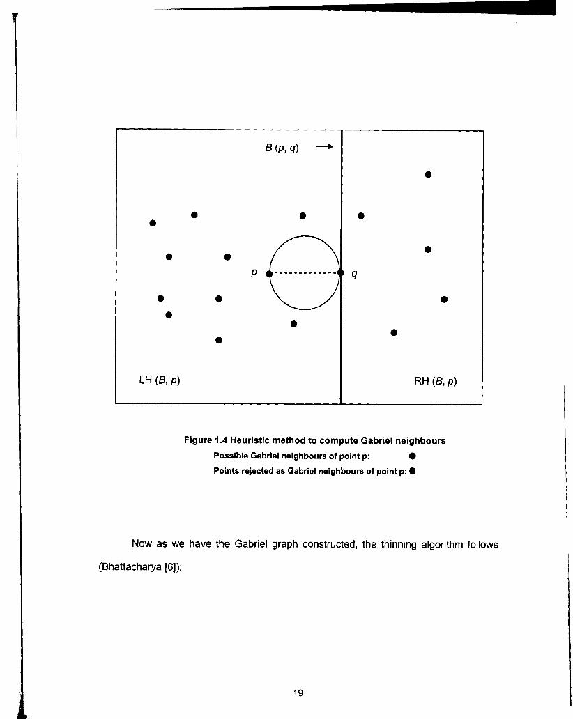
Figure 1.4 Heuristic method to compute Gabriel neighbours
Possible Gabriel neighbours of point p:
Points rejected as Gabriel neighbours of point p: 0
Now as we have the Gabriel graph constructed, the thinning algorithm follows
(Bhattacharya [6]):

Algorithm ExactGabrielThinning:
1. Construct the Gabriel graph of the given set of points.
2. For each point, determine all its Gabriel neighbours. If all the neighbours are
from the same class as the point itself, mark the point under consideration for
deletion.
3. Delete all marked points. The remaining points form the thinned (reduced)
set.
The thinned set generally consists of points located close to the decision
boundary as these points will have as Gabriel neighbours some points on the other set
of the boundary. The boundary itself is slightly "smoothed" (figure 1.5).
Figure 1.5: Empty circle property of Gabriel neighbours and good decision boundary preservation
h--..
CLASS 1 point: 0 CLASS 2 point: @ NN Decision boundary: I' Gabriel decision boundary: r
Point p has Gabriel neighbours from 'other' class and hence is kept. Point 9 does not and hence is removed.

1.4.5 Support Vector Machines
Support vector machines (SVM) (Khuu et al [14]) are a new generation learning
system based on recent advances in statistical learning theory. It is based on the idea of
hyperplane classifiers, or linearly separability of data points. It uses concepts from
integral calculus and quadratic programming to divide the feature space into distinct
separable regions each region for objects of one class.
There are two main disadvantages with this approach (Khuu et al [14]). The
success of an SVM depends heavily on the choice of "kernel functions" which are used
to create the separating decision boundary between the input data. Designing these
functions belongs to a field outside of Computer Science. The second important
drawback is that the performance of SVM declines with increased dimensionality and
reference dataset size.
1.5 Contributions
There are three key contributions that we make in this work:
1. We apply the best-known approximation technique for k-NN search; a spatial
index called the Spatial Approximation Sample Hierarchy abbreviated as the
SASH (Houle [13]) and come up with approximate versions of the state of the
art IBL algorithms that compute the k-NN of the instances or reference
vectors in the stored reference dataset. We preserve the accuracy of
classification with substantial speed up in computation.
2. We next propose a modified version of the SASH to compute approximate
Gabriel neighbours of a set of points in d-space, named the GSASH. It

requires O(n logpn) time and O(n) space to compute the GSASH. The
GSASH can be used to compute the k closest approximate Gabriel
neighbours in O(k logzk + logs n) time.
3. Lastly but perhaps most significantly, we propose a novel Hybrid IBL
algorithm based on the Gabriel proximity graph based thinning and the ICF
algorithm. Experimental results on synthetically generated data and real
world data suggest that the Hybrid algorithm exhibits the best features of its
constituents. It maintains the NN decision boundary faithfully and consistently
outperforms the IBL algorithms used independently for thinning, with respect
to storage (and thus speed).
1.6 Outline of work
The rest of this report proceeds as follows:
Chapter 2 is dedicated to three important sub-parts. In part I, we demonstrate
how we modify the SASH to build the GSASH to compute approximate Gabriel
neighbours. We describe the construction of the GSASH in depth. Then we present
some theoretical upper bounds on the construction and query costs of the GSASH
structure.
Part II explains approximate classifier design using the more traditional k-NN
technique. We show how the IBL algorithms (ICF and DROP3) can be easily modified to
incorporate search for approximate k nearest neighbours using the SASH.
In part Ill, we describe our hybrid two-phase algorithm of reference set thinning

using the Gabriel graph and then further thinning using the ICF algorithm (Brighton and
Mellish 171).
Next, in chapter 3, we perform an extensive experimental comparative evaluation
of the ICF algorithm with the Gabriel algorithm used independently as well as the hybrid
approach described in chapter 2. We perform tests on 14 individual real world datasets
(from the UCI machine learning archive). We also study the behaviour of the different
algorithms in terms of what kind of points they keep by using randomly generated
synthetic data.
We finally conclude in chapter 4 with some observations of our own and suggest
some avenues for further work in this field.

CHAPTER 2
REFERENCE SET THINNING WITH APPROXIMATE PROXIMAL NEIGHBOURS
2.1 The Approximate Gabriel Neighbour Approach
The fundamental point regarding the Gabriel neighbour based approach is that
the Gabriel graph preserves the all important nearest neighbour decision boundary very
faithfully for a given set of points. However as seen before, it is difficult to compute the
Gabriel graph efficiently. So our focus is to compute an approximate version of this
graph sub-quadratically. For this we introduce the GSASH.
2.1.1 The GSASH
The GSASH is basically a modified version of the SASH (the Spatial
Approximation Sample Hierarchy), which is an index structure for supporting
approximate nearest neighbour queries. For more details about the SASH, please see
Houle [I 31. The GSASH (Gabriel SASH) structure is defined next.
2.1 .I .I GSASH structure
A GSASH is basically a graph with following characteristics:
Each node in the graph corresponds to a data item.
Like a tree, it consists of height h E 0(log2n) levels for a dataset of size n. There is
a significant difference here though. For a dataset of size n we actually maintain at

most 2n nodes in the GSASH, with n items at the base or leaf level to a top or root
level with just one node. With the possible exception of the first level, all other
levels have half of the nodes as the level below it. So the structure is as follows:
All the n data items (or pointers to them; we will not make a distinction between
the two in this discussion) are stored at the bottom most level. We then "copy" half
of these i.e. n/2 items uniformly at random to the level above the bottom most. We
repeat this process of "copying" all the way up to the root. At the level just below
the root there are some c nodes (we will discuss the parameter c shortly) and we
pick one of these c to be the root. We will look into this "copying" technique in
more detail in the next section.
Nodes have edges directed to a level above and below except for the root and
leaf levels where edges can only go below and above respectively. Each node
links to at most p parent nodes at the level above and at to at most c child nodes
at the level below it where p and c are constant parameters chosen for
construction. The difference between parent and child edges is purely conceptual,
to illustrate the data structure cleanly. We will have more to say about these
parameters later. The distance dist(a, b) is stored with each edge (a, b).
To ensure that every node is reachable from the root, a parent g is required for
every node v as its guarantor (except for the root itself of course). The child v is
called a dependent of its guarantor g.
2.1 .I .2 GSASH Construction
The edges between the GSASH levels are chosen such that every node is
connected to a small number of its approximate Gabriel neighbours at a level above it.
We can now see the intuition behind the "copying" technique: Each node at level I is

connected to a small number of its approximate Gabriel neighbours among one half of
the nodes from its own level which have been "copied" above at level I - 1. So if a node v
at level I connects to an approximate Gabriel neighbour ra t level I - I it is very likely that
r will be an approximate Gabriel neighbour of v at all levels I' < 1-1 if r is "copied" above.
We now present the GSASH construction algorithm. It is based on the algorithm
ConnectSASHLevel (described in Houle [I 31). Let GSASHidenote the GSASH built up to
level i. The GSASH is built by iteratively constructing GSASHi for 1 I i I h. So our job is
to connect GSASH, and GSASHcl by making parent-child connections between the two.
GSASH, is the root node.
Algorithm BuildGSASH (I):
1. If I = 2, every node in level 2 connects to the root which is the parent for all and the
root has all the nodes in level 2 as its children. The root becomes the sole guarantor
for all its children and the children become the dependents of the root. Thus GSASH2
is constructed.
2. For each node v of level I that we want to connect, do:
(i) For each level I I i < I, pick a set of p approximate Gabriel neighbours Piv) as
follows:
a) If i = 1, then Pi(v) consists of the root.
b) else i > I . C,{v) = the set of distinct children of the nodes in Pi-,(v).
Find the p nearest approximate Gabriel neighbours of v among the nodes in
Ci(v). Use the empty circle property to determine the set of approximate
Gabriel neighbours. Set P,(v) to this set of p closest approximate Gabriel
neighbours. (If less than p neighbours are found at any level i i.e. in C&),
pick all of the available neighbours).

(ii) Set the parents of v to be the nodes of PI-,(v). Each node v is now connected
to p parents, which are its p closest approximate Gabriel neighbours at level i.
3. Create child edges for all nodes of level 1-1 as follows:
a) For each node u of level 1-1, determine the set of nodes from level I that
picked it up as a parent. Call this set H(u).
b) Sort H(u) in increasing order of distances from u.
c) Pick the c closest nodes to u among H(u) as the children of u.
4. For each node v of level I, if it was picked as a child of at least one node u from level
1-1, then the closest node from level 1-1 that picked it becomes the guarantor g(v) of
v. Else v is what is called an orphan node.
5. For each orphan node vat level I, we need to find at least one parent from level 1-1,
which can act as its parentiguarantor. We need to find a guarantor which has less
than its allotted share of children c and which is an approximate Gabriel neighbour of
v. We double the size of the candidate parent set and find a guarantor as follows
(Houle [13]):
b) Compute PI-,(v) as in step 2 but with p = 2p.
c) If we cannot find a node with less than c allotted children as a guarantor of v
then i = i + l and go to step 5.b.
d) Else we pick as the guarantor, the node u, which has less than c children and
closest to v. u adds v to its list of children and v adds u to its (previously
empty) parent list.
End of construction of GSASH,.
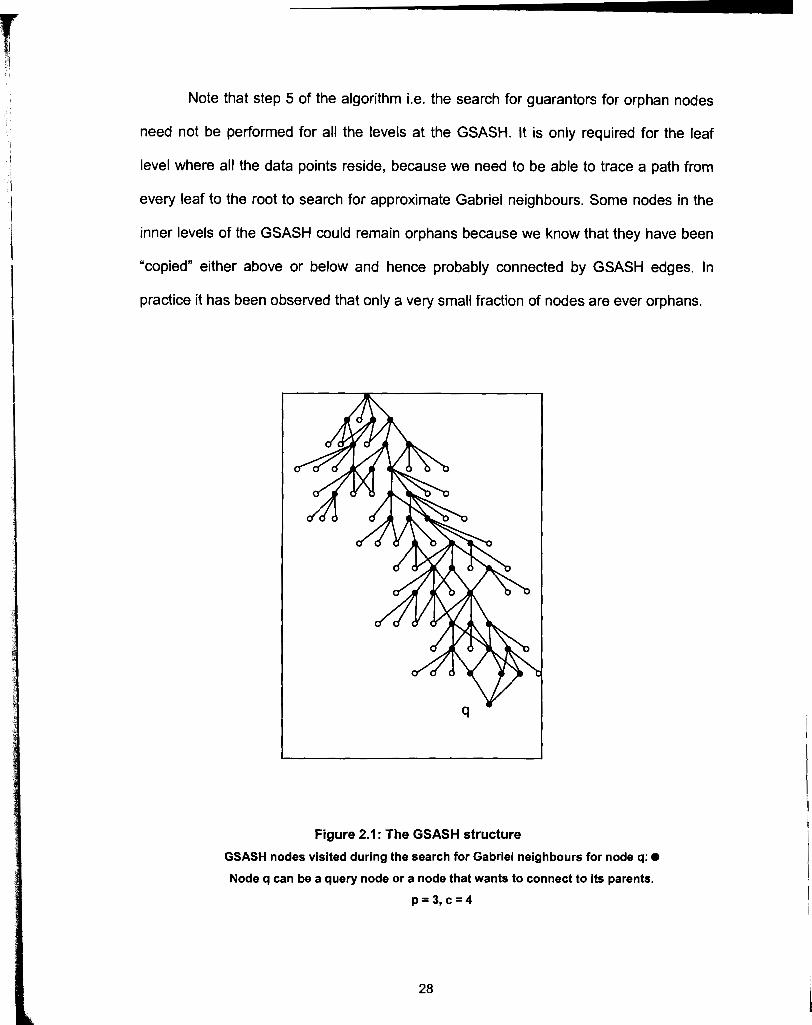
Note that step 5 of the algorithm i.e. the search for guarantors for orphan nodes
need not be performed for all the levels at the GSASH. It is only required for the leaf
level where all the data points reside, because we need to be able to trace a path from
every leaf to the root to search for approximate Gabriel neighbours. Some nodes in the
inner levels of the GSASH could remain orphans because we know that they have been
"copied" either above or below and hence probably connected by GSASH edges. In
practice it has been observed that only a very small fraction of nodes are ever orphans.
Figure 2.1 : The GSASH structure
GSASH nodes visited during the search for Gabriel neighbours for node q: 0
Node q can be a query node or a node that wants to connect to its parents.
p = 3 , c = 4

2.1 .I .3 The empty circle test
The empty circle test to check for Gabriel neighbours (step 2(i)c) of algorithm
BuiIdGSASH is described in more detail. For connecting a node v at level I to its set of p
nearest Gabriel neighbours at level I - ?, we need to test the points in the set Cl{v) (for 2
I i < I ) to determine the p nearest approximate Gabriel neighbours of the points at level i.
For any q E Ci(v), we need to determine whether 9 is a Gabriel neighbour of v. In other
words we need to determine whether the circle of influence of point v and 9 is empty with
respect to the point set at level i, which is GSASHi. However, we only consider the points
of Cl{v) instead of the entire GSASHi (because of our "copying technique") for our empty
circle test.
It can be argued that the Gabriel neighbours found in this manner may not be
"true" Gabriel neighbours because we perform the empty circle test on only ICl{v)l 5 pc
nodes whereas there are at least 2 points at the level i. However if q is a true Gabriel
neighbour of v, our test will also likely say so. It is possible for our test to say that 9 is a
Gabriel neighbour of v even when it is not so. The argument made is that at level I-?,
outside of the pc candidates there is at least one point r, which is actually inside the
circle of influence of v and q (and r P C1{v)). This would actually mean that dist(v, r) <
dist(v, 9) and dist(9, r) < dist(v, 9). If point r had been copied above level I -1 (with
probability 1/2), then it is most likely that r would have been picked up at level I-? and
hence q would not be picked as a parent of p. Even in the case of r not being copied up,
because 9 is picked, it would likely imply that r would also be picked (since dist(v, r) <
dist(v, 9)). Hence it is the case that "true" Gabriel neighbours would be picked as
parents.
To reduce computation we could avoid exhaustively testing all pc pairs of
potential neighbours at each level. We could build a SASH on the pc candidates at each

level. The SASH as we know, can be used for making approximate nearest neighbour
queries. So we build a SASH and test whether any of the approximate nearest
neighbours thus found lies inside the circle of influence of node v and its candidate
parent 9. If any one does lie inside the circle, we terminate the search and declare that v
and 9 are not approximate Gabriel neighbours otherwise we continue the search using
the points (which lie outside the circle) at the next level of the SASH until we reach the
leaf level.
2.1 .I .4 GSASH querying
We now propose the GSASH as a means for computing the k Gabriel neighbours
of a given query item q. The querying algorithm works a lot like the candidate parents
generation step (step 2 of Algorithm BuildGSASH). We can simply compute Ph(q) for p =
k and return the result as Ph(g). Instead of simply picking a constant k neighbours from
each level, a variable number of neighbours kican be picked from each level i. kishould
be smaller for higher levels of the GSASH and larger for the lower levels so that a larger
proportion of the search can be made on the largest number of items (those located
closer to the bottom of the structure) Houle [13], talks about this in context of the SASH
and calls it a "geometric search pattern". The value of ki is given by:
ki = max {k 1-(h-i)bogn 1 1 h PC}.
We now describe the algorithm in more detail.

Algorithm FindApproxGabrielNeighbours (q, k):
1. Pick a set of ki Gabriel neighbours from each level 1s i 5 h as follows:
a. If i = 1, P,{q) consists of a single node, the root.
b. If i > 1, let Ci(q) be the set of distinct children of the nodes in Pi-,(@.
c. If i > 1, let P,{q) be equal to the ki closest Gabriel neighbours from this set
C,{q). Use the empty circle property to determine the set of Gabriel
neighbours. If less than ki neighbours are found in the set, return the entire
set.
Return the k nearest elements from the set Ph(q) as the query result. If this set
contains less than k elements return the entire set.
Thus we can find k approximate Gabriel neighbours of any given query point.
2.1.1.5 Upper bounds
We now present some theoretical upper bounds on the construction and query
costs of the GSASH. Note that in our experiments we assign small constant values to
the parameters p and c.
The GSASH storage turns out to be O(n) because each of the nodes in the
structure is connected to at most p other nodes, leading to a total storage of at most
2np.
Ignoring the costs of finding guarantors for orphan nodes (which in practice
account for a very small proportion of the time taken for construction), the GSASH
construction time can be bounded by O(n lognn). This can be explained as follows: For
each of the O(n) nodes, we visit at most 0(log2n) levels of the GSASH, picking p nodes
at each level and finally connecting level 1-1 and level I with c child edges. The constant
factors hidden inside the asymptotic notation include the costs required to perform the
empty circle test for Gabriel neighbours. For each of the p nodes at a given level we can
perform this test on at most c potential neighbours by exhaustively testing all the O(pc)
pairs, incurring a total cost of at most 0(p2c2) (step 2(i)c of algorithm BuildGSASH). Step
2(ii) contributes an additional factor of O(p) and step 3 another O(cn) in the worst case.
So the observed complexity is close to 0(p2c2n log2n). However using the modification
introduced in section 2.1.1.3, we can avoid testing all pc pairs exhaustively by building a
SASH of the pc nodes at each level to compute approximate nearest neighbours of the
node which has to connect to its p parents and then performing the empty circle test
(eqn (1 .I)) using these approximate NNs. Building a SASH on pc nodes incurs a cost of
O(pc loggc) and querying it to compute approximate NNs incurs an additional
logarithmic factor of 0(log2pc) for each node. Hence the complexity of the GSASH
construction can be bounded by O(pc loggc . n log2n).
The GSASH querying complexity is straightforward. For a given query point, we
need to compute the k Gabriel neighbours. We traverse 0(log2n) levels, picking at most
ki closest Gabriel neighbours at each level from a set of size at most cki at the cost of
c2ki2. The complexity can be bounded by 0(c2k2 log2n). However we can reduce
computation here by following a similar idea as that of the construction algorithm and
also by picking ki closest Gabriel neighbours at each level (using the geometric search
pattern as mentioned in section 2.1.1.4). The cost of a geometric approximate k-NN
query using the SASH is O(k + log2n) (Houle [13]). Therefore, we pick ki closest
approximate Gabriel neighbours at each level by building a SASH on k,c candidates and
perform the empty circle test (equation 1 . I ) using the computed approximate NNs of the
node v which we are to connect with its parents. Since the sum of ki for all i is O(k), the
total cost of building a SASH for all levels is O(kc logzkc) E O(k log2k) for constant c. The
approximate k-NN query cost is subsumed by the SASH construction cost. We perform

the query at most at 0(log2n) levels. Thus the GSASH querying complexity reduces to
O(k log2k + log2n).
Note that all these results are overly conservative as we assume that the children
of a given set of nodes are distinct, which in general is most unlikely. In Houle 1131 it has
been suggested that c = 4p is a good parameter setting. p = 4 and thus c = 16 have
been found to be good parameter values and these are maintained as constants
throughout our experimental analysis of the GSASH. We also maintain k = 32 as a
constant (the actual number of Gabriel neighbours computed varies according to the
dataset but is upper bounded by 32).
Therefore considering p and c as constants the upper bounds on the GSASH
construction and query algorithms can be set at:
O(n log2n) . . . GSASH construction.
0(klog2k + log2n) . . .GSASH query for k approximate Gabriel neighbours.
2.1 .I .6 Comparison with exact Gabriel graph computation
We have already noted in subsection 1.4.4.2 that the computation of the exact
Gabriel graph involves a cubic time complexity. Our algorithm computes an approximate
version of the Gabriel graph. By calling the FindApproxGabrielNeighbours algorithm
repeatedly, for every point in the dataset, we can implicitly compute an approximate
version of the Gabriel graph. So where exactly is the approximation in our algorithm? We
set the number of Gabriel neighbours that a node at a lower level can connect to a level
above it, by p. Our algorithm is basically limited by the number of Gabriel neighbours
every node in the GSASH is allowed to connect to.

It can however be argued that each point in the dataset may look at all possible
O(n) points in the GSASH for finding its Gabriel neighbours and therefore, theoretically
we do not save any computation. However, the GSASH searches for the Gabriel
neighbours through a very compact portion of the search space. So, we find a high
proportion of the true Gabriel neighbours (as much as 90% or more) at speeds of more
than an order of magnitude faster than exact computation. We verify this experimentally
in the following table:
Table 2.1: Comparison of execution costs for the approximate and exact Gabriel neighbour computation* (d = no. of dimensions)
No. of points
500 1000 3000
*Implementation in C++, on a Plll 1.2GHz machine, running the g++ compiler under Linux.
All values are in seconds and indicate CPU time. For the approximate Gabriel
neighbours computation, the cost involves both the building of the GSASH and Gabriel
neighbour querying for every point in the dataset. Of course if the set of points is
previously known, the GSASH could be precomputed and the running time would involve
only the cost of querying the GSASH to find Gabriel neighbours. The data consists of
randomly generated points inside a unit hypercube in two, three, four and five
dimensions.
Approximate Exact d = 2 1.28 3.56 13.78
d = 2 3.6 16.75 201.25
d = 3 2.46 5.75 26.43
d = 3 5.71 27.03 339.46
d=4 2.59 6.5 27.1
d = 4 6.03 29.12 360.81
d = 5 4.34 11.0 47.68
d = 5 9.43 46.82 596.38

2.1.2 The Approximate Gabriel Thinning Algorithm
We are now ready to describe our approximate Gabriel thinning algorithm based
on the GSASH. It is basically a two-pass algorithm with an editing (noise removal) pass
and the final thinning pass. The noise removal pass is based on Wilson Editing (Wilson
[20]) and marks for deletion each point, such that the majority of its Gabriel neighbours
are from a different class as the point itself. This is also called proximity graph based
editing (Sanchez et al [15]).
Algorithm ApproximateGabrielThinning:
1. Construct the GSASH of the given set of points (Algorithm BuildGSASH).
2. For each point in the set:
(i) Compute the given points approximate Gabriel neighbours (Algorithm
FindApproxGabrielNeighbours).
(ii) Mark for removal the point, if a majority of its approximate Gabriel neighbours
have a different class label as the point itself.
3. Delete the marked points from step 2.
4. Compute the approximate Gabriel neighbours of the reduced set.
5. For each point in the reduced set:
Mark for deletion those points, for which all its approximate Gabriel neighbours
are from the same class as the point itself.
6. Delete the marked points from step 5.
7. Return the remaining points. This forms the approximate Gabriel thinned set, which
is used for classifying new points (New points are classified by taking the majority
vote among the class labels of their approximate Gabriel neighbours).
2.2 The Approximate Nearest Neighbour Approach
The original SASH (on which the GSASH is based) was actually intended for
supporting nearest neighbour queries. Structurally the SASH and GSASH are quite
similar. The biggest difference is that the "copying" of nodes technique is not employed
in the SASH. Each SASH node corresponds to a unique object in the dataset and nodes
from one level to another are connected based on a distance-based proximity measure.
Apart from these differences, the construction algorithm is similar (except that the SASH
computes approximate nearest neighbours). The query algorithm differs slightly. In the
SASH it is not just the leaf level where all the data points are. So the result of the k
nearest neighbour query would be the best k nodes taken from all the levels and not just
the bottommost one. Also there can be no orphan nodes allowed at any level because in
the SASH every node is distinct and hence needs to have a path to the root.
So, now we have an efficient SASH based procedure to compute the
approximate k-NN of a given data point. We can therefore modify the existing IBL
algorithms to take advantage of this. As it turned out, modifying the ICF algorithm was
straightforward, as it only marks points for deletion if the deletion criterion is satisfied. At
the end of the entire pass over the dataset, it removes the instances. At this point we
have to rebuild the SASH again and perform another pass over the remaining data (if at
least one point was removed during the current pass). In contrast, the DROP3 algorithm
immediately removes a point if it satisfies the deletion criterion and updates the
neighbourhood and associate lists accordingly. The SASH being a static index cannot
support these dynamic insertion and deletion operations. So we modify the DROP3
algorithm to compute "extra" neighbours before hand. So, as long as the neighbour list of
every point contains the minimum k neighbours we can continue. When the number of

neighbours falls below k, we have to rebuild the SASH again. We observe that 2k
neighbours is a good number of neighbours to maintain at the beginning.
It is observed that the results obtained with exact k-NN and approximate k-NN
search on these state of the art IBL algorithms are very competitive for our real world
datasets both in terms of classification accuracy and storage reduction. We now shift our
focus on the ICF algorithm as we develop our Hybrid algorithm. The main reason for this
is that the ICF algorithm is more "adaptive" (as previously discussed in section 1.4.1.2)
than DROP3. Also, the ICF algorithm can be modified more naturally for use with the
SASH.
2.3 A Hybrid Approach
Our Hybrid algorithm combines the best of both the Gabriel thinning and the ICF
algorithm. It is basically a two-phase algorithm. In phase I, we apply Gabriel thinning. In
phase II, the Gabriel thinned set serves as the input to the ICF algorithm. For more
details about the ICF algorithm please look at Brighton and Mellish [7].
Algorithm Hybrid
1. Perform Algorithm ApproximateGabrielThinning.
2. Use the output of step 1 as the input reference set for Algorithm ICF.
(The Algorithm ICF is described on the next page as outlined in Brighton and Mellish
V1).

Algorithm ICF
1. Repeat steps (i)-(iv):
(i) for all instances i in the reference set T:
a. Compute reachable(0
b. Compute coverage(/]
(ii) progress = false
(iii) for all instances i in the reference set T
if I reachable(/] I > 1 coverage(0 I mark i for deletion
progress = true
(iv) for all instances i in T:
if i is marked for deletion, then remove i from T
2. until not progress.
3. return T.
(Note: the reachable and coverage sets computation is described in sub-section 1.4.1.2)
We run extensive tests on both artificial as well as real world data and present
experimental results in the next chapter.

CHAPTER 3
EXPERIMENTAL RESULTS
Our results are divided into two sections. Section 1 deals with results on real
world data obtained from the UCI machine learning data repository. In section 2 we
present results obtained on artificially generated two-dimensional data to show what kind
of thinned data each algorithm maintains, i.e. whether the decision boundary is indeed
faithfully represented or distorted.
3.1 Results on real-world data
I I Characteristics I
I ionosphere 1 351 1 2 1 34 1 Numeric I
Dataset
abalone balance scale breast cancer - w cell cmc
Iris I 150 I 3 I 4 I Numeric liver - buoa 345 2 6 Numeric . . . - . - - -. - -
spambase I 4601 I 2 1 57 1 Numeric
Numeric
ecoli 336 8 7 Numeric
Data Type
Mixed Numeric Numeric Numeric Mixed
- --
Table 3.1: Nature of the real world datasets used
Dimensions
8 4 10 6 10
No. of instances
41 77 625 699 3000 1473
thyroid voting wine
No' Of
classes 29 3 2 2 3
21 5 435 178
3 2 3
5 16 12
Numeric Boolean Numeric

All of the above datasets (except the cell dataset) have been obtained from the
UCI Machine Learning data repository. The cell data was obtained from the Biomedical
Image Processing Laboratory at McGill University. These datasets appear to be the
universal choice for performing experimental analysis of IBL algorithms (Wilson and
Martinez [20] and Brighton and Mellish [7]).
The table a couple of pages ahead (table 3.2) gives us a measure of the
accuracy of each algorithm i.e. the percentage of test cases correctly classified, and the
percentage of storage maintained (with respect to the original dataset size). The results
are obtained by the so-called 10-fold cross validation technique: Each dataset is divided
into 10 equally sized chunks. 10 experiments are run on these chunks with 9 chunks
used as the reference set and 1 chunk as the test set, changing the test chunk for each
of the 10 runs. This is a similar strategy used by both Brighton and Mellish [7] and
Wilson and Martinez [20].
The Gabriel algorithm is the algorithm, ApproximateGabrielThinning of section
2.1.2. This algorithm produces the best accuracy results but consequently also requires
the highest storage. The ICF algorithm is the one described in Brighton and Mellish [7].
The only difference between the original algorithm and the one used here is that we
have used the technique of approximate NN search described in section 2.2. It should
be noted that the results obtained with exact and approximate NN search are very
competitive. For results of the ICF algorithm with exact NN search please look at
Brighton and Mellish [7]. The Hybrid algorithm is the one discussed in section 2.3; a
combination of the Gabriel and ICF algorithm. As can be seen from the table, this
algorithm strikes the best balance between classification accuracy and storage
reduction.

There are some issues related to the "right" distance function. We used the
Euclidean distance and the Vector Angle distance depending on performance. The
Euclidean distance metric is a good choice for predominantly numeric data whereas the
use of the Vector Angle distance metric is a fairly subjective issue. It did well for some
non-numeric and numeric data as well. The choice of distance function can result in
dramatic changes in results. However this was not our main focus. Our aim was on
maintaining consistency across the test results and hence for each dataset we
maintained the same distance function, for each algorithm. Like Sanchez et al [15], we
vary the parameter k (either picking 1 or 3 depending on performance) used for
classifying instances based on k-NN.
There are a few observations to be made about the table 3.2. The results we
obtain and the ones reported by Brighton and Mellish [7] are similar and fairly consistent.
(Note that we use the SASH for approximate k-NN computation whereas Brighton and
Mellish used exact computation, so there are slight variations for a couple of datasets,
but on average, the results are consistent). The Abalone dataset seems to cause the
worst performance for every algorithm, but this is more due to the nature of the data
itself where class boundaries highly overlap and there are a large number of classes
(29). Apart from the thyroid data, the Hybrid algorithm does at least as well as ICF. Also
we observe that the Hybrid algorithm consistently maintains a smaller subset of the
reference dataset for all the tested datasets.
It is not hard to see why the Hybrid algorithm produces the best results. We know
that the Gabriel algorithm maintains the NN decision boundary very faithfully and this
basically is the first pass of the Hybrid algorithm. So now when we use this thinned
version of the original dataset as an input to ICF (which is the second pass of the Hybrid
algorithm), we thin the boundary even more. Instead of maintaining a very thick band of

boundary points (as the Gabriel algorithm does) we maintain a thinned version of the
most important boundary points. We will see in the next section as to exactly what kind
of points do each of these algorithms maintain where the algorithms are compared for
performance on the artificially generated datasets.
Dataset I Hybrid I ICF I Gabriel
Accuracy Storage Accuracy Storage
20.83% 4.20% 23.52% 19.44%
86.78% 11.69% 82.09% 20.96%
95.0% 2.70% 94.88% 3.16%
Accuracy I Storage
abalone
balancescale
breastcancer - w
cell
cmc
diabetes - pima
ecoli
ionosphere
iris
liver - bupa
spam base
thyroid
voting
wine
Table 3.2 Results on real-world data
42

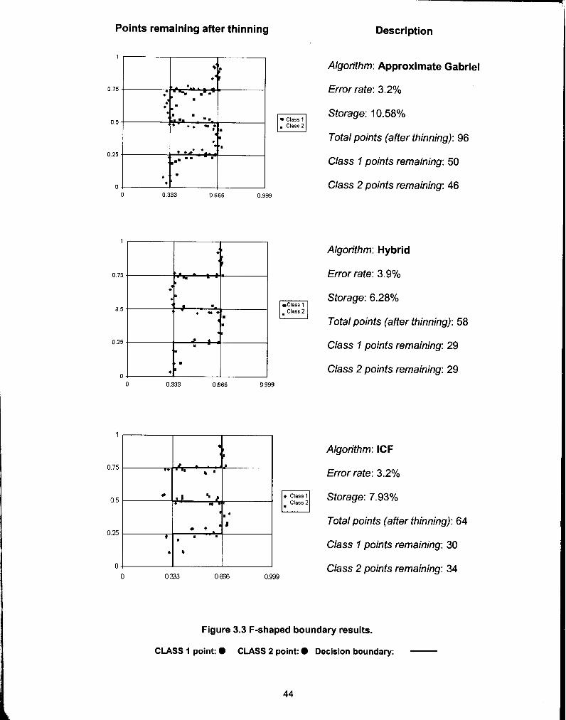
3.2 Results on synthetically generated data
We test our algorithms on three synthetically generated datasets with sharp
regular shaped decision boundaries. All the data is generated inside a unit square and
the decision boundaries are varied. The decision boundaries are F-shaped, circular and
a rectangular strip. Points generated randomly on either side of the boundary are given
opposite class labels. Points inside the boundary are given random class labels.
The data generated is two-dimensional for convenient visualization purposes. We
generate 1000 points randomly. The results obtained are 10-fold cross validated like the
real-world data. The tables shown on the next three pages (tables 3.3, 3.4 and 3.5) show
the points that are kept by each algorithm after thinning. They also show the error rate
and storage reduction percentage for each algorithm, on each dataset (the datasets are
essentially the same in terms of the co-ordinates but the class labels of the data points
vary according to the decision boundaries).
As expected, the Gabriel algorithm produces the thinned subset of points that
tightly maintain the decision boundary at the cost of slightly extra storage. The ICF
algorithm distorts the boundaries significantly, as can be seen in results on the F-shaped
and circular boundaries. There are a significant number of "non-border" points that are
maintained which are not close enough to the boundary so as to classify border points
correctly. This is a significant drawback and this is where the Hybrid algorithm wins out.
Not only does it reduce storage appreciably but also it maintains the decision boundary
quite faithfully. Based on the experimental results, we can say it combines the best of
both worlds: faithful decision boundary preservation a la the Gabriel algorithm and
aggressive storage reduction due to effect of the ICF algorithm.
Points remaining after thinning Description
Class 1
Algorithm: Approximate Gabriel
Error rate: 3.2%
Storage: 1 0.58%
Total points (after thinning): 96
Class I points remaining: 50
Class 2 points remaining: 46
1
Algorithm: Hybrid
o 75 Error rate: 3.9%
Class 1 Storage: 6.28%
0.5 . Class 2 [7 Total points (after thinning): 58
o 25 Class I points remaining: 29
0 Class 2 points remaining: 29
0 0.333 0.666 0.999
Algorithm: ICF
0.75 Error rate: 3.2%
0.5 Storage: 7.93% P - * 4 Class 2
Total points (after thinning): 64 0.25
Class 1 points remaining: 30
Class 2 points remaining: 34
Figure 3.3 F-shaped boundary results.
CLASS 1 point: 0 CLASS 2 point: 0 Decision boundary: -

Points remaining after thinning Description
Class 1 . Class 2 U
Class 1 Fl
Algorithm: Approximate Gabriel
Error rate: 2.5%
Storage: 12.94%
Total points (after thinning): 1 17
Class 1 points remaining: 57
Class 2 points remaining: 50
Algorithm: Hybrid
Error rate: 2.8%
Storage: 7.3%
Total points (after thinning): 72
Class 1 points remaining: 34
Class 2 points remaining: 38
Algorithm: ICF
Error rate: 4.3%
Storage: 7.72%
Total points (after thinning): 77
Class 1 points remaining: 32
Class 2 points remaining: 45
Figure 3.4 Circular boundary results.
CLASS 1 point: 0 CLASS 2 point: @ Decision boundary: 0

Points remaining after thinning Description
Algorithm: Approximate Gabriel
Error rate: 10.4%
Storage: 13.6%
Total points (after thinning): 124
Class 1 points remaining: 59
Class 2 points remaining: 65
Class 2
Algorithm: Hybrid
Error rate: 10.3%
Storage: 8.65%
Total points (after thinning): 75
Class I points remaining: 35
Class 2 points remaining: 40
Class 1 1-q
Algorithm: ICF
Error rate: 1 1.8%
Storage: 6.47%
Total points (after thinning): 50
Class I points remaining: 25
Class 2 points remaining: 25
Figure 3.5 Random rectangular strip boundary results.
CLASS I point: CLASS 2 point: @ Decision boundary: I I

CHAPTER 4
CONCLUSION
In this work, we examine the problem of reference set thinning, also called
training set storage reduction, for instance based learning algorithms. We review the
existing techniques and argue that the state of the art solutions to the problem involve
the heavy computational burden of computing the k nearest neighbours of every
instance in the reference set. lncorporating the use of the SASH, an efficient index
structure for supporting approximate nearest neighbour queries, we find that the existing
techniques can be sped up by substantially with no degradation in classification
accuracy as well as storage reduction.
The Gabriel graph has been long known to be an excellent geometrical construct
to capture proximity relationships between its nodes. However computing it was
practically infeasible because of the worst case cubic time complexity involved.
Incorporating the idea of approximate k nearest neighbour search into approximate
Gabriel neighbour search, we come up with a modified version of the SASH that we call
the GSASH. The GSASH can be constructed in O(n lognn) time for a dataset of size n
and used as a means for computing k approximate Gabriel neighbours of a query point
in O(k logzk + log2n) time We apply the GSASH to compute approximate Gabriel
neighbours and use it in the Gabriel graph based reference set thinning algorithm
proposed by Bhattacharya [6]. The single most important property of the Gabriel graph is
that it preserves the nearest neighbour decision boundary very faithfully. We show

experimental results comparing this algorithm with the best known IBL algorithms and
not surprisingly it turns out the Gabriel thinning algorithm performs better on real world
and synthetic data. The Gabriel thinning algorithm's running time is basically dominated
by the time required to compute the Gabriel neighbours of the reference data set. Hence
the complexity of the algorithm is O(kn log2k + nlog2n).
The only major drawback with the Gabriel thinning algorithm is that it does not
produce a considerable storage reduction compared to the IBL algorithms. This is a
serious issue because of the large amount of data available; computation time
performance can degrade if we maintain a very large subset of the data for pattern
classification. Therefore we propose a hybrid reference set thinning algorithm, which
involves the Gabriel thinning algorithm as the first pass and the ICF algorithm of Brighton
and Mellish [7] as the second pass. Our choice of the ICF algorithm was purely
motivated by the fact that like the Gabriel algorithm it is also adaptive in nature and can
incorporate the SASH quite seamlessly. Our Hybrid algorithm is shown to exhibit the
best features of both of its constituents. It still maintains the decision boundary quite
faithfully and also results in aggressive storage reduction. In fact, its accuracy is
competitive with that of the Gabriel algorithm and its storage reduction surpasses that of
the ICF algorithm.
There is still much work that has to be done especially with approximate proximal
neighbours search. For one, we need to develop dynamic versions of the
SASHIGSASH, which can support insertionsldeletions dynamically without having to
rebuild the structure from scratch. This would save significant computation time.
Our Hybrid algorithm seems to be in line with the cutting edge research in pattern
classification, which suggests the use of "Classifier Ensembles", collections of classifiers
working together. Certain classifiers are good for certain domains while not so good for

others. We believe that a Gabriel neighbour based classifier would be an excellent
addition to these "Classifier Ensembles" simply because of the nature of the Gabriel
graph that preserves the all important nearest neighbour decision boundary very well.

BIBLIOGRAPHY
[ l ] D.W. Aha, D. Kibler & M.K. Albert (1991), Instance-Based Learning Algorithms,,
Machine Learning, 6: 37 -- 66.
[2] N. Beckmann, H. Kriegel, R. Schneider, and B. Seeger [1990]. The R* tree: An
efficient and robust access method for points and rectangles, Proceedings of ACM
SIGMOD Conference on Management of Data, 322 - 331.
[3] J. L. Bentley (1975). Multidimensional binary search trees used for associative
searching. Communications of the ACM, 18(9): 509 -- 517.
[4] M. de Berg, 0. Schwarzkopf M. van Kreveld, and M. Overmars (2000) Computational
Geometry: Algorithms and Applications, Second Edition, Springer-Verlag.
[5] K. Beyer, J. Goldstein, R. Ramakrishnan and U. Shaft (1999). When is nearest
neighbour meaningful? Proceedings of the 7th International Conference on Database
Theory (ICDT), 217 - 235.
[6] B.K. Bhattacharya (1982). Application of Computational Geometry to Pattern
Recognition Problems, PhD Thesis. Simon Fraser University, School of Computing
Science Technical Report TR 82-3,259 pages.
[7] H. Brighton and C. Mellish (2002). Advances in Instance Selection for Instance-
Based Learning Algorithms. Data Mining and Knowledge Discovery, 6: 153 - 172.
[8] T.H. Cormen, C.E. Leiserson, R.L. Rivest, C. Stein (2001). Introduction to algorithms,
Second Edition, The MIT Press.

[9] T. M. Cover & P. E. Hart (1967). Nearest neighbor pattern classification. Institute of
Electrical and Electronics Engineers Transactions on lnformation Theory, 13(1), 21-
27.
[ lo] R. Duda and P. Hart (1973). Pattern Classification and Scene Analysis. Wiley-
lnterscience publication.
[ I l l W. Gates (1972), The reduced nearest neighbour rule, IEEE Transactions on
lnformation Theory, 18: 431 -- 433.
[I21 P.E. Hart (1968), The condensed nearest neighbour rule, IEEE Transactions on
lnformation Theory, 14(3), 51 5 -- 51 6.
[I31 M. Houle (2003). SASH: a Spatial Approximation Sample Hierarchy for Similarity
Search. IBM Tokyo Research Laboratory Report RT-0517, 16 pages.
[I41 H.V. Khuu, H.K. Lee, and J.L. Tsai Machine Learning with Neural Networks and
Support Vector Machines. University of Wisconsin-Madison (Web link: http://
www.cs.wisc.edu/-hiep/Sources/Articles/svms nns research.pdf (date: August 29,
2004))
[I51 J.S. Sanchez, F. Pla, F.J. Ferri (1997). Prototype selection for the nearest
neighbour rule through proximity graphs. Pattern Recognition Letters, 18: 507 -
51 3.
[I61 J.S. Sanchez, F. Pla, F.J. Ferri (1997). On the use of neighbourhood-based non-
parametric classifiers, Pattern Recognition Letters, 18: 1 179 - 1 186.
[I71 G.T. Toussaint, B.K. Bhattacharya and R.S. Poulsen (1984), The application of
Voronoi diagrams to non-parametric decision rules, Proceedings of the 16'~
Symposium on Computer Science and Statistics, 97 --I 08.

[I81 G. T. Toussaint (2002). Proximity graphs for nearest neighbour decision rules:
recent progress, Interface-2002, 34th Symposium on Computing and Statistics
(theme: Geoscience and Remote Sensing).
[I91 D. R. Wilson & T. R. Martinez (1997). Instance pruning techniques. In Fisher, D.
(Ed.), Machine Learning: Proceedings of the Fourteenth International Conference
(ICML197), 403 - 41 1.
[20] D. R. Wilson & T. R. Martinez (2000). Reduction Techniques for instance based
learning algorithms. Machine Learning, 38: 257 - 286.
[21] D.L. Wilson (1972). Asymptotic properties of nearest neighbour rules using
edited data. IEEE Transactions on Systems, Man and Cybernetics, 2: 408-421.