This article was downloaded by: [Hebrew University]On: 16 October 2014, At: 02:19Publisher: Taylor & FrancisInforma Ltd Registered in England and Wales Registered Number: 1072954 Registered office: Mortimer House,37-41 Mortimer Street, London W1T 3JH, UK

Communications in Statistics - Simulation andComputationPublication details, including instructions for authors and subscription information:http://www.tandfonline.com/loi/lssp20

Application of the Generalized Likelihood Ratio Test forDetecting Changes in the Mean of Multivariate GARCHProcessesOlha Bodnar aa Department of Statistics , European University Viadrina , Frankfurt , GermanyPublished online: 24 Feb 2009.

To cite this article: Olha Bodnar (2009) Application of the Generalized Likelihood Ratio Test for Detecting Changes in theMean of Multivariate GARCH Processes, Communications in Statistics - Simulation and Computation, 38:5, 919-938, DOI:10.1080/03610910802691861

To link to this article: http://dx.doi.org/10.1080/03610910802691861

PLEASE SCROLL DOWN FOR ARTICLE

Taylor & Francis makes every effort to ensure the accuracy of all the information (the “Content”) containedin the publications on our platform. However, Taylor & Francis, our agents, and our licensors make norepresentations or warranties whatsoever as to the accuracy, completeness, or suitability for any purpose of theContent. Any opinions and views expressed in this publication are the opinions and views of the authors, andare not the views of or endorsed by Taylor & Francis. The accuracy of the Content should not be relied upon andshould be independently verified with primary sources of information. Taylor and Francis shall not be liable forany losses, actions, claims, proceedings, demands, costs, expenses, damages, and other liabilities whatsoeveror howsoever caused arising directly or indirectly in connection with, in relation to or arising out of the use ofthe Content.

This article may be used for research, teaching, and private study purposes. Any substantial or systematicreproduction, redistribution, reselling, loan, sub-licensing, systematic supply, or distribution in anyform to anyone is expressly forbidden. Terms & Conditions of access and use can be found at http://www.tandfonline.com/page/terms-and-conditions

Communications in Statistics—Simulation and Computation®, 38: 919–938, 2009Copyright © Taylor & Francis Group, LLCISSN: 0361-0918 print/1532-4141 onlineDOI: 10.1080/03610910802691861

Application of the Generalized LikelihoodRatio Test for Detecting Changes in theMean

ofMultivariate GARCHProcesses

OLHA BODNAR

Department of Statistics, European University Viadrina,Frankfurt, Germany

We derive several multivariate control charts to monitor the mean vector of multi-variate GARCH processes under the presence of changes, by means of maximizingthe generalized likelihood ratio. This presentation is rounded up by a comparativeperformance study based on extensive Monte Carlo simulations. An empiricalillustration shows how the obtained results can be applied to real data.

Keywords Generalized likelihood ratio test; Multivariate control charts;Multivariate GARCH processes; Statistical process control.

Mathematics Subject Classification 62L10; 62M10.

1. Introduction

Engle (1982) invented a new method of modeling the volatility of financial timeseries which is based on the recursive calculation of the conditional variance.The structure of the autoregressive process was applied in order to forecast thefuture values of the conditional volatility. The model was extended by Bollerslev(1986) by using the autoregressive moving average process in the conditionalvariance equation. Later on, different univariate GARCH processes were suggestedin the literature. Nelson (1991) proposed the exponential GARCH process tomodel the asymmetry of the returns. The other asymmetric GARCH processes werederived by Engle and Ng (1993), Zakoian (1994), among others.

The extension of the univariate GARCH model to the multivariate case isnot straightforward. As a result several models are suggested in the literature.The first multivariate GARCH model was derived by Bollerslev et al. (1988), whichis based on the VEC representation of the conditional variance equation. Althoughthe model is quite general, it possesses some difficulties in the practical application.

Received July 30, 2008; Accepted December 15, 2008Address correspondence to Olha Bodnar, Department of Statistics, European University

Viadrina, P.O. Box 1786, 15207 Frankfurt (Oder), Germany; E-mail: obodnar@euv-frankfurt-o.de

919

Dow

nloa

ded

by [

Heb

rew

Uni

vers

ity]

at 0

2:19

16

Oct

ober

201

4

920 Bodnar

First, the number of unknown parameters is extremely large. Second, the calculatedrecursively conditional covariance matrices are not obviously positive definite.It leads to further developments of the theory of multivariate GARCH processes.The second wide-spread model was suggested by Engle and Kroner (1995). Theconditional covariance matrices obtained by this model are always positive definite.Moreover, the number of unknown parameters is significantly reduced, especiallyfor the high-dimensional processes.

The second approach of modeling conditional covariance matrix is basedon modeling conditional correlations and variances separately. Bollerslev (1990)designed the CCC process which is based on the assumption of the constantconditional correlations. The model seems to be very useful in its practicalapplication (see, e.g., Ling and McAleer, 2003). It was generalized independentlyby Engle (2002) and Tse and Tsui (2002) by allowing the conditional correlationsto vary with time. The third possibility of constructing a multivariate GARCHprocess is to consider the factor or orthogonal models (Alexander, 2000; Dieboldand Nerlove, 1989; Engle et al., 1990; van der Weide, 2002). A recent survey ofmultivariate GARCH processes of Bauwens et al. (2006) described these proceduresin details.

Usually, the multivariate GARCH processes assume the mean vector to beequal to zero. Alternatively, the VARMA-GARCH models have been discussed inthe literature (see, e.g., Ling and McAleer, 2003). These processes are designed tomodel the conditional mean structure of the data generating process. As a partialcase the constant mean vector is assumed.

Detecting structural changes in the parameters of a stochastic process is awell-known decision problem which has been of interest in a huge number ofscientific articles, especially in the field of econometrics (see, e.g., Broemelingand Tsurumi, 1987; Greene, 2003; Maddala and Kim, 2002). Tests for structuralchange are derived to verify the equality of parameters in two separate subsamples.Alternatively, sequential methods are used. The starting point of the sequentialprocedures is a unique observation of the stochastic process. Based on thisrealization we make a decision about the parameter constancy of the target process.When we decide that a structural break has occurred the monitoring procedure isstopped. Otherwise, we use the next realization of the process. It continues until thefirst decision about a change is made.

Control charts are the main tool of the statistical process control that mainlydeals with the sequential monitoring. A control chart is obtained by plotting acontrol statistic that is calculated based on the last observation. The value ofthe control statistic is compared with the control limit, i.e., with the preselectedthreshold value. When the control statistic exceeds the control limit the chartsignals an alarm about a change in the process. The control charts for multivariateindependently and normally distributed observations were proposed by Hotelling(1947), Crosier (1988), Pignatiello and Runger (1990), Lowry et al. (1992), and Ngaiand Zhang (2001). Kramer and Schmid (1997) and Bodnar and Schmid (2006, 2007)extended these results by suggesting the control schemes for multivariate time series.We contribute to existing literature by deriving control charts to monitor the meanvector of multivariate GARCH processes. They are obtained by maximizing thegeneralized likelihood ratio and from the sequential probability ratio test.

The article is organized as follows. In the next section, the change point modelsare introduced. The main results are presented in Sec. 3.1. The control schemes of

Dow

nloa

ded

by [

Heb

rew

Uni

vers

ity]

at 0

2:19

16

Oct

ober

201

4

Application of the Generalized Likelihood Ratio Test 921

Theorem 3.1 are obtained by maximizing the generalized likelihood ratio (GLR),while in Theorem 3.2 we present the control charts derived from the sequentialprobability ratio test (SPRT). In Sec. 3.2, the numerical comparison of the controlschemes is given. An empirical illustration in Sec. 4 shows how the obtained resultscan be applied to real data. The returns of USD/JPY and USD/GBP exchangerates are analyzed. The article concludes with a short summary in Sec. 5. The designsof multivariate GARCH processes are given in the Appendix (Sec. A.1). In Sec. A.2the proof of Theorem 3.1 is presented.

2. Model

The main goal of the statistical process control is to monitor whether the observedprocess (the actual process) coincides with the target process. In engineering,the target process is equal to the process which fulfills the quality requirements.In economics, it is obtained by fitting a model to previous data. In the following,�Yt� stands for the target process. We assume that �Yt� follows a multivariateGARCH process, i.e.,

Yt = H1/2t �t� (1)

where ��t� are identical independent normally distributed with �t ∼ �p�0� I�. Ht isa conditional covariance matrix given the sigma field �t−1 generated by allinformation till time t − 1. Consequently, it holds that Yt ��t−1 ∼ �p�0�Ht�. Ht iscalculated recursively depending on the specification of a selected GARCH model.Definitions of different multivariate GARCH processes are given in the Appendix(Sec. A.1).

Without loss of generality we assume that all parameters of the target process�Yt� are known. In case there are some unknown parameters they have to be replacedwith the estimated counterparts based on previous data. Consequently, the estimatedparameters are measurable by all the sigma fields �0� � � � ��t−1 used in deriving controlstatistics. Under the additional assumption of consistency they can be treated as truevalues (see Sec. A.2). Jeantheau (1998), Engle and Sheppard (2001), and Comte andLieberman (2003) showed that the quasi-maximum likelihood estimators is consistentunder middle conditions for the parameters of the multivariate GARCH processesconsidered in the article.

The observed process is denoted by �Xt�. Our aim is to detect changes inthe mean vector of the observed process. In order to describe the relationshipbetween the observed and the target processes we consider two change point models.The first one incorporates time-varying changes and is given by

Xt = Yt + at1q�q+1�����t�� (2)

where at ∈ �p and q ∈ � are unknown quantities. 1A�t� denotes the indicatorfunction of the set A at point t. In case at �= 0 for t ≥ q we say that a changeat the time point q is present. at describes the size and direction of the shift.In case of no change the target process coincides with the observed process. We saythat the observed process is in control or else it is denoted to be out of control.The in-control mean �0 is called the target value. Note that Xt = Yt for t ≤ 0, i.e.,both processes are the same up to time point 0.

Dow

nloa

ded

by [

Heb

rew

Uni

vers

ity]

at 0

2:19

16

Oct

ober

201

4

922 Bodnar

The second change point model with a constant change is a partial case of (2)when at = a. It is given by

Xt = Yt + a1q�q+1�����t�� (3)

Although there is a strong relationship between (2) and (3) in the next section,we show that different types of the control charts correspond to each model.

3. Control Charts for Multivariate GARCH Processes

Here, we derive control charts for detecting changes in the mean vector ofmultivariate GARCH processes. In the derivation of the control schemes, theclassical methods of the sequential analysis are used. The statistics are obtained bymaximizing the generalized likelihood ratio and by using the sequential probabilityratio test (see, e.g., Nikiforov, 1986; Siegmund, 1985).

3.1. Design of the Control Schemes

Let �a�� denote the norm of the a with respect to the positive definite matrix �, i.e.,�a�2� = a′�−1a. Let aq�n = vec�aq� aq+1� � � � � an� and G2 = diag�H−1

q � � � � �H−1n � where

vec�·� denotes the vec operator (see Harville, 1997, Ch. 16.2). We define

kq�n = �aq�n�G−12

=n∑

i=q

a′iH−1i ai =

n∑i=q

�Eq�Xi��′H−1

i Eq�Xi�� (4)

where Eq�·� is the expectation calculated with respect to one of the change pointmodels of Sec. 2 under the assumption that a change occurs at time q. The resultspresented in Theorem 3.1 are obtained by maximizing the generalized likelihoodratio. Note that they are general and can be applied to an arbitrary multivariateGARCH process.

Theorem 3.1. Let �Yt� be a multivariate GARCH process with the conditionalcovariance matrix Ht at time t.

(a) The control statistic obtained by the GLR approach for model (3) is given by

GLR1n = max{0� max

1≤q≤n

{√kq�n

(�Sq�n�∑n

i=q H−1i−√kq�n

2

)}}(5)

with

Sq�n =n∑

i=q

H−1i Xi� (6)

(b) The control statistic obtained by the GLR approach for model (2) is given by

GLR2n = max{0� max

1≤q≤n

{√kq�n

(√Dn −Dq−1 −

√kq�n

2

)}}(7)

Dow

nloa

ded

by [

Heb

rew

Uni

vers

ity]

at 0

2:19

16

Oct

ober

201

4

Application of the Generalized Likelihood Ratio Test 923

with

Dn =n∑

i=1

X′iH

−1i Xi� D0 = 0� (8)

Next, we choose another approach to derive control schemes. It is based onthe sequential probability ratio test (SPRT) of Wald (see, e.g., Knoth and Schmid,2004; Nikiforov, 1986). For the change point model (3), Nikiforov (1986) suggestedseveral modifications of the CUSUM control chart applied to multivariate timeseries. The design of each chart depends on the assumptions imposed on the changevector a or on at, t ≥ q. When neither the direction of the change nor the size of thechange are known, Nikiforov (1986) suggested a modification of the SPRT test. Inorder to synthesize the cumulative sum algorithm, theWald’s weight function methodis used. Here, we consider an alternative approach. Instead of using a weighting ofall possible directions, we take the maximum with respect to the direction followingthe idea of the likelihood ratio approach. The corresponding charts are presented inTheorem 3.2.

Theorem 3.2. Let �Yt� be a multivariate GARCH process with the conditionalcovariance matrix Ht at time t.

(a) The control statistic obtained by the SPRT approach for model (3) is given by

SPR1n = max

0�√kn−�

�1�n +1�n

�Sn−��1�n +1�n�∑n

i=n−��1�n +1

H−1i−√kn−�

�1�n +1�n

2

(9)

for n ≥ 1 with Sv�n as defined in (6) and

��1�n ={1 for SPR1n−1 = 0

��1�n−1 + 1 for SPR1n−1 > 0

for n ≥ 1� (10)

(b) The control statistic obtained by the SPRT approach for model (2) is given by

SPR2n = max

0�√kn−�

�2�n +1�n

√Dn −Dn−�

�2�n−√kn−�

�2�n +1�n

2

(11)

for n ≥ 1 with Dn as defined in (8), SPR20 = 0, and

��2�n ={1 for SPR2n−1 = 0

��2�n−1 + 1 for SPR2n−1 > 0

for n ≥ 1� (12)

Remark 3.1. The derived control schemes can be easily extended to the case whenthe coefficients of the recursion for the conditional covariance matrix are unknownand they have to be estimated using previous data. In this case, the control chartsare obtained conditionally on the estimated values of the unknown parameters.Because data from the previous period is used, when the process is in control,

Dow

nloa

ded

by [

Heb

rew

Uni

vers

ity]

at 0

2:19

16

Oct

ober

201

4

924 Bodnar

the designs of the control schemes do not change. The only difference is thatin the recursion for the conditional covariance matrix the estimated quantitiesare used. The only requirement is that the parameters are consistently estimated,which is fulfilled for the considered in the next section multivariate GARCHprocesses according to Jeantheau (1998), Engle and Sheppard (2001), and Comteand Lieberman (2003). The proof of this fact is given in the Appendix (Sec. A.2).

3.2. Comparison of the Control Schemes

The goal of this section is to compare the performance of the derived in the previoussection control charts with each other. We use the maximum expected delay (MED)for measuring the performance of a control chart. The expected delay is definedas the average number of observations of a control chart from the change pointin the process until the chart gives a signal provided that this signal is not a falsealarm. Consequently, the maximum expected delay is calculated by maximizing theexpected delay of a stopping time with respect to all possible positions of the changepoint. Mathematically, the expected delay of a stopping time N with a changedoccurred at time q ≤ N is expressed as

EDa�q�N� = Ea�q�N − q + 1 �N ≥ q� (13)

provided Ea�q�N� < . Pollak and Siegmund (1975) proposed the use of themaximum expected delay

MED = supq≥1

EDa�q�N� (14)

which can be considered as a worst-case criterion.All charts are calibrated in the same way. The control limit for each chart

is determined such that the in-control average run length (ARL) is equal to aprespecified value. The ARL is defined as the average number of observations takenuntil a signal is given. In the comparison study we chose ARL = 200. Using thecalculated control limits the MEDs are compared with each other. Note that thecontrol limits depend neither on the process parameters of the target process noron the type of the multivariate GARCH process. It constitutes a great advantage ofthe approach. It makes its application to real data much easier.

Because no explicit formulas for the ARLs and MEDs are available, a MonteCarlo study is used to estimate these quantities. The estimators are obtained byaveraging the corresponding sample values. In our simulation study 105 independentrealizations of the target process are generated to estimate the in-control ARLs.The control limits of all charts are determined by applying the regula falsi (see, e.g.,Conte and de Boor, 1981) to the estimated in-control ARLs. For the estimation ofthe MEDs, 106 realizations are taken.

As a target process four two-dimensional GARCH processes are considered. thecontrol schemes of Sec. 3.1 are applied to each process. The shift in the mean vectorare generated according to the model (3) with a = �a1� a2�

′. The performance of thecontrol charts is given in Figs. 1–4. The figure shows the MEDs of the GLR1, SPR1,and SPR2 control schemes for a2 = 0�3 and a1 ∈ �−0�9�−0�6�−0�3� 0� 0�3� 0�6� 0�9�.The GLR2 control is not included in the figures because it always has the largestMEDs.

Dow

nloa

ded

by [

Heb

rew

Uni

vers

ity]

at 0

2:19

16

Oct

ober

201

4

Application of the Generalized Likelihood Ratio Test 925

Figure 1. MEDs of the GLR1, SPR1, and SPR2 control charts (c.f. Sec. 3.1) as a function ofthe shifts a1 (a2 = 0�3) for the two-dimensional BEKK process. The in-control ARL is 200.

The BEKK model of Engle and Kroner (1995) is used as a first target process.The results for this model are given in Fig. 1. In Fig. 2, the results for the CCCprocess of Bollerslev (1990) are shown, while Fig. 3 presents the results for theDCC model of Engle (2002). The partial case of the CCC process with the constantcorrelation coefficient equals to 0 is given in Fig. 4. Here, the two independentunivariate GARCH(1,1) processes are generated.

The comparison of the control schemes leads to the interesting results.The SPR1 chart shows the best results, for shifts of the small and moderate size.For the larger shifts the SPR2 control scheme has to be selected. These two schemesare ranked on the first and second places correspondingly. On the third place we putthe GLR1 control chart. It always performs worst. Only in one case out of seven

Figure 2. MEDs of the GLR1, SPR1, and SPR2 control charts (c.f. Sec. 3.1) as a functionof the shifts a1 (a2 = 0�3) for the two-dimensional CCC process. The in-control ARL is 200.

Dow

nloa

ded

by [

Heb

rew

Uni

vers

ity]

at 0

2:19

16

Oct

ober

201

4

926 Bodnar

Figure 3. MEDs of the GLR1, SPR1, and SPR2 control charts (c.f. Sec. 3.1) as a functionof the shifts a1 (a2 = 0�3) for the two-dimensional DCC process. The in-control ARL is 200.

for the two independent univariate GARCH processes it has a smaller MED as theSPR2 scheme. The poor performance of the control schemes based on maximizingthe generalized likelihood ratio is explained by the additional uncertainty about thetime of a change that is maintained in the design of these schemes. From the otherside, ignoring the uncertainty about the time of the change leads to the SPR1 andthe SPR2 control charts that are able to detect changes in the mean vector muchfaster.

Figure 4. MEDs of the GLR1, SPR1, and SPR2 control charts (c.f. Sec. 3.1) as a function ofthe shifts a1 (a2 = 0�3) for the two independent univariate GARCH processes. The in-controlARL is 200.

Dow

nloa

ded

by [

Heb

rew

Uni

vers

ity]

at 0

2:19

16

Oct

ober

201

4

Application of the Generalized Likelihood Ratio Test 927

4. Empirical Illustration

In this section, we present an empirical example about the returns of two exchangerates. We show how the results of the previous sections can be applied to monitorthe mean vector of the returns. We consider the daily returns of USD/JPY andUSD/GBP exchange rates from January 2, 1996 to February 9, 2007. This samplewe partition into two subsamples. The first one, that consists of data from January 2,1996 to December 30, 2006 with 2,511 observations is used to estimate the parametersof multivariate GARCH processes. Based on these data, the two-dimensional BEKKprocess, two-dimensional CCC process, two-dimensional DCC process, and the twounivariate independentGARCHprocesses are fitted. The rest of data is collected intothe second subsample and it is used to monitor changes in the mean vector of thefitted models.

For illustration purposes we plot the daily returns of USD/JPY and USD/GBPexchange rates from January 3, 2006 to February 9, 2007 in Fig. 5. Here, it is observedsignificant deviations from the means of USD/JPY and USD/GBP returns at the endof June, and in the mean of USD/JPY return at the beginning of May. There is alsoa change in the mean of USD/GBP return at the beginning of September.

The control limits of the control charts do not depend on the processparameters and the type of the target process. Having once calculated the controllimits they can be used for the whole period of interest, even after a restart.

Figure 5. Returns of the USD/JPY and USD/GBP exchange rates for the period fromJanuary 3, 2006 to February 9, 2007.

Dow

nloa

ded

by [

Heb

rew

Uni

vers

ity]

at 0

2:19

16

Oct

ober

201

4

928 Bodnar

Figure 6. SPR1 and SPR2 control charts (c.f. Sec. 3.1) applied to the data of the returnsof the USD/JPY and USD/GBP exchange rates for the period from January 3, 2006 toFebruary 9, 2007. The in-control process is modeled as a two-dimensional BEKK process.The in-control ARL is 200.

Dow

nloa

ded

by [

Heb

rew

Uni

vers

ity]

at 0

2:19

16

Oct

ober

201

4

Application of the Generalized Likelihood Ratio Test 929

Figure 7. SPR1 and SPR2 control charts (c.f. Sec. 3.1) applied to the data of the returnsof the USD/JPY and USD/GBP exchange rates for the period from January 3, 2006 toFebruary 9, 2007. The in-control process is modeled as a two-dimensional CCC process.The in-control ARL is 200.

Dow

nloa

ded

by [

Heb

rew

Uni

vers

ity]

at 0

2:19

16

Oct

ober

201

4

930 Bodnar

Figure 8. SPR1 and SPR2 control charts (c.f. Sec. 3.1) applied to the data of the returnsof the USD/JPY and USD/GBP exchange rates for the period from January 3, 2006 toFebruary 9, 2007. The in-control process is modeled as a two-dimensional DCC process.The in-control ARL is 200.

Dow

nloa

ded

by [

Heb

rew

Uni

vers

ity]

at 0

2:19

16

Oct

ober

201

4

Application of the Generalized Likelihood Ratio Test 931

Figure 9. SPR1 and SPR2 control charts (c.f. Sec. 3.1) applied to the data of the returnsof the USD/JPY and USD/GBP exchange rates for the period from January 3, 2006 toFebruary 9, 2007. The in-control process is modeled as two independent univariate GARCHprocesses. The in-control ARL is 200.

Dow

nloa

ded

by [

Heb

rew

Uni

vers

ity]

at 0

2:19

16

Oct

ober

201

4

932 Bodnar

This is a great advantage of the control charts. It makes these charts very attractivein practice. For the SPR1 scheme we use h = 5�79 with k = 0�4, while for the SPR2scheme h = 2�00 and k = 1�4 are selected. The control limits correspond to thein-control ARL equals to 200. The choice of k is based on the numerical study ofSec. 3.2.

In Figs. 6 to 9, the control statistics of the SPR1 and SPR2 schemes are plottedover time. It is interesting that for both charts the time points of the signals aredifferent. While the larger shifts are detected by the SPR2 scheme, the smaller shiftsare detected by the SPR1 scheme. This results is in-line with the Monte Carlo studyof Sec. 3.2.

In principle, the charts detect four periods of significant changes in the meanvector of the considered returns. The first one is detected by the SPR1 scheme atthe beginning of May and it corresponds to the change in the mean of USD/JPYreturn. The second change occurs at the end of June, which is detected by the SPR2chart. The SPR2 scheme also signals about a change at the beginning of September,when a change in the mean of USD/GBP return occurs. The SPR1 scheme detectsdrifts at the end of November. At this time period we observe a volatile behavior inboth means.

5. Summary

In this article, we introduce several control charts for detecting changes in the meanvector of a multivariate GARCH process. The control designs are obtained bymaximizing the generalized likelihood ratio. They are general and can be appliedto different classes of multivariate GARCH processes. Moreover, the problem ofparameter uncertainty is treated as well. The control charts are compared with eachother via the extensive Monte Carlo study. We conclude that for larger shifts theSPR2 scheme is the best one, while for shifts of the smaller size the SPR1 schemehas to be selected. These results are also confirmed in the empirical study, where thereturns of the two exchange rates are considered.

Appendix

A.1. Multivariate GARCH Processes

Since the seminal work of Engle (1982), several multivariate generalizations of theunivariate GARCH process are suggested. All these models impose a time varyingconditional covariance matrix which is calculated using a recursive procedure.The difference between the model is that they are based on different recursions.

In general, we assume that the vector of the returns is given by

Yt = H12t �t� (15)

where Ht = Cov�Yt ��t−1� is the conditional covariance matrix of Yt given the sigmafield �t−1. �t−1 is generated by all information until time t − 1. Next, we reviewdifferent specifications of multivariate GARCH models that are used for modelingHt. For a detailed survey we refer to Bauwens et al. (2006).

The first multivariate GARCH process was derived by Bollerslev et al. (1988).It is known as a VEC-parametrization of the multivariate GARCH process.

Dow

nloa

ded

by [

Heb

rew

Uni

vers

ity]

at 0

2:19

16

Oct

ober

201

4

Application of the Generalized Likelihood Ratio Test 933

Let ht = vech�Ht� and �t = vech�YtY′t�, where vech�·� denotes the vech operator

(see Harville, 1997, Ch. 16.4). The conditional covariance matrix is given by

ht = C+p∑

i=1

Aiht−i +q∑

j=1

Bj�t−j� (16)

where C is a �k+ 1�k/2 dimensional parameter vector, Ai and Bj are ��k+ 1�k/2���k+ 1�k/2� parameter matrices. Each component of the vector ht is presented as afunction of lagged squared errors, cross products of errors, and lagged values of ht.The considered framework is rather general. However, even for a small dimensionof the returns vector the number of parameters to be estimated is large, e.g., thenumber of parameters for the VEC(1,1) process is equal to k�k+ 1��k�k+ 1�+ 1�/2.The second problem related to this process is the positive definiteness of thematrix Ht. The sufficient conditions of positive definiteness are given in Gourieroux(1997, Ch. 6.1).

In order to avoid the problem of positive definiteness of Ht, Engle and Kroner(1995) proposed a new parametrization for Ht, the so-called BEKK�p� q�K� process

Ht = C′C+K∑

k=1

p∑i=1

A′ikHt−iAik +

K∑k=1

q∑j=1

B′jkYt−jY

′t−jBjk� (17)

K determines the generality of the process. The BEKK specification of Ht allows areduction of the number of unknown parameters to k�5k+ 1�/2 for the first-ordercase. Under certain conditions, the VEC and the BEKK specifications are equivalent(see Proposition 2.4 of Engle and Kroner, 1995).

The number of parameters to be estimated can be reduced by using the scalarand diagonal versions of the VEC and the BEKK models. In this case, the matricesC, Ai, Bj , Aki, and Bkj are replaced by scalars or diagonal matrices. The secondpossibility is to consider the factor or orthogonal models (Alexander, 2000; Dieboldand Nerlove, 1989; Engle et al., 1990; van der Weide, 2002). The procedureof Alexander (2000) is based on constructing unconditionally uncorrelated linearcombinations of the process Yt, i.e., Yt = FYt, E�YtY

′t� = V with V to be a diagonal

matrix. Then univariate GARCH models are fitted for all elements of the vectorYt or to some of them and the whole covariance matrix is estimated under theassumption of zero conditional correlations. The conditional covariance equation isgiven by

Ht = F′Vt−1F with Vt−1 = E�YtY′t ��t−1�� (18)

In this formulation the number of the unknown parameters is equal to 2k.Bollerslev (1990) proposed a class of multivariate GARCH processes with

constant conditional correlations (CCC process). The conditional covariances aremodeled as the product of the corresponding conditional standard deviations

Ht = DtRDt with Dt = diag(h1/211t� � � � � h

1/2kkt

)� (19)

R = �ij� is a symmetric positive definite matrix with ii = 1 for each i. The diagonalelements of Dt are modeled by fitting univariate GARCH processes.

Dow

nloa

ded

by [

Heb

rew

Uni

vers

ity]

at 0

2:19

16

Oct

ober

201

4

934 Bodnar

The results of Bollerslev (1990) were extended by Engle (2002) and Tse and Tsui(2002) who allowed the correlation matrix R to be time varying. The correspondingapproaches are known as a dynamic conditional correlation (DCC) model. The DCCprocess of Engle (2002) (see also Engle and Sheppard, 2001) is given by:

Ht = DtRtDt� (20)

where Dt is given in (19), hiit are modeled by univariate GARCH processes, and

Rt = �diag�Qt��− 1

2Qt�diag�Qt��− 1

2 (21)

with the symmetric positive definite matrix Qt given by

Qt =(1−

P∑i=1

�i −Q∑j=1

�j

)Q+

P∑i=1

�iut−iu′t−i +

Q∑j=1

�jQt−j � (22)

Q is the unconditional covariance matrix of ut = D−1t Yt/. �i > 0, �j ≥ 0 are scaler

parameters satisfying∑P

i=1 �i +∑Q

j=1 �j < 1. The elements of Q can be alternativelyset to the empirical counterparts.

A.2. Derivation of the Control Schemes

In this section all the proofs are given.

Proof of Theorem 3.1. Let Ln denotes the logarithm of the likelihood ratio to testthe hypothesis of shift’s appearance at q ∈ 1� � � � � n against the null hypothesis“no shift”. Then

−2 lnLn = −2 ln(

f0�X�max0≤q≤n fat�q�X�

)�

where f0�X� presents the joint density function of the sample X1� � � � �Xn and theinitial vector X0. In the case of no change, it is given by

f0�X� = f�Xn �Xn−1� � � � �X0� � � � f�X1 �X0�f�X0��

Because the unconditional density of a multivariate GARCH process isunknown, we use the density of the random vector X0 in the definition of thelikelihood function. The density function of the initial vector X0 we denote byf�X0�, which is unspecified unconditional density of a multivariate GARCH process.Let Cnp = �2 �−np/2

(∏ni=1 �Hi�

)−1/2. Because Xi �Xi−1� � � � �X0 ∼ �p�0�Hi� it holds that

f0�X� = Cnp exp(−12

n∑i=1

X′iH

−1i Xi

)f�X0�� (23)

The same idea leads to the definition of fat�q�X�, i.e., the joint density in the outof control state with respect to the model (2). It is given by

fat�q�X� = Cnp exp(−12

q−1∑i=1

X′iH

−1i Xi −

12

n∑i=q

�Xi − ai�′H−1

i �Xi − ai�)f�X0�� (24)

Dow

nloa

ded

by [

Heb

rew

Uni

vers

ity]

at 0

2:19

16

Oct

ober

201

4

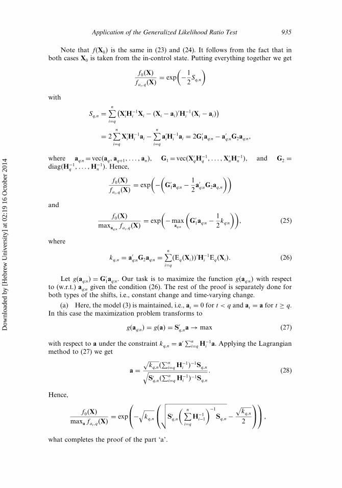
Application of the Generalized Likelihood Ratio Test 935

Note that f�X0� is the same in (23) and (24). It follows from the fact that inboth cases X0 is taken from the in-control state. Putting everything together we get

f0�X�fat�q�X�

= exp(−12Sq�n

)with

Sq�n =n∑

i=q

(X′

iH−1i Xi − �Xi − ai�

′H−1i �Xi − ai�

)= 2

n∑i=q

X′iH

−1i ai −

n∑i=q

a′iH−1i ai = 2G′

1aq�n − a′q�nG2aq�n�

where aq�n = vec�aq� aq+1� � � � � an�, G1 = vec�X′qH

−1q � � � � �X′

nH−1n �, and G2 =

diag�H−1q � � � � �H−1

n �. Hence,

f0�X�fat�q�X�

= exp(−(G′

1aq�n −12a′q�nG2aq�n

))and

f0�X�maxaq�n fat�q�X�

= exp(−max

aq�n

(G′

1aq�n −12kq�n

))� (25)

where

kq�n = a′q�nG2aq�n =n∑

i=q

�Eq�Xi��′H−1

i Eq�Xi�� (26)

Let g�aq�n� = G′1aq�n. Our task is to maximize the function g�aq�n� with respect

to (w.r.t.) aq�n given the condition (26). The rest of the proof is separately done forboth types of the shifts, i.e., constant change and time-varying change.

(a) Here, the model (3) is maintained, i.e., at = 0 for t < q and at = a for t ≥ q.In this case the maximization problem transforms to

g�aq�n� = g�a� = S′q�na → max (27)

with respect to a under the constraint kq�n = a′∑n

i=q H−1i a. Applying the Lagrangian

method to (27) we get

a =√kq�n�

∑ni=q H

−1i �−1Sq�n√

S′q�n�∑n

i=q H−1i �−1Sq�n

� (28)

Hence,

f0�X�maxa fat�q�X�

= exp

−√kq�n

√√√√S′

q�n

( n∑i=q

H−1i−1

)−1

Sq�n −√kq�n

2

�

what completes the proof of the part ‘a’.

Dow

nloa

ded

by [

Heb

rew

Uni

vers

ity]

at 0

2:19

16

Oct

ober

201

4

936 Bodnar

(b) Here, it is allowed the drift vector at to vary with the time. The controlchart is derived by maximizing g�aq�n� given (26). From the Lagrangian method weobtain

aq�n =√kq�n√

G′1G

−12 G1

G−12 G1� (29)

where

G′1G

−12 G1 =

n∑i=q

X′iH

−1i �H−1

i �−1H−1i Xi

=n∑

i=q

X′iH

−1i Xi = Dn −Dq−1�

Hence,

f0�X�maxa fat�q�X�

= exp

(−√kq�n

(√Dn −Dq−1 −

√kq�n

2

))� (30)

The theorem is proved.

Proof of Remark 3.1. Let f0�X� denote the joint density function of X0�X1� � � � �Xn

when the unknown parameters are replaced with the corresponding estimatedcounterparts. It holds that

f0�X� = f0�X � ��f����

where � is the vector with the estimated parameters. The last equality holds becausethe unknown parameters are estimated using previous data and, thus, they aremeasurable for all the sigma fields �i, i = 0� � � � � n− 1. Analogically, it holds that

fat�q�X� = fat�q�X � ��f���

for each q and at. Hence,

−2 ln Ln = −2 ln(

f0�X�

max1≤q≤n fat�q�X�

)= −2 ln

(f0�X�

max1≤q≤n fat�q�X�

)= −2 lnLn�

References

Alexander, C. (2000). Market Models. New York: Wiley.Bauwens, L., Laurent, S., Rombouts, J. V. K. (2006). Multivariate GARCH models:

a survey. J. Appl. Econometrics 21:79–109.Bodnar, O., Schmid, W. (2006). CUSUM control schemes for multivariate time series.

In: Lenz, H.-J., Wilrich, P.-Th., eds. Frontiers of Statistical Process Control, Vol. 8.Heidelberg: Physica, pp. 55–73.

Bodnar, O., Schmid, W. (2007). Surveillance of the mean behavior of multivariate time series.Statistica Neerlandica 61:1–24.

Dow

nloa

ded

by [

Heb

rew

Uni

vers

ity]

at 0

2:19

16

Oct

ober

201

4

Application of the Generalized Likelihood Ratio Test 937

Bollerslev, T. (1986). Generalized autoregressive conditional heteroscedasticity.J. Econometrics 31:307–327.

Bollerslev, T. (1990). Modeling the coherence in short-run nominal exchange rates:a multivariate generalized ARCH model. Rev. Econ. Statist. 72:498–505.

Bollerslev, T., Engle, R. F., Wooldridge, J. (1988). A capital asset pricing model with timevarying covariances. J. Polit. Econ. 96:116–131.

Broemeling, L. D., Tsurumi, H. (1987). Econometrics and Structural Change. New York:Marcel Dekker.

Comte, F., Lieberman, O. (2003). Asymptotic theory for multivariate GARCH processes.J. Multivariate Anal. 84:61–84.

Conte, S. D., de Boor, C. (1981). Elementary Numerical Analysis. London: McGraw-Hill.Crosier, R. B. (1988). Multivariate generalizations of cumulative sum quality control

schemes. Technometrics 30:291–303.Diebold, F. X., Nerlove, M. (1989). The dynamics of exchange rate volatility: a multivariate

latent factor ARCH model. J. Appl. Econometrics 4:1–21.Engle, R. F. (1982). Autoregressive conditional heteroscedasticity with estimates of the

variance of UK inflation. Econometrica 50:987–1008.Engle, R. F. (2002). Dynamic conditional correlation – a simple class of multivariate

GARCH models. J. Bus. Econ. Statist. 20(3):339–350.Engle, R. F. Ng, V. K. (1993). Measuring and testing the impact of news on volatility.

J. Fin. 48:1749–1778.Engle, R. F., Kroner, F. (1995). Multivariate simultaneous generalized ARCH. Econometric

Theor. 11:122–150.Engle, R. F. Sheppard, K. (2001). Theoretical and empirical properties of dynamic

conditional correlation multivariate GARCH. Unpublished paper: UCSD.Engle, R. F., Ng, V. K., Rothschild, M. (1990). Asset pricing with a factor-ARCH covariance

structure: empirical estimates for treasury bills. J. Econometrics 45:213–238.Gourieroux, C. (1997). ARCH Models and Financial Applications. New York: Springer.Greene, W. H. (2003). Econometric Analysis. Upper Saddle River, NJ: Prentice Hall.Harville, D. A. (1997). Matrix Algebra from a Statistician’s Perspective. New York:

Springer-Verlag.Hotelling, H. (1947). Multivariate quality control-illustrated by the air testing of sample

bombsights. In: Eisenhart, C., Hastay, M. W., Wallis, W. A., eds. Techniques of StatisticalAnalysis. New York: McGraw-Hill, pp. 111–184.

Jeantheau, T. (1998). Strong consistency of estimators for multivariate ARCH models.Econometric Theor. 14:70–86.

Knoth, S. Schmid, W. (2004). Control charts for time series: a review. In: Lenz, H.-J.,Wilrich, P.-Th., eds. Frontiers of Statistical Process Control, Vol. 7. Heidelberg: Physica,pp. 210–236.

Kramer, H., Schmid, W. (1997). EWMA charts for multivariate time series. Sequent. Anal.16(2):131–154.

Ling, S., McAleer, M. (2003). Asymptotic theory for a vector ARMA-GARCH model.Econometric Theor. 19:280–310.

Lowry, C. A., Woodall, W. H., Champ, C. W., Rigdon, S. E. (1992). A multivariateexponentially weighted moving average control chart. Technometrics 34:46–53.

Maddala, G. S., Kim, I.-M. (2002). Unit Roots, Cointegration, and Structural Change.Cambridge: Cambridge University Press.

Nelson, D. (1991) Conditional heteroscedasticity in stock returns: a new approach.Econometrica 59:347–370.

Ngai, H.-M., Zhang, J. (2001). Multivariate cumulative sum control charts based onprojection pursuit. Statistica Sinica 11:747–766.

Nikiforov, I. V. (1986). Sequential detection of changes in time series properties based on amodified cumulative sum algorithm. In: Telkamp, L., ed. Detection of Changes in RandomProcesses. New York: Optimization Software, pp. 142–150.

Dow

nloa

ded

by [

Heb

rew

Uni

vers

ity]

at 0

2:19

16

Oct

ober

201

4

938 Bodnar

Pignatiello, Jr., J. J., Runger, G. C. (1990). Comparison of multivariate CUSUM charts.J. Qual. Technol. 22:173–186.

Pollak, M., Siegmund, D. (1975). Approximations to the expected sample size of certainsequential tests. Annals of Statistics 3:1267–1282.

Siegmund, D. (1985). Sequential Analysis. New York, Berlin, Heidelberg, Tokyo: Springer.Tse, Y. K., Tsui, A. K. C. (2002). A multivariate generalized autoregressive conditional

heteroscedasticity model with time-varying correlations, J. Bus. Econ. Statist. 20(3):351–362.

van der Weide, R. (2002). GO-GARCH: a multivariate generalized orthogonal GARCHmodel. J. Appl. Econometrics 11:549–564.

Zakoian, J.-M. (1994). Threshold heteroscedastic models. J. Econ. Dynam. Control 14:45–52.

Dow

nloa

ded

by [

Heb

rew

Uni

vers

ity]

at 0

2:19

16

Oct

ober

201

4