Applications of Modern Data Collection and Modelling

Techniques to Biogeochemistry

GGR 403SEugene KwanMarch 2004

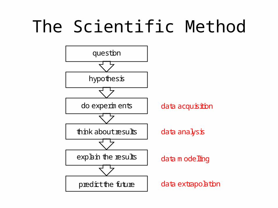
The Scientific Methodquestion

hypothesis

do experiments

think about results

explain the results

predict the future

data acquisition

data analysis

data modelling

data extrapolation

Data Acquisition

• Remote Sensing

• Isotopic Proxy Data/Mass Spectrometry

• Eddy Correlation Techniques

Remote Sensing

• Satellites, Airplanes, Ground-Based

• Uses spectrometers: instruments which analyze different parts of the electromagnetic spectrum

• “Passive vs. Active” Sensing– passive: satellite just gathers light– active: satellites emit energy

Satellite Orbits

• Geostationary: satellite stays over the same part of the Earth at all times

• Near-Polar: N/S orbits which, with the Earth’s E/W rotation, allow broad coverage

• Sun-Synchronous: Each area of the world is covered at the same local sun time

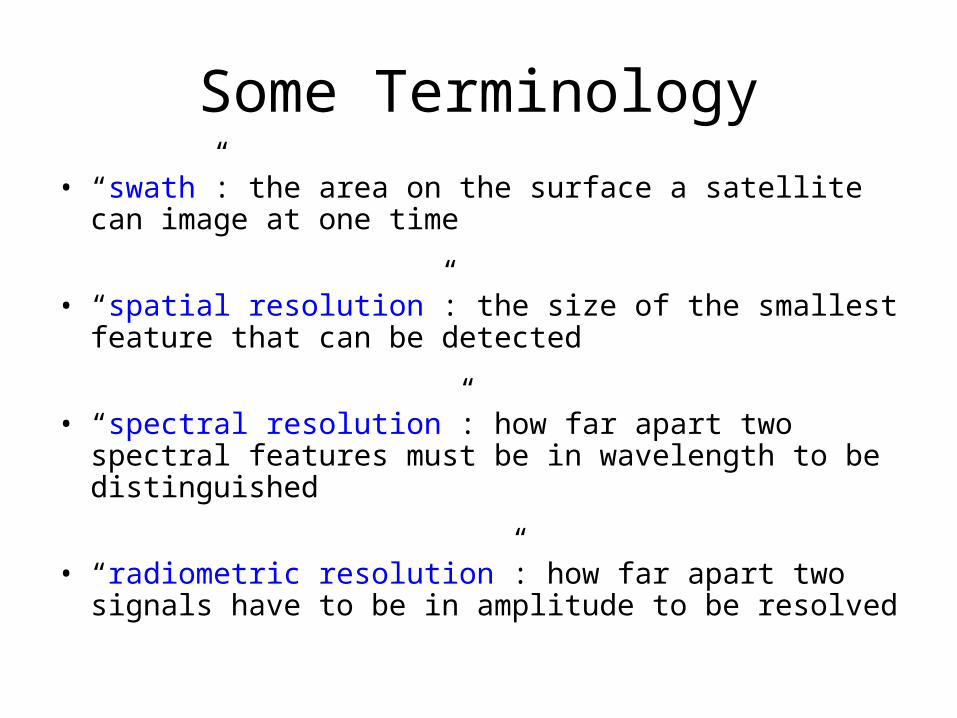
Some Terminology

• “swath”: the area on the surface a satellite can image at one time

• “spatial resolution”: the size of the smallest feature that can be detected

• “spectral resolution”: how far apart two spectral features must be in wavelength to be distinguished

• “radiometric resolution”: how far apart two signals have to be in amplitude to be resolved

Types of Sensing

• Optical/Stereoimages

• Multi-Spectral

• Thermal

• Weather

• Land-Observation

Stable Isotope RatioMass Spectrometry

• “proxy data”: a series of measurements which from which various historical parameters may be inferred

e.g. temperature may be inferred from

oxygen isotope ratios in carbonates

• typically used to reconstruct past climates

A Quick Review

• Atoms contain protons (positive charge), neutrons (no charge), and electrons (negative charge)

• The chemical properties of an atom depend principally on its atomic number: the number of protons

• Atoms are neutral:# protons = # electrons

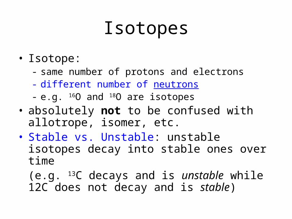
Isotopes

• Isotope: - same number of protons and electrons- different number of neutrons- e.g. 16O and 18O are isotopes

• absolutely not to be confused with allotrope, isomer, etc.

• Stable vs. Unstable: unstable isotopes decay into stable ones over time(e.g. 13C decays and is unstable while 12C does not decay and is stable)

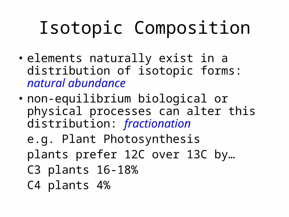
Isotopic Composition

• elements naturally exist in a distribution of isotopic forms: natural abundance

• non-equilibrium biological or physical processes can alter this distribution: fractionatione.g. Plant Photosynthesis

plants prefer 12C over 13C by…C3 plants 16-18%C4 plants 4%

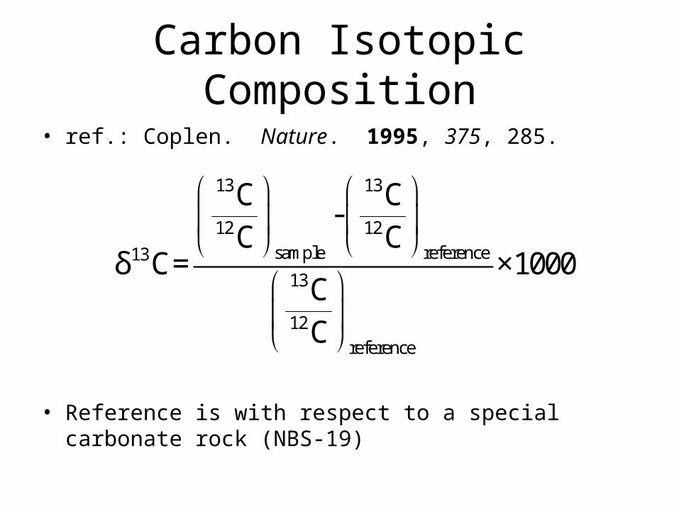
Carbon Isotopic Composition

• ref.: Coplen. Nature. 1995, 375, 285.

• Reference is with respect to a special carbonate rock (NBS-19)

13 13

12 12

sample reference13

13

12

reference

C C-

C Cδ C= ×1000

CC

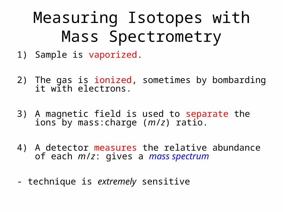
Measuring Isotopes withMass Spectrometry

1) Sample is vaporized.

2) The gas is ionized, sometimes by bombarding it with electrons.

3) A magnetic field is used to separate the ions by mass:charge (m/z) ratio.

4) A detector measures the relative abundance of each m/z: gives a mass spectrum

- technique is extremely sensitive

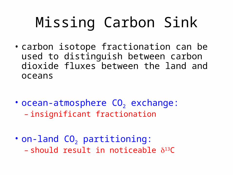
Missing Carbon Sink

• carbon isotope fractionation can be used to distinguish between carbon dioxide fluxes between the land and oceans

• ocean-atmosphere CO2 exchange:– insignificant fractionation

• on-land CO2 partitioning:– should result in noticeable 13C

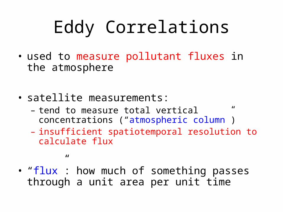
Eddy Correlations

• used to measure pollutant fluxes in the atmosphere

• satellite measurements:– tend to measure total vertical concentrations

(“atmospheric column”)– insufficient spatiotemporal resolution to calculate flux

• “flux”: how much of something passes through a unit area per unit time

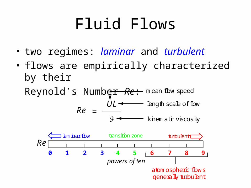
Fluid Flows

• two regimes: laminar and turbulent• flows are empirically characterized by their

Reynold’s Number Re:

ReUL

=

mean flow speed

length scale of flow

kinematic viscosity

powers of ten0 1 2 3 4 5 6 7 8

Relaminar flow turbulent

9

transition zone

atomospheric flowsgenerally turbulent

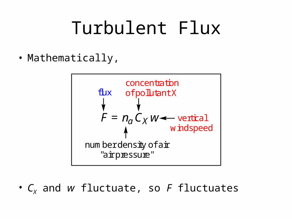
Turbulent Flux

• Mathematically,

• CX and w fluctuate, so F fluctuates

F = na CX w

flux

number density of air"air pressure"

concentrationof pollutant X

verticalwindspeed

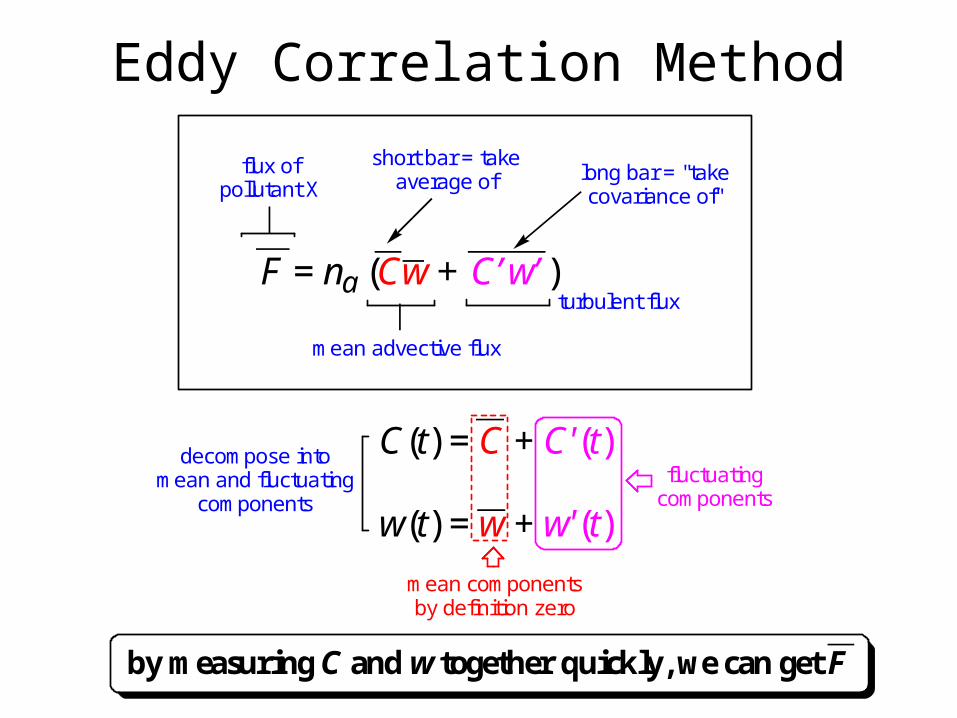
Eddy Correlation Method

F = na (Cw + C’w’)

flux ofpollutant X

mean advective flux

turbulent flux

long bar = "takecovariance of"

short bar = takeaverage of

C(t) = C + C'(t)

w(t) = w + w'(t)

decompose intomean and fluctuating

components

mean componentsby definition zero

fluctuatingcomponents

by measuring C and w together quickly, we can get F

Data Analysis

• “time series”: a set of measurements collected over time

Techniques:- Smoothing - Detrending

- Correlation/Autocorrelation/Convolution

- Fourier Transform (FT)

Data Smoothing

• data typically too noisy to work with

• would like to smooth it so trends can be observed

Two Methods:

1) Running Average/Running Mean

2) Running Median

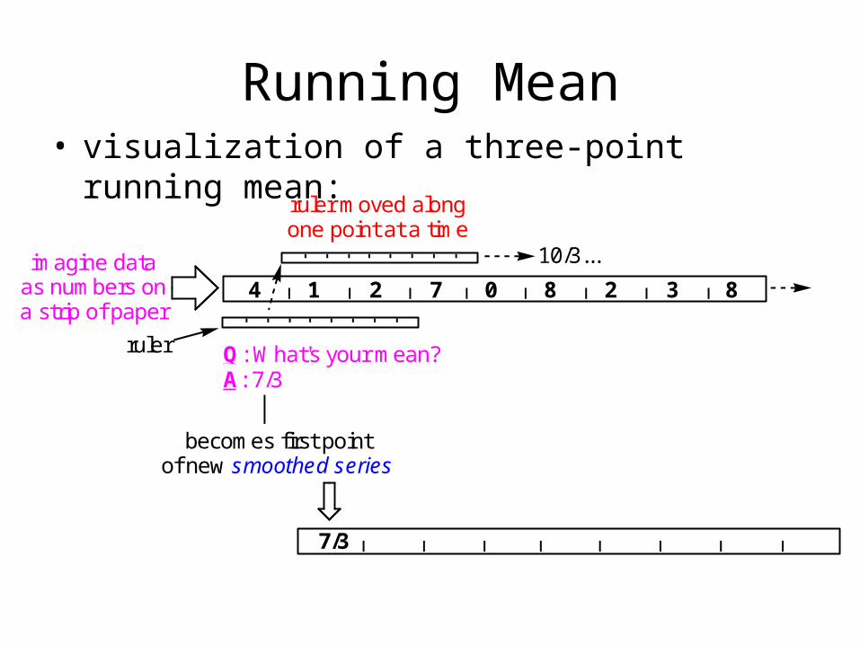
Running Mean• visualization of a three-point running mean:

4 1 2 7 0 8 2 3 8imagine data

as numbers ona strip of paper

Q: What's your mean?A: 7/3

becomes first pointof new smoothed series

7/3

ruler

ruler moved alongone point at a time

10/3...

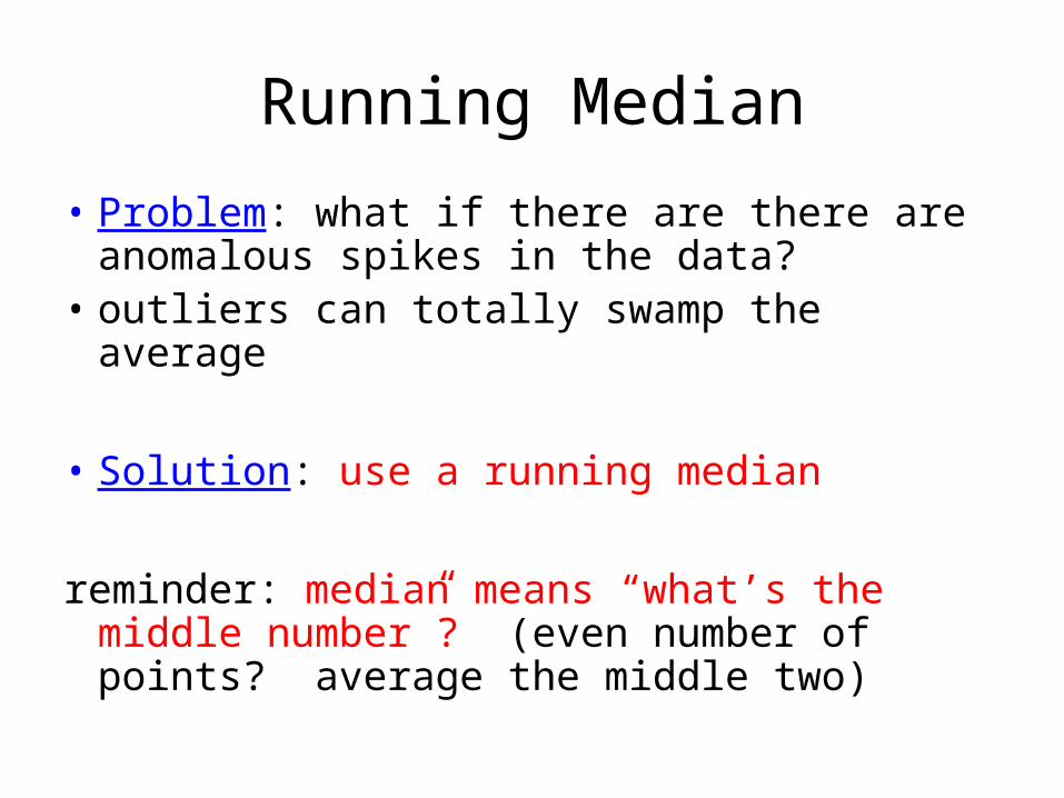
Running Median

• Problem: what if there are there are anomalous spikes in the data?

• outliers can totally swamp the average

• Solution: use a running median

reminder: median means “what’s the middle number”? (even number of points? average the middle two)

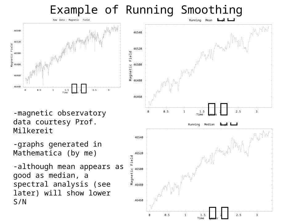
Example of Running Smoothing

0 0.5 1 1.5 2 2.5 3Timeyears46440

46460

46480

46500

46520

46540

citengaMdleiF

Raw Data : Magnetic Field

0 0.5 1 1.5 2 2.5 3Timeyears

46460

46480

46500

46520

46540

citengaMdleiF

Running Mean3 pt

0 0.5 1 1.5 2 2.5 3Timeyears

46460

46480

46500

46520

46540

citengaMdleiF

Running Median3 pt-magnetic observatory data courtesy Prof. Milkereit

-graphs generated in Mathematica (by me)

-although mean appears as good as median, a spectral analysis (see later) will show lower S/N

Correlation Methods

• purposes:1) find periodicities in data2) relate two data sets3) subtract instrumental effects

Methods:- auto- and cross- correlation- convolution

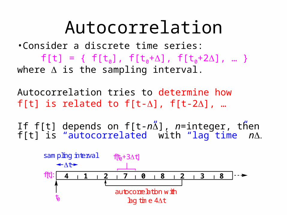
Autocorrelation•Consider a discrete time series:

f[t] = { f[t0], f[t0+], f[t0+2], … }where is the sampling interval.

Autocorrelation tries to determine howf[t] is related to f[t-], f[t-2], …

If f[t] depends on f[t-n], n=integer, then f[t] is “autocorrelated” with “lag time” n

4 1 2 7 0 8 2 3 8

t0

tsampling interval

autocorrelation withlag time 4t

f[t0+3t]

f[t]:

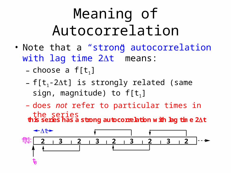
Meaning of Autocorrelation

• Note that a “strong autocorrelation with lag time 2t” means:– choose a f[t1]

– f[t1-2t] is strongly related (same sign, magnitude) to f[t1]

– does not refer to particular times in the series

2 3 2 3 2 3 2 3 2

t0

t

this series has a strong autocorrelation with lag time 2t

f[t]:

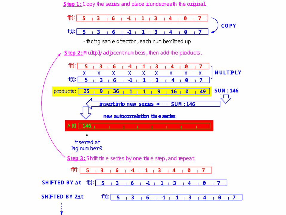
5 3 6 -1 1 3 4 0 7

Step 1: Copy the series and place it underneath the original.

f[t]:

5 3 6 -1 1 3 4 0 7f[t]:COPY

- facing same direction, each number lined up

Step 2: Multiply adjacent numbers, then add the products.

5 3 6 -1 1 3 4 0 7f[t]:

5 3 6 -1 1 3 4 0 7f[t]:MULTIPLYX XXXXXXXX

25 9 36 1 1 9 16 0 49products: SUM: 146

SUM: 146

146A[t]

new autocorrelation time series

insert into new series

inserted atlag number 0

Step 3: Shift time series by one time step, and repeat.

5 3 6 -1 1 3 4 0 7f[t]:

5 3 6 -1 1 3 4 0 7f[t]:SHIFTED BY t

5 3 6 -1 1 3 4 0 7f[t]:SHIFTED BY 2t

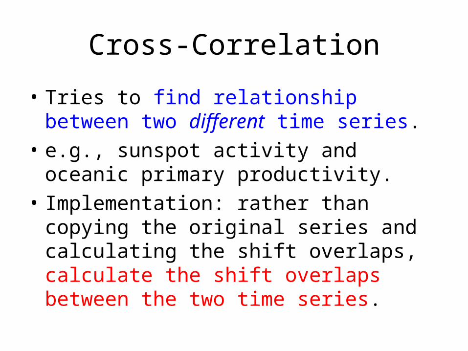
Cross-Correlation

• Tries to find relationship between two different time series.

• e.g., sunspot activity and oceanic primary productivity.

• Implementation: rather than copying the original series and calculating the shift overlaps, calculate the shift overlaps between the two time series.

Convolution/Deconvolution

• Mathematically more complex• Useful for

– Combining measurements taken from different instruments

– Distinguishing real signals from instrumental noise

• Its opposite, decovolution, can decompose two overlapping signals into their components.

Data Modelling

• One Box Model

• Lifetime

• First-Order Approximation

• Steady States/Dynamic Equilibria

• Multibox Models/General Circulation Models

Data Extrapolation

• Will consider the carbon cycle in terms of a simple multi-box model

• Will account for pH and solubility of carbon dioxide in the oceans

• Will make some lifetime estimates and other predictions