Embed Size (px)
Citation preview

Applications of Reformulations inMathematical Programming
These presentee pour obtenir le grade de
DOCTEUR DE L’ECOLE POLYTECHNIQUE
par
Alberto Costa
Soutenue le 18 septembre 2012 devant le jury compose de:
Eligius M. T. Hendrix Wageningen University, Wageningen Rapporteur
Arnaud Pecher Universite de Bordeaux I, Bordeaux Rapporteur
Olivier Bournez Ecole Polytechnique, Palaiseau Examinateur
A. Ridha Mahjoub Universite Paris Dauphine (Paris 9), Paris Examinateur
Roberto Wolfler Calvo Universite Paris Nord (Paris 13), Paris Examinateur
Pierre Hansen GERAD, HEC, Montreal Directeur de these
Leo Liberti Ecole Polytechnique, Palaiseau Directeur de these
Ider Tseveendorj UVSQ, Versailles Directeur de these


Premature optimization is the root of all evil.
Donald Ervin Knuth
i

ii

Abstract
Mathematical programming is a technique that can be used to solve real-world opti-
mization problems, where one wants to maximize, or minimize, an objective function
subject to some constraints on the decision variables. The key features of mathe-
matical programming are the creation of a model for describing the problem (the so
called formulation), and the implementation of efficient algorithms to solve it (also
called solvers). In this thesis, we focus on the first point. More precisely, we study
some problems arising from different domains, and starting from the most natu-
ral models for describing them, we propose alternative formulations, which share
some properties with the original models but are somehow better (for instance in
terms of computational time needed to obtain the solution by the solver). These
new models are called reformulations. We follow the classification of reformulations
proposed by Liberti in [Reformulations in Mathematical Programming: Definitions
and Systematics, RAIRO-OR, 43(1):55-86, 2009]: exact reformulations (also called
opt-reformulations), narrowings, relaxations. This thesis is concerned with three
mathematical programming applications where the reformulation was crucial to ob-
tain a good solution. The first problem tackled herein is graph clustering by means
of modularity maximization. Since this problem is NP-hard, several heuristics are
proposed. We focus on a divisive hierarchical algorithm which works by recursively
splitting a cluster into two new clusters in an optimal way. This splitting step is per-
formed by solving a convex binary quadratic program. This is reformulated exactly
to a more compact form without changing the optimal solutions set (exact reformu-
lation). We also evaluate the impact provided by the reduction of the number of
symmetric global optima of the problem, which is also an important topic of the next
part of this thesis. The computational times are considerably reduced with respect
to the original formulation. The second problem tackled in the thesis is the Packing
of Equal Circles in a Square (PECS), where one wants to place non-overlapping
equal circles in a unit square in such a way as to maximize the common radius. One
of the reasons why the problem is hard to solve is the presence of several symmetric
optimal solutions, and consequently a very large Branch-and-Bound tree. Some of
the symmetric optima are made infeasible by adjoining some Symmetry Breaking
iii

Constraints (SBCs) to the formulation, thereby obtaining a narrowing. Both compu-
tational time and size of the Branch-and-Bound tree outperform the ones provided
by the original formulation. The third application considered in the thesis is that of
computing the convex relaxation for multilinear problems, and to compare the “pri-
mal” formulation and another one obtained using a “dual” representation. Although
these two relaxations are both already known in the literature, we make a striking
observation, i.e., that the dual relaxation leads to a faster and more stable solution
process as regards CPU time.
iv

Resume
La programmation mathematique est une technique qui peut etre utilisee pour re-
soudre des problemes concrets ou l’on veut maximiser, ou minimiser, une fonction
objectif soumise a des contraintes sur les variables decisionnelles. Les caracteristiques
les plus importantes de la programmation mathematique sont la creation d’un mo-
dele pour decrire le probleme (aussi appele formulation), et la mise en œuvre d’al-
gorithmes efficaces pour le resoudre (aussi appeles solveurs). Dans cette these, on
s’occupe du premier point. Plus precisemment, on etudie certains problemes qui pro-
viennent de domaines differents, et en commencant par les modeles les plus naturels
pour les decrire, on presente des formulations alternatives, qui partagent certaines
proprietes avec le modele original mais qui sont en quelque sorte meilleures (par
exemple au niveau du temps d’execution necessaire pour obtenir la solution par le
solveur). Ces nouveaux modeles sont appeles reformulations. On suit la classifica-
tion des reformulations proposee par Liberti dans [Reformulations in Mathematical
Programming: Definitions and Systematics, RAIRO-OR, 43(1):55-86, 2009] : exact
reformulations (aussi appellees opt-reformulations), narrowings, relaxations. Cette
these concerne trois applications de la programmation mathematique ou les reformu-
lations ont ete fondamentales pour obtenir une bonne solution. Le premier probleme
etudie est le partitionnement de graphes sur la base de la maximisation de la modu-
larite. Comme ce probleme est NP-difficile, plusieurs heuristiques sont proposees.
On s’occupe d’un algorithme separatif hierarchique qui fonctionne en divisant re-
cursivement une classe en deux nouvelles classes de facon optimale. Cet etape de
division est accomplie en resolvant un programme binaire quadratique et convexe. Il
est reformule de maniere exacte pour obtenir une forme plus compacte sans modifier
l’ensemble des solutions optimales (exact reformulation). On considere aussi l’impact
donne par la reduction du nombre des solutions symetriques globalement optimales.
Les temps d’execution sont considerablement reduits par rapport a la formulation
originelle. Le deuxieme probleme etudie dans cette these est le placement de cercles
egaux dans un carre (Packing Equal Circles in a Square, ou PECS), ou l’on veut
placer des cercles egaux dans un carre de cote 1 sans avoir de superposition et en
maximisant le rayon commun. L’une des raisons pour laquelle le probleme est dif-
v

ficile a resoudre vient de la presence de plusieurs solutions symetriques optimales,
et par consequent un arbre de separation-et-evaluation (ou Branch-and-Bound) tres
large. Certaines solutions symetriques optimales sont rendues irrealisables en ajou-
tant des contraintes pour briser les symetries (Symmetry Breaking Constraints, ou
SBCs) a la formulation, en obtenant ainsi un narrowing. Le temps d’execution et la
dimension de l’arbre de Branch-and-Bound sont tous les deux meilleurs par rapport
a la formulation originelle. La troisieme application consideree dans cette these est
le calcul de la relaxation convexe pour des problemes multilineaires, et la comparai-
son de la formulation “primale” avec celle obtenue par une representation “duale”.
Bien que ces deux relaxations soient deja connues, il est interessant de voir que la
relaxation duale conduit a des meilleures performances de calcul.
vi

Acknowledgements
I wish to thank several people. First of all, my supervisors: Pierre Hansen, Leo
Liberti, and Ider Tseveendorj. They gave me the possibility to work on interesting
topics, and to present my results in many interesting (and beautiful) places around
the world. One of these is Paris, where I spent most of these three years. This
experience was very important, both for my professional and personal life. All this
was made possible by means of Digiteo’s financial support under contract 2009-55D
“ARM”.
I would also like to thank my friends. Alena, because she allows me to see the
world from another point of view. Fabio and Francesca, for their friendship and
help, as well as for the poker tournaments. Alessandra, Alvaro, Anna, Arabella,
Cesar, Claire, Claudia, David, Dimo, Dominik, Emanuele, Eugenio, Hassan, Irene,
Jennifer, Jerome, Katya, Lorenzo, Lucio, Mahsa, Marc, Marco, Maria, Nives, Ryna,
Sonia, Xue, and my friends in Italy.
Moreover, I thank my Master thesis’ supervisor, prof. Massimo Melucci, for his
suggestions and many interesting discussions.
Finally, I would like to thank my family for their support and love.
vii

viii

Acronyms
• ASC: Almost-Strong Communities detection algorithm for clustering problem;
• BB: Branch-and-Bound;
• BMM: Bipartite Modularity Maximization;
• cMINLP: convex Mixed Integer Nonlinear Programming;
• cMIQP: convex Mixed Integer Quadratic Programming;
• cNLP: convex Nonlinear Programming;
• CPP: Circle Packing Problem;
• DAG: Directed Acyclic Graph;
• e.g.,: exempli gratia, in Latin. It means “for example”;
• i.e.,: id est, in Latin. It means “that is”;
• KKT: Karush-Kuhn-Tucker conditions;
• LP: Linear Programming;
• MILP: Mixed Integer Linear Programming (synonym of MIP);
• MINLP: Mixed Integer Nonlinear Programming;
• MIP: Mixed Integer Programming (synonym of MILP);
• MM: Modularity Maximization;
• MP: Mathematical Programming;
• NLP: Nonlinear Programming;
• PECS: Packing Equal Circles in a Square;
• PPS: Point Packing in a Square;
• QCQP: Quadratically Constrained Quadratic Problem;
• sBB: spatial Branch-and-Bound;
• SBC: Symmetry Breaking Constraint;
• SC: Strong Communities detection algorithm for clustering problem;
• SQP: Sequential Quadratic Programming;
• s.t.: subject to;
• WLOG: Without Loss Of Generality.
ix

x

Contents
1 Introduction 1
1.1 Motivations . . . . . . . . . . . . . . . . . . . . . . . . . . . . . . . . 1
1.2 Mathematical programming . . . . . . . . . . . . . . . . . . . . . . . 3
1.2.1 Classification of mathematical programming problems . . . . 4
1.2.1.1 Convexity . . . . . . . . . . . . . . . . . . . . . . . . 4
1.2.1.2 Classes of mathematical programming problems . . 6
1.2.2 Approaches to solve mathematical programming problems . . 7
1.2.2.1 Linear programming . . . . . . . . . . . . . . . . . . 8
1.2.2.2 Mixed integer linear programming . . . . . . . . . . 8
1.2.2.3 Nonlinear and convex nonlinear programming . . . 11
1.2.2.4 Convex mixed integer nonlinear programming . . . 13
1.2.2.5 Mixed integer nonlinear programming . . . . . . . . 14
1.3 Reformulations . . . . . . . . . . . . . . . . . . . . . . . . . . . . . . 15
1.3.1 Classification of reformulations . . . . . . . . . . . . . . . . . 16
1.3.1.1 Exact reformulations . . . . . . . . . . . . . . . . . 17
1.3.1.2 Narrowings . . . . . . . . . . . . . . . . . . . . . . . 17
1.3.1.3 Relaxations . . . . . . . . . . . . . . . . . . . . . . . 18
1.4 Contributions . . . . . . . . . . . . . . . . . . . . . . . . . . . . . . . 18
I An application of exact reformulations 21
2 Clustering in general and bipartite graphs 25
2.1 Definitions and notation . . . . . . . . . . . . . . . . . . . . . . . . . 27
2.2 Clustering based on modularity maximization . . . . . . . . . . . . . 28
2.2.1 Hierarchical divisive heuristic . . . . . . . . . . . . . . . . . . 30
2.2.1.1 Reduction of number of variables and constraints . 33
2.2.1.2 Binary decompositions . . . . . . . . . . . . . . . . 36
2.2.1.3 Symmetry breaking constraint . . . . . . . . . . . . 39
2.2.1.4 Numerical results . . . . . . . . . . . . . . . . . . . 39
xi

2.2.2 Extension to bipartite graphs . . . . . . . . . . . . . . . . . . 42
2.2.2.1 Fortet linearization . . . . . . . . . . . . . . . . . . 44
2.2.2.2 Square reformulation . . . . . . . . . . . . . . . . . 46
2.2.2.3 Binary decomposition . . . . . . . . . . . . . . . . . 48
2.2.2.4 Numerical results . . . . . . . . . . . . . . . . . . . 49
2.3 Clustering based on strong and almost-strong conditions . . . . . . . 52
2.3.1 Strong communities detection . . . . . . . . . . . . . . . . . . 55
2.3.2 Almost-strong communities detection . . . . . . . . . . . . . 58
2.3.3 Comparison between SC and ASC . . . . . . . . . . . . . . . 60
2.4 Conclusions . . . . . . . . . . . . . . . . . . . . . . . . . . . . . . . . 64
II An application of narrowings 67
3 Circle packing in a square 71
3.1 Mathematical programming formulations . . . . . . . . . . . . . . . 75
3.2 Detection of symmetries for circle packing . . . . . . . . . . . . . . . 76
3.2.1 Definitions and notation . . . . . . . . . . . . . . . . . . . . . 80
3.2.2 Automatic symmetry detection . . . . . . . . . . . . . . . . . 80
3.2.3 Symmetric structure of circle packing . . . . . . . . . . . . . 82
3.3 Order symmetry breaking constraints . . . . . . . . . . . . . . . . . 84
3.3.1 Weak constraints . . . . . . . . . . . . . . . . . . . . . . . . . 84
3.3.2 Strong constraints . . . . . . . . . . . . . . . . . . . . . . . . 84
3.3.3 Mixed constraints . . . . . . . . . . . . . . . . . . . . . . . . 86
3.3.4 Numerical results . . . . . . . . . . . . . . . . . . . . . . . . . 88
3.4 Other constraints . . . . . . . . . . . . . . . . . . . . . . . . . . . . . 90
3.4.1 Fixing points symmetry breaking constraints . . . . . . . . . 90
3.4.2 Bounds symmetry breaking constraints . . . . . . . . . . . . 93
3.4.3 Triangular inequality constraints . . . . . . . . . . . . . . . . 94
3.4.4 Numerical results . . . . . . . . . . . . . . . . . . . . . . . . . 95
3.5 A conjecture about the reduction of the search space . . . . . . . . . 96
3.6 Conclusions . . . . . . . . . . . . . . . . . . . . . . . . . . . . . . . . 99
III An application of relaxations 101
4 Primal and dual convex relaxations for multilinear terms 105
4.1 Definitions and notation . . . . . . . . . . . . . . . . . . . . . . . . . 106
4.2 Primal relaxation . . . . . . . . . . . . . . . . . . . . . . . . . . . . . 107
4.2.1 Bilinear terms . . . . . . . . . . . . . . . . . . . . . . . . . . 108
4.2.1.1 McCormick’s inqualities . . . . . . . . . . . . . . . . 109
4.2.1.2 Fortet inequalities . . . . . . . . . . . . . . . . . . . 109
xii

4.2.2 Trilinear terms: Meyer-Floudas inequalities . . . . . . . . . . 110
4.2.3 Quadrilinear terms . . . . . . . . . . . . . . . . . . . . . . . . 111
4.3 Dual relaxation . . . . . . . . . . . . . . . . . . . . . . . . . . . . . . 111
4.3.1 Example . . . . . . . . . . . . . . . . . . . . . . . . . . . . . . 112
4.4 Comparison and numerical results . . . . . . . . . . . . . . . . . . . 113
4.5 Conclusions . . . . . . . . . . . . . . . . . . . . . . . . . . . . . . . . 114
IV Conclusions and bibliography 117
5 Conclusions 119
Bibliography 123
xiii

xiv
Chapter 1Introduction
1.1 Motivations
The aim of Mathematical Programming (MP) is to analyze and solve optimization
problems. These involve the minimization (or maximization) of one (or possibly
more) objective functions subject to some constraints expressed in terms of the
decision variables. Several problems, arising from various domains (e.g., artificial
intelligence [50, 137], bioinformatics and computational biology [92, 113, 147, 150,
161, 162, 192–194, 249], chemistry and chemical engineering [14, 111, 163, 167, 177],
graph clustering [79, 121], engineering [16, 125, 226], location [41, 120, 146], medicine
[86,166,168,176,181,227], physics [149], transportation [12,21,229]), can be described
in this way. Nevertheless, it is not always possible to easily solve such problems
because of the size of the instances, nonlinearity and/or nonconvexity of the objective
function and/or constraints, uncertainty in the input data, and other causes.
In the last decades the research carried out to solve more and more complex
problems has followed two main directions: first, an improvement of the solvers and
algorithms, taking also into account the increasing power of computers. Second, the
way to model problems. These two aspects are in fact two sides of the same coin,
since a good solution of an optimization problem is obtained by means of both an
appropriate model (also called formulation) and an efficient algorithm to solve it.
More precisely, the process which leads from a real-world problem to its solution by
means of MP can be resumed in the following 4 steps, summarized in Figure 1.1:
1. formalize the (real-world) problem;
2. create an abstract mathematical model to describe the problem;
3. give the model as input to a solver in order to obtain the optimal solution (if
the solution process is too much time and/or memory demanding due to the
difficulty of the problem, and the optimal solution cannot be found, usually

2 Chapter 1. Introduction
the solver can provide some other informations as the best solution found so
far and sometimes a bound on the cost of the optimal solution);
4. interpret the solution within the real-world setting of the problem.
Figure 1.1: Solution process for a problem using MP (the picture is taken fromhttp://www.eudoxus.com/).
Although the use of an efficient solver is very important, it is just as important
to model the problem appropriately, as it directly affects solver’s performance and
the possibility to map the optimal solution into the real-world domain. Regarding
the importance of solvers and computer power, and considering for instance linear
optimization, during the Panel session of the 1st International Conference on Op-
erations Research and Enterprise Systems (ICORES) held in Portugal on February
2012, Dominique De Werra (professor at Ecole Polytechnique Feredale de Lausanne
and president of IFORS1 from 2010 to 2012) recalled that from 1988 to 2003 the im-
provement of computers power can be estimated as 800x, whereas the improvement
of the efficiency of algorithms as 2.360x, giving a global acceleration of almost two
million fold. More details can be found in [30]. Note that in this thesis we mostly
consider general-purpose solvers, and we focus on the design of efficient MP models.
However, given a problem, one can design a specific algorithm to solve it, as done
for example in Section 2.3.
Concerning the models, the most natural way to describe a problem often leads
to a formulation which might not be the best for a given solver. Therefore, starting
from a first formulation, one tries to modify it in order to obtain an alternative
formulation, called reformulation, which is somehow better (for instance in term of
computational time needed by the solver to obtain the optimal solution). Unlike the
previous point about algorithms and computational power, it is not easy to estimate
how much one can gain by reformulating a problem in the general case, since this
depends on the problem itself and also on the features of the solver which can be
exploited by the new formulation. Furthermore, after reformulating a problem, one
1IFORS is the International Federation of Operational Research Society; it has been foundedin 1953 by UK, USA and France, and now counts more than 50 national societies. Its role is topromote the development of Operations Research worldwide.
1.2. Mathematical programming 3
could employ alternative (and more efficient) solvers. For instance, if a nonlinear
problem can be reformulated as a linear one, one may take advantage of powerful
solvers such as CPLEX [135] or Gurobi [117], which are usually more robust than
the nonlinear ones. For example, consider a problem which is nonlinear due to
the presence of products between binary variables. It can be reformulated exactly
(i.e., without changing the set of optimal solutions) as an integer linear problem
by means of the Fortet’s inequalities, which are introduced in Sections 2.2.1.1 and
4.2.1.2. However, given an optimization problem and a solution algorithm, there
exists a formulation of the problem that is optimal with respect to the CPU time
taken by the algorithm to solve it (again, in case of problems where the optimal
solution cannot be found in a reasonable amount of time, other parameters can
be considered, such as the best solution or the best bound found so far). The
reformulated model should be as close as possible to this best formulation.
Another important application of reformulations arises when considering MP
languages such as AMPL [97] or GAMS [42]. Each solution algorithm requires
the problem to be cast in a particular form, called standard form; for instance,
the simplex algorithm [70] requires linear equality constraints only with inequalities
limited to the variable bounds. The reformulation of the problem into the standard
form for the chosen solver is carried out automatically, thus the users are free to
focus on modeling rather than worrying about algorithmic details. Other examples
of automatic reformulations are presented in [7, 158].
It turns out that the field of reformulations is very important and can have a
high impact in both academia and industry. Thus, the motivations of this thesis are
mainly two: first, to perform an analysis of different problems, trying to understand
which is the best way to reformulate them, and moving toward the best formulation.
Second, to show the impact of different reformulation techniques when applied to
these problems.
The rest of this chapter is organized as follows: in Section 1.2 we present MP,
while in Section 1.3 we introduce the theory and classification of reformulations,
mainly based on the work presented in [157]. Finally, in Section 1.4 we summarize
the main contributions of this thesis.
1.2 Mathematical programming
There exist several definitions of MP. One can simply state that MP is a branch of
Operations Research which can be employed to analyze and solve real-world prob-
lems where one wants to maximize, or minimize, an objective function subject to
some constraints on the decision variables. A more “applications-oriented”definition
(related to the historical origin of MP as tool to solve problems arising in the army
field), taken from [38], is the following:

4 Chapter 1. Introduction
It concerns the optimum allocation of limited resources among competing
activities, under a set of constraints imposed by the nature of the prob-
lem being studied. These constraints could reflect financial, technological,
marketing, organizational, or many other considerations. In broad terms,
mathematical programming can be defined as a mathematical represen-
tation aimed at programming or planning the best possible allocation of
scarce resources.
Indeed, these definitions are not formal, but helpful to understand what is MP
and what kind of problems it can deal with. Moving toward a more precise definition,
we can express a generic MP formulation as:
min f(x)
s.t. x ∈ X,(1.1)
where X is the set of feasible solutions, and it is a cartesian product of continuous
and discrete intervals (as it is defined by the constraints of the problem and the
bounds on the variables), and f : X → RF represents the set of |F | objective
functions (if |F | > 1 we have a multiobjective problem; in this thesis we always
consider problems where |F | = 1). The problem represented by the model (1.1) can
be expressed as: find a point x∗ ∈ X (called optimal solution or global optimum)
which minimizes the objective function f(x), that is ∀x ∈ X f(x∗) ≤ f(x). In the
rest of the thesis we consider as global optimum the solution x∗, and f(x∗) its cost,
so in this sense all the different solutions having as cost f(x∗) are global optima. A
point x ∈ X is called local optimum if ∃ ǫ > 0 | ∀x ∈ X, ‖x− x‖ ≤ ǫ it holds that
f(x) ≤ f(x), i.e., there are not better solutions than f(x) in the neighborhood of
x. If a problem does not admit any optimal solution, it is called infeasible problem,
that is X = ∅. If there exist many optimal solutions, the standard general-purpose
solvers usually only find one solution, though the modern solvers have options for
finding more.
1.2.1 Classification of mathematical programming problems
In this section we propose a classification of MP problems. Before doing that, a
very important concept must be introduced: convexity. Note that in the rest of this
chapter we always refer to minimization problems. A maximization problem where
one wants to maximize an objective function f can be reformulated as a minimization
problem by means of the relationship max f = −min−f .
1.2.1.1 Convexity
For a class of problems, namely convex problems in form of minimization, the set
of global optima is the same as the set of local optima. Intuitively, they are easier
to solve, since there is no need to continue the search for a global optimum after

1.2. Mathematical programming 5
having found a local optimum, whilst in general this is not true. In order to define
more formally convexity, some definitions (mostly taken from [87]) are introduced
in the following:
Definition 1.2.1 (Convex combination [87]). The convex combination of k
points x1, . . . , xk ∈ Rn is defined as z =
∑ki=1 λixi, where ∀i ∈ 1, . . . , k λi ≥ 0
and∑k
i=1 λi = 1. If λ ∈ (0, 1)k, then z is called strict convex combination.
When k = 2, the previous definition can be reformulated as follows: given two
points x, y ∈ Rn, its convex combination z is defined as z = λx + (1 − λ)y where
λ ∈ [0, 1] (strict if λ ∈ (0, 1)). For the sake of clarity, in the following definitions we
consider the case when k = 2.
Definition 1.2.2 (Convex set [87]). A set X ⊆ Rn is called convex if ∀x, y ∈ X,
it holds that X contains all the convex combinations z of x and y, that is z =
λx+ (1− λ)y ∈ X, ∀λ ∈ [0, 1].
It also holds that intersection of convex sets is a convex set. An example of
convex and nonconvex sets is depicted in Figure 1.2.
(a) (b)
Figure 1.2: Examples of convex set (a) and nonconvex set (b).
Definition 1.2.3 (Convex function [87]). A function f : X → R defined on a
convex set X ⊆ Rn is called convex if ∀x, y ∈ X, ∀λ ∈ [0, 1], it holds that f(z) ≤
λf(x) + (1 − λ)f(y), where z = λx + (1 − λ)y. If λ ∈ (0, 1) and ∀x 6= y f(z) <
λf(x) + (1− λ)f(y) then f is called strict convex function.
A graphical representation of a convex function is given in Figure 1.3. It is inter-
esting to underline some facts: (i) if a function g(x) is convex, then the constraints
having the form g(x) ≤ b, b ∈ R are convex. In general, g(x) ≥ b could be a non-
convex constraint, even if g(x) is a convex function. In the case of g(x) convex,
the constraint g(x) ≥ b is called reverse convex [240]; (ii) if g(x) is linear, g(x)O b,
where O ∈ ≤,=,≥ is a convex constraint; (iii) if the set of feasible solutions X is
defined by convex constraints, then it is convex. We can now introduce the following
theorem:

6 Chapter 1. Introduction
Figure 1.3: Convex function f
Theorem 1.2.4 (Property of optimal solutions for convex problems [87]).
Consider a convex problem, that is a problem stated in the form (1.1) where X ⊆ Rn
is a convex set, and the objective function to be minimized f : X → R is a convex
function. Each local optimum is also a global optimum.
Another important concept, that is concavity, is strictly related to convexity.
More precisely, substituting ≤ and < with ≥ and > in Definition 1.2.3, we obtain
the definitions of concave and strict concave function. These concepts are useful in
the case of MP problem stated as maximization problems. The role of convexity
and concavity in MP can be summarized by these facts [38]:
• A local minimum (maximum) of a convex (concave) function on a convex
feasible region is also a global minimum (maximum).
• A local minimum (maximum) of a strict convex (concave) function on a convex
feasible region is the unique global minimum (maximum).
1.2.1.2 Classes of mathematical programming problems
We can now propose a classification of the MP problems formulated in the very
general form (1.1). Remember that the set X is given by the bounds and kinds
(as integer, continuous, or discrete) of the variables, and by the constraints of the
problem, which are usually on the form g(x) ≤ 0 or g(x) = 0.
• Linear Programming (LP): the objective function and the constraints are lin-
ear, and the variables are continuous;
• Mixed Integer Linear Programming (MILP or MIP): the objective function
and the constraints are linear, and at least one variable is integer;2
2Actually MILP is a special case of NLP, as the integrality of a variable xj can be expressedby the nonlinear constraint sin(πxj) = 0. Nevertheless MILP is separated from NLP because thereexist specific techniques to solve integer problems, as shown in Section 1.2.2.2. If all the variablesare integer, sometimes ILP (Integer Linear Programming) is used in place of MILP to refer to theproblem.

1.2. Mathematical programming 7
• convex Nonlinear Programming (cNLP): the objective function and the con-
straints are convex with at least one of them being nonlinear, and the variables
are continuous;
• Nonlinear Programming (NLP): at least one among the objective function and
the constraints is nonlinear, and the variables are continuous;
• convex Mixed Integer Nonlinear Programming (cMINLP): the objective func-
tion and the constraints are convex with at least one of them being nonlinear,
and at least one variable is integer;
• Mixed Integer Nonlinear Programming (MINLP): at least one among the ob-
jective function and the constraints is nonlinear, and at least one variable is
integer.
We can further write the following relationships: LP ⊂ MILP ⊂ cMINLP ⊂ MINLP
and LP ⊂ cNLP ⊂ NLP ⊂ MINLP. The meaning is that if a solver can be employed
for a given class of problems C, then it can also be employed for problems of all
the classes D ⊂ C. For instance, a MINLP solver can be employed to solve a NLP
problem, but a NLP solver working on a MINLP instance will ignore the integrality
constraints on the variables. These relationships give also an intuitive idea about
the complexity of the problems of the different categories. In general D ⊂ C means
that D is easier to solve than C. Hence, LP problems are usually the easiest to
solve, whereas MINLPs are the most difficult. Note that usually convex problems
are easier to solve than nonconvex ones, since, in the former, local optima are also
global optima, as explained earlier.
It is possible to go further into detail with the categorization of MP problems, but
for this thesis the previous classification suffices. The clustering problems presented
in Chapter 2 are MINLPs and cMINLPs, and we reformulate them as MILPs. In
Chapter 3 the Packing Equal Circles in a Square (PECS) problem is an example
of nonconvex NLP problem, and it is reformulated into another nonconvex NLP
problem. Finally, the problems presented in Chapter 4 can be either MINLPs or
NLPs, and they are reformulated respectively as MILPs and LPs.
At this point, the most natural questions are the following: which are the tech-
niques used to solve these MP problems, and how the fact that a problem falls into
one of the categories presented above affects the choice of the solution method? This
is the subject of the next section.
1.2.2 Approaches to solve mathematical programming problems
In this section we present a brief summary of the techniques employed to solve MP
problems belonging to the different classes presented in the previous section. If not
specified, the variables are considered to belong to R.

8 Chapter 1. Introduction
1.2.2.1 Linear programming
In a LP problem the constraints and the objective function are linear. In its standard
form, a LP problem can be expressed as:
min cTx
s.t. Ax = b
x ≥ 0,
where cT is the n dimensional row vector of coefficients for the objective function, A
is the m× n matrix constraints, b is the m dimensional column vector representing
the right-hand side of the constraints, and x is the n dimensional column vector of
the nonnegative variables of the problem. The feasible region of such a problem is a
convex set called convex polyhedron, having a finite number of vertices (i.e., points
which cannot be expressed as strict convex combination of two any other points of
the polyhedron). If the polyhedron is bounded it is called polytope. The importance
of this concepts in LP is that the optimal solution of a LP problem corresponds to
a vertex of the polytope representing the feasible region. This has been the key
observation at the base of the simplex algorithm, that is an algorithm which starts
from a vertex of the polyhedron and moves to another adjacent vertex as long as the
objective function improves. The procedure stops when the vertex representing the
optimal solution is reached. This is the main idea, but a lot of details are missed (e.g.,
how to perform this move from a vertex to a better one, how to know if the optimal
vertex is found). For more informations, see [56, 70]. Although this algorithm has
an exponential complexity in the worst case, it is efficient in practice. However, in
1979 Khachiyan proved that LP can be solved in polynomial time, proposing the
ellipsoid method, that is an interior point algorithm. In 1984 Karmarkar proposed
a better polynomial time interior point method to solve LP problems [139]. The
interior point methods are algorithms that find the optimal solution by moving on
the interior of the polytope representing the feasible region, and not on the vertices
as the simplex method. Regarding the efficiency, it is not clear which one between
the simplex and the interior point algorithm performs better, since it depends on the
problem itself. As consequence, LP solvers like CPLEX implement both methods.
LPs are important because a lot of real-world problems can be described in this way.
Moreover, LPs arise during the solution process of other categories of MP problems,
as for example MILPs.
1.2.2.2 Mixed integer linear programming
A MILP problem consists of a linear objective function and some linear constraints,
where a subset of the variables are integer. In general solving a MILP problem
is NP-hard [101]. However, there is a special case where the optimal solution of a

1.2. Mathematical programming 9
MILP problem can be obtained by relaxing the integrality constraints and solving the
resulting LP problem (called continuous relaxation). Consider the MILP problem
stated in the standard form as follows:
min cTx (1.2)
s.t. Ax = b (1.3)
x ∈ X (1.4)
∀i ∈ I xi ∈ Z, (1.5)
where I is the set of indices of integer variables. Let us introduce the concept of
unimodularity:
Definition 1.2.5 (Unimodularity [87]). A m×n matrix A, where m ≤ n, is calledunimodular if for all m×m submatrices B of A it holds that det(B) ∈ −1, 0, 1.
Suppose that the polyhedron defined by (1.3)-(1.4) is not empty and limited (i.e.,
it is a polytope). Then the Theorem 1.2.6 holds.
Theorem 1.2.6 (Integrality of the vertices of the polyhedron [87]). Let the
m × n matrix A be unimodular and the m dimensional column vector b be integer
valued. The polyhedron associated to (1.3)-(1.4) has only integer vertices.
It is known that the optimal solution of a LP problem is found on a vertex of
the polyhedron defined by the constraints of the problem. If we relax the integrality
constraints (1.5) of the MILP problem, and solving the corresponding LP produces
an integer solution, then this solution is optimal for the MILP problem. In other
words, the unimodularity of the constraint matrix A together with the integrality
of the components of the vector b is a sufficient condition for obtaining the optimal
solution of the MILP problem by solving its continuous LP relaxation. In the case of
problems where the constraints (1.3) are casted in form of inequalities, the concept
of unimodularity has to be substituted with that of total unimodularity in order
to preserve the property of having integer vertices of the polyhedron (the difference
with respect to the unimodularity of Definition 1.2.5 is that, for total unimodularity,
the property detB ∈ −1, 0, 1 must hold for all m×m square submatrices B of A).
In the general case, however, the solution obtained by solving the continuous
relaxation of a MILP problem is not integer, hence other approaches must be em-
ployed. The main techniques are the following:
• Branch-and-Bound (BB) [148]: first the continuous relaxation of the MILP
problem is solved. The optimal solution of the continuous relaxation x has in
general some components xi, i ∈ I which are not integer. Consider a fractional
component xi . Two new problems are generated from the original one, the
first having adjoined the constraint xi ≤ ⌊xi⌋, the second having adjoined the

10 Chapter 1. Introduction
constraint xi ≥ ⌈xi⌉. This step is called branching, and xi is the branching
variable. The two subproblems generated correspond to express that xi ≤⌊xi⌋ or xi ≥ ⌈xi⌉, that cannot be formulated by means of a linear constraint.
Then the continuous relaxations of the two subproblems are solved. If each
problem is represented by a node, each branching produces two children, and
the resulting structure is a binary tree (usually called BB tree). For each
node, after solving the corresponding continuous relaxation and obtaining the
solution x, the process of branching and generation of the two child nodes is
iterated unless one of the following fathoming criteria holds: (i) x is integer;
(ii) x = +∞, i.e., the continuous relaxation of the problem is infeasible; (iii)
cT x ≥ cTx∗, where x∗ is the best optimal integer solution found so far (it
is set to +∞ at the beginning, and then updated each time a better integer
solution is found). Note that cT x is a lower bound on the cost of the optimal
integer solution which can be obtained by all the subproblems generated by
the current node, i.e., these subproblems cannot provide solutions better than
cT x. This is the reason why it is not needed to continue the branching of a
node if its continuous relaxation provides a solution that is worse than the best
know integer solution. Two last details concern the choice of the branching
variable, since in general there can be several variables in I which are not
integer, and the rule to explore nodes in the BB tree. A possible method to
select the branching variable is to take the one having the fractional part closest
to 0.5, in order to reduce significantly the feasible region of both subproblems.
Some well-known rules to select the node for performing the branching are a
depth-first approach (where the node to process is the deepest node not yet
explored), and a best-bound first approach (where the node to process is the
one presenting the lower value of cT x). When all the nodes are explored the
BB returns the optimal solution x∗, if the problem is feasible.
• Cutting Plane [107]: the first step of this method is to solve the continuous
relaxation of the problem. Then, given a solution x, one finds an inequality
which is satisfied by each integer feasible solution of the problem but not
by the current solution x (separation problem). This inequality, called cut,
is adjoined to the MILP formulation and the continuous relaxation is solved
again. This is repeated until the optimal solution is integer. Different types
of cuts are provided in the literature. Some examples are represented by the
Chvatal inequalities and the Gomory cuts.
• Branch-and-Cut [203,204]: the problem of the cutting plane approach is that
there can be several cuts that do not improve so much the current solution
(tailing off). Thus, one can merge the BB and the cutting plane techniques.
More precisely, at each node of the BB tree some cuts are adjoined to the
model, in order to obtain a better lower bound (or ideally an integer solution),

1.2. Mathematical programming 11
and consequently to employ in a more profitable way the fathoming criteria.
When the cuts become no more effective, the branching is performed. This
technique improves in general the results provided by BB or cutting plane used
separately.
Heuristics algorithm are also very important, since they provide good feasible so-
lutions which can be used to speed-up exact methods. Some examples are presented
in [28, 68, 88, 89, 106]
1.2.2.3 Nonlinear and convex nonlinear programming
Nonlinear problems can be defined as follows:
min f(x) (1.6)
s.t. ∀i ∈M gi(x) ≤ 0 (1.7)
x ∈ X, (1.8)
whereM = 1, . . . ,m and at least one among gi(x) and f(x) is a nonlinear function.
If there are no constraints on the variable, the problem is called unconstrained.
Finding the optimal solution of a NLP problem is not as easy as for LP and MILP,
due to the nonlinearities and in general nonconvexities (in this case Theorem 1.2.4
could not hold, with the possible consequence of having several local optima which
makes the search for the global optimum by the solver difficult).
There exist some necessary conditions for the optimality called Karush-Kuhn-
Tucker (KKT) [140,144], which must be satisfied by a solution x∗ of a NLP problem
to be a local optimum, and which are used by some NLP solvers. They can stated
as follows:
Definition 1.2.7 (KKT conditions). Given a NLP problem in the form (1.6)-
(1.8), a feasible point x∗ ≥ 0 which respects some regularity conditions is a local
optimum only if there exist some multipliers µi, ∀i ∈ M such that these conditions
hold:
∀i ∈M gi(x∗) ≤ 0 (primal feasibility)
µi ≥ 0 (dual feasibility)
∇f(x∗) +m∑
i=1
µi∇gi(x∗) = 0 (stationarity)
∀i ∈M µigi(x∗) = 0 (complementary slackness),
where the objective function f and the constraints gi are differentiable in x∗ and
the operator ∇ applied to a function express its gradient. Some of the most com-
mon regularity conditions are called Linearly Independent Constraint Qualifications

12 Chapter 1. Introduction
(LICQ) and require the gradient of the constraints that are active at x∗ to be linearly
independent when evaluated at x∗.
In the case of convex objective function and constraints (that is a cNLP) a KKT
point (i.e., a point which satisfies the KKT conditions) is a global optimum. Actually,
this holds for a wider class of functions than convex ones, i.e., invex functions. For
more details about invex functions, see [27, 65, 122,123,180].
The main methods to solve NLPs are presented below. In the case of cNLPs the
solution found is the global optimum. For nonconvex NLPs, some of these methods
can be employed but there is not proof of global optimality for the solution found.
To find an ǫ approximation of the global optimum for nonconvex NLPs, a possible
approach is presented in Section 1.2.2.5.
• Line Search [23]: this is an iterative method to solve unconstrained NLPs.
If the solution at the interation t is xt, the main steps for obtaining the new
solution xt+1 are: (i) find a descent direction, that is a vector representing the
direction along which the objective function value decreases; (ii) decide a step
size; (iii) let xt+1 be equal to xt after the move of a step along the discent
direction; (iv) repeat points (i)-(iii) until ∇f(xt+1) is smaller than a given
tolerance. There are several methods to decide the descent direction and the
step size, e.g., gradient descent, Newton, Quasi-Newton, conjugate gradient.
• Trust Region [23]: this is another iterative method where a nonlinear func-
tion is not approximated in its whole domain, but only in a subset of the
domain (called trust region) where the approximation is supposed to be good.
This is done because the quality of the approximation of a nonlinear function
near a given point could be not so good far from this point. The new solution
xt+1 is then searched within the trust region associated to the current solution
xt. There are different methods to decide the dimension of the trust region
(defined by a step size), and the direction for the search.
• Penalty Function [23,53]: in this case the constraints are removed from the
problem and placed in the objective function in order to penalize solutions that
do not respect the constraints. Thus, the problem to solve is an unconstrained
problem.
• Interior Point [23, 53]: this method tries to reach the optimal solution by
moving on the interior of the feasible region, unlike methods as the simplex
for LPs, which moves on the boundary of the feasible region. This is done by
means of barrier functions, which prevent leaving the feasible region.
• Sequential Quadratic Programming (SQP) [23,53]: differently from the
penalty function and interior point approaches, this method tries to solve the
KKT conditions for the original NLP problem. This leads to a quadratic

1.2. Mathematical programming 13
problem, where the objective function, if nonlinear, is replaced by a quadratic
approximation, and the nonlinear constraints are linearized. To obtain the
optimal solution within a certain tolerance, a sequence of quadratic problems
is solved.
1.2.2.4 Convex mixed integer nonlinear programming
To solve cMINLP problems the main approaches are the following:
• Branch-and-Bound [116]: this is the extension of the BB algorithm for MILP
to nonlinear problems. At each node of the BB tree, instead of solving the LP
problem corresponding to the continuous relaxation of a MILP problem, a
cNLP problem (which corresponds to the continuous relaxation of a cMINLP
problem) is solved.
• Outer-Approximation [81]: this is an iterative method where at each it-
eration a MILP relaxation of the cMINLP problem is solved (the nonlinear
constraints are replaced by linear approximations). Then, the solution ob-
tained is used to fix the integer variables of the cMINLP problem, and the
corresponding cNLP relaxation is solved. The solution of the cNLP problem is
used to generate some cuts to add to the MILP formulation, and the process
is repeated. Solving the MILP problem provides a lower bound and solving
the cNLP problem provides an upper bound on the solution of the cMINLP
problem. When these two bounds are equal within a certain tolerance, then
the optimal solution is found.
• Generalized Benders Decomposition [102]: this method is based on the
Benders decomposition technique previously proposed by Benders for MILP. It
can be seen as a variant of the outer-approximation method, where the MILP
relaxation is not obtained by linearizing all the nonlinear constraints, but all
these linearized constraints are combined to obtain a single constraint which is
adjoined to the model (surrogate relaxation). As a consequence, the solution
of this MILP problem provides in general a worse (i.e., lower) lower bound
with respect to the outer-approximation method, leading to a larger number
of iterations needed to obtain the solution, but on the other hand each MILP
problem can be solved faster.
• Extended Cutting Plane [248]: this method works by solving iteratively a
MILP relaxation of the original cMINLP problem, where the linearization of
the most violated nonlinear constraint by the optimal solution is adjoined to
the MILP formulation which is solved at the next iteration.
• LP/NLP based Branch-and-Bound [208]: this technique extends the outer-
approximation approach in a branch-and-cut framework. More precisely, as in

14 Chapter 1. Introduction
the outer-approximation method, a MILP relaxation is solved, but only once.
In fact, this problem is solved by means of the BB as described for MILPs,
with a main difference. Whenever an integer solution is found at the current
node of the BB tree, it is used to fix the integer variables of the cMINLP
problem yielding a cNLP problem. The solution of this cNLP problem is then
used to derive some cuts that are adjoined to the MILP formulation at the
current node, and the BB solution process continues.
As for MILPs, heuristics are very important for cMINLPs, since they can be used
to find good feasible solutions and thus accelerate the algorithms presented above.
Some examples are presented in [1, 29, 34, 35].
1.2.2.5 Mixed integer nonlinear programming
In the general case a MINLP problem is nonconvex. In this case, the use of the
techniques employed for cMINLPs would provide a local optimum without proof of
global optimality (unless the MINLP problem is reformulated as a cMINLP problem,
but this is not always possible [153]). For obtaining global optimal solutions for
nonconvex MINLPs, one can employ an ε-approximation algorithm called spatial
Branch-and-Bound (sBB). Several variants exist, among which [5,26,83,91,154,217,
232, 242]. Couenne [26], or BARON [220] are examples of solvers implementing
sBB. Given a constant ε > 0, the sBB recursively generates a binary search tree,
some leaf node of which contains a feasible point x∗ for which f(x∗) differs by at
most ε from the globally optimal value of the objective function (with a slight abuse
of notation, we refer to x∗ as the ε approximation of the optimal solution instead of
the real global optimum).
A very important step for each sBB algorithm is the convex relaxation of the
original nonconvex problem. The solution of the convex relaxation provides a lower
bound for the value of the optimal solution in the original problem. Some examples
of convex relaxations are presented in Chapter 4, and more details about how these
convex relaxations are computed are provided in [156]. At each iteration of the
algorithm, convex relaxations restricted to particular sub-regions of space are solved,
and a lower and an upper bound to the optimal value of the objective function can be
assigned to each sub-region. A global optimum relative to the sub-region is identified
when lower and upper bounds are very close together. More precisely, a generic node
a of the sBB tree contains a formulation restricted to some region, or box Ba as well
as a lower bound value f(xa) relative to the parent node. All along the sBB run,
the following data are maintained:
• the search tree, encoded in some efficiently accessible form;
• the best solution so far (also called the incumbent).

1.3. Reformulations 15
The following steps are performed at each node a. At the beginning, f(x∗) = +∞and x∗ = (+∞, . . . ,+∞).
1. Range tightening: techniques such as Optimization-Based Bounds Tightening
(OBBT) [154] (where the range of variables is reduced in order to avoid the
exploration of regions which do not contain any feasible point) and Feasibility-
Based Bounds Tightening (FBBT) [24] (where using the constraints of the
problem and interval analysis the bounds of the variables are tightened) are
employed in order to attempt to reduce the width of Ba in view to obtaining
a tighter lower bound.
2. Computation of a lower bound f(xa): this is done by means of solving a convex
relaxation of the problem restricted to a region Ba.
3. Pruning by bound: if f(xa) ≥ f(x∗) then the box Ba cannot contain optima
better than the incumbent. Go to Step 8.
4. Computation of an upper bounding solution (xa, f(xa)): it is obtained using a
local NLP solver on the problem at the node, with (xa, f(xa)) as a starting
point.
5. Incumbent evaluation: if f(xa) < f(x∗) then let (x∗, f(x∗))← (xa, f(xa)).
6. Pruning by optimality: if f(xa)−f(xa) < ε, then xa is an ε-approximate global
optimum within the box Ba; further refinements will not yield better optima.
Go to Step 8.
7. Branching: select a variable and a value for branching: this consists in creating
two subnodes a1, a2 of a, one with the subproblem where the branching variable
is constrained between its lower range end and the branching value, and the
other between the branching value and its upper range end; several heuristics
exist for selecting branching variable and value [26].
8. Choice of next node: again, several heuristic methods exist. The most popular
seems to be the choice of the node with the highest associated upper bound,
insofar as it intuitively offers the best promise of improving the incumbent.
In the end, x∗ is the optimal solution. A proof of finite convergence of the sBB to
an ε-approximation of a global optimum is given in [241].
1.3 Reformulations
In the literature, different definitions of reformulation are presented. For instance,
Sherali proposed the following definition:

16 Chapter 1. Introduction
Definition 1.3.1 (Sherali’s reformulation [228]). A reformulation in the sense
of Sherali of an optimization problem P (with objective function fP ) is a problem
Q (with objective function fQ) such that there is a pair (σ, τ) where σ is a bijection
between the feasible region of Q and that of P , and τ is a monotonic univariate
function with fQ = τ(fP ).
This definition is really strict, excluding from the class of reformulations all the
cases where there does not exist a bijection σ between the feasible region of the
reformulated problem Q and that of the original one P .
An alternative definition of reformulation is given by Audet et al. in [15]:
Definition 1.3.2 (Audet’s reformulation [15]). Let PA and PB be two optimiza-
tion problems. A reformulation in the sense of Audet B(·) of PA as PB is a mapping
from PA to PB such that, given any instance A of PA and an optimal solution of
B(A), an optimal solution of A can be obtained within a polynomial amount of time.
In this case the definition excludes nonpolynomial time reformulations, which
could be carried out in a reasonable amount of time, and it includes all the poly-
nomial time reformulations even if very slow in practice. Moreover, there is no
guarantee of preserving local or global optima.
A third definition of reformulation (also called auxiliary problem) is due to Liberti
[157]:
Definition 1.3.3 (Liberti’s reformulation [157]). Any problem Q that is related
to a given problem P by a computable formula f(Q,P ) = 0 is called an auxiliary
problem (or reformulation) with respect to P .
Starting from this definition, four different types of reformulations are presented
in [157]. We introduce them more in detail in the next section, except for the
approximation reformulation that is not used in this thesis because an approximation
just leads to one of the other types of reformulation for some limiting value of a
parameter.
1.3.1 Classification of reformulations
Following the Definition 1.3.3, reformulations can be classified as:
• exact or opt-reformulations: transformations preserving all optimality proper-
ties;
• narrowings: transformations preserving at least one global optimum;
• relaxations: transformations based on dropping constraints, variable bounds
or types;
• approximations: transformations that are one of the above types“in the limit”.

1.3. Reformulations 17
Given a problem, one could first try to obtain an exact reformulation, in order to
have an alternative formulation which could be possibly easier to solve but preserving
all optimality properties. If the problem is still hard to solve, and it presents several
global optima, one can then try to obtain a narrowing. For very difficult problems, or
for specific algorithms, it may be necessary to employ a relaxation, eliminating some
constraints (e.g., integrality of variables, bounds on variables or some inequalities).
Hence, the optimal solution of the relaxation provides a guaranteed bound to the
optimal objective function value (lower bound in case of minimization, upper bound
in case of maximization). In the worst case, one must employ approximations, which
do not provide any guarantee on optimality.
We now introduce more formally these first three categories. We indicate as
F(P ), L(P ) and G(P ) respectively the feasible region, the set of local optima, and
the set of global optima for the problem P .
1.3.1.1 Exact reformulations
Exact reformulations are auxiliary problems that preserve all optimality information.
Definition 1.3.4 (Exact reformulation). Q is an exact reformulation (or opt-
reformulation) of P if each local optimum l ∈ L(P ) corresponds to a local optimum
l′ ∈ L(Q) and each global optimum g ∈ G(P ) corresponds to a global optimum
g′ ∈ G(Q).
In other words, this type of reformulation preserves both local and global opti-
mality informations. Exact reformulations can be chained (i.e., applied in sequence)
to obtain other exact reformulations.
1.3.1.2 Narrowings
Narrowings are auxiliary problems where some global optima are removed, but at
least one is kept.
Definition 1.3.5 (Narrowing reformulation). Q is a narrowing of P if each
global optimum g′ ∈ G(Q) corresponds to a global optimum g ∈ G(P ).
It turns out that there can be global optima in G(P ) without any corresponding
global optimum in G(Q). Narrowings are useful in presence of problems exhibiting
many symmetries. For instance, the PECS problem presented in Chapter 3 has
a high degree of symmetry, and the search tree associated to the sBB algorithm
becomes very large. Hence, the time to reach the leaves (which represent the optimal
solutions) can be prohibitive. In this case a narrowing, which can be obtained by
adjoining Symmetry Breaking Constraints (SBCs) to the original formulation, can
dramatically reduce the completion time.

18 Chapter 1. Introduction
Note that exact reformulations can be seen as a special case of narrowings. More-
over, a narrowing chained to another narrowing leads another (more complex) nar-
rowing, and a narrowing chained to an exact reformulation provides a narrowing.
1.3.1.3 Relaxations
A relaxation of a problem P is an auxiliary problem Q of P whose optimal objec-
tive function value is a bound (lower in the case of minimization, upper in the case
of maximization) for the optimum objective function value of the original problem.
Such bounds are mainly used in BB type algorithms, which are the most common
exact or ε-approximate (for a given ε > 0) solution algorithms for MILPs, non-
convex NLPs and MINLPs. Moreover, these bounds can be used to evaluate the
performance of heuristic algorithms without an approximation guarantee [72], or to
guide heuristics [207].
Definition 1.3.6 (Relaxation). Q is a relaxation of P if F(P ) ⊆ F(Q), and
considering minimization problems P and Q where fP and fQ are respectively their
objective functions, then ∀x ∈ F(P ), fQ(x) ≤ fP (x).
In other words, a problem Q is a relaxation of P if both the feasible region of P
is contained into the feasible region of Q and the objective function of Q provides
better (or equal) value than the objective function of P when evaluated in the points
of the feasible region of P .
There are different kinds of relaxations. For instance the elimination relaxation
takes place when we simply drop some constraints (as in the continuous relaxation
for integer problems, where the integrality constraints on the variables are dropped).
In the surrogate relaxation a set of constraints is replaced by a linear combination of
them. In the Lagrangian relaxation a set of constraints is removed from the model
but the objective function is modified in order to penalize solutions which does not
respect these constraints. A more detailed presentation of these relaxations can be
found in [206].
Exact reformulations and narrowings are special types of relaxations. Further-
more, relaxations can be chained to obtain other relaxations, and chains of relax-
ations with exact reformulations and narrowings are themselves relaxations.
1.4 Contributions
The main goal of this thesis is to investigate problems to show the impact of the
reformulations presented in Section 1.3. Rather than focusing on the design of
specific algorithms for a given problem, we try to improve the MP model used to
describe that problem, obtaining alternative models (reformulations), and comparing
them with respect to the original formulation. This comparison very often takes into
account the computation time, even if in some cases other parameters are considered

1.4. Contributions 19
(e.g., the quality of the partitions obtained by the algorithms proposed in Section
2.3, the effect of the SBCs on the results obtained by the local solver in Chapter 3,
the value of the upper bound, the best solution found and the size of the BB tree
for the PECS instances whose solution time reached the time limit, as presented in
Table 3.6).
In Chapter 2 we introduce the problem of clustering in general and bipartite
graphs as example of application of exact reformulations. We show that alternative
formulations lead to an improvement of the computational time needed to get the
solution. This chapter also contains an important contribution to clustering (albeit
not strictly related to reformulations). Some of the models presented in that chapter
contain simple SBCs, thus leading to narrowing reformulations. A more exhaustive
analysis of narrowings is performed in Chapter 3, where we study the PECS problem.
We consider this problem as example of the application of narrowings, because it
involves a high degree of symmetry. We characterize the symmetric structure of
the problem, and then we propose SBCs to remove some of the previously detected
symmetries. Indeed, the problem is very difficult and we were not able to improve
the best-known solutions (in terms of cost of the objective function), since the best
results for large instances are often obtained by heuristics, and not by means of a
MP model solved by a general MINLP solver (we employ the solver Couenne for
our tests). However, the impact of SBCs is very clear when comparing the number of
sBB nodes and computational time for the original formulation and the narrowings.
Finally, Chapter 4 refers to relaxations. More precisely, we introduce problems
with multilinear terms, and we propose two relaxations: one (called primal) obtained
by replacing each multilinear term with a new variable and several constraints, and
another one obtained using a dual representation. Even if the theory underlying
this two relaxations is well-known, it is interesting to compare them empirically.
It appears from our computational tests that the dual approach is more stable and
outperforms the primal one in terms of computational time when the size of problems
increases. This can have a considerable impact, since pratically every sBB code uses
primal relaxations.

20 Chapter 1. Introduction

Part I
An application of exact
reformulations


23
This part of the thesis is devoted to the problem of clustering in unweighted general
and bipartite graphs, and it presents two main contributions. First, we introduce the
concept of modularity as measure of quality for clustering, and we present an existing
hierarchical divisive heuristic for finding high modularity partitions for a given graph,
described in [47]. We propose several reformulations for the MP model used by this
heuristic, which decrease the computational time. The proposed reformulations are
mostly exact reformulations, even if there is also a SBC, which leads to narrowing
reformulations. However, applications of narrowing will be studied in Chapter 3.
After that, we adapt the hierarchical divisive heuristic and the reformulations to
bipartite graphs. This first part is mainly based on the work presented in [45, 58].
In the second part we study clustering from another point of view, not strictly
related with reformulations. More precisely, one can obtain partitions into clusters
by specifying conditions that each cluster must respect. Starting from a previously
proposed condition, namely the strong criterion of Radicchi et al. [210], we modify
it obtaining the almost-strong criterion, that produces more informative partitions.
We first present two MP models to describe the problem of finding partitions in the
strong and almost-strong sense. However, due to the size of these formulations, we
propose a specific algorithm to find these partitions. This second part is based on
the work presented in [44].

24

Chapter 2Clustering in general and bipartite
graphs
Graphs have been intensively used in several domains to represent complex sys-
tems [198]. For instance, the metabolic networks studied in biology and bioinfor-
matics [115, 205], social networks [105] and other applications in informatics, as
recommender systems [6] or the World Wide Web [90]. One of the most important
tasks is to identify the structure of such graphs, and in particular to find (gener-
ally disjoint) subsets of vertices, called communities or clusters, where each cluster
contains vertices that are more likely to be pairwise connected with other vertices
in the same cluster than with those belonging to other clusters. The detection of
communities in graphs has many applications. The identification of relationships
between users and products can be employed to develop targeted marketing pro-
grams or to design recommender systems that can suggest items to users, which is
very useful for business purposes. Clustering is useful in biology, for example in
the analysis of graphs representing interaction between proteins, to detect groups
of proteins having similar functions within a cell. Another application arises from
information retrieval, where clusters represent documents related to the same topic.
This is a helpful support to search engines in the World Wide Web.
It often appears that complex and real-world graphs have a hierarchical structure,
i.e., a cluster can be seen as a set of smaller clusters, and so on. Hierarchy in complex
systems has been defined by H. A. Simon as follows [231]:
By a hierarchic system, or hierarchy, I mean a system that is composed
of interrelated subsystems, each of the latter being, in turn, hierarchic in
structure until we reach some lowest level of elementary subsystem.
Consider again the example taken from information retrieval: a cluster representing
a set of documents related with a general topic (for example, cars), might contain
smaller clusters, each one of them representing a more specific subject related with
26 Chapter 2. Clustering in general and bipartite graphs
the topic of the parent cluster (for instance, different brands of cars like Renault,
Citroen, Mazda, and so on). We might further suppose that each cluster representing
a brand can be itself divided into other clusters, each one representing a specific
model of car of that brand. Thus, clustering can also be employed to detect the
hierarchical structure of a graph.
There are several methods to detect clusters in graphs, and they can be divided
into three broad categories:
• Heuristic algorithms. In this case the clusters are found by a heuristic, as
for example the hierarchical divisive heuristic proposed by Girvan and New-
man [105], where the edge with largest betweenness (which is the number of
pair of nodes for which the edge belongs to the shortest path joining them)
is iteratively removed, and clusters correspond to connected components ob-
tained each time a cluster is split in two. This heuristic therefore proceeds
from an initial (trivial) partition in a single cluster containing all vertices to a
final partition in which each cluster contains a single vertex.
• Maximization (or minimization) of an objective function. Among a large num-
ber of examples, one of the most known is the modularity, initially proposed
as a stopping rule for the divisive heuristic mentioned above and later con-
sidered as an independent criterion; modularity is presented in detail in Sec-
tion 2.2. Other well-known criteria are the k-way cut [54, 118], the normal-
ized cut [33, 230], the ratio cut [118], the modularity density and its vari-
ants [132, 152], and strength maximization subject to strong or weak con-
straints on the communities [78,185]. More recently, several promising criteria
have been put forward, e.g., information compression [216], maximum likeli-
hood and the expectation maximization algorithm [17], and the constant Potts
model [239].
• Constraints to be satisfied by each community. Several such constraints have
been proposed; the early ones are reviewed in the book [245]. They include
the cliques, in which every pair of vertices must be joined by an edge, the
k-regular graph in which the indegree of each vertex must be at least k, and
the LS (Luccio-Sami) set [174], i.e., a set of vertices S such that each of its
proper subsets has more ties to its complement within S than to the outside
of S. These three criteria tend to be too stringent and/or too difficult to
compute, except on the smallest graphs. Two other well-known criteria, which
express the intuitive idea of a community, have been proposed by Radicchi et
al. [210]: a subset S of vertices of a graph forms a community in the strong
sense if the number of neighbors of each vertex within S is larger than the
number of neighbors outside S. A set of vertices S forms a community in
the weak sense if the sum, for all of its vertices, of the difference between

2.1. Definitions and notation 27
the number of neighbors within S and the number of neighbors outside S is
positive. Recently, weakened versions have been proposed, in which instead
of comparing the numbers of neighbors within and outside the community,
one compares the numbers of neighbors within a community, and outside that
community but within another specific community [132]. In Section 2.3 we
propose a weakened version of the concept of community in the strong sense,
which leads to the definition of community in the almost-strong sense [44].
The main contributions of this chapter are the following: first, in Section 2.2.1 we
introduce the hierarchical divisive heuristic presented in [47], and we propose some
reformulations for the MP model used by this heuristic, which considerably reduce
the computational time. In Section 2.2.2 we extend the divisive heuristic for the
case of bipartite graphs, and we employ techniques similar to those presented in
Section 2.2.1 to obtain good MP models for this heuristic. Finally, Section 2.3 deals
with a contribution not related with modularity maximization and reformulations.
Starting from the definition of community in the strong sense presented in [210], we
propose a weakened version, yielding the so called community in the almost-strong
sense, which appears to provide partitions into communities much more informative
than the ones obtained by the original community in the strong sense criterion. In
order to compare these criteria, two specific algorithms for finding partitions in the
strong and almost-strong sense are proposed.
2.1 Definitions and notation
We denote a general graph, or network, by G = (V,E), where V is the set of
n vertices, and E is the set of m edges joining pairs of vertices. A vertex vj is
represented by a point and an edge ei,j = vi, vj by a line joining its two end
vertices vi and vj . The shape of this line does not matter, only the presence or
absence of an edge is important. A loop ei,i = vi, vi is an edge for which both
end vertices coincide. In a simple graph, there is at most one edge between any pair
of vertices, and no loops. The degree ki of a vertex vi ∈ V is the number of edges
incident with vi, and it can be split into two parts: the indegree kini or number of
neighbors of vi within its community and the outdegree kouti or number of neighbors
of vi outside its community. The adjacency matrix A = (ai,j) of G is a square n by
n matrix such that ai,j = 1 if vertices vi and vj are joined by an edge, and equal
to 0 otherwise. A subgraph GS = (S,ES) of a graph G = (V,E) induced by a set
of vertices S ⊆ V is a graph with vertex set S and edge set ES equal to all edges
with both vertices in S. A set S of vertices is a clique if all pairs of vertices of S are
joined by an edge, i.e., ∀vi ∈ S ki = |S| − 1. A set S induces a k-regular graph if
every vertex of S has at least k neighbors within S, where k is a parameter.
A directed graph consists of a set of vertices and a set of oriented edges, called

28 Chapter 2. Clustering in general and bipartite graphs
arcs. Unlike the undirected case, the arcs (vi, vj) and (vj , vi) are not the same. In
a weighted graph each edge is associated to a number, also called weight (in the
unweighted graphs these weights can be considered 1 for each edge). A bipartite
graph G = (VR, VB, E), consists of two subsets of vertices VR = v1, . . . , vp (calledred vertices) and VB = vp+1, . . . , vn (called blue vertices), and a set of edges E
connecting red and blue vertex pairs. Since there are no edges between two vertices
vi and vj having the same color, the corresponding element ai,j of the adjacency
matrix is 0. Moreover, in an undirected graph ai,j = aj,i. Thus, the adjacency
matrix Ab of an undirected bipartite graph can be represented as:
Ab =
[
0p×p Ap×q
(AT)q×p 0q×q
]
.
Hence, the p by q matrix A is sufficient to describe the graph completely.
A partition of a graph G = (V,E) consist of a split of V into pairwise disjoint
nonempty clusters, or communities, C1, C2, . . . , CNc that also cover V . This chapter
deals with undirected unweighted general and bipartite graphs.
2.2 Clustering based on modularity maximization
Given a graph and a partition, a measure of the extent to which the classes of the
partition can be considered to be communities is provided by the famous criterion
called modularity [105, 199], which represents the fraction of edges within clusters
minus the expected fraction of such edges in a random graph with the same degree
distribution. Alternatively, given a graph, modularity can be maximized to find an
optimal partition. Given an unweighted graph G, its modularity Q is defined as:
Q =1
2m
n∑
i=1
n∑
j=1
(
Ai,j −kikj2m
)
δ(gi, gj),
where m is the number of edges of the graph, gi and gj are the clusters to which the
vertices vi and vj belong, and δ(gi, gj) is the Kronecker symbol, equal to 1 if gi = gj ,
and 0 otherwise. Another equivalent definition of modularity is the following:
Q =
Nc∑
c=1
Qc =
Nc∑
c=1
(
mc
m− Dc
2
4m2
)
, (2.1)
where Nc is the number of clusters, Qc is the contribution to modularity of cluster
c, mc is the number of edges within cluster c, Dc is the sum of the degrees of the
vertices which are inside the cluster c, mc
mis the fraction of edges in cluster c, and
D2c
4m2 is the expected number of edges in cluster c in a graph where vertices have the
same degrees of distribution of G but edges are placed randomly. The extension of
this definition to weighted graphs is presented in [94]. The value of Q is between −12

2.2. Clustering based on modularity maximization 29
and 1; the lower bound is obtained for bipartite graphs if there are two clusters, one
containing VR and the other one containing VB. A value of 0 indicates a structure
similar to a random graph, whereas a value close to 1 represents a graph with a
strong community structure. It is important to underline that the value of Nc is not
known a priori. If Nc = 1 then the modularity is equal to 0, while a value of n (one
vertex per cluster) leads to a modularity smaller than 0 if there is at least one edge.
In order to obtain good quality partitions, one should maximize the modularity; the
corresponding problem is addressed as Modularity Maximization (MM). This is an
NP-hard problem, as proved in [39].
Although modularity maximization is a very popular criterion, it presents some
issues, the main ones being resolution limit and degeneracy. The former refers to
the fact that in some cases small clusters may not be detected, and they remain
hidden within another cluster, as reported in [95, 108]. The latter is related to the
possible presence of several high modularity partitions which makes it hard to find
the global optimum [108]. Some methods to attenuate these issues are presented
in [13, 145, 213, 221]. However, modularity maximization remains a very interesting
criterion for the detection of clusters; for the goal of this thesis, one of its most
interesting properties is the fact that it can be described by means of mathematical
programming. For a more detailed discussion of the strengths and weaknesses of
modularity, see [46, 94, 95].
For bipartite graphs, according to Barber [19] and to Leicht and Newman [151],
the definition of modularity can be modified to obtain the bipartite modularity:
Qb =1
m
p∑
i=1
n∑
j=p+1
(
Ai,j −kikjm
)
δ(gi, gj).
Again, it is possible to express it as the sum of the modularity for each cluster,
obtaining:
Qb =
Nc∑
c=1
Qbc =
Nc∑
c=1
(
mc
m− RcBc
m2
)
, (2.2)
where Rc represents the sum of the degrees of the red vertices in the cluster c, and
Bc is the sum of the degrees of the blue vertices in that cluster. Similarly to the
previous case, the aim is to maximize bipartite modularity; we refer to this problem
as Bipartite Modularity Maximization (BMM). In order to prove that this problem
is NP-hard, in [252] the authors proposed a transformation from MM to BMM.
Unfortunately, additional constraints were required, and the result is a problem
which belongs to a different class of problems than modularity maximization in
bipartite graphs, as shown in [58]. Thus, to the best of our knowledge, the complexity
of BMM is an open problem.
In the literature, several methods have been proposed to find high modularity
partitions for the MM problem: a few exact methods, and many heuristics. Among

30 Chapter 2. Clustering in general and bipartite graphs
the exact methods, there is a clique partitioning formulation originally proposed by
Grotschel and Wakabayashi [114], which is similar to the one presented by Brandes et
al. [39], a convex Mixed Integer Quadratic Programming (cMIQP) formulation due
to Xu, Tsoka, and Papageorgiou [250], and the column generation extensions of these
methods proposed by Aloise et al. [10]. Recently an improved version of the model
proposed in [114], having a smaller set of inequalities, has been proposed in [76].
Concerning the heuristics, many algorithms have been proposed. Among the best
known, there are heuristics based on simulated annealing [115, 182, 184], mean field
annealing [218], extremal optimization [80], spectral clustering [197,214,234], linear
programming with randomized rounding [8], dynamical clustering [31], multilevel
partitioning [77], contraction-dilation [186], multistep greedy search [222], quantum
mechanics [200], label propagation [170], divisive and agglomerative approaches [47,
57, 69, 195], and many others. For more details, see the survey of Fortunato [94].
Another interesting method, which improves the modularity obtained by heuristics
by splitting and merging clusters, has been recently proposed in [48].
For bipartite modularity, among the best known heuristics there is the label prop-
agation algorithm LPAb proposed by Barber and Clark [20] (which is an adaptation
to bipartite case of the LPA algorithm proposed by Raghavan, Albert, and Kumara
in [211]), the adaptive BRIM proposed by Barber [19], as well as the extension to
bipartite graphs of the greedy agglomerative algorithm CNM of Clauset, Newman,
and Moore [57], and the multistep greedy agglomerative algorithm MSG by Schuetz
and Caflish [222,223]. Moreover, Liu and Murata proposed some extensions of label
propagation algorithms: in [169], they presented a combination of LPA and BRIM
(LP-BRIM), while in [171] they proposed a combination of LPAb and MSG, as well
as LPAb+, that is a combination of a modified version LPAb, called LPAb’ (where
labels of blue and red vertices are not updated randomly as for LPAb, but by turn)
and MSG. To the best of our knowledge, there are no exact algorithms for BMM.
In the first part of this chapter we focus on the divisive hierarchical heuristic
presented by Cafieri, Hansen, and Liberti [47], which employs a MP model derived
from that of Xu, Tsoka, and Papageorgiou [250] when the number of clusters is 2. We
propose some reformulations for this model, in order to decrease the computational
time. Moreover, we propose the extension of this heuristic for the bipartite case.
2.2.1 Hierarchical divisive heuristic
Clustering heuristics are either hierarchical, which aim at finding a set of nested par-
titions, or partitioning schemes, which aim at finding a single partition or possibly
several partitions into given numbers of clusters. Hierarchical heuristics are in prin-
ciple devised for finding a hierarchy of partitions implicit in the given graph when
it corresponds to some situations where hierarchy is observed or postulated. This
is often the case, for instance, in social organizations and evolutionary processes.

2.2. Clustering based on modularity maximization 31
Hierarchical heuristics can be further divided into agglomerative and divisive ones.
Agglomerative approaches start from an initial partition where each vertex is asso-
ciated to a cluster, and merge the closest ones in a bottom-up way. On the other
hand, divisive heuristics proceed from an initial partition containing all the n ver-
tices of the graph and iteratively divide a cluster (usually into two new clusters) in
such a way that the increase in the objective function value is the largest possible,
or the decrease in the objective function value is the smallest possible [197]. Cluster
bipartitions are iterated until a partition into n clusters having each a single entity
is obtained. In practice, with an objective function like modularity, bipartitions can
be ended once they do not improve the objective function value anymore. A sketch
of the divisive heuristic is given in Figure 2.1.
Algorithm: Hierarchical divisive heuristicInput: graph G = (V,E), where |V | = n and |E| = mOutput: a partition P of V
1 P ← C1 = v1, v2, . . . , vn2 k ← 13 while k ≤ |P | and ∃Ci ∈ P not visited4 do5 select Ci ∈ P (not visited) with the smallest possible index i6 partition Ci into C2i and C2i+1 maximizing the modularity7 if Q(C2i) +Q(C2i+1) ≥ Q(Ci)8 then9 P ← (P ∪ C2i ∪ C2i+1) \Ci
10 k ← k + 111 end if12 end while
Figure 2.1: The hierarchical divisive heuristic.
Cafieri, Hansen, and Liberti [47] recently proposed a modularity maximizing divi-
sive heuristic where the optimization subproblem for cluster bipartition is expressed
as a cMIQP problem, using the model proposed in [250] with the number of clusters
set to 2. Binary variables are used to identify to which cluster each vertex and each
edge belong. More precisely, variables Xi,j,s for each edge vi, vj and s ∈ 1, 2,and variables Yi for i ∈ 1, 2, . . . n are defined in such a way that Xi,j,s is equal to 1
if the edge vi, vj is inside the cluster s (i.e., both vertices vi and vj are inside the
cluster s), and Yi is equal to 1 if the vertex vi is inside the cluster 1, and 0 otherwise.
Moreover, the sets Vc and Ec are respectively the set of vertices of the cluster c and
the set of edges of the graph having both the end vertices in Vc.
Recall the definition of modularity (2.1). Since a bipartition has to be computed,
only two sub-clusters have to be considered, and the sum of the degrees of the vertices
belonging to one of the two sub-clusters can be expressed as a function of the sum

32 Chapter 2. Clustering in general and bipartite graphs
of the degrees of the other cluster:
D2 = Dc −D1, (2.3)
where D1 and D2 are the sums of the degrees of the vertices inside the two clusters
and Dc is a parameter given by the sum of degrees in the cluster c to be bipartitioned
(it is equal to 2m at the outset). More precisely, Dc is defined as:
Dc =∑
vi∈Vc
ki,
where ki is the degree of the vertex vi. Hence, in the bipartition subproblem the
objective function (2.1) can be rewritten as:
Qc =m1 +m2
m− D1
2 +D22
4m2, (2.4)
wherem1 andm2 are respectively the number of edges inside the two clusters. Using
equation (2.3), equation (2.4) can be rewritten as:
Qc =m1 +m2
m− D1
2 + (Dc −D1)2
4m2=m1 +m2
m− D1
2
2m2− Dc
2
4m2+D1Dc
2m2.
As for the constraints, the following inequalities are used to impose that any
edge vi, vj with end vertices indexed by i and j can only belong to cluster s if
both of its end vertices also belong to that cluster:
∀vi, vj ∈ Ec Xi,j,1 ≤ Yi∀vi, vj ∈ Ec Xi,j,1 ≤ Yj∀vi, vj ∈ Ec Xi,j,2 ≤ 1− Yi∀vi, vj ∈ Ec Xi,j,2 ≤ 1− Yj .
Furthermore, the number of edges of each of the two clusters and the sum of the
degrees of the vertices of the first cluster are expressed as follows:
∀s ∈ 1, 2 ms =∑
vi,vj∈Ec
Xi,j,s
D1 =∑
vi∈Vc
kiYi.
Hence, the complete cMINLP formulation proposed in [47], and called from now OB

2.2. Clustering based on modularity maximization 33
(Optimal Bipartition), is the following:
max1
m
(
m1 +m2 −1
2m
(
D12 +
Dc2
2−D1Dc
))
(2.5)
s.t. ∀vi, vj ∈ Ec Xi,j,1 ≤ Yi (2.6)
∀vi, vj ∈ Ec Xi,j,1 ≤ Yj (2.7)
∀vi, vj ∈ Ec Xi,j,2 ≤ 1− Yi (2.8)
∀vi, vj ∈ Ec Xi,j,2 ≤ 1− Yj (2.9)
∀s ∈ 1, 2 ms =∑
vi,vj∈Ec
Xi,j,s (2.10)
D1 =∑
vi∈Vc
kiYi (2.11)
∀s ∈ 1, 2 ms ∈ R (2.12)
D1 ∈ R (2.13)
∀vi ∈ Vc Yi ∈ 0, 1 (2.14)
∀vi, vj ∈ Ec, ∀s ∈ 1, 2 Xi,j,s ∈ R+0 . (2.15)
In order to solve OB, there are some possibilities:
1. employ general MINLP solvers, as Couenne [26] or BARON [220], or cMINLP
solvers as BONMIN [36] since the problem is convex;
2. obtain an exact reformulation by linearizing the products between the binary
variables Y implied by D12 using the Fortet inequalities [93];
3. use directly CPLEX [135], as OB is a cMIQP problem (the only nonlinearity
is the square in the objective function) that can be solved by CPLEX;
4. use the binary decomposition and then linearize the products between binary
variables appearing in the resulting model.
Experiments showed that the first and second solutions were too much time con-
suming. Thus, only the last two possibilities are taken into account, and CPLEX is
employed as solver.
Our goal is now to improve the formulation for the OB model, as done for general
graph partitioning problems in [37, 84]. To do that, three techniques are analyzed
and discussed separately in the rest of this section: (i) reduction of the number of
variables and constraints; (ii) application of the binary decomposition technique;
(iii) addition of a SBC.
2.2.1.1 Reduction of number of variables and constraints
Starting from the OB model, half of the variables X can be removed and the number
of constraints can be reduced on the basis of the following considerations.
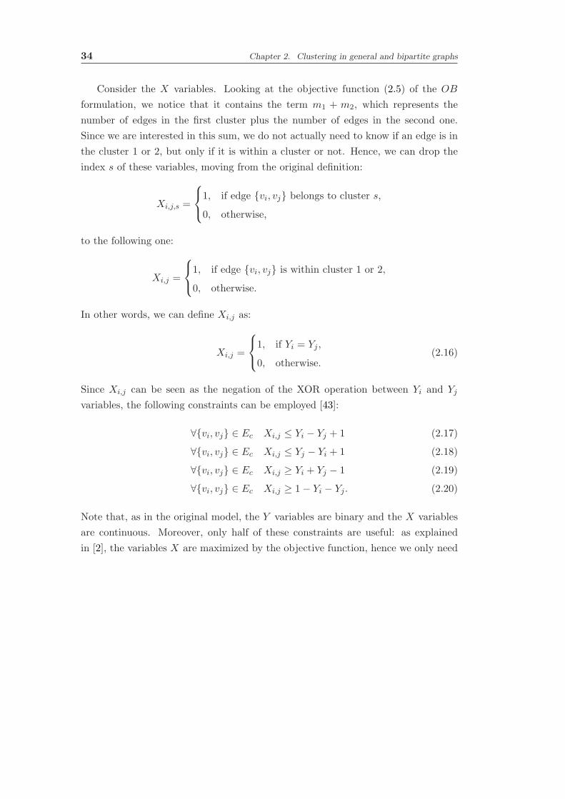
34 Chapter 2. Clustering in general and bipartite graphs
Consider the X variables. Looking at the objective function (2.5) of the OB
formulation, we notice that it contains the term m1 + m2, which represents the
number of edges in the first cluster plus the number of edges in the second one.
Since we are interested in this sum, we do not actually need to know if an edge is in
the cluster 1 or 2, but only if it is within a cluster or not. Hence, we can drop the
index s of these variables, moving from the original definition:
Xi,j,s =
1, if edge vi, vj belongs to cluster s,
0, otherwise,
to the following one:
Xi,j =
1, if edge vi, vj is within cluster 1 or 2,
0, otherwise.
In other words, we can define Xi,j as:
Xi,j =
1, if Yi = Yj ,
0, otherwise.(2.16)
Since Xi,j can be seen as the negation of the XOR operation between Yi and Yj
variables, the following constraints can be employed [43]:
∀vi, vj ∈ Ec Xi,j ≤ Yi − Yj + 1 (2.17)
∀vi, vj ∈ Ec Xi,j ≤ Yj − Yi + 1 (2.18)
∀vi, vj ∈ Ec Xi,j ≥ Yi + Yj − 1 (2.19)
∀vi, vj ∈ Ec Xi,j ≥ 1− Yi − Yj . (2.20)
Note that, as in the original model, the Y variables are binary and the X variables
are continuous. Moreover, only half of these constraints are useful: as explained
in [2], the variables X are maximized by the objective function, hence we only need

2.2. Clustering based on modularity maximization 35
(2.17)-(2.18). Therefore, we can reformulate the OB model this way:
max1
m
∑
vi,vj∈Ec
Xi,j −1
2m
(
D12 +
Dc2
2−D1Dc
)
(2.21)
s.t. ∀vi, vj ∈ Ec Xi,j ≤ Yi − Yj + 1 (2.22)
∀vi, vj ∈ Ec Xi,j ≤ Yj − Yi + 1 (2.23)
D1 =∑
vi∈Vc
kiYi (2.24)
D1 ∈ R (2.25)
∀vi ∈ Vc Yi ∈ 0, 1 (2.26)
∀vi, vj ∈ Ec Xi,j ∈ R. (2.27)
Due to the elimination of the index s from the variables X, their number is now
halved.
Consider again the definition (2.16) of the variables X. We can express it by
employing the product of the variables Yi and Yj this way:
Xi,j = 2YiYj − Yi − Yj + 1. (2.28)
Using this definition, we can replace the constraints (2.17)-(2.20) with a new set of
inequalities, and replace the variables X with another set of variables S (having the
same cardinality), which represent the product of the Y variables in (2.28). These
new variables S are defined as:
∀vi, vj ∈ Ec Si,j = YiYj ,
where the Fortet inequalities [93] can be used to describe this relationship (they can
be also obtained after applying (2.28) to (2.17)-(2.20)):
∀vi, vj ∈ Ec Si,j ≥ 0 (2.29)
∀vi, vj ∈ Ec Si,j ≥ Yj + Yi − 1 (2.30)
∀vi, vj ∈ Ec Si,j ≤ Yi (2.31)
∀vi, vj ∈ Ec Si,j ≤ Yj . (2.32)
We can now replace the variables X in the objective function (2.21) by means of
the equation (2.28), and we can replace the constraints (2.22)-(2.23) with the new
set (2.31)-(2.32) (again, we can drop the constraints (2.29) and (2.30) since we are
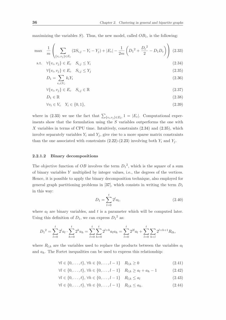
36 Chapter 2. Clustering in general and bipartite graphs
maximizing the variables S). Thus, the new model, called OB1, is the following:
max1
m
∑
vi,vj∈Ec
(2Si,j − Yi − Yj) + |Ec| −1
2m
(
D12 +
Dc2
2−D1Dc
)
(2.33)
s.t. ∀vi, vj ∈ Ec Si,j ≤ Yi (2.34)
∀vi, vj ∈ Ec Si,j ≤ Yj (2.35)
D1 =∑
vi∈Vc
kiYi (2.36)
∀vi, vj ∈ Ec Si,j ∈ R (2.37)
D1 ∈ R (2.38)
∀vi ∈ Vc Yi ∈ 0, 1, (2.39)
where in (2.33) we use the fact that∑
vi,vj∈EC1 = |Ec|. Computational exper-
iments show that the formulation using the S variables outperforms the one with
X variables in terms of CPU time. Intuitively, constraints (2.34) and (2.35), which
involve separately variables Yi and Yj , give rise to a more sparse matrix constraints
than the one associated with constraints (2.22)-(2.23) involving both Yi and Yj .
2.2.1.2 Binary decompositions
The objective function of OB involves the term D12, which is the square of a sum
of binary variables Y multiplied by integer values, i.e., the degrees of the vertices.
Hence, it is possible to apply the binary decomposition technique, also employed for
general graph partitioning problems in [37], which consists in writing the term D1
in this way:
D1 =
t∑
l=0
2lal, (2.40)
where al are binary variables, and t is a parameter which will be computed later.
Using this definition of D1, we can express D12 as:
D12 =
t∑
l=0
2lal ·t∑
h=0
2hah =t∑
l=0
t∑
h=0
2l+halah =t∑
l=0
22lal +t∑
l=0
∑
h<l
2l+h+1Rlh,
where Rl,h are the variables used to replace the products between the variables al
and ah. The Fortet inequalities can be used to express this relationship:
∀l ∈ 0, . . . , t, ∀h ∈ 0, . . . , l − 1 Rl,h ≥ 0 (2.41)
∀l ∈ 0, . . . , t, ∀h ∈ 0, . . . , l − 1 Rl,h ≥ al + ah − 1 (2.42)
∀l ∈ 0, . . . , t, ∀h ∈ 0, . . . , l − 1 Rl,h ≤ al (2.43)
∀l ∈ 0, . . . , t, ∀h ∈ 0, . . . , l − 1 Rl,h ≤ ah. (2.44)

2.2. Clustering based on modularity maximization 37
Again, as for constraints (2.29)-(2.32), only half of the inequalities have been ad-
joined. This time, since the variables R appear in the objective function with a
negative sign, we should add (2.41) and (2.42) to the model. Finally, to estimate the
parameter t of (2.40), recall that the maximum value which can be taken by D1 is
the sum of the degrees of all the vertices in the current cluster Dc. Moreover, from
(2.40) the maximum possible value for D1 is 2t+1− 1. Hence, t can be computed as:
2t+1 − 1 ≥ Dc ⇒ t = ⌈log2(Dc + 1)− 1⌉ . (2.45)
Now we can define the formulation OB2a:
max1
m
(
m1 +m2 −1
2m
(
t∑
l=0
22lal +
t∑
l=0
∑
h<l
2l+h+1Rlh +Dc
2
2−D1Dc
))
(2.46)
s.t. ∀vi, vj ∈ Ec Xi,j,1 ≤ Yi (2.47)
∀vi, vj ∈ Ec Xi,j,1 ≤ Yj (2.48)
∀vi, vj ∈ Ec Xi,j,2 ≤ 1− Yi (2.49)
∀vi, vj ∈ Ec Xi,j,2 ≤ 1− Yj (2.50)
∀l ∈ 0, . . . , t, ∀h ∈ 0, . . . , l − 1 Rl,h ≥ al + ah − 1 (2.51)
∀s ∈ 1, 2 ms =∑
vi,vj∈Ec
Xi,j,s (2.52)
D1 =∑
vi∈Vc
kiYi (2.53)
D1 =t∑
l=0
2lal (2.54)
∀s ∈ 1, 2 ms ∈ R (2.55)
D1 ∈ R (2.56)
∀vi ∈ Vc Yi ∈ 0, 1 (2.57)
∀l ∈ 0, . . . , t al ∈ 0, 1 (2.58)
∀vi, vj ∈ Ec, ∀s ∈ 1, 2 Xi,j,s ∈ R+0 (2.59)
∀l ∈ 0, . . . , t, ∀h ∈ 0, . . . , l − 1 Rl,h ∈ R+0 . (2.60)
Note that R+0 is the set of real numbers greater than or equal to 0, hence the
constraint (2.60) implies also (2.41).
Compact binary decomposition It is possible to reduce the number of variables
R in the previous model. The variable Rl,h is the linearization of the term alah, used
in the objective function (2.46). We can write the part of this objective function

38 Chapter 2. Clustering in general and bipartite graphs
which involves the variables Rl,h in this way:
t∑
l=0
∑
h<l
2l+h+1Rlh =t∑
l=0
∑
h<l
2l+h+1alah =t∑
l=0
2l+1al∑
h<l
2hah =
=t∑
l=0
2l+1albl =t∑
l=0
2l+1Rl,
(2.61)
where Rl = albl and bl is a new variable defined as∑
h<l 2hah. Since the upper
bound for bl is Ubl =∑
h<l 2h = 2l − 1, the constraints to add to the model are the
following (they are derived from the McCormick’s inequalities presented in Section
4.2.1.1):
∀l ∈ 0, . . . , t bl =∑
h<l
2hah (2.62)
∀l ∈ 0, . . . , t Rl ≥ 0 (2.63)
∀l ∈ 0, . . . , t Rl ≥ Ublal + bl − Ubl . (2.64)
With respect to the previous formulation, we have now replaced the t2+t2 variables
Rl,h with t + 1 variables Rl, and we have adjoined t + 1 variables b, and t + 1
constraints. Actually, we can notice that b0 = 0 and b1 = a0, but avoiding to define
these variables does not change significantly the computation time. More in general,
we can omit to define the variables b, since constraints (2.62) can be removed and
constraints (2.64) can be rewritten directly by replacing bl with∑
h<l 2hah. However,
for the sake of the clarity, and to ease the explanation of the formulation presented
in the following, we used the variables b. The formulation described in this section
is addressed as OB2b.
Second compact binary decomposition Consider again the objective function
(2.61) obtained after the transformation proposed in the previous section. In order to
have a more compact representation of it, we can put together the terms containing
the variables al and Rl in this way:
t∑
l=0
22lal +t∑
l=0
2l+1Rl =t∑
l=0
22lal +22l
2l−1Rl =
t∑
l=0
22l(
al +albl2l−1
)
.
Hence, we can write:
t∑
l=0
22l(
al +albl2l−1
)
=t∑
l=0
22l
2l−1al
(
bl + 2l−1)
=t∑
l=0
2l+1alzl =t∑
l=0
2l+1Tl,
where the new variable zl is equal to bl + 2l−1 and Tl is the linearization of alzl.
Then, we should remove the variables R and b from the OB2b formulation (and

2.2. Clustering based on modularity maximization 39
all the related constraints), and adjoin the new variables z and T , as well as these
constraints:
∀l ∈ 0, . . . , t zl =∑
h<l
2hah + 2l−1 (2.65)
∀l ∈ 0, . . . , t Tl ≥ 0 (2.66)
∀l ∈ 0, . . . , t Tl ≥ Uzlal + zl − Uzl , (2.67)
where Uzl is the upper bound of the variable zl, and it is equal to 2l− 1+ 2l−1. The
number of variables and constraints is the same as in the previous section (again,
we could omit to define z0 and z1, since z0 = 2−1 and z1 = a0 + 1, and we can omit
to define the variables z by expressing directly zl in the constraints (2.67) thanks to
equation (2.65)). The corresponding reformulation is called OB2c.
2.2.1.3 Symmetry breaking constraint
At each step of the algorithm a cluster is split into two new clusters, if this operation
has the effect to increase the modularity. It is easy to see that, given a solution,
the vertices in the first and second cluster can be swapped to obtain a symmetric
solution. Since the problem of the optimal bipartitioning is solved exactly by the
BB MIP algorithm of CPLEX, symmetric optima would lead to a large BB tree, and
as consequence the time to reach the leaves of the tree (i.e., the optimal solutions)
would increase. A simple way to avoid this is to fix one of the vertices to belong to
one of the clusters.
Some tests show that best results are obtained by fixing the vertex with highest
degree. Intuitively, this happens because that vertex is involved in more constraints.
Hence, the model OB3 is obtained by adding the following constraint to the model
OB:
Yg = 0, g = argmaxki, ∀vi ∈ Vc. (2.68)
Note that, in case of multiple vertices having the same maximum degree, we set g
to be the smaller among the indices of these vertices.
2.2.1.4 Numerical results
In this section we present the comparison of the numerical results provided by the
hierarchical divisive heuristic with the proposed reformulations. Results have been
obtained on a 2.8GHz Intel Core i7 CPU of a computer with 8 GB RAM running
Linux and CPLEX 12.2 [135], where we performed a fine tuning of the parameters
(more precisely, after some tests we found as best configuration the one where we dis-
abled the MIP cutting plane generation, and we used as branching variable selection
strategy the branch based on pseudo reduced costs). Results are obtained on a set of
instances of the literature, presented in Table 2.1. This set consists of these graphs:

40 Chapter 2. Clustering in general and bipartite graphs
Zachary’s karate club, describing friendship relationships in a karate club; Lusseau’s
dolphins, describing communications among a community of dolphins; Hugo’s Les
Miserables, representing relationships among characters in the book of Victor Hugo;
A00 main and A01 main, showing classes and relationships from a software project
related to graph drawing; p53, which shows protein interactions; Kreb’s political
books, representing books about US politics sold by Amazon; football, representing
scheduling of football matches between American college teams; USAir97, describing
connections between airports in the United States; netscience main, representing a
coauhtorship graph between scientists; s838, describing electronic circuits; power,
representing the topology of the power grid of the Western States of the United
States.
In Tables 2.2-2.4 we show the comparison of the performances of the divisive
hierarchical heuristic algorithm when the different proposed formulations for the
bipartition model are used. Nc denotes the number of clusters, Q the modularity,
and nodes the total number of BB nodes. Computing times are in seconds.
ID Graph n m Reference
1 karate 34 78 [251]2 dolphins 62 159 [175]3 Les miserables 77 254 [134,142]4 A00 main 83 135 [22]5 p53 protein 104 226 [71]6 political books 105 441 [22]7 football 115 613 [105]8 A01 main 249 635 [22]9 USAir97 332 2126 [22]10 netscience main 379 914 [196]11 s838 512 819 [190]12 power 4941 6594 [246]
Table 2.1: Informations about the graphs used for the tests.
It appears from Table 2.2 that the proposed reformulations of the original quadratic
model clearly impact the resolution time and the number of nodes of the BB tree.
OB1 outperforms OB3 in terms of computational time. As expected OB3 reduces
the number of BB nodes.
From Table 2.3 we note that when using the binary decomposition reformula-
tions we obtain the best computational time with the OB2c formulation (even if the
number of nodes is larger), except for some of the largest instances (i.e., 7 (football),
9 (USAir97), and 12 (power)) where the best one is OB2a. Note that slight discrep-
ancies may arise in the values of Nc and Q; they are due to the fact that optimal
bipartitions are not necessarily unique. For example, in the graph 6 (political books)
there are differences between the results obtained by the binary reformulations and
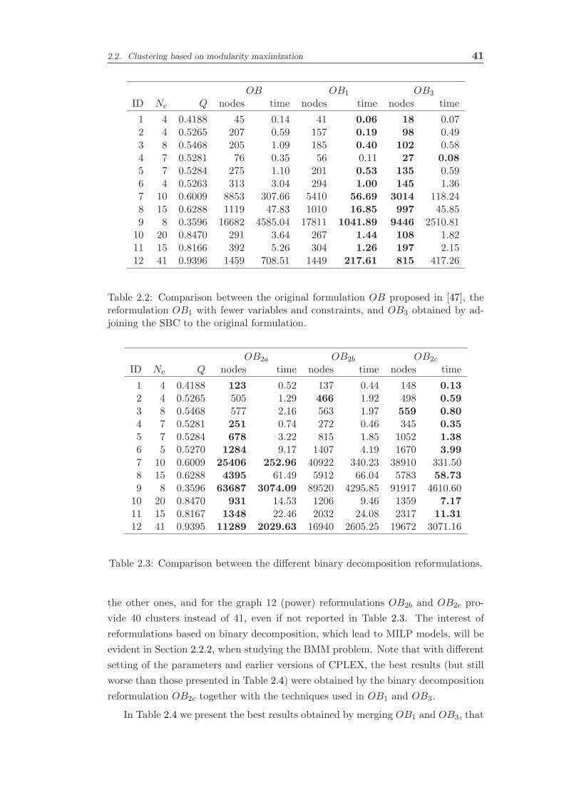
2.2. Clustering based on modularity maximization 41
OB OB1 OB3
ID Nc Q nodes time nodes time nodes time
1 4 0.4188 45 0.14 41 0.06 18 0.072 4 0.5265 207 0.59 157 0.19 98 0.493 8 0.5468 205 1.09 185 0.40 102 0.584 7 0.5281 76 0.35 56 0.11 27 0.085 7 0.5284 275 1.10 201 0.53 135 0.596 4 0.5263 313 3.04 294 1.00 145 1.367 10 0.6009 8853 307.66 5410 56.69 3014 118.248 15 0.6288 1119 47.83 1010 16.85 997 45.859 8 0.3596 16682 4585.04 17811 1041.89 9446 2510.8110 20 0.8470 291 3.64 267 1.44 108 1.8211 15 0.8166 392 5.26 304 1.26 197 2.1512 41 0.9396 1459 708.51 1449 217.61 815 417.26
Table 2.2: Comparison between the original formulation OB proposed in [47], thereformulation OB1 with fewer variables and constraints, and OB3 obtained by ad-joining the SBC to the original formulation.
OB2a OB2b OB2c
ID Nc Q nodes time nodes time nodes time
1 4 0.4188 123 0.52 137 0.44 148 0.132 4 0.5265 505 1.29 466 1.92 498 0.593 8 0.5468 577 2.16 563 1.97 559 0.804 7 0.5281 251 0.74 272 0.46 345 0.355 7 0.5284 678 3.22 815 1.85 1052 1.386 5 0.5270 1284 9.17 1407 4.19 1670 3.997 10 0.6009 25406 252.96 40922 340.23 38910 331.508 15 0.6288 4395 61.49 5912 66.04 5783 58.739 8 0.3596 63687 3074.09 89520 4295.85 91917 4610.6010 20 0.8470 931 14.53 1206 9.46 1359 7.1711 15 0.8167 1348 22.46 2032 24.08 2317 11.3112 41 0.9395 11289 2029.63 16940 2605.25 19672 3071.16
Table 2.3: Comparison between the different binary decomposition reformulations.
the other ones, and for the graph 12 (power) reformulations OB2b and OB2c pro-
vide 40 clusters instead of 41, even if not reported in Table 2.3. The interest of
reformulations based on binary decomposition, which lead to MILP models, will be
evident in Section 2.2.2, when studying the BMM problem. Note that with different
setting of the parameters and earlier versions of CPLEX, the best results (but still
worse than those presented in Table 2.4) were obtained by the binary decomposition
reformulation OB2c together with the techniques used in OB1 and OB3.
In Table 2.4 we present the best results obtained by merging OB1 and OB3, that

42 Chapter 2. Clustering in general and bipartite graphs
OB OB1 +OB3
ID Nc∗ Q∗ Nc Q nodes time nodes time
1 4 0.4198 4 0.4188 45 0.14 17 0.042 5 0.5285 4 0.5265 207 0.59 93 0.163 6 0.5600 8 0.5468 205 1.09 105 0.354 9 0.5309 7 0.5278 76 0.35 26 0.045 7 0.5351 7 0.5284 275 1.10 119 0.266 5 0.5272 4 0.5263 313 3.04 152 0.517 10 0.6046 10 0.6009 8853 307.56 3822 44.388 14 0.6329 15 0.6288 1119 47.83 726 9.729 6 0.3682 8 0.3596 16682 4585.04 8665 446.0610 19 0.8486 20 0.8470 291 3.64 94 0.8511 12 0.8194 15 0.8166 392 5.26 186 1.1812 - - 41 0.9396 1459 708.51 891 123.85
Table 2.4: Optimal solutions (Nc∗ and Q∗) obtained by the column generation ap-
proach presented in [10], and comparison between the results obtained by the originalformulation and the formulation OB1 with fewer variables and constraints, togetherwith the SBC of formulation OB3.
is the compact reformulation of the original quadratic model with SBC adjoined.
Both the computing time and the number of nodes are significantly reduced with
respect to the original formulation. The computing time is reduced by a factor up
to 10 for one of the largest instance, that is the number 9 (USAir97).
2.2.2 Extension to bipartite graphs
It is possible to extend the heuristic presented in previous section for the case of
bipartite graphs, where we want to maximize the bipartite modularity (2.2). As in
the previous case, the heuristic solves at each step a problem of optimal partitioning
where the number of clusters is equal to 2. We modify the best model obtained
for the unipartite case, namely the OB1 + OB3, adapting it for the bipartite case.
First at all, we should define some parameters and variables. The variables Y and
S, as well as parameters m and k, have the same meaning as for the MM problem.
Parameter Dc and variables D1 and D2 are no longer valid, thus we must modify
them. Since the first p vertices are red, and the other n−p vertices are blue, we can
define the two sets of blue and red vertices:
VRc = v1, . . . , vpVBc = vp+1, . . . , vn.
We should also define these two parameters:

2.2. Clustering based on modularity maximization 43
Rc =∑
vi∈VRc
ki (2.69)
Bc =∑
vj∈VBc
kj , (2.70)
which represent respectively the sum of the degrees of the red and blue vertices in
cluster c, and they are known before the bipartition. Moreover, we shall define the
following variables:
R1 =∑
vi∈VRc
kiYi (2.71)
B1 =∑
vj∈VBc
kjYj . (2.72)
Furthermore, the following relationships hold:
Rc = R1 +R2
Bc = B1 +B2.
The variables R1 and R2 represent, respectively, the sum of the degrees of the red
vertices in the clusters 1 and 2 obtained by splitting the cluster c, while B1 and B2
are the same quantities for blue vertices.
All these new parameters and variables are related to the corresponding ones of
MM by means of these relationships:
Vc = VRc ∪ VBc (2.73)
Dc = Rc +Bc (2.74)
D1 = R1 +B1. (2.75)
Since the number of clusters is 2, using the new variables and parameters intro-
duced above we can express the bipartite modularity (2.2) in this way:
Qbc =m1 +m2
m− R1B1 +R2B2
m2=m1 +m2
m− R1B1 + (Rc −R1) (Bc −B1)
m2=
=m1 +m2
m− 2R1B1 −BcR1 −RcB1 +RcBc
m2.

44 Chapter 2. Clustering in general and bipartite graphs
Hence, we can define the model BOB (Bipartite Optimal Bipartition) as:
max1
m
∑
vi,vj∈Ec
(2Si,j − Yi − Yj) + |Ec| −1
m(2R1B1 −BcR1 −RcB1 +RcBc)
(2.76)
s.t. ∀vi, vj ∈ Ec Si,j ≤ Yi (2.77)
∀vi, vj ∈ Ec Si,j ≤ Yj (2.78)
R1 =∑
vi∈VRc
kiYi (2.79)
B1 =∑
vj∈VBc
kjYj (2.80)
Yg = 1, g = argmaxki, ∀vi ∈ Vc (2.81)
R1 ∈ R (2.82)
B1 ∈ R (2.83)
∀vi, vj ∈ Ec Si,j ∈ R (2.84)
∀vi ∈ Vc Yi ∈ 0, 1. (2.85)
Note that the SBC (2.81) fix the variable Yg (associated to the vertex with the
largest degree) to 1, instead of 0 as done for MM in equation (2.68). Experiments
showed that this choice is more effective to break symmetries for bipartite graphs.
Looking at the objective function of the model, it is clear that it is not possible
to employ CPLEX, since we have now the product R1B1, and not a square as in the
unipartite case. Therefore, we have four possible ways to solve BOB:
1. employ general MINLP solvers, as Couenne or BARON;
2. linearize the products of binary variables Y arising from R1B1 using the Fortet
inequalities;
3. reformulate the problem in order to obtain a cMIQP model, and solve it with
CPLEX;
4. use the binary decomposition and then linearize the products appearing in the
resulting model.
As for MM it is too much time expensive to employ general MINLP solvers, so
this solution will not be considered.
2.2.2.1 Fortet linearization
Considering the linearization by means of the Fortet inequalities [93], we have to
replace the products between Y variables in R1B1 using a new set of variables W ,

2.2. Clustering based on modularity maximization 45
and to add some constraints. More precisely, the product R1B1 can be written as:
R1B1 =∑
vi∈VRc
kiYi∑
vj∈VBc
kjYj =∑
vi∈VRc
∑
vj∈VBc
kikjYiYj =∑
vi∈VRc
∑
vj∈VBc
kikjWi,j ,
where the variablesWi,j are defined by these constraints (again, since these variables
appear with negative sign inside an objective function to be maximized, only two
constraints are needed):
∀vi ∈ VRc , ∀vj ∈ VBc Wi,j ≥ 0
∀vi ∈ VRc , ∀vj ∈ VBc Wi,j ≥ Yi + Yj − 1.
Hence, we obtain the model BOB1a:
max1
m
∑
vi,vj∈Ec
(2Si,j − Yi − Yj) + |Ec| −1
m
2∑
vi∈VRc
∑
vj∈VBc
kikjWi,j+
−BcR1 −RcB1 +RcBc
(2.86)
s.t. ∀vi, vj ∈ Ec Si,j ≤ Yi (2.87)
∀vi, vj ∈ Ec Si,j ≤ Yj (2.88)
R1 =∑
vi∈VRc
kiYi (2.89)
B1 =∑
vj∈VBc
kjYj (2.90)
∀vi ∈ VRc , ∀vj ∈ VBc Wi,j ≥ Yi + Yj − 1 (2.91)
Yg = 1, g = argmaxki, ∀vi ∈ Vc (2.92)
R1 ∈ R (2.93)
B1 ∈ R (2.94)
∀vi, vj ∈ Ec Si,j ∈ R (2.95)
∀vi ∈ VRc , ∀vj ∈ VBc Wi,j ∈ R+0 (2.96)
∀vi ∈ Vc Yi ∈ 0, 1. (2.97)
Compact Fortet linearization Starting from the BOB1a model, it is possible
to obtain a more compact formulation. First, the objective function (2.86) can be
rewritten as:
1
m
∑
vi,vj∈Ec
(2Si,j − Yi − Yj + 1)− 1
m
∑
vi∈VRc
∑
vj∈VBc
kikj (2Wi,j − Yi − Yj + 1)
,

46 Chapter 2. Clustering in general and bipartite graphs
where the first and second part of the objective function present a similar structure.
Let ai,j be a parameter which is equal to 1 if there exists the edge vi, vj, and 0
otherwise. Moreover, let Hi,j be the parameter defined as:
∀vi ∈ VRc , ∀vj ∈ VBc Hi,j = ai,j −kikjm
.
We can define a compact model BOB1b as follows:
max1
m
∑
vi∈VRc
∑
vj∈VBc
Hi,j (2Wi,j − Yi − Yj + 1)
s.t. ∀vi ∈ VRc , ∀vj ∈ VBc : Hi,j < 0 Wi,j ≥ 0
∀vi ∈ VRc , ∀vj ∈ VBc : Hi,j < 0 Wi,j ≥ Yi + Yj − 1
∀vi ∈ VRc , ∀vj ∈ VBc : Hi,j > 0 Wi,j ≤ Yi∀vi ∈ VRc , ∀vj ∈ VBc : Hi,j > 0 Wi,j ≤ YjYg = 1, g = argmaxki, ∀vi ∈ Vc∀vi ∈ VRc , ∀vj ∈ VBc Wi,j ∈ R
∀vi ∈ Vc Yi ∈ 0, 1.
2.2.2.2 Square reformulation
It is possible to reformulate the BOB model to have only squares as nonlinearities
in the objective function, and use CPLEX as done for the unipartite case. Consider
this part of the objective function (2.76):
2R1B1 −BcR1 −RcB1. (2.98)
First at all, we can write the last two terms as:
BcR1 = (Bc +Rc)R1 −RcR1
RcB1 = (Bc +Rc)B1 −BcB1,
therefore we can rewrite (2.98) as:
2R1B1 − (Bc +Rc)(R1 +B1) +BcB1 +RcR1.
If we are able to introduce the terms B12 and R1
2, we can replace them and 2R1B1
with (R1 +B1)2. To do that, consider first the term RcR1. Using definitions (2.69)
and (2.71), we can write it this way:
RcR1 =∑
vi∈VRc
ki∑
vj∈VRc
kjYj =∑
vi∈VRc
ki2Yi +
∑
vi∈VRc
∑
vj∈VRc :j<i
kikj (Yi + Yj). (2.99)

2.2. Clustering based on modularity maximization 47
As stated earlier, we are interested in adding the term R12. We can express it as:
R12 =
∑
vi∈VRc
kiYi∑
vj∈VRc
kjYj =∑
vi∈VRc
ki2Yi +
∑
vi∈VRc
∑
vj∈VRc :j<i
2kikjYiYj , (2.100)
where we use the fact that Yi = Yi2, since Y are binary variables. Comparing (2.99)
and (2.100), it appears that we can write RcR1 in terms of R12 in this way:
R1Rc = R12 −
∑
vi∈VRc
∑
vj∈VRc :j<i
2kikjYiYj +∑
vi∈VRc
∑
vj∈VRc :j<i
kikj (Yi + Yj) =
= R12 +
∑
vi∈VRc
∑
vj∈VRc :j<i
kikj (Yi + Yj − 2YiYj) = R12+
+∑
vi∈VRc
∑
vj∈VRc :j<i
kikj (Yi − Yj)2.
We can obtain a similar result for the term B1Bc. More precisely, we can write:
B1Bc = B12 +
∑
vi∈VBc
∑
vj∈VBc :j<i
kikj (Yi − Yj)2.
Finally, equation (2.98) can be reformulated as:
2R1B1 − (Bc +Rc)(R1 +B1) +BcB1 +RcR1 = 2R1B1 − (Bc +Rc)(R1 +B1)+
+R12 +B1
2 +∑
vi∈VRc
∑
vj∈VRc :j<i
kikj (Yi − Yj)2 +∑
vi∈VBc
∑
vj∈VBc :j<i
kikj (Yi − Yj)2 =
= (R1 +B1)2 − (Bc +Rc)(R1 +B1) +
∑
vi∈VRc
∑
vj∈VRc :j<i
kikj (Yi − Yj)2+
+∑
vi∈VBc
∑
vj∈VBc :j<i
kikj (Yi − Yj)2.
Using relationships (2.73)-(2.75), we can now write the model BOB2. It is inter-
esting to notice that the objective function is similar to the objective function (2.33)
of the unipartite model OB1. More precisely, the first part of the objective function
is the same, as well as the terms D1 and −D1Dc. A first difference is the presence
of the term 1m, instead of 1
2m as in (2.33). Then, the term Dc2
2 is replaced by RcBc,
and there are the following additional terms:
∑
vi∈VRc
∑
vj∈VRc :j<i
kikj (Yi − Yj)2 +∑
vi∈VBc
∑
vj∈VBc :j<i
kikj (Yi − Yj)2.
Considering the set of constraints of the BOB2 model, it is exactly the same as that
of the model OB1, thus underlying the strong relationship between these problems.
The model BOB2 is defined as follows:

48 Chapter 2. Clustering in general and bipartite graphs
max1
m
∑
vi,vj∈Ec
(2Si,j − Yi − Yj) + |Ec| −1
m
(
D12 −D1Dc+
+∑
vi∈VRc
∑
vj∈VRc :j<i
kikj (Yi − Yj)2 +∑
vi∈VBc
∑
vj∈VBc :j<i
kikj (Yi − Yj)2 +RcBc
(2.101)
s.t. ∀vi, vj ∈ Ec Si,j ≤ Yj (2.102)
∀vi, vj ∈ Ec Si,j ≤ Yi (2.103)
D1 =∑
vi∈Vc
kiYi (2.104)
Yg = 1, g = argmaxki, ∀vi ∈ Vc (2.105)
∀vi, vj ∈ Ec Si,j ∈ R (2.106)
D1 ∈ R (2.107)
∀vi ∈ Vc Yi ∈ 0, 1. (2.108)
2.2.2.3 Binary decomposition
In order to linearize the term R1B1 we can employ the binary decomposition, simi-
larly as done for unipartite case. We can express the variables R1 and B1 as:
R1 =∑
vi∈VRc
kiYi =
tR∑
h=0
2hah (2.109)
B1 =∑
vj∈VBc
kjYj =
tB∑
l=0
2lbl, (2.110)
where ah and bl are binary variables, and the parameters tR and tB are defined,
similarly to equation (2.45), as:
2tR+1 − 1 ≥ Rc ⇒ tR = ⌈log2(Rc + 1)− 1⌉2tB+1 − 1 ≥ Bc ⇒ tB = ⌈log2(Bc + 1)− 1⌉ .
Using equations (2.109) and (2.110), we can express the product R1B1 in this way:
R1B1 =
tR∑
h=0
2hah
tB∑
l=0
2lbl =
tR∑
h=0
tB∑
l=0
2l+hahbl.
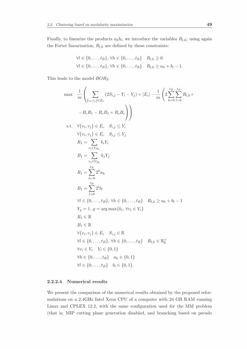
2.2. Clustering based on modularity maximization 49
Finally, to linearize the products ahbl, we introduce the variables Rl,h; using again
the Fortet linearization, Rl,h are defined by these constraints:
∀l ∈ 0, . . . , tB, ∀h ∈ 0, . . . , tR Rl,h ≥ 0
∀l ∈ 0, . . . , tB, ∀h ∈ 0, . . . , tR Rl,h ≥ ah + bl − 1.
This leads to the model BOB3:
max1
m
∑
vi,vj∈Ec
(2Si,j − Yi − Yj) + |Ec| −1
m
(
2
tR∑
h=0
tR∑
l=0
Rl,h+
−BcR1 −RcB1 +RcBc
s.t. ∀vi, vj ∈ Ec Si,j ≤ Yi∀vi, vj ∈ Ec Si,j ≤ YjR1 =
∑
vi∈VRc
kiYi
B1 =∑
vj∈VBc
kjYj
R1 =
tR∑
h=0
2hah
B1 =
tB∑
l=0
2lbl
∀l ∈ 0, . . . , tB, ∀h ∈ 0, . . . , tR Rl,h ≥ ah + bl − 1
Yg = 1, g = argmaxki, ∀vi ∈ VcR1 ∈ R
B1 ∈ R
∀vi, vj ∈ Ec Si,j ∈ R
∀l ∈ 0, . . . , tB, ∀h ∈ 0, . . . , tR Rl,h ∈ R+0
∀vi ∈ Vc Yi ∈ 0, 1∀h ∈ 0, . . . , tR ah ∈ 0, 1∀l ∈ 0, . . . , tB bl ∈ 0, 1.
2.2.2.4 Numerical results
We present the comparison of the numerical results obtained by the proposed refor-
mulations on a 2.4GHz Intel Xeon CPU of a computer with 24 GB RAM running
Linux and CPLEX 12.2, with the same configuration used for the MM problem
(that is, MIP cutting plane generation disabled, and branching based on pseudo

50 Chapter 2. Clustering in general and bipartite graphs
reduced costs). For bipartite case the instances described in the literature are not
numerous. We selected some bipartite graphs, presented in Table 2.5, from the Pa-
jek dataset [22]. The graphs are the following: Southern women, which represents
the attendance at 14 social event by 18 Southern women; Supreme court voting
represents the votes of 9 judges of the Supreme Court Justice on 26 important top-
ics on the years 2000-2001. The two graphs “yes” and “no” represent respectively
the votes yes and no of judges; social work is related to journals in the social work
citation graph, but no more informations are provided by Pajek; Wafa-CEO repre-
sents Galaskiewicz’s CEOs and clubs graph; divorces concerns 9 different causes of
divorces in the 50 States of the United States; Hollywood movies represents the rela-
tionships between 40 song composers and 62 film producers, where an edge between
the composer A and the producer B represents the fact that A created the sound-
track for a film produced by B; Scotland interlocks lists the 136 multiple directors
of the 108 largest joint stock companies in Scotland in 1904-1905; graph product
represents relationships between authors and papers taken from the bibliography of
the book [136] (note that this graph contains some disconnected components, since
m < n−1); network science has a structure similar to the previous graph, concerning
coautorship between scientists.
ID Graph p n m Reference
1 Southern women 18 32 89 [73]2 Supreme Court voting (yes) 26 35 147 [22]3 Supreme Court voting (no) 26 35 86 [22]4 social work 18 36 99 [22]5 Wafa - CEO 26 41 98 [245]6 divorces 50 59 225 [22]7 Hollywood movies 62 102 192 [85]8 Scotland interlocks 108 244 358 [224]9 graph product 314 674 613 [136]10 network science 960 2549 2580 [196]
Table 2.5: Informations about the graphs used in tests.
We now present the result obtained by the proposed formulations for the graphs
presented above. If CPLEX was not able to solve an instance because of memory
space overhead, we use the symbol “-”.
The first comparison is between the two models using the Fortet linearization,
namely BOB1a and BOB1b. Results presented in Table 2.6 clearly show that the
more compact formulation BOB1b outperforms the other one.
In Table 2.7 we present the results obtained by the best Fortet linearization
model BOB1b, the square formulation BOB2 and the binary decomposition for-
mulation BOB3. It appears that the square formulation is the worst, even if it
was the best choice for the MM problem. However, in that case there was only a

2.2. Clustering based on modularity maximization 51
BOB1a BOB1b
ID Nc Q nodes time nodes time
1 4 0.3409 437 0.30 72 0.192 2 0.2704 154 0.19 10 0.093 2 0.4538 45 0.14 6 0.074 5 0.2883 2169 1.46 1360 1.245 4 0.3329 1963 1.25 276 0.446 3 0.1876 1123 0.77 27 0.167 8 0.4939 1223370 4440.04 407104 3038.068 - - - - - -9 - - - - - -10 - - - - - -
Table 2.6: Comparison between the two Fortet reformulations.
square in the objective function (i.e., D12), whilst in the BOB2 model there are
many other squares. For small instances, the best choice is the model BOB1b. For
larger instances, the most suitable formulation is BOB3, which employs the binary
decomposition technique. In fact, the last three (largest) instances are solved only
by BOB3.
BOB1b BOB2 BOB3
ID Nc Q nodes time nodes time nodes time
1 4 0.3409 72 0.19 3372 1.32 670 0.392 2 0.2704 10 0.09 1074 1.39 618 0.433 2 0.4538 6 0.07 132 0.14 183 0.194 5 0.2883 1360 1.24 67364 13.11 1854 0.935 4 0.3329 276 0.44 117997 23.84 647 0.396 3 0.1876 27 0.16 2497924 646.78 2521 2.127 8 0.4939 407104 3038.06 - - 38910 5.268 13 0.7153 - - - - 3793 5.819 139 0.9363 - - - - 71927548 15450.4010 414 0.9696 - - - - 91917 38.49
Table 2.7: Comparison between the different reformulations.
Finally, we compare the quality of this divisive heuristic with respect to other
heuristics for the BMM problem. We report in Table 2.8 the results presented
in [171]. The results are available only for three graphs of Table 2.5, namely the
number 1 (Southern women), the number 8 (Scotland interlocks), and the number
10 (network science). However, in [171] tests are done with a version of the network
science graph with 2579 edges, whereas our version has 2580 edges.
It turns out that the best results are obtained by algorithm LPAb+ on these
instances. Our divisive heuristic obtains a worse result for the Southern women

52 Chapter 2. Clustering in general and bipartite graphs
Graph ID 1 Graph ID 8 Graph ID 10Algorithm Nc Q Nc Q Nc Q
Adaptive-BRIM 4 0.3455 13 0.6861 107 0.8894LPA-BRIM 4 0.3455 17 0.7141 500 0.9363CNM 3 0.3430 32 0.7008 414 0.9695MSG 3 0.3411 30 0.7004 414 0.9687LPAb 4 0.3192 60 0.5783 691 0.7808LPAb-MSG 4 0.3455 16 0.7194 414 0.9695LPAb+ 4 0.3455 16 0.7194 415 0.9696Divisive 4 0.3409 13 0.7153 414 0.9696
Table 2.8: Comparison between different heuristics for bipartite modularity maxi-mization on three instances: 1 (Southern women), 8 (Scoltand interlocks) and 10(network science).
graph. For Scotland interlocks, our modularity value is the second best one after
the value obtained by both LPAb-MSG and LPAb+. Finally, for network science
the value of modularity is equal to the one obtained by LPAb+. The results could be
improved by applying the split and merge technique recently presented in [48]. The
divisive heuristic is interesting in this context because it is a MP based approach.
However, even if the computational times are larger than those required by LPAb+,
the advantage is that it has not to be run many times as LPAb+.
2.3 Clustering based on strong and almost-strong con-
ditions
In this section we present a contribution which is not related to modularity maxi-
mization and MP in general. As stated at the beginning of this chapter, one of the
possible way to find communities in a graph consists of defining some conditions
which must be satisfied by all the communities.1 Among the best known conditions,
Radicchi et al. proposed the concept of community in the strong sense [210]:
Definition 2.3.1 (Community in the strong sense). A subset S of vertices of
a graph is called community in the strong sense if the number of neighbors of each
vertex within S is larger than the number of neighbors outside S.
Using the notation of indegree and outdegree presented in Section 2.1, we can
express this as ∀vi ∈ S kini > kouti , or equivalently, employing the adjacency matrix
notation, ∀vi ∈ S∑
vj∈S ai,j >∑
vj∈V \S ai,j . Note that the concept of defensive
alliance, studied in graph theory (see the thesis [225] and references therein), is
1Note that in this section we employ the term community instead of cluster, to be consistentwith the definitions proposed in the literature.

2.3. Clustering based on strong and almost-strong conditions 53
very close to that of community in the strong sense and is obtained by substituting
non-strict inequalities to strict ones.
We can also introduce the straightforward definition of partition in the strong
sense:
Definition 2.3.2 (Partition in the strong sense). A partition in the strong sense
consists only of communities in the strong sense.
However, the definition of strong community seems to be too stringent, in the
sense that a strong partition can be expected to contain only few communities, thus
resulting not informative. More precisely, the bigger problems are related to the
degree 2 vertices: following Definition 2.3.1, the two neighbors of a vertex having
degree 2 must belong to the same community, together with the vertex itself. If this
degree 2 vertex connects two heterogeneous communities, they could be merged in
a single, big community.
As a matter of fact, tests done with well-known graphs of literature support this
hypothesis. Therefore we introduce the concept of almost-strong community [44]:
Definition 2.3.3 (Community in the almost-strong sense). A subset S of
vertices of a graph is called community in the almost-strong sense if the number of
neighbors of each vertex within S is larger than the number of neighbors outside S,
except for the degree 2 vertices, where the number of neighbors within S can be larger
or equal to the number of neighbors outside S.
This means that all the vertices vi having degree 2 must satisfy the condition
kini ≥ kouti , and all the other vertices vt must satisfy the strong condition kint > koutt .
In other words, if a degree 2 vertex vi has two neighbors vj and vh, we have three
possibilities:
1. vi and vj belong to the same community, and vh to a different one;
2. vi and vh belong to the same community, and vj to a different one;
3. vi, vj and vh belong to the same community.
Note that the only case allowed by the definition of community in the strong
sense is the third one. We can now define the partition in the almost-strong sense:
Definition 2.3.4 (Partition in the almost-strong sense). A partition in the
almost-strong sense consists only of communities in the almost-strong sense.
It turns out that partitions in the almost-strong sense are more informative that
partitions in the strong sense, since all partitions in the strong sense are special cases
of partitions in the almost-strong sense. The following proposition formalizes this
fact:

54 Chapter 2. Clustering in general and bipartite graphs
Proposition 2.3.5 (Inclusion property). Let PS be the set of partitions in the
strong sense found for a given graph G = (V,E), and PA be the set of partitions in
the almost-strong sense found for the same graph. Then, PS ⊆ PA.
Proof. The only difference between communities in strong and almost-strong sense
is related to degree 2 vertices. From Definition 2.3.3, we have three possible ways
to assign a degree 2 vertex and its neighbors to communities, but only one of them,
namely the number 3, is compatible with the strong community definition. Thus,
PS is the set of partitions in the almost-strong sense where we always choice to put
each degree 2 vertex and its neighbors in the same community.
Another interesting property of the almost-strong communities is that if we merge
two of them, we obtain another valid almost-strong partition, as proved by the
following proposition:
Proposition 2.3.6 (Almost-strong merging property). Let P be a partition
in the almost-strong sense found for a given graph G = (V,E), consisting of the
almost-strong communities C1, C2, . . . , CM . Let P ′ be the partition composed by all
the communities of P except for two of them, namely Cj and Ck, which are replaced
by a new community Ci obtained by merging Cj and Ck. Then, P ′ is a partition in
the almost-strong sense.
Proof. Let vt be a vertex belonging to Cj or Ck, and then, after the merging, to
Ci. Let kint and koutt be respectively the indegree and outdegree of vt before the
merging, and kint′ , koutt′ be the same quantities after the merging. The consequence
of the merging is that the indegree of vt increases (or remains unchanged), whereas its
outdegree decreases (or remains unchanged). More precisely, the indegree increases,
and the outdegree decreases, if the vertex vt has some neighbors in the community
that will be merged with its own one. If vt has degree 2, the almost-strong condition
for partition P imposes that:
kint ≥ koutt .
It also holds, from the previous considerations:
kint′ ≥ kint ≥ koutt ≥ koutt′ .
Hence, the almost-strong condition for vt (i.e., kint′ ≥ koutt′ ) is also verified after the
merging. On the other hand, if vt has degree 6= 2, it holds that:
kint > koutt .
Again, from the previous considerations, we have:
kint′ ≥ kint > koutt ≥ koutt′ .

2.3. Clustering based on strong and almost-strong conditions 55
Hence, the almost-strong condition for vt (i.e., kint′ > koutt′ ) also holds when the degree
of vt is not 2. Since all the vertices in the new community Ci respect the almost-
strong condition and all the other communities remain unchanged, the partition P ′
is also an almost-strong partition.
The same property also holds for the strong partitions, as proved in the following
corollary:
Corollary 2.3.7 (Strong merging property). Proposition 2.3.6 is also valid for
strong partitions.
Proof. From Proposition 2.3.5, the strong partitions are a subset of the almost-strong
partitions. Thus, Proposition 2.3.6 is also valid if we consider strong partitions.
In the remainder of this section we introduce two MP model to describe the
problem of finding respectively partitions in the strong and almost-strong sense.
However, since these problems are too large to be solved efficiently, two algorithms
to enumerate respectively the partitions in the strong and almost-strong sense are
proposed, and then the results obtained with some well-known graphs of the litera-
ture are compared.
2.3.1 Strong communities detection
The problem of finding communities in the strong sense can be described by means
of a MILP model. Given a graph, let V be the set of n vertices, E the set of edges
and ki the degree of the vertex vi (as in the rest of the chapter). Moreover, P is
the set 1, . . . , n of indices of the communities (since we do not know how many
communities there are, but an upper bound is n, this set has cardinality n), Ct is the
variable equals to 1 if the community t contains at least one vertex and 0 otherwise,
and Zi,t is the binary variable equals to 1 if the vertex vi is inside the community

56 Chapter 2. Clustering in general and bipartite graphs
Ct. The MP model is the following:
max∑
t∈PCt (2.111)
s.t. ∀vi ∈ V∑
t∈PZi,t = 1 (2.112)
∀t ∈ P, ∀vj ∈ V∑
vi,vj∈EZi,t ≥ Zj,t
(⌊
kj2
⌋
+ 1
)
(2.113)
∀t ∈ P Ct ≤∑
vi∈VZi,t (2.114)
∀t ∈ P : t < n Ct ≤ Ct+1 (2.115)
∀t ∈ P Ct ≤ 1 (2.116)
∀t ∈ P Ct ∈ R (2.117)
∀vi ∈ V, ∀t ∈ P Zi,t ∈ 0, 1, (2.118)
where the objective function (2.111) aims at maximizing the number of commu-
nities, the constraints (2.112) force each vertex to belong to only one community,
the constraints (2.113) express the strong condition for the vertex vj belonging to
the community t, the constraints (2.114) fix to 1 the variable Ct if there is at least
one vertex in the community t, 0 otherwise (this holds because these variables are
maximized by the objective function). Note that the variables C do not need to be
defined as binary, but only smaller than or equal to 1 (see constraints (2.116)). The
constraints (2.115) are SBCs used to impose that the communities non-empty are
the ones having bigger index (these kind of lexicographic order SBCs are presented
in detail in the next chapter, in Section 3.3.2). The main problem of this formu-
lation is that there are n2 binary variables Z. A formulation having O(n2) binary
variables can be only solved for small instances. This is the reason why we design
a specific algorithm to find partitions in the strong sense (actually, the definition of
MP models to describe strong and almost-strong rules is a work in progress with
Cafieri, Caporossi, Hansen, and Perron). In fact we present an algorithm, called SC
(Strong Communities), to enumerate all the partitions in strong sense for a given
graph G = (V,E).
Note that this problem always has a solution, i.e., the trivial partition consisting
in a single community containing all the vertices. The algorithm will make use of
two types of labels associated with the vertices and the edges of G respectively: label
li associated with vertex vi, i = 1, . . . , n (initially li = i for all vertices, and at the
current iteration the label of the vertex vi is equal to the smallest label of a vertex of
the community to which vi belongs); the label ti,j associated with edge vi, vj cantake three values (−1, 0, 1). It is equal to -1 if it has already been decided that the
vertices vi and vj belong to different communities; it is equal to 1 if it has already
been decided that vertices vi and vj belong to the same community. If no decision

2.3. Clustering based on strong and almost-strong conditions 57
has been taken, ti,j = 0. The rules of this algorithm are the following:
• Rule 1 (pending edges): if the edge vi, vj is a pending one, set its label ti,j
to 1 and set both li and lj to min(li, lj). In words, both vertices of a pending
edge must belong to the same community.
• Rule 2 (degree two vertices): if vertex vi has degree ki = 2, and its neighbors
are vj and vk, set ti,j = 1, ti,k = 1 and li = lj = lk = min(li, lj , lk). In words,
if a vertex vi has degree 2 and neighbors vj and vk, it follows from the strong
condition that all three vertices vi, vj , vk must belong to the same community.
Note that the Rules 1 and 2 should be applied only once, at the beginning of
the resolution. Moreover, the order of selection of the vertices for Rule 2 does not
change the communities found (regardless of the labels for each community).
• Rule 3.a (positive transitivity): if li = lj and ti,j = 0, set ti,j = 1. In words,
if two vertices vi and vj belong to the same community, and are joined by an
edge which does not specify that, set the label of this edge as positive.
• Rule 3.b (negative transitivity): if li 6= lj and ti,j = −1, set ta,b = −1 ∀va, vb :la = li, lb = lj , and ta,b = 0. In words, if two vertices belong to different
communities and are joined by a negative edge, set to -1 all the edges with
label 0 joining two vertices of these communities.
• Rule 4.a (majority 1 ): if the majority of neighbors of the vertex vi belong to
the same community and the label of the vertices belonging to this community
is l, set li = l = min(l, li) and apply the positive transitivity Rule. In words,
if half or more of the neighbors of vi have the same label l, the only way to
satisfy the strict inequality of the strong condition is to add the vertex vi to
the community where its vertices have label l.
• Rule 4.b (majority 2 ): if a vertex vi has degree ki = 2d, and there are d
neighbors with label l1 and d neighbors with label l2, set li = min(l1, l2), and
for all the vertices vk with lk = l1 or lk = l2, set lk = li. Then, apply the
positive transitivity Rule. In other words, we merge the communities with
labels l1 and l2, and we put in this new community the vertex vi, too.
• Rule 4.c (majority 3 ): if the number of negative edges, i.e., edges labeled with
-1, incident with the vertex vi is equal to⌈
ki2
⌉
−1, for all the neighbor vertices
vj of vi having ti,j = 0, set ti,j = 1, and for all the vertices vk with lk = lj , set
lk = li. In words, when the number of negative edges incident to vi is almost
the majority there is only one way to satisfy the strong condition at vertex vi,
i.e., set the label associated to all other incident edges to 1.
Rules 3 and 4 must be repeated as long as there is at least one change of label.

58 Chapter 2. Clustering in general and bipartite graphs
• Rule 5 (branching): if no more labels of edges can be modified according to
the previous rules, select an edge with label 0 which joins the two largest
communities. Set the label of this edge to -1 (left branch), then set separately
this label to 1 (right branch). The application of Rule 5 so generates always
two subproblems of the current problem, corresponding respectively to label
-1 and label 1 for the selected edge. The two subproblems are stored and
the algorithm proceeds returning to Rule 3.a to process each of the stored
subproblems (one at a time).
• Rule 6.a (no majority): if the number of negative edges incident with the
vertex vi is larger than⌈
ki2
⌉
− 1, apply Rule 8 below.
• Rule 6.b (no coherent labels): if there exist two vertices vi and vj with li = lj
and ti,j = −1, apply Rule 8 below.
• Rule 7 (feasible solution): if all edges have a label -1 or 1, store the corre-
sponding partition, then apply Rule 8.
• Rule 8 (backtracking): return to the latest application of the branching rule
and consider the right hand-side branch as current subproblem.
2.3.2 Almost-strong communities detection
As done for partitions in the strong sense, this problem can be described as a MILP:
max∑
t∈PCt (2.119)
s.t. ∀vi ∈ V∑
t∈PZi,t = 1 (2.120)
∀t ∈ P, ∀vj ∈ V : kj 6= 2∑
vi,vj∈EZi,t ≥ Zj,t
(⌊
kj2
⌋
+ 1
)
(2.121)
∀t ∈ P, ∀vj ∈ V : kj = 2∑
vi,vj∈EZi,t ≥ Zj,t (2.122)
∀t ∈ P Ct ≤∑
vi∈VZi,t (2.123)
∀t ∈ P : t < n Ct ≤ Ct+1 (2.124)
∀t ∈ P Ct ≤ 1 (2.125)
∀t ∈ P Ct ∈ R (2.126)
∀vi ∈ V, ∀t ∈ P Zi,t ∈ 0, 1, (2.127)
where the difference is the modification of the strong conditions (2.113): these con-
ditions continue to hold for vertices having degree different to 2 (see constraints
(2.121)), but the almost-strong version is introduced for vertices having degree 2

2.3. Clustering based on strong and almost-strong conditions 59
(see constraints (2.122)). Comparing the almost-strong formulations (2.119)-(2.127)
with the strong formulation (2.111)-(2.118) we notice that the almost-strong formu-
lation is a relaxation (using the terminology introduced in Section 1.3.1.3) of the
strong one, since the constraint (2.113) is relaxed for the vertices having degree two.
Hence, the feasible region can be larger and the optimal solution of the almost-strong
formulation is an upper bound on the optimal solution of the strong formulation,
since these are maximization problems. This is a “mathematical programming” ex-
planation of the fact that the partitions in the almost-strong sense can have a larger
number of communities, that is a consequence of Proposition 2.3.5. Again, this
problem is hard to solve, and we propose an enumerative algorithm to solve it in the
following.
In fact, in order to find all the partitions in almost-strong sense, we modify the
algorithm presented in the previous section and we adapt it to the Definition 2.3.3.
Rules of this algorithm, called ASC (Almost-Strong Communities) are the following:
• Rule 1 (pending edges): if the edge vi, vj is a pending one, set its label ti,j
to 1 and set both li and lj to min(li, lj). In words, both vertices of pending
edge must belong to the same community.
Note that the Rule 1 should be applied only once, at the beginning of the res-
olution. Rule 2 of SC algorithm has been removed due to considerations presented
after Definition 2.3.3.
• Rule 3.a (positive transitivity): if li = lj and ti,j = 0, set ti,j = 1. In words,
if two vertices vi and vj belong to the same community, and are joined by an
edge which does not specify that, set the label of this edge as positive.
• Rule 3.b (negative transitivity): if li 6= lj and ti,j = −1, set ta,b = −1 ∀va, vb :la = li, lb = lj , and ta,b = 0. In words, if two vertices belong to different
communities and are joined by a negative edge, set to -1 all the edges with
label 0 joining two vertices of these communities.
• Rule 4.a.1 (majority 1 ): if the majority of neighbors of the vertex vi with
ki 6= 2 belong to the same community and the label of the vertices belonging
to this community is l, set li = l = min(l, l1) and apply the positive transitivity
Rule.
• Rule 4.a.2 (majority 1’ ): if both neighbors of the vertex vi with ki = 2 belong to
the same community and the label of the vertices belonging to this community
is l, set li = l = min(l, l1) and apply the positive transitivity Rule.
• Rule 4.b (majority 2 ): if a vertex vi has degree ki = 2d 6= 2, and there are d
neighbors with label l1 and d neighbors with label l2, set li = min(l1, l2), and
for all the vertices vk with lk = l1 or l2, set lk = li. Then, apply the positive

60 Chapter 2. Clustering in general and bipartite graphs
transitivity Rule. In other words, merge the communities with labels l1 and
l2, and put in this new community the vertex vi, too.
• Rule 4.c.1 (majority 3 ): if the number of negative edges incident with the
vertex vi with degree ki 6= 2 is equal to⌈
ki2
⌉
− 1, for all the neighbor vertices
vj of vi having ti,j = 0, set ti,j = 1, and for all the vertices vk with lk = lj , set
lk = li.
• Rule 4.c.2 (majority 3’ ): if the number of negative edges incident with the
vertex vi with degree ki = 2 is equal to 1, for all the neighbor vertices vj of vi
having ti,j = 0, set ti,j = 1, and for all the vertices vk with lk = lj , set lk = li.
Rules 3 and 4 must be repeated as long as there is at least one change of label.
• Rule 5 (branching): if no more labels of edges can be modified according
to the previous rules, select an edge with label 0 which joins the two largest
communities. Set the label of this edge to -1 (left branch). Then set separately
this label to 1 (right branch), store the current subproblem, and return to Rule
3.a.
• Rule 6.a.1 (no majority): if the number of negative edges incident with a vertex
vi with degree ki 6= 2 is larger than⌈
ki2
⌉
− 1, apply Rule 8 below.
• Rule 6.a.2 (no majority’ ): if the number of negative edges incident with a
vertex vi with degree ki = 2 is larger than 1, apply Rule 8 below.
• Rule 6.b (no coherent labels): if there exist two vertices vi and vj with li = lj
and ti,j = −1, apply Rule 8 below.
• Rule 7 (feasible solution): if all edges have a label -1 or 1, store the corre-
sponding partition, then apply Rule 8.
• Rule 8 (backtracking): return to the latest application of the branching rule
and consider the right hand-side branch as current subproblem.
2.3.3 Comparison between SC and ASC
We compare the results obtained by the two algorithms SC and ASC for 4 graphs.
The vertices belonging to the same community are represented with the same shape
and color in the figures. Since the partitions in the almost-strong sense can be
numerous, we only consider those with the largest number of communities. Note
that the trivial partition with a single cluster containing all the vertices is found by
both SC and ASC.
The first graph considered is Zachary’s karate club [251]. It consists of 34 vertices
associated to the members of a karate club, while edges represents friendship rela-
tionships between these members after a split due to a dispute between the karate
club administrator and the instructor.

2.3. Clustering based on strong and almost-strong conditions 61
The split observed by Zachary leads to the communities C1 = 1, 2, 3, 4, 5, 6, 7, 8,10, 11, 12, 13, 14, 17, 18, 20, 22 and C2 = V \C1. The SC algorithm finds only the
trivial partition and the one presented in Figure 2.2(a), while ASC finds the par-
tition presented in Figure 2.2(b), and other 22 partitions into two communities.
In particular one of these partitions, obtained by merging the diamond and circle
shaped communities (see Proposition 2.3.6), is the partition found by Zachary.
(a) (b)
Figure 2.2: Partitions into strong and almost-strong communities obtained by algo-rithms SC and ASC respectively for Zachary karate club graph.
The second graph concerns informal communications within a sawmill on strike
[189]. Vertices are associated with the 24 employees of a wood processing facility
where a new management team proposes changes to the compensation package. The
workers refuse and a strike follows. Facing a stalemate, the management asks a con-
sultant to analyze the communications among the employees. Edges of the graph cor-
respond to frequent discussions on the strike between pairs of colleagues. Two par-
titions into strong communities were obtained with the SC algorithm; one of them,
represented in Figure 2.3(a), is composed of a first community C1 = 10, 11, 12, 13corresponding to all Spanish-speaking employees, and another one representing 20
employees who are English-speaking. The ASC algorithm gives 20 partitions. A
single one of them has 4 communities (see Figure 2.3(b)), and none had more. The
small community with 4 Spanish-speaking employees remains the same. The second
community of 20 employees is split into 3 communities: a first one corresponds to
9 English-speaking employees with age smaller than or equal to 30. The second
community with 9 employees and the third one with 2 employees correspond to
older English-speaking workers. The partition of the 24 employees in three commu-
nities, i.e., Spanish-speaking, young English-speaking, and older English-speaking
employees obtained by joining the two last communities corresponds exactly to the
partition obtained by the consultant. As the strong conditions and the almost-strong
conditions remain satisfied when communities are merged (due to Proposition 2.3.6
and Corollary 2.3.7), the ASC algorithm did also find the optimal three community

62 Chapter 2. Clustering in general and bipartite graphs
partition. Detection of the small community with employees 16 and 21 may be in-
terpreted in that these employees are less talkative, or less concerned by the strike,
than most of the others.
It thus appears that algorithm SC recognizes well a small, almost isolated com-
munity but groups unduly the others. Algorithm ASC finds the optimal partition
and it perhaps provides a little more information. Note the importance of vertex 15
having degree 2.
(a) (b)
Figure 2.3: Partitions into strong and almost-strong communities obtained by algo-rithms SC and ASC respectively for the strike graph.
A next example is a directed graph representing a glossary of graphs and di-
graphs, which can be found in the Pajek repository [22]. An arc from vi to vj means
that the concept associated with vi is used in the definition of vj . We neglected
orientation of arcs and considered only the largest connected component, which has
60 vertices and 114 edges. Applying algorithm SC only the trivial partition was
found. Turning to algorithm ASC, many partitions were obtained, 5 of which have
the largest number of communities, i.e., 6. The most intuitively appealing of them
is presented on Figure 2.4. We next comment on these communities going from
the smallest to the largest. The first community corresponds to two terms, i.e.,
complete, clique. They are clearly close, as a complete graph is a clique. The
second community also has two terms, pertained to computer search, i.e., child,ordered tree. These two communities appeared unchanged in all 5 partitions into
6 communities. A third community contains 7 terms, i.e., decision tree, binary
search tree, m-ary tree, rooted tree, offspring, level, height. All those terms cor-
respond, as did those of community 2, to computer search. Community three is
similar in the 4 other partitions into 6 communities except for that the term deci-
sion tree is assigned to another community. A fourth community contains 8 terms,
i.e., diameter, distance, hamiltonian, walk, trail, path, acyclic graph, cycle. Theseterms correspond to concepts related to paths and cycles. A fifth community con-
tains 17 terms, i.e., strongly connected, tournament, digraph, orientation, arc list,

2.3. Clustering based on strong and almost-strong conditions 63
Figure 2.4: Partition into almost-strong communities obtained by algorithm ASCfor the graph and digraph glossary graph.
neighborhood, node, order, internal vertex, vertex, pendant vertex, leaf, degree,
regular, adjacency structure, adjacent, closure. It seems difficult to find a concept
encompassing all of these terms. The five first, i.e., strongly connected, tournament,
digraph, orientation, arc list correspond to oriented graphs. The remainder corre-
sponds to vertices and adjacency. Note that this community contains several pairs
of synonyms, i.e., node and vertex, and pendant vertex and leaf. The sixthcommunity contains 24 terms, i.e., label, isomorphic, planar, edge, size, topological
order, adjacency matrix, loop, reduced graph, condensed graph, homeomorphic, bi-
partite graph, spanning subgraph, subgraph, spanning tree, connected component,
bridge, connected, forest, tree, graph, cromatic number, k-colorable, arc. This
community appears to be less homogeneous than the others. Some concepts are
related to edges, i.e., edge, loop, size, label. Others correspond to properties or
families of graphs: isomorphic, homeomorphic, condensed graph, reduced graph,
bipartite graph, spanning subgraph, spanning tree, subgraph, connected component,
connected, bridge, tree, k-colorable, cromatic number, graph. Although this par-
tition appears to be quite informative, it is not perfect, e.g., because forest and
acyclic graph are synonyms but attributed to different communities. Or yet close
terms such as adjacency matrix and adjacency structure are also attributed to
different communities.
A fourth example comes from the well-known paper on dolphins due to Lusseau
et al. [175]. However, it does not concern the set of all 62 dolphins, but another graph
giving the sociogram of the community for groups followed between 1995 and 2001.

64 Chapter 2. Clustering in general and bipartite graphs
This graph has 40 vertices and 70 edges. When trying to find communities in the
strong sense four partitions were obtained, one with three communities, represented
on Figure 2.5(a), two obtained by merging pairs of adjacent communities, and the
trivial partition.
(a) (b)
Figure 2.5: Partitions into strong and almost-strong communities obtained by algo-rithms SC and ASC respectively for the small dolphin graph.
Finding communities in the almost-strong sense gives a partition in eight com-
munities, which is represented in Figure 2.5(b). It refines one of the communities
by isolating a small two vertices community with one vertex of degree two. It also
refines more drastically the largest community by isolating four subgraphs with two,
two, three, and four entities. Each of these subgraphs contains a vertex of degree
two. It appears clearly that this almost-strong partition is more informative than
any other strong one.
2.4 Conclusions
In this chapter the problem of clustering in general and bipartite graphs is studied,
and some techniques for finding good quality partitions are proposed. More precisely,
we focus on modularity, and on some conditions which must be respected by each
cluster.
In the fist part, we proposed some reformulations for the MP model used by a
hierarchical divisive heuristic. Tests showed that the best results are obtained by
means of a cMIQP model together with a SBC. As a matter of fact, we can employ
CPLEX as solver, since the objective function is convex (the square variable has a
negative coefficient in the objective function, and it is a maximization problem). We
also presented some reformulations based on binary decomposition techniques for

2.4. Conclusions 65
integer variables, which are not very efficient. However, this method has been intro-
duced because it is the best choice for bipartite modularity maximization problem.
Using general MINLP solvers, as well as applying directly Fortet inequalities was
not considered, because too much time consuming.
We then considered the problem of maximizing bipartite modularity. First, we
adapt the divisive heuristic for bipartite graphs. The original formulation used
by the heuristic cannot be solved by CPLEX. Thus, starting from our knowledge
on the previous case, we proposed some reformulations, i.e., a model presenting a
convex objective function with squares, another one based on Fortet linearization
(and starting from it, a more compact version), and a model which employs binary
decompositions. In this case, the formulation with squares was the worst. This
difference with respect to the unipartite case is due to the fact that for the bipartite
case there are several squares in the objective function, whereas in the unipartite case
there is only one square. For small instances the compact version of the model based
on Fortet inequalities is the best, while the model based on the binary decomposition
outperforms the former for larger instances. Indeed, the techniques employed in the
unipartite case to obtain a more compact formulation and the SBC were employed
as well.
Hence, for similar problems the best MP formulation can be different, and based
on techniques which do not perform well in the other case. It is interesting to notice
that the proposed reformulations are exact formulations of the original problem,
because Fortet-based linearization for binary problem are exact. This is also showed
in Chapter 4. Actually, we introduce a simple but effective SBC, thus obtaining a
narrowing. However, the study of narrowings will be the subject of Chapter 3.
In the last part of the thesis, we analyzed clustering from another point of view,
that is by means of some rules defined for each cluster. Starting from the existing
strong conditions, we relax them obtaining the almost-strong conditions, which give
more informative partitions. Even if this part is not strictly related with reformu-
lations, it represents another interesting approach for clustering problems. We first
proposed MP formulations for the problems of finding partitions in the strong and
almost-strong sense. Since the corresponding formulations are too large (in terms
of binary variables) we proposed two enumerative algorithms to find these parti-
tions. Adapting the terminology used for reformulations, we could say that the MP
formulation associated to the almost-strong conditions is a relaxation of that one
associated to the strong conditions, as it provides better results in terms of number
of communities found, that is the objective function to maximize (as a relaxation
provides usually an equal or better optimal solution with respect to the original
problem) and the partitions obtained with the strong conditions are a subset of the
partitions in the almost-strong sense (as a relaxation can have a larger feasible re-
gion with respect to the original problem). The study of relaxations is the topic of
Chapter 4.

66 Chapter 2. Clustering in general and bipartite graphs

Part II
An application of narrowings


69
Circle packing in a square is a well-known problem in mathematics, with several
applications. It is possible to describe it by means of MP, obtaining a NLP problem.
However, due to its complexity, many approaches presented in the literature are
heuristics. An interesting feature of the problem of packing equal circles in a square
(PECS) is that it involves a high degree of symmetry, making it a good candidate for
the application of narrowing reformulations. In this part of the thesis we first present
the problem and some MP formulations to describe it. Then we characterize its
symmetries, and we introduce some Symmetry Breaking Constraints (SBCs), which
lead to narrowings, to break these symmetries, as well as some other constraints that
improve the formulations. We compare the narrowings to the original formulation,
showing that the former outperform the latter in terms of both computational time
and size of the BB tree. We also propose a conjecture about the reduction of
the range for some of the variables of the problem. This chapter is based on the
papers [59–61,63, 64]. The full proof of Theorem 3.4.2 is unpublished.

70
Chapter 3Circle packing in a square
Circle packing is a classical problem in mathematics [233,237]. Applications include
cutting problems (cut out as many identical disks as possible from a piece of mate-
rial) [66, 126, 128], container loading (place as many identical cylindrical objects as
possible into a container) [99,103], and tree reforestation, where the aim is to plant
trees (which grow approximately at the same speed) in a given region maximizing
both their density and size. In this chapter we consider the problem of packing equal
circles in a square having side-length 1. For an application-oriented survey see [52].
Circle packing in a square can be casted in form of optimization or decision
problem. Moreover, there exist different but equivalent formulations for the problem
itself: if an optimum for one of these is known, then we can easily find the optimal
solutions for the others. Among the most known settings for the optimization version
of this problem, we have the following:
Packing Equal Circles in a Square (PECS). Given an integer
n > 0, find the maximum common radius r for n non-overlapping cir-
cles arranged in the unit square.
Point Packing in a Square (PPS). Given an integer n > 0, place n
points in the unit square such that their minimum pairwise distance m
is maximized.
Usually the PPS problem is stated in an alternative but equivalent way (details
are provided in Section 3.1):
Point Packing in a Square (PPS). Given an integer n > 0, place
n points in the unit square such that their squared minimum pairwise
distance α is maximized.
The corresponding decision formulations of these problems are:

72 Chapter 3. Circle packing in a square
Decision version of PECS. Given an integer n > 0 and a radius r > 0,
can n circles of radius r be packed in a unit square in such a way that
the interiors of the circles have pairwise empty intersection?
Decision version of PPS. Given an integer n > 0 and a rational α ≥ 0,
can n points be determined in the unit square in such a way that their
squared minimum pairwise distance is greater than or equal to α?
In order to show the correspondence between PPS and PECS, here is a reduction
from PPS to PECS: (a) every NO instance of the PPS problem is a NO instance of the
PECS problem; (b) if a YES instance of the PPS problem is such that r ≥√α
2+2√αthen
it is also a YES instance of the PECS problem (the inequality can be verified easily
by scaling the PPS configuration down so that it allows enough space to arrange
circles wholly contained within the square); (c) otherwise, it is a NO instance of the
PECS problem (Chapter 2 in [237]). Thus, given an instance of the PPS problem
with its YES/NO decision, a YES/NO decision can be taken in constant time for the
PECS problem. A similar transformation from PECS to PPS also holds. A graphical
representation of the relationship between PECS and PPS is given in Figure 3.1.
Figure 3.1: Optimal solutions of PECS and PPS for the instance where n = 10. Thepicture is taken from [235].
The exact formula expressing the relationship existing between the radius rn of
PECS and the distance mn of PPS when the number of circles (points) is n is the
following [237]:
mn =2rn
1− 2rn.
There exist also theoretical bounds on the optimal radius r∗n of PECS and the optimal
distance m∗n of PPS, as reported in [237]:
Definition 3.0.1 (Bounds on the distance). For each n ≥ 2 integer, it holds
that:√
2√3n≤ m∗
n ≤1
n− 1+
√
1
(n− 1)2+
2√3(n− 1)
.

73
Definition 3.0.2 (Bound on the radius). For each n ≥ 2 integer, it holds that:
r∗n ≤ min
1√
2√3n+ 4 (⌊√n⌋ − 2)
(
2−√3)
,1 +
√
1 + 2√3(n− 1)
2n+ 2√
1 + 2√3(n− 1)
.
A different decision version of the problem, where radius is fixed and the side of
the square is a parameter, is the following:
Given a rational S > 2 and an integer n > 0, can n non-overlapping
circles of radius 1 be arranged in a square of side S?
In this thesis we consider PECS and PPS (their optimization version). Their
MP formulations are presented in details in Section 3.1. For more details about the
existing formulations for this problem, see [237].
Complexity The PECS problem belongs to at least two classes of NP-hard prob-
lems: the Quadratically Constrained Quadratic Problem (QCQP) [243]
and the Circle Packing Problem (CPP), where one is given a sequence of n
radii r1, . . . , rn and must decide whether n circles with respective radii can fit in
a unit square; the CPP was recently shown to be NP-hard [75]. The proof em-
ploys different radii and therefore does not seem applicable to PECS. Because the
YES-certificates of PECS instances might involve irrational numbers, it is unclear
whether PECS is in NP.
Let (r1, . . . , rn) be a YES instance of the CPP, and C = ((xi, yi) | i ≤ n) be a
certificate (i.e., the sequence of circle centers). The coin graph of C is an undirected
graph G = (V,E) such that V = 1, . . . , n and for all u, v ∈ V we have (u, v) ∈ Eif√
(xu − xv)2 + (yu − yv)2 = ru + rv. It is known that a graph is a coin graph if
and only if it is finite, simple, and planar [219]. Determining whether a given graph
is a coin graph with unit edge lengths is NP-hard [40, 82], but this does not take
into account the PECS constraint that all circles should be contained in a square;
furthermore, the instance for the PECS is simply a pair of numbers rather than a
whole graph.
Many papers simply declare circle packing problems to be NP-hard (sometimes
without stating any reference). As an example, [247] presents a heuristic for packing
equal circles in an equilateral triangles: the authors state that the problem is NP-
hard and refer to [101, 129, 130]. The authors of [130] state in their introduction
that:
For larger combinatorial [packing] problems these [simple] techniques be-
come inefficient due to the vast number of possible solutions and the
computation time grows exponentially. These problems are said to be
NP-complete,
74 Chapter 3. Circle packing in a square
a definitely questionable definition of NP-completeness; in the conclusion they also
mention that “most packing problems are NP-complete”. Garey and Johnson [101]
only discuss set and bin packing problems, but not circle packing in the plane. The
authors of [129] present polynomial-time approximation schemes for square covering,
disc covering and square packing in a rectilinear region, but not disc packing; they
cite [98,138] forNP-completeness of the square packing problem. The authors of [98]
exhibit a proof that packing equal boxes in a given region R of the plane is NP-
complete (and they say that the proof can be extended to the case of equal discs).
However, they work under the hypothesis that in R there is only a finite number of
box (disc) positions which might be required by an optimal packing. More precisely,
they consider the graph R whose vertex set is R and whose edge set includes pairs
of points in R which are closer than 2r, so that equal disc packings then correspond
to stable sets in R; but they assume R to be finite, which does not seem to be the
case if R is the unit square as in the PECS. In his NP-completeness column [138],
Johnson reports the results of [98] as packing equal squares in a rectilinear polygon
such that the squares are parallel to the axes, but omits to mention the disc packing
result. In summary, to the best of our knowledge, there is no proof in the literature
that offers a polynomial reduction from an NP-hard problem to PECS.
Related work Many different approaches were proposed to solve the PECS prob-
lem (or its equivalent formulation PPS), stemming from global optimization and
geometry. The classical formulation of the PECS problem is as a QCQP [173, 178,
209,236], but it can also be formulated as a d.c. (i.e., difference of convex functions)
program [131]. A geometric BB method is introduced in [173], together with some
characterizations of optimal solutions which are recalled later. An interval BB de-
scribed in [237] is used to find guaranteed optimal packings whilst verifying floating
point computations.
However, it should be remarked that most of the existing approaches are heuris-
tics. A method coming from a physical interpretation of the problem is the min-
imization of energy function, where the circle centers are considered as electrical
charges repulsing each other: if the distance between two points increases, the en-
ergy decreases [201,237]. In the billiard simulation method each circle is a ball with
radius, speed, and direction; then the radius is increased until the structure of the
packing becomes fixed [110]. A similar idea is used in the Pulsating Disk Shaking
(PSD) algorithm [237]. The perturbation method tries to find good solutions for the
PPS problem by moving the points in the square up, down, left or right; how much
the points can be moved is determined by a parameter, and its value decreases dur-
ing the process. After that, the position of a point is updated if the distance between
the point and the neighbors increases [32]. TAMSASS-PECS algorithm combines
both the Threshold Accepting method (TA) (where, as in the Simulated Anneal-
ing, a new solution is accepted if it decreases the quality of the current solution

3.1. Mathematical programming formulations 75
less than a given threshold), and a Modified version of the Single Agent Stochastic
Search (MSASS) for the PECS problem [51, 237]. Another approach based on a
physical interpretation consists in the simulation of the movement of smooth elastic
discs in a container [247]. In [133], a formulation-based multi-start heuristic with
a combinatorial element (circles get moved to the largest vacant area of the cur-
rent configuration before calling a local optimization procedure) is proposed for the
PECS problem. Monotonic basin hopping heuristics have been proposed for packing
equal and unequal circles in a square [3] and in a containing circle [112].
Another approach consists in finding a relationship between the number of circles
and the structure of the packings (patterns): if these patterns can be found, it is easy
to divide some packings into classes and thus to determine the coordinates of the
centers of the circles; some experiments in this direction were performed in [110,201].
It is also possible to describe the structure of the optimal packing by means of
a quadratical system of equations. After some manipulation, the problem can be
reformulated as the solution of a polynomial, where the smallest positive root is the
optimal solution for the PPS problem [235,237].
For more details, we refer to the book [237] and the surveys [127, 236]. A very
interesting work for a related problem, namely packing circles in a circle, where
some valid inequalities involving the radius of circles and the coordinates of their
centers are derived from real variable theory, complex variable theory and functional
analysis is presented in [74].
The rest of the chapter is organized as follows: in Section 3.1 the MP formulations
of PECS and PPS are presented. In Section 3.2 the symmetry structure of the
problem is analyzed, and the resulting information is employed in Section 3.3 to
derive some SBCs thus obtaining narrowing reformulations. After that, in Section
3.4 additional constraints which help to tighten the formulation are derived. Then,
in Section 3.5 a conjecture about the reduction of the range for some of the variables
of the problem is proposed. Finally, Section 3.6 presents the conclusions.
3.1 Mathematical programming formulations
We employ the following MP formulation for PECS:
max r (3.1)
s.t. ∀i < j ≤ n (xi − xj)2 + (yi − yj)2 ≥ 4r2 (3.2)
∀i ≤ n xi ∈ [r, 1− r] (3.3)
∀i ≤ n yi ∈ [r, 1− r] (3.4)
r ∈ R+0 . (3.5)

76 Chapter 3. Circle packing in a square
The objective function (3.1) aims to maximize the radius r; the distance constraints
(3.2) make sure the circle interiors are pairwise disjoint; the constraints (3.3)-(3.4)
make sure the circles are within the square.
The PECS formulation given above is a nonconvex NLP problem. The only
nonconvexities are given by the reverse convex constraints (3.2). A simple multi-
start approach where a local NLP solver (such as SNOPT [104]) is deployed from a
variety of randomly chosen starting points can convince that the PECS formulation
has several different local optima.
Concerning PPS, it can be formulated as follows:
max α (3.6)
s.t. ∀i < j ≤ n (xi − xj)2 + (yi − yj)2 ≥ α (3.7)
∀i ≤ n xi ∈ [0, 1] (3.8)
∀i ≤ n yi ∈ [0, 1] (3.9)
α ∈ R+0 , (3.10)
where, with respect to the PECS formulation, α = 4r2. Note that the same model
having the distance m as variable, and not its square α (i.e., the objective function
is m and the right hand side of constraint (3.7) is m2) represents the first model of
the PPS problem as defined in the beginning of the chapter. Since α = m2, we are
actually maximizing m2 in the PPS formulation (3.6)-(3.10). However, due to the
nonnegativity of the distance m, this is equivalent to maximize m.
Although PECS and PPS are equivalent, the corresponding formulations are
not. Specifically, the PECS formulation involves both r and r2, whereas the PPS
formulation only involves a linear term α which replaces 4r2 (given an optimal α,
the corresponding r can be recovered in constant time). This formulation difference
has an impact on sBB performance with implementations such as Couenne [26]:
Table 3.1 shows that there is no clear efficiency domination on a per-instance basis.
The cumulative CPU time and node count of the PECS formulation, however, are
lower than their PPS counterparts. In the rest of the chapter, we shall employ the
PECS formulation (3.1)-(3.5). PPS is employed in Section 3.5 when introducing
a conjecture, for which the PECS formulation would provide a more complicated
explanation.
3.2 Detection of symmetries for circle packing
The PECS problem has solution symmetries that stem from the geometry of the
configurations (rotations and reflections of the square), as well as from the formu-
lation itself (permutations of axes labels and point indices). The sBB tree is a
rooted plane binary tree whose leaves contain globally optimal solutions (or rather,

3.2. Detection of symmetries for circle packing 77
PECS PPSn CPU nodes CPU nodes
2 0.03 0 0.04 03 0.06 0 0.07 04 0.12 0 0.10 05 0.19 2 0.20 26 14.30 94 3.18 2207 17.11 614 9.77 23608 57.25 6952 41.94 91609 553.62 69172 1334.82 339804
Table 3.1: Comparing sBB on PECS and on PPS.
ε-approximations thereof). Intuitively, a formulation with fewer optimal solutions
yield fewer leaves, smaller sBB trees, and faster convergence. If a set of differ-
ent global optima can be obtained by symmetry from just one global optimum,
we should aim to only keep one sBB branch leading to a single optimum, whilst
discarding the other (symmetric) branches. One way to do this, that is the way
we shall follow in this chapter, consists in reformulating the PECS formulation so
that some symmetric solutions become infeasible. In other words, we adjoin some
constraints to the formulation which are feasible with at least one global optimum,
but might make several symmetric optima infeasible. Such constraints are called
Symmetry Breaking Constraints (SBC) [158] (also called Static Symmetry Breaking
Inequalities (SSBI) [59, 179]), and the corresponding reformulation is a narrowing.
An intuitive idea about the effect of SBCs on the sBB tree is provided in Figure 3.2.
.
.
.
.
.
.
.
.
.
.
.
.
.
.
.
.
.
.
typical node
slack bound
symmetric optima
(a)
.
.
.
.
.
.
.
.
.
.
.
.
.
.
.
.
.
.
typical node
tight bound
if we exclude symmetric optima
(b)
Figure 3.2: Trees of sBB associated to a formulation with (a) and without (b) SBCs.
Another motivation for studying SBCs is based on the empirical observation that
good solutions for the PECS problem are found earlier when using the SBC-based
narrowing. As a matter of fact, considering the description of sBB presented in
Section 1.2.2.5, the incumbent is found by the local NLP solver in Step 4, and this
means that the narrowing somehow“eases” local ascent towards good optima. More-

78 Chapter 3. Circle packing in a square
over, the sBB applied to the proposed narrowing tightens the bound in Step 2 more
effectively and thus solves the problem in less CPU time. In order to understand
the reasons for this behavior, we shall introduce the linear relaxation employed by
most sBB solvers, and constructed automatically from the problem formulation. The
main steps are the following:
• replace all nonlinear terms T (x, y) by an added variable wT ;
• compute lower and upper linear bounding functions T (x, y), T (x, y) to T (x, y)
on the node box Ba;
• adjoin constraints T (x, y) ≤ wT ≤ T (x, y) to the formulation.
In the case of the PECS formulation, the distance constraints (3.2) are the only
ones that need to be relaxed, as they are the only nonconvex ones. The relaxation
we obtain for the PECS formulation at the root node (where B = [0, 1]2n+1) is:
max r (3.11)
s.t. ∀i < j ≤ n (Xi +Xj − 2Wij) + (Yi + Yj − 2Zij) ≥ 4R (3.12)
∀i < j ≤ n Wij ≤ minxi, xj (3.13)
∀i < j ≤ n Wij ≥ max0, xi + xj − 1 (3.14)
∀i < j ≤ n Zij ≤ minyi, yj (3.15)
∀i < j ≤ n Zij ≥ max0, yi + yj − 1 (3.16)
∀i ≤ n xi ∈ [r, 1− r] (3.17)
∀i ≤ n yi ∈ [r, 1− r] (3.18)
∀i ≤ n Xi ∈ [0, xi] (3.19)
∀i ≤ n Yi ∈ [0, yi] (3.20)
R ∈ [0, r] (3.21)
∀i < j ≤ n Wij ∈ R (3.22)
∀i < j ≤ n Zij ∈ R (3.23)
r ∈ R+0 , (3.24)
where, for each i ≤ n, Xi ∈ [0, xi] are lower/upper bounding relaxations of Xi = x2ion xi ∈ [0, 1] (the same holds for Yi and R), and for all i < j ≤ n constraints
(3.13)-(3.14) are lower and upper bounding relaxations for xixj on [0, 1]× [0, 1] (the
same holds for yiyj in constraints (3.15)-(3.16)).
Proposition 3.2.1. All optimal solutions of the PECS relaxation (3.11)-(3.24) have
∀i ≤ n xi = yi = r = 12 .
Proof. First, r = 12 is the globally maximal value of the PECS relaxation, as any
larger value would make (3.17)-(3.18) infeasible. Secondly, by (3.17)-(3.18), r = 12

3.2. Detection of symmetries for circle packing 79
implies xi = yi =12 for all i ≤ n. Any value ofW,Z,R in [0, 12 ] consistent with (3.12)
(e.g., W = Z = R = 0) yields a feasible solution with maximum objective function
value.
Although the situation changes at lower level nodes, relaxations yielding xi = yi
for several values of i is typical for several high-level nodes. We also remark that
Proposition 3.2.1 also holds for the problem of packing equal hyperspheres in a unit
hyperbox in RK .
Consider now the PECS instance with n = 2: since the root node relaxation
solution has all components set to 12 , at Step 4 of the sBB procedure described in
Section 1.2.2.5 the local NLP solver will use the central point of the square as a
starting point to perform local descent from. Since there are four symmetric optima
at exactly the same distance from the starting point, the local solution algorithm
will have to consider four different ascent vectors (shown as the arrows in Figure
3.3) whose sum is the zero vector, making the starting point either a local maximum
or a saddle. Adjoining the SBC x1 ≤ x2, for example, and assuming circle 1 is filled
in Figure 3.3, would make the two leftmost configurations infeasible. This will make
the sum of the ascent vectors nonzero, thereby easing the task of the local NLP
solver. The benefits brought by SBCs to local NLP solvers will be further discussed
Figure 3.3: Four symmetric optima with n = 2: the sum of the four ascent directionsfrom the central starting point towards the four optima is zero, both for solid andfor dashed coordinates. If the two leftmost optima are infeasible (e.g., by means ofthe constraint x1 ≤ x2) the sum of the ascent directions becomes nonzero: positive(for the dashed coordinates) and negative (for the solid coordinates).
in Section 3.3.2.
From these considerations it appears that symmetries play an important role in
the solution process of the PECS problem by means of sBB. Hence, it is crucial to
characterize the symmetries of the PECS problem. To this aim, we introduce in the
following a method to obtain automatically informations about some of the symme-
tries of a general MINLP problem. Using this method, we conjecture the symmetric
structure of PECS, and then we prove this conjecture. This makes possible to derive
some SBCs to adjoin to the MP model, obtaining narrowings. These constraints
are presented in Section 3.3. Since the automatic symmetries detection method is
based on concepts arising in group theory, some basic definitions and notation are
provided in the next section.

80 Chapter 3. Circle packing in a square
3.2.1 Definitions and notation
For n ∈ N we let Sn be the symmetric group of order n (i.e., the group of all
permutations of n symbols) and Cn be the cyclic group of order n (i.e., the group
of rotations of a regular n-polygon). For a subset N ⊆ 1, . . . , n we let Sym(N)
be the symmetric group on the symbols of N . Consider a group G and a set X.
The action of G on X corresponds to the application of a permutation g ∈ G to
an element x ∈ X, and the result is indicated as gx. For g ∈ G, x ∈ X, we let
Gx = gx | g ∈ G be the orbit of x in G. For a subset Y ⊆ X we let stab(Y,G),
the setwise stabilizer of Y in G, be the largest subgroup H ≤ G such that HY = Y
(i.e., hy ∈ Y for all h ∈ H, y ∈ Y ). In other words stab(Y,G) is the largest subgroup
of Y which maps an element of X into another element of X. Let D = (V,A) be
a directed graph. An automorphism of D is a permutation π ∈ Sym(V ) such that
∀(u, v) ∈ A (π(u), π(v)) ∈ A. If D has no cycles then it is a Directed Acyclic Graph
(DAG).
3.2.2 Automatic symmetry detection
In this section we briefly present a method for computing MP symmetries automat-
ically; conceptually, it is the same as in [158] and similar to [212] but the formal
presentation is different. Consider a MINLP P defined as:
min f(x) (3.25)
s.t. g(x) ≤ 0 (3.26)
x ∈ X, (3.27)
where f : Rn → R, g : Rn → Rm, x ∈ R
n, and X ⊆ Rn is a set which might
include variable ranges xL ≤ x ≤ xU as well as integrality constraints on a subset
of variables xi | i ∈ I for some I ⊆ 1, . . . , n. Let G(P ) be the set of global
optima of P and F(P ) be its feasible region. We define the action of Sn on Rn
as follows: ∀π ∈ Sn, x ∈ Rn let π(x1, . . . , xn) = (xπ−1(1), . . . , xπ−1(n)) so that, for
example, (1, 2, 3)(x1, x2, x3) = (x3, x1, x2). The group G∗P = stab(G(P ), Sn) is called
the solution group of P . The solution group is the largest subgroup of Sn which maps
every global optimum into another global optimum. Since G∗P depends on G(P ) it
cannot, in general, be found before the solution process. We therefore try to find
subgroups of G∗P . In particular, we consider the subgroup of G∗
P consisting of all
variable permutations which “fix the formulation” of P . For π ∈ Sn and σ ∈ Sm we

3.2. Detection of symmetries for circle packing 81
define σPπ to be the following MINLP problem:
min f(πx) (3.28)
s.t. σg(πx) ≤ 0 (3.29)
πx ∈ X, (3.30)
where σ acts on g = (g1, . . . , gm) by σg = (gσ−1(1), . . . , gσ−1(m)). Consider the group
GP = π ∈ Sn | ∃σ ∈ Sm (σPπ) = P, that is the group of permutations π on
the variables of the problem for which it exists a permutation σ on the constraints
such that the problems (3.25)-(3.27) is the same as (3.28)-(3.30). Whenever P
is a MILP problem, GP is called the LP relaxation group [179]. Unfortunately,
for general MINLPs, determining whether ∀x ∈ dom(f) f(πx) = f(x) and ∀x ∈dom(g) σg(πx) = g(x) is an undecidable problem [253] (as notation, dom(f) is the
domain of the function f(x)). Hence, we should try to find subgroups of GP which
can be computed automatically. Suppose there is an oracle that takes two functions
as input and give an answer “yes” or “not”. If the answer of the oracle is yes, the
corresponding functions are equal, but the converse may not hold. This oracle is
based on a representation of the functions using DAGs, thus two functions a and b
are recognized to be equal only if their corresponding DAGs Ta and Tb are equal.
However, only a subset of all the functions that are actually equal are recognized
to be equal by the oracle. More precisely, the oracle can correctly establish for the
equivalence of two functions only if they are strings of a formal language L on an
alphabet consisting on the operators +,−,×,÷, ↑, log, exp, (, ) (where a ↑ b = ab),
the variable symbols of the problem, and the constant symbols in R. For example,
the functions x1 + x2 and x2 + x1 produce an answer yes by the oracle, unlike the
functions sin(x) and√
1− cos2(x). For more details, see [63].
For a, b ∈ L we define a ∼= b if and only if Ta = Tb: this can be established in
linear time in |a|, |b| by simply recursing on the respective DAGs. It is easy to show
that if a ∼= b then dom(a) = dom(b) ∧ ∀x ∈ dom(a) a(x) = b(x) (thus the functions
represented by the strings a and b are equal), but the converse may not hold. For a
MP P ′ defined as:
min f ′(x)
s.t. g′(x) ≤ 0
x ∈ X ′,
we write P ∼= P ′ if: (a) P, P ′ have the same number of variables and constraints; (b)
X = X ′; (c) f ∼= f ′ and ∀i ≤ m (gi ∼= g′i). We are finally in a position to define the
formulation group GP = π ∈ Sn | ∃σ ∈ Sm (σPπ ∼= P ) of P . It is easy to show
that GP ≤ GP ≤ G∗P [155]. For MILPs, GP = GP [158].

82 Chapter 3. Circle packing in a square
Example 3.2.2. Consider the following MILP problem:
min x1 + x2 + x3
s.t. x1 + x2 ≥ 1
x1 + x3 ≥ 1
x2 + x3 ≥ 1
∀j ∈ 1, 2, 3 xj ∈ 0, 1 .
The problem can be casted in the form
min cTx
s.t. Ax ≥ bx ∈ 0, 13 ,
where
cT = [111] , x =
x1
x2
x3
, b =
1
1
1
, A =
1 1 0
1 0 1
0 1 1
.
Consider the column permutation π = (2, 3), which swap variable x2 with variable
x3. There exists a row permutation σ = (1, 2), which swaps the first and second
constraints, such that σPπ ∼= P . Actually σPπ = P since the matrix constraints
remains the same after swapping columns 2 and 3 (due to the permutation π), and
the rows 1 and 2 (due to the permutation σ). The objective function does not change
after applying the permutation π on the variables, since all the coefficients are equal
to 1. Thus, the permutation π ∈ GP (in this case, as the problem is a MILP, then
it also holds that π ∈ GP ).
3.2.3 Symmetric structure of circle packing
As described in the previous section (and in [63,158]) symmetries of MINLPs can be
automatically detected by encoding the MINLP instance as a DAG and then finding
the graph automorphisms group of this DAG. The group generators can then be
“projected” on the set of variable indices, thus obtaining a set of generators for the
group GP of variable permutations which keep the formulation of the MINLP P
invariant.
The results presented on Table 3.2 were obtained using a software system de-
ployed on the PECS: (the experiments were conducted on many more instances).
This allowed us to conjecture that the formulation group of the PECS formulation
is C2 × Sn. Intuitively, this is reasonable: C2 corresponds to permuting the sym-
bols x with the symbols y (that is, swapping x and y axes), and Sn corresponds to
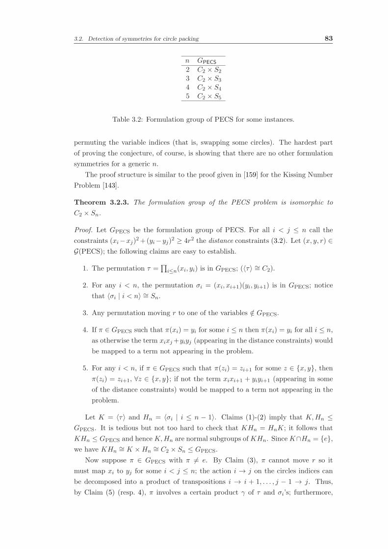
3.2. Detection of symmetries for circle packing 83
n GPECS
2 C2 × S23 C2 × S34 C2 × S45 C2 × S5
Table 3.2: Formulation group of PECS for some instances.
permuting the variable indices (that is, swapping some circles). The hardest part
of proving the conjecture, of course, is showing that there are no other formulation
symmetries for a generic n.
The proof structure is similar to the proof given in [159] for the Kissing Number
Problem [143].
Theorem 3.2.3. The formulation group of the PECS problem is isomorphic to
C2 × Sn.
Proof. Let GPECS be the formulation group of PECS. For all i < j ≤ n call the
constraints (xi−xj)2+(yi−yj)2 ≥ 4r2 the distance constraints (3.2). Let (x, y, r) ∈G(PECS); the following claims are easy to establish.
1. The permutation τ =∏
i≤n(xi, yi) is in GPECS; (〈τ〉 ∼= C2).
2. For any i < n, the permutation σi = (xi, xi+1)(yi, yi+1) is in GPECS; notice
that 〈σi | i < n〉 ∼= Sn.
3. Any permutation moving r to one of the variables /∈ GPECS.
4. If π ∈ GPECS such that π(xi) = yi for some i ≤ n then π(xi) = yi for all i ≤ n,as otherwise the term xixj+yiyj (appearing in the distance constraints) would
be mapped to a term not appearing in the problem.
5. For any i < n, if π ∈ GPECS such that π(zi) = zi+1 for some z ∈ x, y, thenπ(zi) = zi+1, ∀z ∈ x, y; if not the term xixi+1 + yiyi+1 (appearing in some
of the distance constraints) would be mapped to a term not appearing in the
problem.
Let K = 〈τ〉 and Hn = 〈σi | i ≤ n − 1〉. Claims (1)-(2) imply that K,Hn ≤GPECS. It is tedious but not too hard to check that KHn = HnK; it follows that
KHn ≤ GPECS and henceK,Hn are normal subgroups ofKHn. SinceK∩Hn = e,we have KHn
∼= K ×Hn∼= C2 × Sn ≤ GPECS.
Now suppose π ∈ GPECS with π 6= e. By Claim (3), π cannot move r so it
must map xi to yj for some i < j ≤ n; the action i → j on the circles indices can
be decomposed into a product of transpositions i → i + 1, . . . , j − 1 → j. Thus,
by Claim (5) (resp. 4), π involves a certain product γ of τ and σi’s; furthermore,
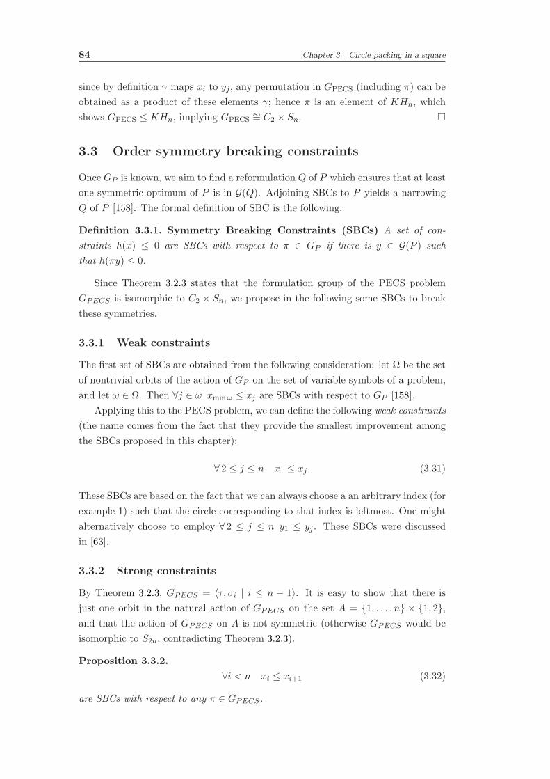
84 Chapter 3. Circle packing in a square
since by definition γ maps xi to yj , any permutation in GPECS (including π) can be
obtained as a product of these elements γ; hence π is an element of KHn, which
shows GPECS ≤ KHn, implying GPECS∼= C2 × Sn.
3.3 Order symmetry breaking constraints
Once GP is known, we aim to find a reformulation Q of P which ensures that at least
one symmetric optimum of P is in G(Q). Adjoining SBCs to P yields a narrowing
Q of P [158]. The formal definition of SBC is the following.
Definition 3.3.1. Symmetry Breaking Constraints (SBCs) A set of con-
straints h(x) ≤ 0 are SBCs with respect to π ∈ GP if there is y ∈ G(P ) such
that h(πy) ≤ 0.
Since Theorem 3.2.3 states that the formulation group of the PECS problem
GPECS is isomorphic to C2 × Sn, we propose in the following some SBCs to break
these symmetries.
3.3.1 Weak constraints
The first set of SBCs are obtained from the following consideration: let Ω be the set
of nontrivial orbits of the action of GP on the set of variable symbols of a problem,
and let ω ∈ Ω. Then ∀j ∈ ω xminω ≤ xj are SBCs with respect to GP [158].
Applying this to the PECS problem, we can define the following weak constraints
(the name comes from the fact that they provide the smallest improvement among
the SBCs proposed in this chapter):
∀ 2 ≤ j ≤ n x1 ≤ xj . (3.31)
These SBCs are based on the fact that we can always choose a an arbitrary index (for
example 1) such that the circle corresponding to that index is leftmost. One might
alternatively choose to employ ∀ 2 ≤ j ≤ n y1 ≤ yj . These SBCs were discussed
in [63].
3.3.2 Strong constraints
By Theorem 3.2.3, GPECS = 〈τ, σi | i ≤ n − 1〉. It is easy to show that there is
just one orbit in the natural action of GPECS on the set A = 1, . . . , n × 1, 2,and that the action of GPECS on A is not symmetric (otherwise GPECS would be
isomorphic to S2n, contradicting Theorem 3.2.3).
Proposition 3.3.2.
∀i < n xi ≤ xi+1 (3.32)
are SBCs with respect to any π ∈ GPECS.

3.3. Order symmetry breaking constraints 85
Proof. Let (x∗, y∗, r∗) ∈ G(PECS); since the σi generate the symmetric group acting
on the n circles, there exists a permutation π ∈ GPECS such that (x∗π(i) | i ≤ n)
are ordered as in (3.32).
We call (3.32) strong constraints, since they are more effective than weak con-
straints for removing symmetries of PECS, as showed by experiments carried out
in [63]. These SBCs are based on the fact that the circles can be ordered on the
horizontal axis. Again, one can alternatively employ ∀i < n yi ≤ yi+1.
It is interesting to see experimentally the effect of these SBCs on the solution
process of the local solver employed by the sBB algorithm. As mentioned in Section
3.2, we observe that good feasible solutions were found earlier in the search with
SBCs rather than without.
All our experiments in this chapter are conducted using the Couenne sBB solver
(trunk version dated November 2010) with the default configuration, which employs
the IpOpt [244] subsolver as the local NLP solver used to find incumbents in Step
4 of the sBB algorithm given in Section 1.2.2.5. IpOpt actually solves the following
PECS reformulation:
−min − r (3.33)
s.t. ∀i < j ≤ n (xi − xj)2 + (yi − yj)2 − 4r2 − si,j = 0 (3.34)
∀i ≤ n xi − r − Lxi = 0 (3.35)
∀i ≤ n yi − r − Lyi = 0 (3.36)
∀i ≤ n xi + r − 1 + Uxi = 0 (3.37)
∀i ≤ n yi + r − 1 + Uyi = 0 (3.38)
∀i < j ≤ n Lxi ∈ R
+0 (3.39)
∀i < j ≤ n Lyi ∈ R
+0 (3.40)
∀i < j ≤ n Uxi ∈ R
+0 (3.41)
∀i < j ≤ n Uyi ∈ R
+0 (3.42)
∀i < j ≤ n si,j ∈ R+0 (3.43)
∀i ≤ n xi ∈ R+0 (3.44)
∀i ≤ n yi ∈ R+0 (3.45)
r ∈ R+0 , (3.46)
obtained by introducing slack variables for each inequality. The natural starting
point for solving (3.33)-(3.46) in Step 4 is the solution of the relaxation in Step 2,
which is ∀i ≤ n xi = yi = r = 12 at the root node by Proposition 3.2.1. Since
this is infeasible with respect to (3.34), IpOpt starts with a feasibility restoration
phase, converging to the starting point ∀i ≤ n xi = yi = 12 , r = 0. It is long
and tedious, but easy, to check that Linear Independence Constraints Qualification
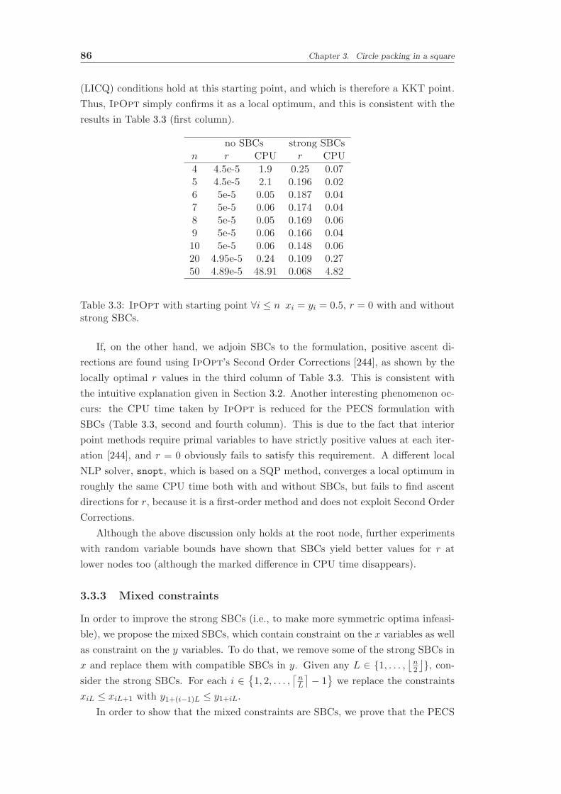
86 Chapter 3. Circle packing in a square
(LICQ) conditions hold at this starting point, and which is therefore a KKT point.
Thus, IpOpt simply confirms it as a local optimum, and this is consistent with the
results in Table 3.3 (first column).
no SBCs strong SBCsn r CPU r CPU
4 4.5e-5 1.9 0.25 0.075 4.5e-5 2.1 0.196 0.026 5e-5 0.05 0.187 0.047 5e-5 0.06 0.174 0.048 5e-5 0.05 0.169 0.069 5e-5 0.06 0.166 0.0410 5e-5 0.06 0.148 0.0620 4.95e-5 0.24 0.109 0.2750 4.89e-5 48.91 0.068 4.82
Table 3.3: IpOpt with starting point ∀i ≤ n xi = yi = 0.5, r = 0 with and withoutstrong SBCs.
If, on the other hand, we adjoin SBCs to the formulation, positive ascent di-
rections are found using IpOpt’s Second Order Corrections [244], as shown by the
locally optimal r values in the third column of Table 3.3. This is consistent with
the intuitive explanation given in Section 3.2. Another interesting phenomenon oc-
curs: the CPU time taken by IpOpt is reduced for the PECS formulation with
SBCs (Table 3.3, second and fourth column). This is due to the fact that interior
point methods require primal variables to have strictly positive values at each iter-
ation [244], and r = 0 obviously fails to satisfy this requirement. A different local
NLP solver, snopt, which is based on a SQP method, converges a local optimum in
roughly the same CPU time both with and without SBCs, but fails to find ascent
directions for r, because it is a first-order method and does not exploit Second Order
Corrections.
Although the above discussion only holds at the root node, further experiments
with random variable bounds have shown that SBCs yield better values for r at
lower nodes too (although the marked difference in CPU time disappears).
3.3.3 Mixed constraints
In order to improve the strong SBCs (i.e., to make more symmetric optima infeasi-
ble), we propose the mixed SBCs, which contain constraint on the x variables as well
as constraint on the y variables. To do that, we remove some of the strong SBCs in
x and replace them with compatible SBCs in y. Given any L ∈ 1, . . . ,⌊
n2
⌋
, con-sider the strong SBCs. For each i ∈
1, 2, . . . ,⌈
nL
⌉
− 1
we replace the constraints
xiL ≤ xiL+1 with y1+(i−1)L ≤ y1+iL.
In order to show that the mixed constraints are SBCs, we prove that the PECS

3.3. Order symmetry breaking constraints 87
formulation with the mixed constraints adjoined is a narrowing of the PECS formu-
lation. We define the following index sets:
• N = 1, . . . , n
• N ′ = 1, . . . , n− 1
• N ′′ = 1, L+ 1, 2L+ 1, . . . , (⌈n/L⌉ − 2)L+ 1,
the following sets of constraints (intended as list of symbolic expressions representing
the constraints, rather than sets of real vectors feasible with the constraints):
• S = xi ≤ xi+1 | i ∈ N ′
• ∀i ∈ N ′′ Ai = xh ≤ xh+1 | h ∈ N ′r i+ L− 1
• ∀i ∈ N ′′ Ci = yi ≤ yi+L,
and the following formulations:
• PECS′ ≡ PECS ∪S (i.e., the PECS formulation with strong constraints)
• ∀i ∈ N ′′ PECSi ≡ PECS ∪Ai ∪ Ci,
• PECS′′ ≡ PECS ∪⋃i∈N ′′(Ai ∪ Ci).
Proposition 3.3.3. For all i ∈ N ′′, PECSi is a narrowing of PECS.
Proof. Let i ∈ N ′′ and (x∗, y∗, r∗) ∈ G(PECS). For a permutation π ∈ Sn we
assume π(x∗, y∗, r∗) = (πx∗, πy∗, πr∗) where π acts on a vector in Rn by permuting
the indices of its components; notice that since π is simply a reindexing of the circles,
π(x∗, y∗, r∗) ∈ G(PECS). Furthermore, since PECS′ is known to be a narrowing of
PECS, we can assume WLOG that (x∗, y∗, r∗) satisfies S . If y∗i ≤ y∗i+L the result
holds, otherwise assume y∗i > y∗i+L. Consider the permutation σi =∏L−1
ℓ=0 (i +
ℓ, i + L + ℓ) in Sn; σi(x∗, y∗, r∗) has the following properties: (a) by the action
of the 2-cycle (i, i + L) (appearing in σi when ℓ = 0) we have y∗i < y∗i+L; (b)
∀ℓ ∈ 0, . . . , L − 2 we have σix∗i+ℓ = x∗i+L+ℓ ≤ x∗i+L+ℓ+1 = σix
∗i+ℓ+1 and
σix∗i+L+ℓ = x∗i+ℓ ≤ x∗i+ℓ+1 = σix
∗i+L+ℓ+1; (c) ∀h ∈ N ′ such that h 6∈ Hi =
i, . . . , i + 2L − 1 we have σix∗h = x∗h ≤ x∗h+1 = σix
∗h+1 because σi fixes all
h 6∈ Hi. Thus σi(x∗, y∗, r∗) ∈ G(PECS) and satisfies the constraints of PECSi.
Lemma 3.3.4. Let t = ⌈n/L⌉ − 1 and Σ = σi | i ∈ N ′′. Then 〈Σ〉 ∼= St.
Proof. Notice N ′′ = (j− 1)L+1 | 1 ≤ j ≤ t, and define a map ϕ((j− 1)/L+1) =
j, under which ϕ(Σ) = (1, 2), (2, 3), . . . , (t − 1, t). This map induces a group
homomorphism ϕ : 〈Σ〉 → St given by ϕ(σi) = (ϕ(i), ϕ(i)+1), which can be verified
to be injective and surjective.

88 Chapter 3. Circle packing in a square
Similarly, for all h < k ∈ N ′′ we have 〈Σhk〉 = 〈σi | h ≤ i < k〉 ∼= Sym(Ihk),
the symmetric group on the set Ihk = ϕ(h), . . . , ϕ(k). Thus, for all h, k ∈ N ′′,
the permutation τhk =∏L−1
ℓ=0 (h + ℓ, k + ℓ) can be obtained as a certain product of
the σi’s for i ∈ ϕ−1(Ihk). More precisely, we have τhk = (ϕ(k) − 1, ϕ(k))(ϕ(k) −2, ϕ(k)− 1) · · · (ϕ(h), ϕ(h) + 1)(ϕ(h) + 1, ϕ(h) + 2) · · · (ϕ(k)− 1, ϕ(k)).
Theorem 3.3.5. PECS ′′ is a narrowing of PECS.
Proof. Let (x∗, y∗, r∗) ∈ G(PECS), and consider the set V of all constraints Ci ≡yi ≤ yi+L violated by (x∗, y∗, r∗). Let ψ be the (invertible) map given by ψ(Ci) =
(ϕ(i), ϕ(i) + 1); then ψ(V ) is a set of transpositions that can be partitioned into
maximal non-disjoint subsets Shk = (ϕ(h), ϕ(h) + 1), . . . , (ϕ(k) − 1, ϕ(k)); let T
be the set of pairs (h, k) for which Shk is in the partition of ψ(V ). It is easy to verify
that if πhk =∏
ℓ∈Ihk
h+ℓL<k−ℓL
τh+ℓL,k−ℓL then πhky∗ satisfies the constraints in ψ−1(Shk).
Furthermore, by maximality of the Shk, the permutations πhk are disjoint. Now, if
π =∏
(h,k)∈Tπhk, π(x
∗, y∗, r∗) is such that πy∗ satisfies all constraints in V and
πx∗ satisfies all constraints in⋃
i∈N ′′ Ai by Proposition 3.3.3. Thus π(x∗, y∗, r∗) ∈G(PECS′′).
3.3.4 Numerical results
It has been shown in [59] that mixed constraints are more effective to remove sym-
metries than strong constraints, so we consider now the PECS model with mixed
SBCs.
First, from previous section it appears that mixed SBCs rely on an arbitrary
choice for the integer L. Figure 3.4 shows the number of sBB tree nodes in function
of L for the instances from n = 4 to n = 9. These experiments indicate that
L = 2 is the best choice (Note that the choice L = 1 is not considered since it
corresponds to removing all the strong constraints on the x variables and to adjoin
the corresponding constraints on the y variables).
In order to test the mixed constraints, we first provide empirical evidence that
the proposed SBCs tighten the upper bound in Step 2 of Section 1.2.2.5 by solving
a set of small PECS instances to global optimality using the Couenne solver on a
2.4 GHz Intel Xeon CPU with 24 GB RAM running Linux. Table 3.4 reports the
instance (n), the globally maximum possible radius r∗ allowing a packing of n circles
in the unit square, the number of sBB nodes, and the seconds of user CPU time
taken by Couenne running to termination on the original formulation and on the
narrowing.
A second set of tests concerns the performance of Couenne on the mixed SBC
based narrowing with early termination based on two hours of user CPU time. In
Table 3.5 we report the number of circles, the best known solution r (taken from
http://www.packomania.com; a proof of optimality is only given for instances where

3.3. Order symmetry breaking constraints 89
2 3−1
−0.8
−0.6
−0.4
−0.2
0
0.2
0.4
0.6
0.8
1
L
Nod
es
4 circles
2 3 40
0.2
0.4
0.6
0.8
1
1.2
1.4
1.6
1.8
2
L
Tre
e no
des
5 circles
2 3 4 50
10
20
30
40
50
60
70
80
90
100
L
Tre
e no
des
6 circles
2 3 4 5 60
500
1000
1500
2000
2500
3000
3500
4000
L
Tre
e no
des
7 circles
2 3 4 5 6 70
1
2
3
4
5
6
7x 10
4
L
Tre
e no
des
8 circles
2 3 4 5 6 7 80
0.2
0.4
0.6
0.8
1
1.2
1.4
1.6
1.8
2x 10
6
L
Tre
e no
des
9 circles
Figure 3.4: sBB tree nodes in function of L.
Original formulation Mixed SBC Narrowingn r∗ sBB nodes CPU time sBB nodes CPU time
2 0.292893 2 0.04 0 0.023 0.254333 2 0.15 0 0.084 0.25 282 1.85 0 0.085 0.207113 68710 69.24 541 2.026 0.187707 3087798 6176.05 42850 90.84
Table 3.4: sBB running to termination on small PECS instances.
n ≤ 30 and n = 36), the solution found at the root node rr, the largest radius r
found by our method within the time limit, the tightest upper bound r (which gives
an idea of the optimality gap), the time t(r) at which the solution r was found, and
the number of nodes explored within the time limit.
The mixed SBCs both tighten the problem relaxation and, rather unexpectedly,

90 Chapter 3. Circle packing in a square
n r rr r r t(r) sBB nodes
20 0.111382 0.111382 0.111382 0.322063 16.45 44182825 0.1 0.096852 0.1 0.250133 553.68 12563230 0.091671 0.091671 0.091671 0.316273 86.24 9023035 0.084290 0.082786 0.083766 0.351545 1495.31 4616240 0.079186 0.078913 0.078913 0.2501 19.68 1711645 0.074727 0.07444 0.07444 0.353325 357.90 1291550 0.071377 0.070539 0.070539 0.250121 5429.88 2
Table 3.5: sBB running on large PECS instances.
ease the work of the local solver deployed at each node. An interesting fact is that
the formulation with mixed SBCs leads to solutions very close to the best known
already at the root node of the sBB tree, as shown in Table 3.5.
3.4 Other constraints
In this section we present other constraints which are useful to tighten the PECS
formulation. We consider as starting model the PECS formulation (3.1)-(3.5) with
the strong SBCs (3.32) adjoined. We use the strong constraints because they are
necessary to derive some of the inequalities presented in the following.
3.4.1 Fixing points symmetry breaking constraints
In [173], the authors present the following theorem for PPS (a proof can be found
in [172,209]):
Theorem 3.4.1. There always exists an optimal solution of the PPS problem such
that at each vertex v of the unit square, incident to the sides e1 and e2, one and only
one of the following statements holds:
• a point of the optimal solution is in the vertex v;
• two points of the optimal solution belong to the sides e1 and e2 and have dis-
tance equal to the optimal one.
Starting from this theorem we can prove the following:
Theorem 3.4.2. Consider the PPS problem with n ≥ 4. There is always an optimal
solution where at least two points are on the left side of the square, and at least two
points are on the right side of the square.
Proof. Consider the left side of the square, and call v1 the bottom-left vertex, while
v2 is the top-left one; by Theorem 3.4.1, we can have four different situations:
(a) we have a point (p1) in v1 and one (p2) in v2;

3.4. Other constraints 91
(b) we have a point (p1) in v1, and we have 2 other points: one on the left side
of the square (p2), one on the top side (p3) whose distance is the optimal one
m∗;
(c) we have a point (p2) in v2, and we have 2 other points: one on the left side of
the square (p1), one on the bottom side (p4) whose distance is the optimal one
m∗;
(d) we have one point on the left side of the square (p2) and one on the top side (p3)
whose distance is the optimal one m∗; furthermore, we have another point on
the left side (p1) and one on the bottom side (p4) whose distance is the optimal
one m∗.
In all these cases, that are presented in Figure 3.5, we have at least two points on
the left side of the square.
(a) (b) (c) (d)
Figure 3.5: Possible configurations of points in the optimal solution of PPS accordingto Theorem 3.4.1.
All that remains to be shown is that in cases 3.5(b), 3.5(c), 3.5(d), the points p1
and p2 cannot coincide. For cases (b) and (c) if p1 = p2 then m∗ > 1. This is not
possible since the optimal distance when n = 4 is equal to 1, and for larger instances
the distance decreases. Consider now the case (d). Suppose that p1 = p2, that v1
has coordinates (0,0) and call ya the distance between v1 and p1 (hence the distance
between p1 and v2 is equal to 1 − ya). The distance m∗ is equal to the distance
between p1 and p4, and the coordinate x of p4 is in (0, 1). Similarly, m∗ is equal to
the distance between p1 and p3, and the coordinate x of p3 is in (0, 1). Hence the
following inequalities hold:
1− ya < m∗ <√
1 + (1− ya)2
ya < m∗ <√
ya2 + 1,
where ya ∈ (0, 1). Comparing these inequalities, it turns out that in order to have
a valid value of m∗ the intervals[
1− ya,√
1 + (1− ya)2]
and[
ya,√
ya2 + 1]
must
have a nonempty intersection. To ease the following steps we can apply the square

92 Chapter 3. Circle packing in a square
operator to the previous inequalities (since all the terms are positive), thus obtaining:
(1− ya)2 < m∗2 < 1 + (1− ya)2
ya2 < m∗2 < ya
2 + 1.
In order to check that the intersection is nonempty, one should derive an order
relationship between the left and right-hand sides of these inequalities. Since ya ∈(0, 1), we have actually 3 cases to consider:
• ya ∈(
0, 12)
. In this case the order relationship is the following: ya2 < (1 −
ya)2 < ya
2 + 1 < 1 + (1 − ya)2. Thus, m∗2 must be between (1 − ya)2 and
ya2 + 1. In other words, we have that 1− ya < m∗ <
√
ya2 + 1, ya ∈(
0, 12)
;
• ya ∈(
12 , 1)
. In this case the order relationship is the following: (1 − ya)2 <ya
2 < 1+(1−ya)2 < ya2+1. Thus, m∗2 must be between ya
2 and 1+(1−ya)2.In other words, we have that ya < m∗ <
√
1 + (1− ya)2, ya ∈(
12 , 1)
;
• ya = 12 . In this case we have (1−ya)2 = ya
2 = 14 and 1+(1−ya)2 = ya
2+1 = 54 .
Hence, 12 < m∗ <
√52
In all these cases, the resulting inequality is the following:
1
2< m∗ <
√5
2. (3.47)
This means that we can have p1 = p2 only if the optimal distance satisfies the
inequality (3.47). We are considering the instances having n ≥ 4. When n = 4, the
optimal distance is 1, that is less than√52 . The optimal distance when n = 9 is equal
to 12 , and for larger instances the optimal distance decreases. This means that the
only possibilities for having p1 = p2 are the instances where 4 ≤ n ≤ 8. However, in
these cases the optimal solutions are known, and there are always at least 2 points on
a side of the square, as can be checked in [237] or in http://www.packomania.com.
Hence, it is not possible that p1 and p2 coincide.
A similar idea can be used to prove the same for the right side of the square.
Moreover, it is true even if we consider the other pair of opposite sides (that is
top/bottom) in place of the left/right ones.
This result can be extended to the PECS problem in order to obtain some con-
straints, as proved by the following corollary.
Corollary 3.4.3. Consider the PECS problem with n ≥ 4, where the strong SBCs
(3.32) hold. The following constraints are valid:
∀i ∈ 1, 2 xi = r (3.48)
∀i ∈ n− 1, n xi = 1− r. (3.49)

3.4. Other constraints 93
Proof. Using the result of Theorem 3.4.2 and looking at Figure 3.1 it is obvious that
for PECS problem there is always an optimal solution where at least two points are
at distance r from the left side of the square, and at least two points are at distance
r from the right side of the square. Thus, we can fix 2 points at distance r to the
left side of the square, and other 2 points at distance r from the right side of the
square. Since we want to respect also the strong SBCs (3.32), we can express that
by means of the constraints (3.48) and (3.49).
3.4.2 Bounds symmetry breaking constraints
As remarked in [11], the following statements hold WLOG:1
• at least nx = ⌈n2 ⌉ points are on the left half of the square (x bound constraints);
• among the previous nx points, at least ny = ⌈nx
2 ⌉ are on the bottom half (y
bound constraints).
Unfortunately, this is not true if we have also the strong SBCs: for example, the
optimal solution of the PECS problem when n = 8 does not respect all these con-
straints together. In fact, as can be seen in Figure 3.6, if the solution respects both
the strong SBCs and the x bound constraints we cannot have the circles 1 and 2 in
the bottom half of the square (that is y1 ≤ 12 and y2 ≤ 1
2 , since ny = 2), so the y
bound constraints do not hold.
Figure 3.6: Optimal solution of PECS for n = 8 (this figure is taken fromhttp://www.packomania.com).
We can conclude that the x bound constraints can be adjoined to the PECS
model with strong SBCs, but not together with the y bound constraints. Actually,
1The symmetric condition consisting of placing the first nx points on the right half of the squareand then the first ny on the top half, considered in [11], is equivalent to the one presented here.This is because in that paper the strong constraints were considered with opposite sign, that isxi ≥ xi+1 instead of xi ≤ xi+1 as defined in (3.32).

94 Chapter 3. Circle packing in a square
as claimed in [11], it is possible to have together the strong SBCs, the x bound
constraints, and the y bound constraints if we drop the strong SBC xny ≤ xny+1.
However, we need to preserve all the strong SBCs to derive the“triangular inequality
constraints” presented in Section 3.4.3.
Hence, we show how to formulate in another way the y bound constraints, in
order to add them to the model, and how to add the x bound constraints using a
single inequality.
The latter can be done this way: since the strong SBCs hold, it is sufficient to
add the following inequality:
xnx ≤1
2. (3.50)
Thus, the inequalities ∀i ≤ nx xi ≤ 12 are automatically satisfied.
The former problem is basically the following: among the nx points that are on
the left half of the square, at least ny are on the bottom half, but we cannot know
which points are on the bottom half; nevertheless, we can obtain an inequality on
the sum of the y components of the first nx points.
More precisely, ny points have the coordinates y which are smaller than or equal
to 12 . For the others nx − ny the y coordinates are smaller than or equal to 1 − r.
Hence, we can write the following inequality:
nx∑
i=1
yi ≤ny2
+ (nx − ny)(1− r). (3.51)
Using the same idea, we can obtain something similar for the sum of the x
components of all the points.
Basically, nx points have the coordinates x that are smaller than or equal to 12 ;
among them, two have coordinates fixed to r, as shown by (3.48). For the others
n − nx the x coordinates are smaller than or equal to 1 − r. So, we can write this
inequality:n∑
i=1
xi ≤1
2(nx − 2) + 2r + (n− nx)(1− r). (3.52)
It is interesting to notice that the constraint (3.52) might seem redundant if we
have the constraints (3.3), (3.32), (3.48), and (3.50). Actually, some tests show that
this inequality helps to obtain better upper bounds, above all with big instances of
PECS. The reason for this behavior could be that Couenne uses this constraint to
derive some cuts, which are automatically adjoined to the MP model.
3.4.3 Triangular inequality constraints
From the triangular inequality, we can write:
∀i < j ≤ n |xj − xi|+ |yj − yi| ≥ dij ≥ 2r, (3.53)

3.4. Other constraints 95
where dij represents the distance between the centers of the circles i and j.
The strong SBCs imply that ∀i < j ≤ n xj − xi ≥ 0. Hence, we can remove the
absolute value on the x variables from (3.53) obtaining:
∀i < j ≤ n xj − xi + |yj − yi| ≥ 2r. (3.54)
Our aim is to remove the absolute value from the y variables, since it is a source
of nonlinearity and makes the inequality difficult to solve. In order to get the final
set of constraints, we should prove the following proposition:
Proposition 3.4.4. Given the constraints (3.2)-(3.5) of the PECS formulation and
the strong SBCs, the following inequalities hold:
∀i < j ≤ n yj + yi ≥ |yj − yi|+ 2r.
Proof. We can suppose WLOG that yj ≥ yi (if not the proof produces a similar
result). Hence ∀i < j ≤ n yj + yi ≥ yj − yi + 2r. This is equivalent to ∀i < j ≤n yi ≥ r, that is obviously true, since these inequalities are implied by (3.4).
At this point, we can remove the absolute value on the y variables from (3.54)
by replacing |yj − yi| with yj + yi − 2r:
∀i < j ≤ n xj − xi + yj + yi − 2r ≥ xj − xi + |yj − yi| ≥ 2r.
Finally we obtain the constraints:
∀i < j ≤ n xj − xi + yj + yi ≥ 4r. (3.55)
3.4.4 Numerical results
In this section we compare two formulations of PECS for the instances where 4 ≤n ≤ 20: the original formulation (3.2)-(3.5) with the strong SBCs (PECS + strong),
and the same formulation with all the new constraints proposed in Section 3.4, i.e.,
(3.48)-(3.52) and (3.55) (PECS + all). Our comparative results, shown in Table
3.6, have been obtained on a 2.4 GHz Intel Xeon CPU with 24 GB RAM running
Linux and the solver Couenne; the table displays the following statistics for the two
formulations: objective function value f∗ of the incumbent, gap still open (we use
the CPLEX definition [135]:(
100·|f∗−fUB ||f∗+10−10|
)
%, where fUB is the best upper bound
found in the case of maximization problems), number of BB nodes closed, number of
BB nodes still on the tree, and the CPU time (in seconds) taken, with a time limit
of 2h. Moreover, we show also the optimal solutions r∗ for the instances, which can
be found in [237] or in http://www.packomania.com.
The new constraints proposed in this section increase significantly the perfor-
mance of Couenne with respect to the PECS formulation with strong SBCs, as

96 Chapter 3. Circle packing in a square
PECS + strong PECS + all
n r∗ f∗ gapn. closedn. on tree CPU time f∗ gap
n. closedn. on tree CPU time
4 0.25 0.25 0%
00 0.12 0.25 0%
00 0.13
5 0.207107 0.207107 0%
20 0.44 0.207107 0%
20 0.19
6 0.187681 0.187703 0%
84560 17.90 0.187713 0%
1100 7.25
7 0.174458 0.174458 0%
2451020 728.69 0.174458 0%
5640 17.11
8 0.170541 0.170541 17.71%1853359117869 7200 0.170541 0%
78220 65.78
9 0.166667 0.166667 30.55%1365445279773 7200 0.166667 0%
660700 525.75
10 0.148204 0.148201 65.10%1230472334114 7200 0.148204 32.22%
611560201488 7200
11 0.142399 0.142399 75.62%1068775290037 7200 0.142339 39.61%
498050179367 7200
12 0.139959 0.139959 78.64%899535273315 7200 0.139959 59%
365384136656 7200
13 0.133994 0.133993 110.67%816573232735 7200 0.133993 53.57%
337112133403 7200
14 0.129332 0.129332 119.10%615348182939 7200 0.129332 74.04%
25040697740 7200
15 0.127167 0.126478 124.75%853025245904 7200 0.127167 77.19%
20485381901 7200
16 0.125 0.125 100.38%382247121598 7200 0.125 77.40%
17376770580 7200
17 0.117197 0.116293 115.19%27509498707 7200 0.117111 91.16%
14800461668 7200
18 0.115521 0.113218 175.46%433224140861 7200 0.115521 101.74%
12964153367 7200
19 0.112265 0.11174 179.20%454058158505 7200 0.111911 104.83%
11148644392 7200
20 0.111382 0.111382 210.63%342260116599 7200 0.111382 108.65%
9027435542 7200
Table 3.6: Results obtained by running Couenne on some PECS instances.
shown in Table 3.6. As a matter of fact, the time to obtain the optimal solution is
lower, and when the time limit is reached for both formulations, the gap is smaller.
This means that the formulation “PECS + all” leads to a lower value of the upper
bound for r (since the value of the best solution found by “PECS + all” is always
greater than or equal to that of the “PECS + strong” formulation).
Looking at the number of nodes on the sBB tree, we can see that the trees
associated to the “PECS + all” formulation are smaller than the trees obtained with
“PECS + strong”, as expected. Furthermore, in four cases the incumbent found
with the “PECS + all” formulation is better than the one found with the “PECS
+ strong” formulation (in two cases, n = 15 and n = 18, the value is equal to the
optimum). Hence, even if we test these formulations on a small number of instances,
it is quite evident that “PECS + all” outperforms “PECS + strong”.
Looking at the n = 6 case in the table, we see that the incumbent values found are
higher than the optima, but this is due to the numerical approximation of Couenne.
3.5 A conjecture about the reduction of the search space
In this section we present a conjecture about the tightening of some of the bound of
the variables of PPS. The extension to the PECS problem is presented at the end.
When we try to solve the PPS problem by means of sBB, usually the root node

3.5. A conjecture about the reduction of the search space 97
corresponds to a linear relaxation of the problem, whose optimal solution represents
an upper bound for the original problem. For the PPS formulation (3.6)-(3.10) the
relaxation is the following (as explained in [173,209]):
max α (3.56)
s.t. ∀i < j ≤ n − l(i, j) ≥ α (3.57)
∀i ≤ n xi ∈ [0, 1] (3.58)
∀i ≤ n yi ∈ [0, 1] (3.59)
α ∈ R+0 , (3.60)
where l(i, j) = −(Lxi− Uxj
+ Uxi− Lxj
)(xi − xj) − (Lyi − Uyj + Uyi − Lyj )(yi −yj)+ (Lxi
−Uxj)(Uxi
−Lxj)+ (Lyi −Uyj )(Uyi −Lyj ) represents the convex envelope
of the nonlinear part of constraint (3.2), while Lxi, Lyi , Uxi
, and Uyi represent the
lower and upper bounds on the x and y variables (in this case, the lower bounds are
equal to 0 and the upper bounds are equal to 1 for all the variables).
Proposition 3.5.1. The optimal solution of the problem (3.56)-(3.60) is α∗ = 2.
Proof. It is easy to see that when all the lower bounds have the same value L, and
the upper bounds have the same value U , then −l(i, j) = 2(U − L)2. Considering
the problem of maximizing α, with the constraints ∀i < j ≤ n α ≤ 2(U − L)2, theobjective function value of the optimal solution is α∗ = 2(U −L)2. Since L = 0 and
U = 1, then α∗ = 2.
The bound provided by the previous relaxation is roughly loose: since α is the
square of the minimum distance between the points, the upper bound on the distance
is√2, that is the cost of the optimal solution obtained when there are only 2 points
in the square, placed in two opposite vertices. Furthermore, this bound does not
depend on the number of points n, nor on the value of the variables x and y: due
to the fact that all the lower and upper bounds have the same value, in the linear
relaxation l(i, j) all the coefficients of the terms containing x and y become 0.
In order to improve the value of α∗, we should change the value of lower and
upper bounds for some variables; thus, the corresponding terms containing x and
y in the linear relaxation do not disappear. The following conjecture refers to that
idea.
Conjecture 3.5.2. Consider an instance of PPS with n points. Divide the unit
square in k2 equal subsquares, with k = argmin∣
∣
n2 − s2
∣
∣, s ∈⌈√
n2
⌉
,⌊√
n2
⌋
. There
is at least one point of the optimal solution in each subsquare.
The meaning of this conjecture is that we can change the value of the bounds
for k2 points. For example, consider the case with n = 9: here, k = 2, so there are 4

98 Chapter 3. Circle packing in a square
Original formulation bound constraints formulationn m∗ LB UB LB UB
9 0.5 0.000098 1.414213 0.300463 0.70710710 0.421279 0.000098 1.414213 0.396156 0.70710711 0.398207 0.000099 1.414213 0.000099 0.70710712 0.388730 0.000099 1.414213 0.360065 0.70710713 0.366096 0.000098 1.414213 0.339654 0.50294814 0.348915 0.000098 1.414213 0.340830 0.50287415 0.341081 0.000098 1.414213 0.334524 0.50279316 0.333333 0 1.414213 0.290033 0.50279317 0.306153 0 1.414213 0.000099 0.50279318 0.300462 0 1.414213 0.252819 0.50279319 0.289541 0.000047 1.414213 0.252337 0.50279320 0.286611 0 1.414213 0.276468 0.502793
Table 3.7: Results obtained at the root node of the sBB tree by Couenne for someinstances of PPS with and without range tightening of the variables.
subsquares. According to the conjecture, we can place one point in each subsquare;
for instance, if we put the point i is in the bottom left subsquare, we can modify the
bounds provided by (3.8) obtaining xi ≤ 0.5 and yi ≤ 0.5.
In order to change other bounds, we can use the x bound constraints and the
y bound constraints presented in Section 3.4.2. After dividing the square in k2
subsquares, we have placed in the left half of the square η < nx points, so for other
nx − η points we can change the upper bounds on the coordinates x from 1 to 0.5,
according to the x bound constraints. A similar idea can be used for the y bound
constraints.
Table 3.7 presents the values of the upper and lower bounds for some instances
of the PPS problem obtained at the root node of the sBB of Couenne, with and
without the constraints derived from Conjecture 3.5.2. The value of the upper bound
is obtained by solving a linear relaxation of the problem, whereas the lower bound
is the best solution found so far. The values of the optimal distance d∗ =√α∗ are
also reported (they can be found in http://www.packomania.com and in [237]).
The results presented in Table 3.7 show that using the range tightening con-
straints the upper bounds are better, as well as the lower bounds which in some
cases provide solutions not far from the optimal ones. Moreover, we can see an
improvement of the upper bounds from the instance n = 12 (where k = 3) to the
instance n = 13 (where k = 4). The fact that without these constraints the quality
of the solution at the root node is poor can be seen as another side effect of symme-
tries, since having the upper (lower) bounds equal for all the variables yields a bad
linear relaxation of the problem, as show by Proposition 3.5.1.
In order to extend this result to the PECS problem, one should divide the square
[r, 1−r]2 in k2 subsquares, instead of dividing the [0, 1]2 square as done for PPS (it is
more clear if looking at Figure 3.1). For example, if k = 3 we obtain 9 subsquares of

3.6. Conclusions 99
side 1−2r3 . Then, the center of the circle i which is inside the left bottom subsquare
has xi ∈[
r, r + 1−2r3
]
and yi ∈[
r, r + 1−2r3
]
.
3.6 Conclusions
In this chapter we presented the problem of packing equal circles in a square as ex-
ample of optimization problem involving a high degree of symmetries. The presence
of symmetric optima is a problem for sBB algorithms, since the BB tree becomes
large and the time to reach the leaves, i.e., the optimal solutions, increases. In order
to make some of the symmetric optima infeasible we proposed some reformulations
of the original model. In the first part of the chapter we presented different formula-
tions for the problem of packing equal circles in a square (i.e., PECS and PPS), and
we show some numerical results which support our decision to employ the PECS
formulation. Then, we introduced three classes of SBCs, called weak, strong, and
mixed, which yield narrowing reformulations. The mixed SBCs based formulation
was the most effective to remove symmetries, and it provides good quality solu-
tion already at the root node of the BB tree. In the second part of the chapter
we proposed some other inequalities to tighten the formulation. Starting from the
PECS formulation with strong SBCs, we derived a new formulation which can be
solved faster. We used strong SBCs and not mixed SBCs because some of these new
inequalities needed the strong SBCs to be valid.
In the last part of the chapter we presented a conjecture about the reduction
of the variables range. We used the PPS formulation in this case, since it is easier
to describe the conjecture, but we extended also the result for PECS. Basically, we
stated that the unit square can be divided in a number of subsquares that is close
to half of the number of points n of the PPS instance, and that in the optimal
solution each subsquare contains at least a point. Looking at the optimal and best
known solutions this conjecture seems always to be valid (furthermore, it seems the
number of subsquares can also be increased). The effect of this conjecture is that
the new tight ranges of the variables associated to the points which belong to these
subsquares yield to both a better upper bound and a better incumbent already at
the root node of the sBB tree. The effect of having bad quality solutions at the root
node was also observed when introducing SBCs, and the results were better with
the SBCs-based formulations.
Even if we did not improve the best known solutions (in terms of value of the
objective function), this chapter in interesting to show the effect of symmetries
in MP and some techniques to remove them. However, the best results found in
the literature for PECS are obtained mostly by heuristics and specifically designed
algorithms. Albeit we were able to remove all the symmetries, the problem would
still be hard because it is nonlinear and nonconvex, and sBB based algorithms would
not be able to solve large instances.

100 Chapter 3. Circle packing in a square

Part III
An application of relaxations


103
This part of the thesis concerns the comparison of two methods, called respectively
primal and dual, to represent the convex relaxations for multilinear terms. More
precisely, the primal relaxation consists of replacing each multilinear term with a new
variable, and a set of constraints to be adjoined to the model. The dual relaxation
is obtained using the dual representation of the convex (lower)/concave (upper)
envelopes associated to each multilinear term, i.e., the convex combination of their
extreme points using dual variables λ. The theory underlying these relaxations is
well-known, hence the contribution of this chapter is not theoretical. Rather, we
present a computational analysis which shows that the dual approach leads to a
formulation that is easier to write, is more stable, and that can be solved faster
with respect to the model obtained using the primal approach, when the number of
multilinear terms increases. Moreover, the primal relaxation can be written in an
optimal way (in some sense) only for bilinear and trilinear problems, and partly for
quadrilinear problems, whereas the dual approach can be used for any multilinear
term. This work has been presented in [62].

104

Chapter 4Primal and dual convex relaxations for
multilinear terms
Several problems in the literature are described by means of MP models where
products of k variables x1 · · ·xk can appear in the constraints and in the objective
function. The corresponding term is called bilinear if k = 2, trilinear if k = 3,
quadrilinear if k = 4, and so on. In general, they are called multilinear terms.
Among the most well-known applications involving multilinear terms, there are
pooling and blending problems [4,14,67,96,124,191], where bilinear products occur
whenever x1 indicates a percentage and x2 an oil flow in a pipe. The Hartree-Fock
problem [163] minimizes a quartic energy expression (involving quadrilinear terms)
subject to some orthogonality constraints (involving bilinear terms). The molecular
distance geometry problem [164] involves bilinear or quadrilinear terms depending on
which formulation is used. General multilinear terms involving continuous variables
occur in multilinear least-squares problems [202]. In general, such products occur
over bounded variables: most applications require the variables x = (x1, . . . , xk)
to be bounded to the hyperrectangle [xL, xU ], where xL = (xL1 , . . . , xLk ) and xU =
(xU1 , . . . , xUk ). We remark, however, that there exists an application from code de-
bugging [109, 165] exhibiting bilinear terms x1x2 where x1 ∈ 0, 1 and x2 must be
unbounded for the model to be correct (such variables are used to ensure that loops
terminate whenever no upper bound is explicitly known for the loop counter).
Since the models having multilinear terms are nonconvex and nonlinear, one
must employ sBB algorithms in order to obtain a guaranteed solution. sBB methods
employ a convex relaxation of the problem at each search node. Such relaxations can
be obtained in two ways: the traditional method consists of representing the convex
hull (defined by convex and concave envelopes) by means of a set of inequalities to
adjoin to the original model. One can alternatively use the dual representation of
these envelopes, i.e., the convex combinations of the extreme points of the convex
hull using dual variables λ. In the remainder, the former method is called primal

106 Chapter 4. Primal and dual convex relaxations for multilinear terms
relaxation, while the latter is referred as dual relaxation. The inequalities needed for
the primal relaxation are known explicitly for the bilinear case, the trilinear case, and
some cases of the quadrilinear case. On the other hand, the dual relaxation needs
more variables, fewer constraints, and no special case-by-case treatment. Moreover,
we show that the relaxation obtained using duality performs more efficiently than
the traditional (primal) method. Note that the optimal solution provided by the
primal and dual formulations are the same.
The rest of this chapter is organized as follows: Section 4.1 reports definitions
and notation useful to understand the following sections. In Section 4.2 the primal
relaxation method is presented. More precisely, the inequalities for the bilinear case
(and partly for the trilinear case) are reported. For the quadrilinear case the number
of constraints is too large, and for higher dimensions the constraints are not known
explicitly. In Section 4.3 the dual relaxation method is introduced. Then, in Section
4.4 a comparison between the two relaxation methods on some test instances is
presented. Finally, in Section 4.5 conclusions are drawn.
4.1 Definitions and notation
Let S ⊆ Rn be non-empty. Any convex set containing S is a convex relaxation of S.
The convex hull of S is the intersection of all convex relaxations of S. A graphical
representation in given in Figure 4.1.
hull
relaxation
Figure 4.1: Convex relaxation and convex hull of the set S.
Let C ⊆ Rn be compact (i.e., closed and bounded) and convex, and f : C → R
be lower semicontinuous (i.e., there is a point xd such that in the neighborhood of
xd the function value is either close to f(xd) or greater than f(xd)). Any convex
function underestimating f is a convex relaxation of f . The convex envelope of f is
the pointwise supremum of all convex underestimators of f . This is shown in Figure
4.2.
The general multilinear term is given by:
w(x) = x1 · · ·xk (4.1)
for some k ∈ N, and is possibly the most common nonlinear term occurring naturally
in MP applications. If the k indices are taken from a larger set, we might also write
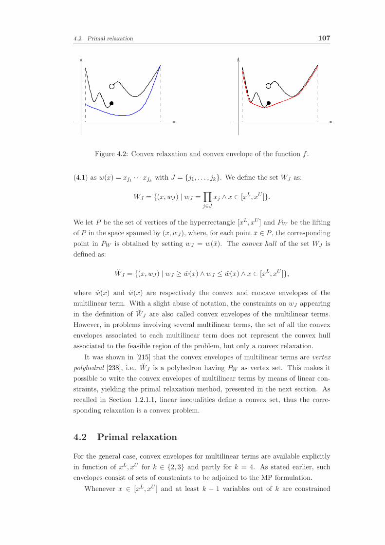
4.2. Primal relaxation 107
Figure 4.2: Convex relaxation and convex envelope of the function f .
(4.1) as w(x) = xj1 · · ·xjk with J = j1, . . . , jk. We define the set WJ as:
WJ = (x,wJ) | wJ =∏
j∈Jxj ∧ x ∈ [xL, xU ].
We let P be the set of vertices of the hyperrectangle [xL, xU ] and PW be the lifting
of P in the space spanned by (x,wJ), where, for each point x ∈ P , the correspondingpoint in PW is obtained by setting wJ = w(x). The convex hull of the set WJ is
defined as:
WJ = (x,wJ) | wJ ≥ w(x) ∧ wJ ≤ w(x) ∧ x ∈ [xL, xU ],
where w(x) and w(x) are respectively the convex and concave envelopes of the
multilinear term. With a slight abuse of notation, the constraints on wJ appearing
in the definition of WJ are also called convex envelopes of the multilinear terms.
However, in problems involving several multilinear terms, the set of all the convex
envelopes associated to each multilinear term does not represent the convex hull
associated to the feasible region of the problem, but only a convex relaxation.
It was shown in [215] that the convex envelopes of multilinear terms are vertex
polyhedral [238], i.e., WJ is a polyhedron having PW as vertex set. This makes it
possible to write the convex envelopes of multilinear terms by means of linear con-
straints, yielding the primal relaxation method, presented in the next section. As
recalled in Section 1.2.1.1, linear inequalities define a convex set, thus the corre-
sponding relaxation is a convex problem.
4.2 Primal relaxation
For the general case, convex envelopes for multilinear terms are available explicitly
in function of xL, xU for k ∈ 2, 3 and partly for k = 4. As stated earlier, such
envelopes consist of sets of constraints to be adjoined to the MP formulation.
Whenever x ∈ [xL, xU ] and at least k − 1 variables out of k are constrained

108 Chapter 4. Primal and dual convex relaxations for multilinear terms
to be integer, the corresponding multilinear term can be linearized exactly. Each
general integer variable is replaced by an aggregation of binary variables (for example
choosing the value taken by the original integer variable), and the original multilinear
term w(x) is replaced by a sum of multilinear terms with at least k − 1 binary
variables. A sequence of k − 1 Fortet’s linearizations (see Section 4.2.1.2) will then
yield a MILP formulation of the original multilinear term.
Whenever at least two variables in a multilinear term are continuous, exact
linearizations are in general no longer possible, and one must resort to solution
techniques for nonconvex programs, such as the sBB algorithm presented in Section
1.2.2.5. This involves repeatedly solving the original problem and a convex relax-
ation thereof over appropriate sets of ranges [xL, xU ]. The relaxation is obtained
by replacing each multilinear term with an added variable wJ and adjoining some
constraints to the formulation which define a convex relaxation of WJ . In general,
the tighter these relaxations are, the more efficient the sBB will be.
4.2.1 Bilinear terms
Consider now a problem having a bilinear term. For the sake of clarity, we suppose
that the two variables involved in the product are x1 and x2, and the product is
w(x1, x2) = x1x2. A graphical representation of the surface w(x1, x2) is shown in
Figure 4.3.
Figure 4.3: The bilinear surface w(x1, x2) = x1x2.

4.2. Primal relaxation 109
4.2.1.1 McCormick’s inqualities
The constraints used to define the convex envelopes for the term x1x2 are the fol-
lowing:
w1,2 ≥ xL1 x2 + xL2 x1 − xL1 xL2 (4.2)
w1,2 ≥ xU1 x2 + xU2 x1 − xU1 xU2 (4.3)
w1,2 ≤ xL1 x2 + xU2 x1 − xL1 xU2 (4.4)
w1,2 ≤ xU1 x2 + xL2 x1 − xU1 xL2 , (4.5)
where w1,2 is the new variable replacing the product x1x2. These constraints, called
McCormick inequalities, were first described in [183] and later shown to be envelopes
in [9]. Figure 4.4 shows the lower convex and upper concave envelopes for the bilinear
term x1x2. The former is defined by constraints (4.2) and (4.3), while the latter is
defined by (4.4) and (4.5).
Figure 4.4: Lower convex (left) and upper concave (right) envelopes for the bilinearterm.
4.2.1.2 Fortet inequalities
It was observed in [93, 119] that if k = 2 and x1, x2 ∈ 0, 1, then w(x) can be
replaced by an added variable w1,2 ∈ [0, 1] whilst the Fortet inequalities are adjoined
to the model:
w1,2 ≥ 0
w1,2 ≥ x1 + x2 − 1
w1,2 ≤ x1w1,2 ≤ x2,
which can be obtained by the McCormick inequalities where xL1 = xL2 = 0 and
xU1 = xU2 = 1. This reformulation is an exact linearization of the original bilinear
program [157,160] (i.e., w1,2 = 1 if and only if x1 = 1 and x2 = 1).

110 Chapter 4. Primal and dual convex relaxations for multilinear terms
4.2.2 Trilinear terms: Meyer-Floudas inequalities
Significant progress was made by Meyer and Floudas [187, 188], who were able to
write the explicit envelopes for the trilinear term w(x) = x1x2x3. Their exact form
depends on the relative sign of the variable bounds xL, xU . The cases where the
bound signs are equal are discussed in [187] (each case giving rise to 12 inequalities),
whereas the cases where the bounds have opposite signs for at least one variable
are discussed in [188]. Several of these cases also involve checking nontrivial bound
relations. Although Meyer and Floudas’ results are conceptually simple to apply
(it suffices to establish which is the case at hand, and adjoin the corresponding
inequalities to the MP), the inequalities themselves are much more involved than
McCormick’s, and it is very easy to make mistakes when integrating them in a com-
puter program. Worst of all, however, is the fact that some coefficients appearing in
Meyer-Floudas inequalities involve nontrivial floating point operations. For example,
see the coefficients c1 and c2 of x1 in (4.6) and (4.7). As is well-known, floating point
additions and subtractions are error-prone [141, 4.2.1]. This will yield an inaccurate
constraint representation of WJ ; to make things worse, as the simplex method will
identify optimal solutions at the vertices of the polyhedron, then this inaccuracy will
impact the optimal solution. In particular, if variables are constrained to be integer,
a feasible integer solution on or near the vertex of the polyhedron might be deemed
infeasible. By contrast, each coefficient of the the McCormick inequalities (k = 2)
only involves floating point multiplication, which is a much safer operation.
As example, we report the Meyer-Floudas inequalities for the case where the three
variables involved in the product have nonnegative lower (and upper) bounds [187].
To write the convex envelope, first the three variables must be mapped onto the
variables x1, x2, and x3 such that the following relationships hold:
xU1 xL2 x
L3 + xL1 x
U2 x
U3 ≤ xL1 xU2 xL3 + xU1 x
L2 x
U3
xU1 xL2 x
L3 + xL1 x
U2 x
U3 ≤ xU1 xU2 xL3 + xL1 x
L2 x
U3 .
Then, the following constraints (defining the convex envelope) have to be adjoined
to the model:
w1,2 ≥ xL2 xL3 x1 + xL1 xL3 x2 + xL1 x
L2 x3 − 2xL1 x
L2 x
L3
w1,2 ≥ xU2 xU3 x1 + xU1 xU3 x2 + xU1 x
U2 x3 − 2xU1 x
U2 x
U3
w1,2 ≥ xL2 xU3 x1 + xL1 xU3 x2 + xU1 x
L2 x3 − xL1 xL2 xU3 − xU1 xL2 xU3
w1,2 ≥ xU2 xL3 x1 + xU1 xL3 x2 + xL1 x
U2 x3 − xU1 xU2 xL3 − xL1 xU2 xL3
w1,2 ≥ c1x1 + xU1 xL3 x2 + xU1 x
L2 x3 + xL1 x
U2 x
U3 − c1xL1 − xU1 xU2 xL3 − xU1 xL2 xU3
w1,2 ≥ c2x1 + xL1 xU3 x2 + xL1 x
U2 x3 + xU1 x
L2 x
L3 − c2xU1 − xL1 xL2 xU3 − xL1 xU2 xL3 ,

4.3. Dual relaxation 111
where
c1 =xU1 x
U2 x
L3 − xL1 xU2 xU3 − xU1 xL2 xL3 + xU1 x
L2 x
U3
xU1 − xL1(4.6)
c2 =xL1 x
L2 x
U3 − xU1 xL2 xL3 − xL1 xU2 xU3 + xL1 x
U2 x
L3
xL1 − xU1. (4.7)
The concave envelope is defined by these constraints:
w1,2 ≤ xL2 xL3 x1 + xU1 xL3 x2 + xU1 x
U2 x3 − xU1 xU2 xL3 − xU1 xL2 xL3
w1,2 ≤ xU2 xL3 x1 + xL1 xL3 x2 + xU1 x
U2 x3 − xU1 xU2 xL3 − xL1 xU2 xL3
w1,2 ≤ xL2 xL3 x1 + xU1 xU3 x2 + xU1 x
L2 x3 − xU1 xL2 xU3 − xU1 xL2 xL3
w1,2 ≤ xU2 xU3 x1 + xL1 xL3 x2 + xL1 x
U2 x3 − xL1 xU2 xU3 − xL1 xU2 xL3
w1,2 ≤ xL2 xU3 x1 + xU1 xU3 x2 + xL1 x
L2 x3 − xU1 xL2 xU3 − xL1 xL2 xU3
w1,2 ≤ xU2 xU3 x1 + xL1 xU3 x2 + xL1 x
L2 x3 − xL1 xU2 xU3 − xL1 xL2 xU3 .
4.2.3 Quadrilinear terms
For quadrilinear terms, the explicit envelopes have not been found yet. A first
attempt in this direction is presented in the M.Sc. thesis of S. Balram [18], where 44
inequalities for the simplest of the quadrilinear cases (all bounds in the nonnegative
orthant) are presented. The thesis does not mention how many cases there will be
in total for k = 4, but several coefficients of this simplest case involve even more
floating point additions and subtractions than the Meyer-Floudas’ inequalities, and
are therefore expected to yield inaccurate formulations. As for the trilinear case,
when integer variables are involved, some feasible solutions might be incorrectly
deemed infeasible.
Another way to relax quadrilinear terms is to employ McCormick and Meyer-
Floudas relaxations. The associative expression for x1x2x3x4 yielding the tightest
convex relaxation is obtained by combining the convex envelope of trilinear terms
and that of bilinear terms [25, 49].
The state-of-the-art in computing envelopes for multilinear terms with k ≥ 3
involves the use of PORTA [55] (which implements the Fourier-Motzkin elimination
algorithm [70], and given specific values for xL, xU , is able to write the corresponding
constraints for the envelopes of the points in PW ) or cdd [100]. Since the resulting
inequalities change in function of the bounds, the use of this software within the
sBB algorithm, where the bounds change at each node, would be prohibitive.
4.3 Dual relaxation
The fact that the envelopes of multilinear terms are vertex polyhedral immediately
suggests the following dual approach: express a point in WJ as the convex combina-

112 Chapter 4. Primal and dual convex relaxations for multilinear terms
tion of the set PW of extreme points of WJ . We look for a vector λ of 2k nonnegative
Lagrange multipliers such that:
[x,w] =∑
i≤2k
λipi ∧∑
i≤2k
λi = 1,
where PW = p1, . . . , p2k ⊆ Rk+1. Now all that remains to do, in order to make
(4.3) explicit envelopes, is to express the pi’s in function of xL, xU . To this aim, we
define two elements: the binary 2k × k matrix D = (di,j), and the function b which
maps a binary vector of dimension k to a vector of the same dimension such that
a value of 0 (1) in position j of the input vector corresponds to the lower (upper)
bound of the variable xj in the position j of the output vector. Each row i of D is
the binary representation of the integer number i− 1 (since i starts from 1) using k
digits. In this way dij is either 0 or 1 according as to whether the j-th component
of pi is a lower or upper bound, and bj(dij) returns the correct component:
∀j ≤ k bj(0) = xLj ∧ bj(1) = xUj .
We relax the k-linear term w(x) = x1 · · ·xk as follows. We add 2k new nonneg-
atively constrained variables λi ≥ 0 (for i ≤ 2k) and k + 2 new constraints:
∀j ≤ k xj =∑
i≤2k
λibj(dij) (4.8)
w =∑
i≤2k
λi∏
j≤k
bj(dij) (4.9)
∑
i≤2k
λi = 1. (4.10)
Let WJ = (x,w, λ) | (4.8) − (4.10) ∧ λ ≥ 0. By geometry and duality in LP, the
projection of WJ on the (x,w) variables is precisely WJ .
4.3.1 Example
To better explain the dual method, suppose we want to relax the bilinear term x1x2
by replacing it with the variable w1,2, where x1 ∈ [xL1 , xU1 ] and x2 ∈ [xL2 , x
U2 ].
The matrix D is the following:
0 0
0 1
1 0
1 1
.

4.4. Comparison and numerical results 113
Applying the function b we obtain:
xL1 xL2xL1 xU2xU1 xL2xU1 xU2
.
Hence, equations (4.8)-(4.10) become:
x1 = λ1xL1 + λ2x
L1 + λ3x
U1 + λ4x
U1
x2 = λ1xL2 + λ2x
U2 + λ3x
L2 + λ4x
U2
w1,2 = λ1xL1 x
L2 + λ2x
L1 x
U2 + λ3x
U1 x
L2 + λ4x
U1 x
U2
∑
i≤4
λi = 1,
where ∀i ∈ 1, 2, 3, 4 λi ≥ 0.
4.4 Comparison and numerical results
Our tests, carried out on an Intel Xeon CPU at 2.66GHz with 24GB RAM, show
that dual relaxations can be solved faster (as the formulation size increases) than
primal relaxations, and are also more stable. We measure speed by simply solving the
primal and dual relaxations for the same original problem using CPLEX 12.2 [135],
and comparing CPU times. We define a method stable when its CPU time increase
looks empirically proportional to the increase in formulation size. Firstly we consider
NLP problems, and we solve the corresponding primal LP relaxation and dual LP
relaxation. Then we measure stability by enforcing integrality constraints on some of
the problem variables, obtaining MINLPs: this yields a primal MILP relaxation and
a dual MILP relaxation. Both are solved with CPLEX 12.2, and the CPU times are
recorded and compared. This is meant to simulate the behavior of these relaxations
in a BB setting. It turns out that the running times of the MILP solver on the dual
MILP relaxation is proportional to the relaxation size, whereas it varies wildly for
the primal MILP relaxation.
We generated 2520 random multilinear nonseparable NLPs, involving linear, bi-
linear, and trilinear terms. For each such NLP P , we generated the primal LP
relaxation RP and the dual LP relaxation ΛP . Then we set some variables of the
previously generated NLPs to be integer, thus obtaining MINLPs, and for each
MINLP P , we generated the primal MILP relaxation R′P and the dual MILP re-
laxation Λ′P . We let n (the number of original variables) vary in 10, 20. For
n = 10 we let the number of bilinear terms β vary in 0, 10, 13, 17, 21, 25, 29, 33and of trilinear terms τ in 0, 10, 22, 34, 36, 58, 71, 83. For n = 20, we let β vary
in 0, 20, 38, 57, 76, 95, 114, 133 and τ in 0, 20, 144, 268, 393, 517, 642, 766. Note

114 Chapter 4. Primal and dual convex relaxations for multilinear terms
that the total number of combinations of (n, β, τ), given n, is 63, because the case
β = τ = 0 is excluded. For each combination of the triplet (n, β, τ) we generated 20
random instances. In summary, we have 63 combinations for each value of n, and
we have two values of n (that is, 10 and 20) For each case we generated 20 random
instances, and we obtain a total of 63 · 2 · 20 = 2520 random instances. The variable
bounds, chosen at random, were all of magnitude ±1× 20.
The CPU time results (in seconds) comparing RP ,ΛP are given in Figures 4.5-
4.6. The horizontal axis is marked by the instance ID. Each recognizable “block”
corresponds to a fixed value of β. Since bilinear terms give rise to fewer relaxation
variables/constraints than trilinear ones, the formulation size is strongly proportional
to τ and weakly proportional to β. The CPU time results (in seconds) comparing
R′P ,Λ
′P are given in Figures 4.7-4.8.
0 10 20 30 40 50 600
0.005
0.01
0.015
0.02
0.025
instance set
CP
U ti
me
[s]
primal relaxationdual relaxation
Figure 4.5: CPU time averages (in seconds) over each 20-instance set with given(n, β, τ) with n = 10 for the LP relaxations.
4.5 Conclusions
From the cases k = 3 and k = 4 it appears clearly that the explicit form of the
inequalities describing WJ , in function of xL, xU , considerably increases in com-
plexity (from the point of view of floating point additions and subtractions) as k
increases, thereby causing numerical instability. But this is not all: the number of
such inequalities, even when they are found explicitly with PORTA, also increases,
thereby yielding ever more sizable formulations. While it is known that this number
increases as O(2k), the first column of Table 4.1 suggests that the increase is more
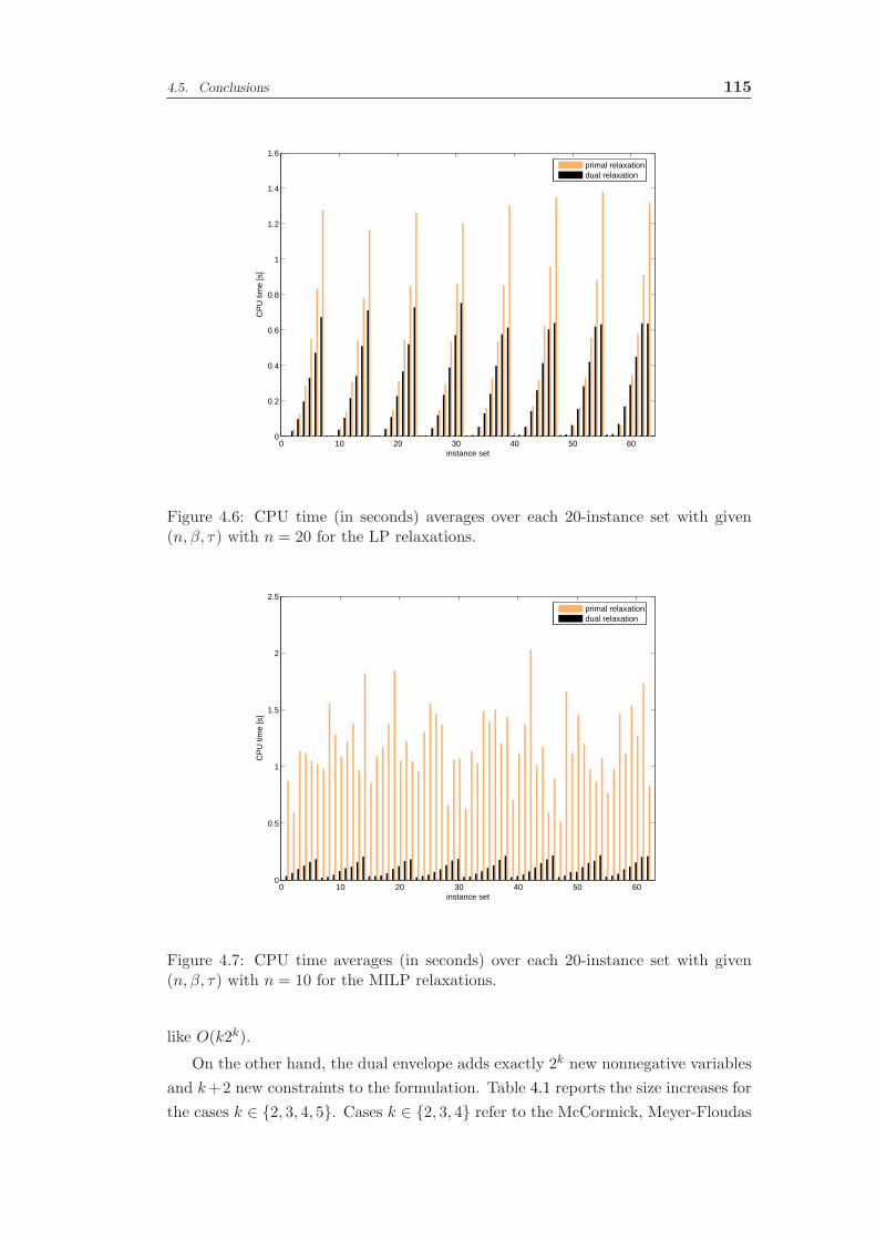
4.5. Conclusions 115
0 10 20 30 40 50 600
0.2
0.4
0.6
0.8
1
1.2
1.4
1.6
instance set
CP
U ti
me
[s]
primal relaxationdual relaxation
Figure 4.6: CPU time (in seconds) averages over each 20-instance set with given(n, β, τ) with n = 20 for the LP relaxations.
0 10 20 30 40 50 600
0.5
1
1.5
2
2.5
instance set
CP
U ti
me
[s]
primal relaxationdual relaxation
Figure 4.7: CPU time averages (in seconds) over each 20-instance set with given(n, β, τ) with n = 10 for the MILP relaxations.
like O(k2k).
On the other hand, the dual envelope adds exactly 2k new nonnegative variables
and k+2 new constraints to the formulation. Table 4.1 reports the size increases for
the cases k ∈ 2, 3, 4, 5. Cases k ∈ 2, 3, 4 refer to the McCormick, Meyer-Floudas

116 Chapter 4. Primal and dual convex relaxations for multilinear terms
0 10 20 30 40 50 600
100
200
300
400
500
600
700
800
900
instance set
CP
U ti
me
[s]
primal relaxationdual relaxation
Figure 4.8: CPU time averages (in seconds) over each 20-instance set with given(n, β, τ) with n = 20 for the MILP relaxations.
and Balram [18] inequalities. The statistic for k = 5 is taken from [18], but devised
computationally using a method similar to PORTA.
k Primal Dual
2 4 83 12 134 44 225 130 39
Table 4.1: Per-multilinear-term size increase (new constraints and variables) forprimal and dual envelopes.
Numerical results confirm this behavior. Considering LP problems, although
for n = 10 (see Figure 4.5) the CPU time is very slightly in favor of the primal
relaxation, the situation changes visibly for n = 20 (see Figure 4.6). However, even
if the CPU times differ, we cannot infer much on the comparative stability of the
two methods.
Moving to the MILP problems, the CPU differences are decidedly striking in
the case n = 10 and even excessively so for the case n = 20, as shown in Figures
4.7 and 4.8. The CPU time taken to solve primal relaxations is far from propor-
tional to formulation size, whereas the stability associated to the dual relaxation is
remarkable.

Part IV
Conclusions and bibliography


Chapter 5Conclusions
The main aim of this thesis is to convince the reader about the importance of re-
formulations in MP, both from a theoretical and a practical point of view. As a
matter of fact, very often the most natural formulation to describe a problem is not
the most efficient to be solved, and better results (for example in terms of com-
putational time to get the optimal solution) can be achieved by reformulating the
original model. It turns out that to perform this reformulation step in a profitable
way one should know how the solvers work and what is the relationship (even ap-
proximately) between the kind of problem to solve (e.g., LP, MILP, NLP) and its
complexity. This is very important to have somehow an “intuition” toward the best
formulation, and to avoid reformulations that are harder to solve than the original
formulation. For example, if one artificially reformulates a LP problem to a NLP
problem, it is very likely that finding an optimal solution will take longer. This is the
reason why in Chapter 1 we reported a short description of the different categories
of MP problems (with some order relationships on their complexities) and solvers.
However, there can be cases where it is not clear, before performing some numerical
experiments, which, between the original formulation and a reformulation, is best.
Consider for example the reformulation proposed in Chapter 3, where we replaced
the constraints (2.22)-(2.23) with the constraints (2.34)-(2.35). It is not so obvious
that the second set of inequalities is better than the first set, but some tests con-
firmed this fact. However, we tried to give an explanation of this behavior on the
basis of our knowledge about the used solver.
In this thesis we followed the classification proposed by Liberti in [157]: exact
reformulations, narrowings, and relaxations. Basically, each case corresponds to a
chapter where we presented a problem and its MP formulation. Then we derived
reformulations, motivated by a theoretical analysis of the problem. The order of
presentation of the reformulations is related to a logical interpretation of the solu-
tion process of a difficult problem: starting from the original formulation, one can
employ an exact reformulation, that does not alter the set of optimal solutions. If

120 Chapter 5. Conclusions
the problem is still difficult to solve, and it presents symmetries, narrowings refor-
mulation can be used to make some optimal solutions infeasible with the guarantee
that at least one is preserved. Finally, if the other techniques fail, one can relax
the problem. This means that the solution of the corresponding relaxation does not
provide the optimal solution of the original problem, but a lower (upper) bound in
case of an objective function being minimized (maximized).
Chapter 2 deals with exact reformulations, and the problem studied is the clus-
tering by means of modularity maximization. Actually in that chapter we also
introduced another problem related to clustering, that can be described by means
of MP, but due to the size of the resulting formulation we decided to implement a
specific (as opposed to general-purpose) BB algorithm to solve it. However, con-
cerning the modularity maximization problem, we considered a heuristic that solves
a cMIQP problem at each step. We proposed some reformulations of this cMIQP
formulation, that are basically compact models where we were able to decrease the
number of variables and constraints by preserving the optimal solutions set. More-
over, the theoretical analysis underlined a symmetric structure of the problem, thus
we also employed a SBC, yielding a narrowing (which is the main subject of Chapter
3). Thanks to these reformulations, the computational time to solve some classical
instances by the heuristic was decreased by an order of magnitude. We also consid-
ered the extension of this method to bipartite graphs, and the MP model in this case
in not a cMIQP but a MINLP, hence it is more difficult to solve. It is interesting
to notice that the reformulation techniques yielding the best results for unipartite
graphs are not the same as for bipartite graphs, even if the problems are strictly
related. By the way, one of the reformulations used for the bipartite case (that
is (2.101)-(2.108)) was really close to the original formulation for the general case,
thus underlying the strict relationship between these problems. This was not clear
by comparing the original formulations.
In Chapter 3 we studied the problem of packing equal circles in a square. As
this problem involves a high degree of symmetries, it is a very good candidate for
the application of narrowings. We were able to characterize the symmetric structure
of the problem, and then to obtain some SBCs in an automatic way. Furthermore
we derived some other SBCs that are more effective than the ones obtained auto-
matically, in the sense that they lead to an improvement of the bounds provided
by the sBB, giving good quality solutions already at the root of the sBB tree. We
also proposed some other valid inequalities and finally we presented a conjecture
about the reduction of the range for some variables of the problem. This last point
is motivated by the fact that in the original formulation all the variables have the
same range, and this causes a very poor relaxation of the problem (as computed at
the root node of the sBB tree).
Finally, in Chapter 4 we compared two relaxations for problems involving mul-
tilinear terms. The first, called primal, defines the convex relaxation of the problem

121
using a set of inequalites. The second one, called dual, represents the convex relax-
ation as the convex combination of the vertices of the convex hull using dual variables
λ. The optimal solutions of these relaxations is the same for a given problem, thus
we could say that one is an exact reformulation of the other. These relaxations are
known in the literature, and usually the primal is the most used. We showed that
for NLPs, and still more for MINLPs, the dual approach outperforms the primal in
terms of computational time and size of the formulation.
It appears that the problems we studied are very different, but in every case we
had some advantages by applying reformulation techniques. This is an indication
of the fact that given a general problem, it is worth to spend some time to study it
and to try to improve the original formulation.
The future work has two main directions. First, to perform an analysis of the
different reformulation techniques which can be used fo a general problem. It is
not easy, as the efficacy of the reformulations is very often related to the specific
problem. However, we have some examples in this thesis, as the constraints (2.34)-
(2.35) which in case of maximization problems can be used in place of (2.22)-(2.23),
or the automatic symmetry detection techniques presented in Chapter 3. Second,
once these reformulations techniques are formalized, to integrate them in a solver.
Indeed this is a hard task, because the human analysis of the problem can detect
some particular features of a problem that are difficult to find automatically, but
its importance is crucial, above all in Operations Research where very often a user
models a problem having only a limited knowledge about the solution process and
without trying to improve the first formulation obtained.

122 Chapter 5. Conclusions

Bibliography
[1] K. Abhishek, S. Leyffer, and J. Linderoth. FilMINT: An Outer Approximation-
Based Solver for Convex Mixed-Integer Nonlinear Programs. INFORMS Jour-
nal on Computing, 22(4):555–567, 2010.
[2] W. P. Adams and P. M. Dearing. On the equivalence between roof duality and
Lagrangian duality for unconstrained 0− 1 quadratic programming problems.
Discrete Applied Mathematics, 48(1):1–20, 1994.
[3] B. Addis, M. Locatelli, and F. Schoen. Disk Packing in a Square: A New
Global Optimization Approach. INFORMS Journal on Computing, 20(4):516–
524, 2008.
[4] N. Adhya, M. Tawarmalani, and N. V. Sahinidis. A Lagrangian Approach
to the Pooling Problem. Industrial & Engineering Chemistry Research,
38(5):1956–1972, 1999.
[5] C. S. Adjiman, S. Dallwig, C. A. Floudas, and A. Neumaier. A global opti-
mization method, αBB, for general twice-differentiable constrained NLPs: I.
Theoretical advances. Computers & Chemical Engineering, 22(9):1137–1158,
1998.
[6] G. Adomavicius and A. Tuzhilin. Toward the next generation of recommender
systems: A survey of the state-of-the-art and possible extensions. IEEE Trans-
actions on Knowledge and Data Engineering, 17(6):734–749, 2005.
[7] A. Agarwal, S. Bhat, A. Gray, and I. E. Grossmann. Automating Mathematical
Program Transformations. In M. Carro and R. Pena, editors, Proceedings of the
12th International Symposium on Practical Aspects of Declarative Languages
(PADL), volume 5937 of Lecture Notes in Computer Science, pages 134–148.
Springer Berlin / Heidelberg, 2010.
[8] G. Agarwal and D. Kempe. Modularity-Maximizing Graph Communities via
Mathematical Programming. The European Physical Journal B, 66(3):409–
418, 2008.

124 Bibliography
[9] F. Al-Khayyal and J. Falk. Jointly Constrained Biconvex Programming. Math-
ematics of Operations Research, 8(2):273–286, 1983.
[10] D. Aloise, S. Cafieri, G. Caporossi, P. Hansen, S. Perron, and L. Liberti.
Column generation algorithms for exact modularity maximization in networks.
Physical Review E, 82(4):046112, 2010.
[11] K. Anstreicher. Semidefinite programming versus the reformulation-
linearization technique for nonconvex quadratically constrained quadratic pro-
gramming. Journal of Global Optimization, 43(2):471–484, 2009.
[12] D. L. Applegate, R. E. Bixby, V. Chvatal, and W. J. Cook. The Traveling
Salesman: a Computational Study. Princeton University Press, Princeton,
2007.
[13] A. Arenas, A. Fernandez, and S. Gomez. Analysis of the structure of complex
networks at different resolution levels. New Journal of Physics, 10(5):053039,
2008.
[14] C. Audet, J. Brimberg, P. Hansen, S. Le Digabel, and N. Mladenovic. Pool-
ing Problem: Alternate Formulations and Solution Methods. Management
Science, 50(6):761–776, 2004.
[15] C. Audet, P. Hansen, B. Jaumard, and G. Savard. Links between linear bilevel
and mixed 0− 1 programming problems. Journal of Optimization Theory and
Applications, 93(2):273–300, 1997.
[16] M. Avriel and B. Golany. Mathematical Programming for Industrial Engineers.
Marcel Dekker, 1996.
[17] B. Ball, B. Karrer, and M. E. J. Newman. Efficient and principled method for
detecting communities in networks. Physical Review E, 84(3):036103, 2011.
[18] S. Balram. Crude transshipment via floating, production, storage and offload-
ing platforms. Master’s thesis, Deptartment of Chemical and Biomolecular
Engineering, National University of Singapore, 2010.
[19] M. J. Barber. Modularity and community detection in bipartite networks.
Physical Review E, 76(6):066102, 2007.
[20] M. J. Barber and J. W. Clark. Detecting network communities by propagating
labels under constraints. Physical Review E, 80(2):026129, 2009.
[21] C. Barnhart and G. Laporte, editors. Transportation, volume 14 of Handbooks
in Operations Research and Management Science. North-Holland, Amsterdam,
2007.

Bibliography 125
[22] V. Batagelj and A. Mrvar. Pajek datasets, 2006.
[23] S. Bazaraa, H. D. Sherali, and C. M. Shetty. Nonlinear Programming: Theory
and Algorithms. Wiley-Interscience, 2006.
[24] P. Belotti, S. Cafieri, J. Lee, and L. Liberti. Feasibility-based bounds tight-
ening via fixed points. In D.-Z. Du, P. M. Pardalos, and B. Thuraisingham,
editors, Proceedings of the 4th International Conference on Combinatorial Op-
timization and Applications (COCOA), volume 6508 of Lecture Notes in Com-
puter Science, pages 65–76. Springer, New York, 2010.
[25] P. Belotti, S. Cafieri, J. Lee, L. Liberti, and A. Miller. On the composition
of convex envelopes for quadrilinear terms. In P. M. Pardalos, editor, Opti-
mization and Optimal Control, Nonconvex Optimization and Its Application.
Springer, New York, to appear.
[26] P. Belotti, J. Lee, L. Liberti, F. Margot, and A. Wachter. Branching and
bounds tightening techniques for non-convex MINLP. Optimization Methods
and Software, 24(4-5):597–634, 2009.
[27] A. Ben-Israel and B. Mond. What is invexity? Journal of Australian Mathe-
matical Society B, 28(1):1–9, 1986.
[28] L. Bertacco, M. Fischetti, and A. Lodi. A feasibility pump heuristic for general
mixed-integer problems. Discrete Optimization, 4(1):63–76, 2007.
[29] T. Berthold and A. Gleixner. Undercover — Primal MINLP Heuristic. In
P. Bonami, L. Liberti, A. Miller, and A. Sartenaer, editors, Proceedings of the
European Workshop on Mixed-Integer Nonlinear Programming (EWMINLP),
pages 103–113. Universite de la Mediterranee, Marseille, 2010.
[30] R. E. Bixby. Solving Real-World Linear Programs: A Decade and More of
Progress. Operations Research, 50(1):3–15, 2002.
[31] S. Boccaletti, M. Ivanchenko, V. Latora, A. Pluchino, and A. Rapisarda. De-
tecting complex network modularity by dynamical clustering. Physical Review
E, 75(4):045102, 2007.
[32] D. W. Boll, J. Donovan, R. L. Graham, and B. D. Lubachevsky. Improving
Dense Packings of Equal Disks in a Square. Electronic Journal of Combina-
torics, 7(1, R46):1–9, 2000.
[33] M. Bolla. Penalized versions of the Newman-Girvan modularity and their
relation to normalized cuts and k-means clustering. Physical Review E,
84(1):016108, 2011.

126 Bibliography
[34] P. Bonami, G. Cornuejols, A. Lodi, and F. Margot. A Feasibility Pump for
mixed integer nonlinear programs. Mathematical Programming, 119(2):331–
352, 2009.
[35] P. Bonami and J. P. M. Goncalves. Primal heuristics for mixed integer non-
linear programs. Technical Report RC24639, IBM, 2008.
[36] P. Bonami and J. Lee. BONMIN user’s manual. Technical report, IBM, June
2007.
[37] M. Boulle. Compact Mathematical Formulation for Graph Partitioning. Op-
timization and Engineering, 5(3):315–333, 2004.
[38] S. Bradley, A. Hax, and T. Magnanti. Applied Mathematical Programming.
Addison Wesley, 1977.
[39] U. Brandes, D. Delling, M. Gaertler, R. Gorke, M. Hoefer, Z. Nikoloski, and
D. Wagner. On Modularity Clustering. IEEE Transactions on Knowledge and
Data Engineering, 20(2):172–188, 2008.
[40] H. Breu and D. Kirkpatrick. On the complexity of recognizing intersection and
touching graphs of disks. In F. Brandenburg, editor, Graph Drawing, volume
1027 of Lecture Notes in Computer Science, pages 88–98. Springer, Berlin,
1996.
[41] J. Brimberg, P. Hansen, N. Mladenovic, and E. Taillard. Improvement and
Comparison of Heuristics for Solving the Uncapacitated Multisource Weber
Problem. Operations Research, 48(3):444–460, 2000.
[42] A. Brook, D. Kendrick, and A. Meeraus. GAMS, a user’s guide. ACM
SIGNUM Newsletter, 23(3-4):10–11, 1988.
[43] G. G. Brown and R. F. Dell. Formulating integer linear programs: A rogues’
gallery. INFORMS Transactions on Education, 7:1–13, 2007.
[44] S. Cafieri, G. Caporossi, P. Hansen, S. Perron, and A. Costa. Finding com-
munities in networks in the strong and almost-strong sense. Physical Review
E, 85(4):046113, 2012.
[45] S. Cafieri, A. Costa, and P. Hansen. Reformulation of a model for hierarchical
divisive graph modularity maximization. Annals of Operations Research, in
revision.
[46] S. Cafieri, P. Hansen, and L. Liberti. Loops and multiple edges in modularity
maximization of networks. Physical Review E, 81(4):046102, 2010.
[47] S. Cafieri, P. Hansen, and L. Liberti. Locally optimal heuristic for modularity
maximization of networks. Physical Review E, 83(5):056105, 2011.

Bibliography 127
[48] S. Cafieri, P. Hansen, and L. Liberti. Improving heuristics for network modu-
larity maximization using an exact algorithm. Discrete Applied Mathematics,
to appear.
[49] S. Cafieri, J. Lee, and L. Liberti. On convex relaxations of quadrilinear terms.
Journal of Global Optimization, 47(4):661–685, 2010.
[50] G. Caporossi and P. Hansen. Variable neighborhood search for extremal
graphs: 1 The AutoGraphiX system. Discrete Mathematics, 212(1-2):29–44,
2000.
[51] L. Casado, I. Garcıa, P. Szabo, and T. Csendes. Equal circles packing in
square II: new results for up to 100 circles using the TAMSASS-PECS algo-
rithm. In F. Giannessi, P. M. Pardalos, and T. Rapcsak, editors, Optimization
Theory: Recent Developments from Matrahaza, pages 207–224. Kluwer, Dor-
drecht, 2001.
[52] I. Castillo, F. Kampas, and J. Pinter. Solving circle packing problems by
global optimization: Numerical results and industrial applications. European
Journal of Operational Research, 191(3):786–802, 2008.
[53] B. Chachuat. Nonlinear and Dynamic Optimization: From Theory to Practice.
Automatic Control Laboratory, EPFL, Switzerland, 2007.
[54] P. K. Chan, M. D. F. Schlag, and J. Y. Zien. Spectral K-way ratio-cut parti-
tioning and clustering. IEEE Transactions on CAD of Integrated Circuits and
Systems, 13(9):1088–1096, 1994.
[55] T. Christof and A. Lobel. The porta manual page. Technical Report v. 1.4.0,
ZIB, Berlin, 1997.
[56] V. Chvatal. Linear Programming. Series of Books in the Mathematical Sci-
ences. W. H. Freeman, 1983.
[57] A. Clauset, M. E. J. Newman, and C. Moore. Finding community structure
in very large networks. Physical Review E, 70(6):066111, 2004.
[58] A. Costa and P. Hansen. Comment on “Evolutionary method for finding com-
munities in bipartite networks”. Physical Review E, 84(5):058101, 2011.
[59] A. Costa, P. Hansen, and L. Liberti. Static symmetry breaking in circle pack-
ing. In U. Faigle, R. Schrader, and D. Herrmann, editors, Proceedings of
the 9th Cologne-Twente Workshop on Graphs and Combinatorial Optimiza-
tion (CTW), pages 47–50. University of Koln, 2010.
[60] A. Costa, P. Hansen, and L. Liberti. Bound constraints for Point Packing
in a Square. In L. Adacher, M. Flamini, G. Leo, G. Nicosia, A. Pacifici,

128 Bibliography
and V. Piccialli, editors, Proceedings of the 10th Cologne-Twente Workshop on
Graphs and Combinatorial Optimization (CTW), pages 126–129. Universita di
Roma “Tor Vergata”, Villa Mondragone, 2011.
[61] A. Costa, P. Hansen, and L. Liberti. On the impact of symmetry-breaking con-
straints on spatial Branch-and-Bound for circle packing in a square. Discrete
Applied Mathematics, 161(1-2):96–106, 2013.
[62] A. Costa and L. Liberti. Relaxations of Multilinear Convex Envelopes: Dual
Is Better Than Primal. In R. Klasing, editor, Proceedings of the 11th Interna-
tional Symposium on Experimental Algorithms (SEA), volume 7276 of Lecture
Notes in Computer Science, pages 87–98. Springer, 2012.
[63] A. Costa, L. Liberti, and P. Hansen. Formulation symmetries in circle packing.
In A. R. Mahjoub, editor, Proceedings of the 1st International Symposium on
Combinatorial Optimization (ISCO), volume 36 of Electronic Notes in Discrete
Mathematics, pages 1303–1310. Elsevier, 2010.
[64] A. Costa and I. Tseveendorj. Symmetry breaking constraints for the problem
of packing equal circles in a square. In C. J. Luz and F. Valente, editors,
Proceedings of the 1st International Conference on Operations Research and
Enterprise Systems (ICORES), pages 5–10. SciTePress, 2012.
[65] B. D. Craven and B. M. Glover. Invex functions and duality. Journal of the
Australian Mathematical Society A, 39(1):1–20, 1985.
[66] Y. Cui. Generating optimal t-shape cutting patterns for circular blanks. Com-
puters & Operations Research, 32(1):143–152, 2005.
[67] C. D’Ambrosio, J. Linderoth, and J. Luedtke. Valid Inequalities for the Pooling
Problem with Binary Variables. In O. Gunluk and G. Woeginger, editors,
Proceedings of the 15th Integer Programming and Combinatorial Optimization
Conference (IPCO), volume 6655 of Lecture Notes in Computer Science, pages
117–129. Springer / Heidelberg, 2011.
[68] E. Danna, E. Rothberg, and C. Le Pape. Exploring relaxation induced neigh-
borhoods to improve MIP solutions. Mathematical Programming, 102(1):71–
90, 2005.
[69] L. Danon, A. Dıaz-Guilera, and A. Arenas. The effect of size heterogene-
ity on community identification in complex networks. Journal of Statistical
Mechanics: Theory and Experiment, 2006(11):P11010, 2006.
[70] G. B. Dantzig. Linear Programming and Extensions. Princeton University
Press, Princeton, 1963.

Bibliography 129
[71] L. Dartnell, E. Simeonidis, M. Hubank, S. Tsoka, I. D. L. Bogle, and L. G.
Papageorgiou. Robustness of the p53 network and biological hackers. FEBS
letters, 579(14):3037–3042, 2005.
[72] T. Davidovic, L. Liberti, N. Maculan, and N. Mladenovic. Towards the optimal
solution of the multiprocessor scheduling problem with communication delays.
In P. Baptiste, G. Kendall, A. Munier-Kordon, and F. Sourd, editors, Pro-
ceedings of the 3rd Multidisciplinary International Conference on Scheduling:
Theory and Applications (MISTA), pages 128–135, Paris, 2007.
[73] A. Davis, B. B. Gardner, and M. R. Gardner. Deep South: A Social An-
thropological Study of Caste and Class. University of Chicago Press, Chicago,
1941.
[74] P. J. Davis. Packing inequalities for circles. Michigan Mathematical Journal,
10(1):25–31, 1963.
[75] E. Demaine, S. Fekete, and R. Lang. Circle packing for origami design is
hard. In A. K. Peters, editor, Proceedings of the 5th International Conference
on Origami in Science, Mathematics and Education (OSME), pages 609–626,
Singapore, 2010.
[76] T. N. Dinh and M. T. Thai. Finding Community Structure with Performance
Guarantees in Complex Networks. Technical report, arXiv:1108.4034, 2011.
[77] H. N. Djidjev. A Scalable Multilevel Algorithm for Graph Clustering and
Community Structure Detection. In W. Aiello, A. Broder, J. Janssen, and
E. Milios, editors, Proceedings of the 4th Workshop on Algorithms and Mod-
els for the Web-Graph (WAW), volume 4936 of Lecture Notes in Computer
Science, pages 117–128. Springer Berlin / Heidelberg, 2008.
[78] C. O. Dorso and A. D. Medus. Community Detection in Networks. Interna-
tional Journal of Bifurcation and Chaos, 20(2):361–367, 2010.
[79] O. du Merle, P. Hansen, B. Jaumard, and N. Mladenovic. An Interior Point Al-
gorithm for Minimum Sum-of-Squares Clustering. SIAM Journal on Scientific
Computing, 21(4):1485–1505, 2000.
[80] J. Duch and A. Arenas. Community detection in complex networks using
extremal optimization. Physical Review E, 72(2):027104, 2005.
[81] M. A. Duran and I. E. Grossmann. An outer-approximation algorithm for
a class of mixed-integer nonlinear programs. Mathematical Programming,
36(3):307–339, 1986.
[82] P. Eades and N. Wormald. Fixed edge-length graph drawing is NP-hard.
Discrete Applied Mathematics, 28(2):111–134, 1990.

130 Bibliography
[83] J. E. Falk and R. M. Soland. An Algorithm for Separable Nonconvex Pro-
gramming Problems. Management Science, 15(9):550–569, 1969.
[84] N. Fan and P. M. Pardalos. Linear and quadratic programming approaches
for the general graph partitioning problem. Journal of Global Optimization,
48(1):57–71, 2010.
[85] R. R. Faulkner. Music on Demand: Composers and Careers in the Hollywood
Film Industry. Transaction Publishers, 2003.
[86] M. C. Ferris, J. Lim, and D. M. Shepard. An Optimization Approach for
Radiosurgery Treatment Planning. SIAM Journal on Optimization, 13(3):921–
937, 2002.
[87] M. Fischetti. Lezioni di Ricerca Operativa. Edizioni Libreria Progetto Padova,
second edition, 1999.
[88] M. Fischetti, F. Glover, and A. Lodi. The feasibility pump. Mathematical
Programming, 104(1):91–104, 2005.
[89] M. Fischetti and A. Lodi. Local branching. Mathematical Programming, 98(1-
3):23–37, 2005.
[90] G. W. Flake, S. Lawrence, C. L. Giles, and F. M. Coetzee. Self-Organization
and Identification of Web Communities. IEEE Computer, 35(3):66–71, 2002.
[91] C. A. Floudas. Deterministic Global Optimization: Theory, Methods and Ap-
plications. Kluwer Academic Publishers, Dordrecht, 2000.
[92] C. A. Floudas and P. M. Pardalos, editors. Encyclopedia of Optimization.
Springer, New York, second edition, 2009.
[93] R. Fortet. Applications de l’algebre de Boole en recherche operationelle. Revue
Francaise d’Informatique et de Recherche Operationelle, 4(14):17–26, 1960.
[94] S. Fortunato. Community detection in graphs. Physics Reports, 486(3-5):75 –
174, 2010.
[95] S. Fortunato and M. Barthelemy. Resolution limit in community detection.
Proceedings of the National Academy of Sciences of the U.S.A., 104(1):36–41,
2007.
[96] L. R. Foulds, D. Haughland, and K. Jornsten. A Bilinear Approach to the
Pooling Problem. Optimization, 24(1-2):165–180, 1992.
[97] R. Fourer and D. Gay. The AMPL Book. Duxbury Press, Pacific Grove, 2002.
Bibliography 131
[98] R. J. Fowler, M. Paterson, and S. Tanimoto. Optimal packing and covering
in the plane are NP-complete. Information Processing Letters, 12(3):133–137,
1981.
[99] H. J. Fraser and J. A. George. Integrated container loading software for pulp
and paper industry. European Journal of Operational Research, 77(3):466–474,
1994.
[100] K. Fukuda and A. Prodon. Double description method revisited. In M. Deza,
R. Euler, and Y. Manoussakis, editors, proceedings of the 8th Franco-Japanese
and 4th Franco-Chinese Conference on Combinatorics and Computer Science
(CCS), volume 1120 of Lecture Notes in Computer Science, pages 91–111.
Springer, London, 1995.
[101] M. R. Garey and D. S. Johnson. Computers and Intractability: A Guide to
the Theory of NP-Completeness. Freeman and Company, New York, 1979.
[102] A. M. Geoffrion. Generalized Benders decomposition. Journal of Optimization
Theory and Applications, 10(4):237–260, 1972.
[103] J. A. George, J. M. George, and B. W. Lamar. Packing different-sized cir-
cles into a rectangular container. European Journal of Operational Research,
84(3):693–712, 1995.
[104] P. Gill. User’s guide for SNOPT version 7. Systems Optimization Laboratory,
Stanford University, California, 2006.
[105] M. Girvan and M. E. J. Newman. Community structure in social and biological
networks. Proceedings of the National Academy of Sciences of the U.S.A.,
99(12):7821–7826, 2002.
[106] F. Glover and G. Kochenberger, editors. Handbook of Metaheuristics. Kluwer,
Dordrecht, 2003.
[107] R. E. Gomory. Outline of an algorithm for integer solutions to linear programs.
Bulletin of the American Mathematical Society, 64(5):275–278, 1958.
[108] B. H. Good, Y.-A. de Montjoye, and A. Clauset. Performance of modularity
maximization in practical contexts. Physical Review E, 81(4):046106, 2010.
[109] E. Goubault, S. Le Roux, J. Leconte, L. Liberti, and F. Marinelli. Static
analysis by abstract interpretation: a mathematical programming approach.
In A. Mine and E. Rodrıguez-Carbonell, editors, Proceeding of the 2nd Inter-
national Workshop on Numerical and Symbolic Abstract Domains (NSAD),
volume 267(1) of Electronic Notes in Theoretical Computer Science, pages 73–
87. Elsevier, 2010.

132 Bibliography
[110] R. L. Graham and B. D. Lubachevsky. Repeated Patterns of Dense Packings of
Equal Disks in a Square. Electronic Journal of Combinatorics, 3(1, R16):1–17,
1996.
[111] I. E. Grossmann, J. A. Caballero, and H. Yeomans. Mathematical program-
ming approaches to the synthesis of chemical process systems. Korean Journal
of Chemical Engineering, 16(4):407–426, 1999.
[112] A. Grosso, A. R. M. J. U. Jamali, M. Locatelli, and F. Schoen. Solving the
problem of packing equal and unequal circles in a circular container. Journal
of Global Optimization, 47(1):63–81, 2010.
[113] A. Grosso, M. Locatelli, and F. Schoen. Solving molecular distance geometry
problems by global optimization algorithms. Computational Optimization and
Applications, 43(1):23–27, 2009.
[114] M. Grotschel and Y. Wakabayashi. A cutting plane algorithm for a clustering
problem. Mathematical Programming, 45(1-3):59–96, 1989.
[115] R. Guimera and L. A. N. Amaral. Functional cartography of complex
metabolic networks. Nature, 433(7028):895–900, 2005.
[116] O. K. Gupta and A. Ravindran. Branch and Bound Experiments in Con-
vex Nonlinear Integer Programming. Management Science, 31(12):1533–1546,
1985.
[117] Gurobi Optimization Inc. Gurobi Optimizer Reference Manual, 2012.
[118] L. Hagen and A. B. Kahng. New spectral methods for ratio cut partitioning
and clustering. IEEE Transactions on CAD of Integrated Circuits and Systems,
11(9):1074–1085, 1992.
[119] P. Hammer and S. Rudeanu. Boolean Methods in Operations Research and
Related Areas. Springer, Berlin, 1968.
[120] P. Hansen, J. Brimberg, N. Mladenovic, and D. Urosevic. Primal-dual variable
neighborhood search for the simple plant-location problem. INFORMS Journal
on Computing, 19(4):552–564, 2007.
[121] P. Hansen and B. Jaumard. Cluster analysis and mathematical programming.
Mathematical Programming, 79(1-3):191–215, 1997.
[122] M. A. Hanson. On sufficiency of the Kuhn-Tucker conditions. Journal of
Mathematical Analysis and Applications, 80(2):545–550, 1981.
[123] M. A. Hanson. Invexity and the Kuhn-Tucker Theorem. Journal of Mathe-
matical Analysis and Applications, 236(2):594–604, 1999.

Bibliography 133
[124] C. A. Haverly. Studies of the behaviour of recursion for the pooling problem.
ACM SIGMAP Bulletin, 25:19–28, 1978.
[125] J. Herskovits, P. Mappa, E. Goulart, and C. M. Mota Soares. Mathemati-
cal programming models and algorithms for engineering design optimization.
Computer Methods in Applied Mechanics and Engineering, 194(30-33):3244–
3268, 2005.
[126] M. Hifi and R. M’Hallah. Approximate algorithms for constrained circular
cutting problems. Computers & Operations Research, 31(5):675–694, 2004.
[127] M. Hifi and R. M’Hallah. A Literature Review on Circle and Sphere Pack-
ing Problems: Models and Methodologies. Advances in Operations Research,
2009:150624, 2009.
[128] M. Hifi, V. Th. Paschos, and V. Zissimopoulos. A simulated annealing ap-
proach for the circular cutting problem. European Journal of Operational
Research, 159(2):430–448, 2004.
[129] D. S. Hochbaum andW. Maass. Approximation schemes for covering and pack-
ing problems in image processing and VLSI. Journal of the ACM, 32(1):130–
136, 1985.
[130] E. Hopper and B. Turton. Application of genetic algorithms to packing prob-
lems - a review. In P. K. Chawdry, R. Roy, and R. K. Kant, editors, Proceedings
of the 2nd On-line World Conference of Soft Computing in Engineering Design
and Manufacturing, pages 279–288. Springer, Berlin, 1997.
[131] R. Horst and N. V. Thoai. Dc programming: Overview. Journal of Optimiza-
tion Theory and Applications, 103(1):1–43, 1999.
[132] Y. Hu, H. Chen, P. Zhang, M. Li, Z. Di, and Y. Fan. Comparative definition
of community and corresponding identifying algorithm. Physical Review E,
78(2):026121, 2008.
[133] W. Huang and T. Ye. Greedy vacancy search algorithm for packing equal
circles in a square. Operations Research Letters, 38(5):378–382, 2010.
[134] V. Hugo. Les Miserables. Gallimard, Bibliotheque de la Pleiade, Paris, 1951.
[135] IBM. ILOG CPLEX 12.2 User’s Manual. IBM, 2010.
[136] W. Imrich and S. Klavzar. Products Graphs, Structure and Recognition. John
Wiley and Sons, New York, 2000.
[137] B. Jaumard, P. Hansen, and M. P. de Aragao. Column generation methods for
probabilistic logic. In R. Kannan and W. R. Pulleyblank, editors, Proceedings

134 Bibliography
of the 1st Integer Programming and Combinatorial Optimization Conference
(IPCO), pages 313–331. University of Waterloo Press, 1990.
[138] D. S. Johnson. The NP-completeness column: An ongoing guide. Journal of
Algorithms, 3(2):182–195, 1982.
[139] N. Karmarkar. A new polynomial time algorithm for linear programming.
Combinatorica, 4(4):373–395, 1984.
[140] W. Karush. Minima of Functions of Several Variables with Inequalities as
Side Constraints. Master’s thesis, Department of Mathematics, University of
Chicago, 1939.
[141] D. E. Knuth. The Art of Computer Programming, Part II: Seminumerical
Algorithms. Addison-Wesley, Reading, MA, 1981.
[142] D. E. Knuth. The Stanford GraphBase: a platform for combinatorial comput-
ing. Addison-Wesley, 1993.
[143] S. Kucherenko, P. Belotti, L. Liberti, and N. Maculan. New formulations for
the kissing number problem. Discrete Applied Mathematics, 155(14):1837–
1841, 2007.
[144] H. W. Kuhn and A. W. Tucker. Nonlinear Programming. In J. Neyman,
editor, Proceedings of the 2nd Berkeley Symposium on Mathematical Statistics
and Probability, pages 481–492. University of California Press, Berkeley, CA,
USA, 1950.
[145] J. M. Kumpula, J. Saramaki, K. Kaski, and J. Kertesz. Limited resolution
and multiresolution methods in complex network community detection. Fluc-
tuations and Noise Letters, 7(3):209–214, 2007.
[146] M. Labbe, D. Peeters, and J.-F. Thisse. Location on networks. In M. Ball,
T. Magnanti, C. Monma, and G. Nemhauser, editors, Network Routing, vol-
ume 8 of Handbooks in Operations Research and Management Science. North-
Holland, Amsterdam, 1995.
[147] G. Lancia. Mathematical Programming in Computational Biology: an Anno-
tated Bibliography. Algorithms, 1(2):100–129, 2008.
[148] A. H. Land and A. G. Doig. An Automatic Method of Solving Discrete Pro-
gramming Problems. Econometrica, 28(3):497–520, 1960.
[149] C. Lavor, L. Liberti, N. Maculan, and M. A. C. Nascimento. Solving
Hartree-Fock systems with global optimization methods. Europhysics Letters,
77(5):50006, 2007.

Bibliography 135
[150] C. Lavor, L. Liberti, A. Mucherino, and N. Maculan. On a discretizable sub-
class of instances of the molecular distance geometry problem. In D. Shin,
editor, Proceedings of the 24th Annual ACM Symposium on Applied Comput-
ing (SAC), pages 804–805. ACM, 2009.
[151] E. A. Leicht and M. E. J. Newman. Community Structure in Directed Net-
works. Physical Review Letters, 100(11):118703, 2008.
[152] Z. Li, S. Zhang, R.-S. Wang, X.-S. Zhang, and L. Chen. Quantitative function
for community detection. Physical Review E, 77(3):036109, 2008.
[153] L. Liberti. Reformulation and Convex Relaxation Techniques for Global Opti-
mization. PhD thesis, Imperial College London, UK, 2004.
[154] L. Liberti. Writing Global Optimization Software. In L. Liberti and N. Macu-
lan, editors, Global Optimization: from Theory to Implementation, volume 84,
pages 211–262. Springer, Berlin, 2006.
[155] L. Liberti. Automatic Generation of Symmetry-Breaking Constraints. In
B. Yang, D.-Z. Du, and C. Wang, editors, Proceedings of the 2nd Annual In-
ternational Conference on Combinatorial Optimization and Applications (CO-
COA), volume 5165 of Lecture Notes in Computer Science, pages 328–338.
Springer, Berlin, 2008.
[156] L. Liberti. Introduction to Global Optimization. Technical report, LIX, Ecole
Polytechnique, 2008.
[157] L. Liberti. Reformulations in Mathematical Programming: Definitions and
Systematics. RAIRO-OR, 43(1):55–86, 2009.
[158] L. Liberti. Reformulations in mathematical programming: automatic symme-
try detection and exploitation. Mathematical Programming, 131(1-2):273–304,
2012.
[159] L. Liberti. Symmetry in Mathematical Programming. In J. Lee and S. Leyf-
fer, editors, Mixed Integer Nonlinear Programming, volume 154 of The IMA
Volumes in Mathematics and its Application, pages 263–286. Springer, New
York, 2012.
[160] L. Liberti, S. Cafieri, and F. Tarissan. Reformulations in Mathematical Pro-
gramming: A Computational Approach. In A. Abraham, A.-E. Hassanien,
P. Siarry, and A. Engelbrecht, editors, Foundations of Computational Intelli-
gence Volume 3, number 203 in Studies in Computational Intelligence, pages
153–234. Springer, Berlin, 2009.

136 Bibliography
[161] L. Liberti, C. Lavor, and N. Maculan. A Branch-and-Prune algorithm for
the Molecular Distance Geometry Problem. International Transactions in
Operational Research, 15(1):1–17, 2008.
[162] L. Liberti, C. Lavor, N. Maculan, and F. Marinelli. Double variable neigh-
bourhood search with smoothing for the molecular distance geometry problem.
Journal of Global Optimization, 43(2-3):207–218, 2009.
[163] L. Liberti, C. Lavor, N. Maculan, and M. A. C. Nascimento. Reformulation in
mathematical programming: An application to quantum chemistry. Discrete
Applied Mathematics, 157(6):1309–1318, 2009.
[164] L. Liberti, C. Lavor, A. Mucherino, and N. Maculan. Molecular distance
geometry methods: from continuous to discrete. International Transactions
in Operational Research, 18(1):33–51, 2010.
[165] L. Liberti, S. Le Roux, J. Leconte, and F. Marinelli. Mathematical program-
ming based debugging. In A. R. Mahjoub, editor, Proceedings of the 1st In-
ternational Symposium on Combinatorial Optimization (ISCO), volume 36 of
Electronic Notes in Discrete Mathematics, pages 1311–1318. Elsevier, 2010.
[166] L. Liberti, N. Maculan, and Y. Zhang. Optimal configuration of gamma ray
machine radiosurgery units: the sphere covering subproblem. Optimization
Letters, 3(1):109–121, 2009.
[167] L. Liberti and C. C. Pantelides. An Exact Reformulation Algorithm for Large
Nonconvex NLPs Involving Bilinear Terms. Journal of Global Optimization,
36(2):161–189, 2006.
[168] G. J. Lim, M. C. Ferris, S. J. Wright, D. M. Shepard, and M. A. Earl. An
Optimization Framework for Conformal Radiation Treatment Planning. IN-
FORMS Journal on Computing, 19(3):366–380, 2007.
[169] X. Liu and T. Murata. Community Detection in Large-Scale Bipartite Net-
works. In Proceedings of the IEEE/WIC/ACM International Conference on
Web Intelligence and Intelligent Agent Technologies, pages 50–57. IEEE, 2009.
[170] X. Liu and T. Murata. Advanced modularity-specialized label propagation
algorithm for detecting communities in networks. Physica A, 389(7):1493–
1500, 2010.
[171] X. Liu and T. Murata. An Efficient Algorithm for Optimizing Bipartite Modu-
larity in Bipartite Networks. Journal of Advanced Computational Intelligence
and Intelligent Informatics, 14(4):408–415, 2010.

Bibliography 137
[172] M. Locatelli and U. Raber. Packing Equal Circles in a Square: I. Theoretical
Results. Technical Report 08-99, Dipartimento Sistemi e Informatica, Univer-
sita di Firenze, 1999.
[173] M. Locatelli and U. Raber. Packing equal circles in a square: a deterministic
global optimization approach. Discrete Applied Mathematics, 122(1-3):139–
166, 2002.
[174] F. Luccio and M. Sami. On the Decomposition of Networks in Minimally Inter-
connected Subnetworks. IEEE Transactions on Circuit Theory, 16(2):184–188,
1969.
[175] D. Lusseau, K. Schneider, O. J. Boisseau, P. Haase, E. Slooten, and S. M.
Dawson. The bottlenose dolphin community of Doubtful Sound features a large
proportion of long-lasting associations. Behavioral Ecology and Sociobiology,
54(4):396–405, 2003.
[176] O. L. Mangasarian, W. N. Street, and W. H. Wolberg. Breast Cancer Diagnosis
and Prognosis Via Linear Programming. Operations Research, 43(4):570–577,
1995.
[177] C. D. Maranas and C. A. Floudas. Global Optimization in Generalized Ge-
ometric Programming. Computers & Chemical Engineering, 21(4):351–369,
1997.
[178] C. D. Maranas, C. A. Floudas, and P. M. Pardalos. New results in the packing
of equal circles in a square. Discrete Mathematics, 142(1-3):287–293, 1995.
[179] F. Margot. Symmetry in Integer Linear Programming. In M. Junger, T. M.
Liebling, D. Naddef, G. L. Nemhauser, W. R. Pulleyblank, G. Reinelt, G. Ri-
naldi, and L. A. Wolsey, editors, 50 Years of Integer Programming, pages
647–681. Springer, Berlin, 2010.
[180] D. H. Martin. The essence of invexity. Journal of Optimization Theory and
Applications, 47(1):65–76, 1985.
[181] Y. Masmoudi, H. Chabchoub, S. Hanafi, and A. Rebaı. A Mathematical Pro-
gramming Based Procedure for Breast Cancer Classification. Journal of Math-
ematical Modelling and Algorithms, 9(3):247–255, 2010.
[182] C. P. Massen and J. P. K. Doye. Identifying communities within energy land-
scapes. Physical Review E, 71(4):046101, 2005.
[183] G. McCormick. Computability of global solutions to factorable nonconvex
programs: Part I — Convex underestimating problems. Mathematical Pro-
gramming, 10(1):146–175, 1976.

138 Bibliography
[184] A. D. Medus, G. Acuna, and C. O. Dorso. Detection of community structures
in networks via global optimization. Physica A, 358(2-4):593–604, 2005.
[185] A. D. Medus and C. O. Dorso. Alternative approach to community detection
in networks. Physical Review E, 79(6):066111, 2009.
[186] J. Mei, S. He, G. Shi, Z. Wang, and W. Li. Revealing network communi-
ties through modularity maximization by a contraction-dilation method. New
Journal of Physics, 11(4):043025, 2009.
[187] C. A. Meyer and C. A. Floudas. Trilinear Monomials with Positive or Negative
Domains: Facets of the Convex and Concave Envelopes. In C. A. Floudas
and P. M. Pardalos, editors, Frontiers in Global Optimization, pages 327–352.
Kluwer Academic Publishers, Amsterdam, 2003.
[188] C. A. Meyer and C. A. Floudas. Trilinear Monomials with Mixed Sign Do-
mains: Facets of the Convex and Concave Envelopes. Journal of Global Opti-
mization, 29(2):125–155, 2004.
[189] J. H. Michael. Labor dispute reconciliation in a forest products manufacturing
facility. Forest Products Journal, 47(11-12):41–45, 1997.
[190] R. Milo, S. Itzkovitz, N. Kashtan, R. Levitt, S. Shen-Orr, I. Ayzenshtat,
M. Sheffer, and U. Alon. Superfamilies of Evolved and Designed Networks.
Science, 303(5663):1538–1542, 2004.
[191] R. Misener and C. A. Floudas. Global optimization of large-scale general-
ized pooling problems: Quadratically constrained minlp models. Industrial
Engineering & Chemical Research, 49(11):5424–5438, 2010.
[192] A. Mucherino and C. Lavor. The branch and prune algorithm for the molec-
ular distance geometry problem with inexact distances. In Proceedings of the
International Conference on Computational Biology (ICCB), volume 58, pages
349–353. World Academy of Science, Engineering and Technology, 2009.
[193] A. Mucherino, C. Lavor, L. Liberti, and E.-G. Talbi. A Parallel Version of the
Branch & Prune Algorithm for the Molecular Distance Geometry Problem.
In Proceedings of the 8th ACS/IEEE International Conference on Computer
Systems and Applications (AICCSA). IEEE, Hammamet, 2010.
[194] A. Mucherino, L. Liberti, C. Lavor, and N. Maculan. Comparisons between an
Exact and a MetaHeuristic Algorithm for the Molecular Distance Geometry
Problem. In F. Rothlauf, editor, Proceedings of the Genetic and Evolutionary
Computation Conference (GECCO), pages 333–340. ACM, Montreal, 2009.
[195] M. E. J. Newman. Fast algorithm for detecting community structure in net-
works. Physical Review E, 69(6):066133, 2004.

Bibliography 139
[196] M. E. J. Newman. Finding community structure in networks using the eigen-
vectors of matrices. Physical Review E, 74(3):036104, 2006.
[197] M. E. J. Newman. Modularity and community structure in networks. Proceed-
ings of the National Academy of Sciences of the U.S.A., 103(23):8577–8582,
2006.
[198] M. E. J. Newman. Networks: An Introduction. Oxford University Press,
Oxford, 2010.
[199] M. E. J. Newman and M. Girvan. Finding and evaluating community structure
in networks. Physical Review E, 69(2):026113, 2004.
[200] Y. Q. Niu, B. Q. Hu, W. Zhang, and M. Wang. Detecting the community
structure in complex networks based on quantum mechanics. Physica A,
387(24):6215–6224, 2008.
[201] K. J. Nurmela and P. R. J. Ostergard. Packing up to 50 Equal Circles in a
Square. Discrete & Computational Geometry, 18(1):111–120, 1997.
[202] P. Paatero. The Multilinear Engine: A Table-Driven, Least Squares Program
for Solving Multilinear Problems, Including the n-Way Parallel Factor Analysis
Model. Journal of Computational and Graphical Statistics, 8(4):854–888, 1999.
[203] M. Padberg and G. Rinaldi. Optimization of a 532-city symmetric traveling
salesman problem by branch and cut. Operations Research Letters, 6(1):1–7,
1987.
[204] M. Padberg and G. Rinaldi. A Branch-and-Cut Algorithm for the Resolution of
Large-Scale Symmetric Traveling Salesman Problems. SIAM Review, 33(1):60–
100, 1991.
[205] G. Palla, I. Derenyi, I. Farkas, and T. Vicsek. Uncovering the overlapping
community structure of complex networks in nature and society. Nature,
435(7043):814–818, 2005.
[206] R. G. Parker and R. L. Rardin. Discrete optimization. Computer Science and
Scientific Computing. Academic Press, 1988.
[207] J. Puchinger and G. R. Raidl. Relaxation Guided Variable Neighbourhood
Search. In Proceedings of the 18th Mini Euro Conference on Variable Neigh-
borhood Search (MEC-VNS), Tenerife, Spain, 2005.
[208] I. Quesada and I. E. Grossmann. An LP/NLP based branch and bound al-
gorithm for convex MINLP optimization problems. Computers & Chemical
Engineering, 16(10-11):937–947, 1992.

140 Bibliography
[209] U. Raber. Nonconvex All-Quadratic Global Optimization Problems: Solution
Methods, Application and Related Topics. PhD thesis, University of Trier,
Germany, 1999.
[210] F. Radicchi, C. Castellano, F. Cecconi, V. Loreto, and D. Parisi. Defining and
identifying communities in networks. Proceedings of the National Academy of
Sciences of the U.S.A., 101(9):2658–2663, 2004.
[211] U. N. Raghavan, R. Albert, and S. Kumara. Near linear time algorithm
to detect community structures in large-scale networks. Physical Review E,
76(3):036106, 2007.
[212] A. Ramani and I. L. Markov. Automatically exploiting symmetries in con-
straint programming. In B. Faltings, A. Petcu, F. Fages, and F. Rossi, editors,
Proceedings of the Annual Workshop on Constraint Solving and Constraint
Logic Programming (CSCLP), volume 3419 of Lecture Notes in Artificial In-
telligence, pages 98–112. Springer, Berlin, 2005.
[213] J. Reichardt and S. Bornholdt. Statistical mechanics of community detection.
Physical Review E, 74(1):016110, 2006.
[214] T. Richardson, P. J. Mucha, and M. A. Porter. Spectral tripartitioning of
networks. Physical Review E, 80(3):036111, 2009.
[215] A. D. Rikun. A Convex Envelope Formula for Multilinear Functions. Journal
of Global Optimization, 10(4):425–437, 1997.
[216] M. Rosvall and C. T. Bergstrom. An information-theoretic framework for re-
solving community structure in complex networks. Proceedings of the National
Academy of Sciences of the U.S.A., 104(18):7327–7331, 2007.
[217] H. S. Ryoo and N. V. Sahinidis. Global optimization of nonconvex NLPs
and MINLPs with applications in process design. Computers & Chemical
Engineering, 19(5):551–566, 1995.
[218] S. Lehmann and L. K. Hansen. Deterministic modularity optimization. The
European Physical Journal B, 60(1):83–88, 2007.
[219] H. Sachs. Coin graphs, Polyhedra, and conformal maping. Discrete Mathe-
matics, 134(1-3):133–138, 1994.
[220] N. V. Sahinidis and M. Tawarmalani. BARON 7.2.5: Global Optimization of
Mixed-Integer Nonlinear Programs, User’s Manual, 2005.
[221] M. Sales-Pardo, R. Guimera, A. A. Moreira, and L. A. N. Amaral. Extracting
the hierarchical organization of complex systems. Proceedings of the National
Academy of Sciences of the U.S.A., 104(39):15224–15229, 2007.

Bibliography 141
[222] P. Schuetz and A. Caflisch. Efficient modularity optimization by multi-
step greedy algorithm and vertex mover refinement. Physical Review E,
77(4):046112, 2008.
[223] P. Schuetz and A. Caflisch. Multistep greedy algorithm identifies community
structure in real-world and computer-generated networks. Physical Review E,
78(2):026112, 2008.
[224] J. Scott and M. Hughes. The Anatomy of Scottish Capital: Scottish Companies
and Scottish Capital, 1900-1979. Croom Helm, London, 1980.
[225] K. H. Shafique. Partitioning a Graph in Alliances and its Application to Data
Clustering. PhD thesis, University of Central Florida Orlando, Florida, 2004.
[226] N. Shah. Mathematical programming techniques for crude oil scheduling. Com-
puters & Chemical Engineering, 20, Supplement 2:S1227–S1232, 1996.
[227] D. M. Shepard, M. C. Ferris, G. H. Olivera, and T. R. Mackie. Optimizing the
Delivery of Radiation Therapy to Cancer Patients. SIAM Review, 41(4):721–
744, 1999.
[228] H. D. Sherali. Personal communication with L. Liberti, June 2007.
[229] H. D. Sherali, K. Ozbay, and S. Subramanian. The time-dependent shortest
pair of disjoint paths problem: Complexity, models and algorithms. Networks,
31(4):259–272, 1998.
[230] J. Shi and J. Malik. Normalized Cuts and Image Segmentation. IEEE Trans-
actions on Pattern Analysis and Machine Intelligence, 22(8):888–905, 2000.
[231] H. A. Simon. The Architecture of Complexity. Proceedings of the American
Philosophical Society, 106(6):467–482, 1962.
[232] E. M. B. Smith and C. C. Pantelides. A symbolic reformulation/spatial branch-
and-bound algorithm for the global optimisation of nonconvex MINLPs. Com-
puters & Chemical Engineering, 23(4-5):457–478, 1999.
[233] K. Stephenson. Introduction To Circle Packing: The Theory of Discrete An-
alytic Functions. Cambridge University Press, Cambridge, 2005.
[234] Y. Sun, B. Danila, K. Josic, and K. E. Bassler. Improved community struc-
ture detection using a modified fine-tuning strategy. Europhysics Letters,
86(2):28004, 2009.
[235] P. G. Szabo. Optimal Substructures in Optimal and Approximate Circle Pack-
ings. Beitrage zur Algebra und Geometrie (Contributions to Algebra and Ge-
ometry), 46(1):103–118, 2005.

142 Bibliography
[236] P. G. Szabo, M. C. Markot, and T. Csendes. Global optimization in geometry
— Circle packing into the square. In C. Audet, P. Hansen, and G. Savard,
editors, Essays and Surveys in Global Optimization, pages 233–265. Springer,
Berlin, 2005.
[237] P. G. Szabo, M. C. Markot, T. Csendes, E. Specht, L. G. Casado, and I. Garcıa.
New Approaches to Circle Packing in a Square: With Program Codes (Springer
Optimization and Its Applications). Springer-Verlag New York, Inc., Secaucus,
NJ, USA, 2007.
[238] F. Tardella. Existence and sum decomposition of vertex polyhedral convex
envelopes. Optimization Letters, 2(3):363–375, 2008.
[239] V. A. Traag, P. Van Dooren, and Y. Nesterov. Narrow scope for resolution-
limit-free community detection. Physical Review E, 84(1):016114, 2011.
[240] I. Tseveendorj. Reverse convex problems: an approach based on opti-
mality conditions. Journal of Applied Mathematics and Decision Sciences,
2006(ID29023):1–16, 2006.
[241] H. Tuy. D.c. optimization: Theory, methods and algorithms. In R. Horst and
P. M. Pardalos, editors, Handbook of Global Optimization, volume 1, pages
149–216. Kluwer Academic Publishers, Dordrecht, 1995.
[242] H. Tuy. Convex Analysis and Global Optimization. Kluwer Academic Publish-
ers, Dordrecht, 1998.
[243] S. A. Vavasis. Nonlinear Optimization: Complexity Issues. Oxford University
Press, Oxford, 1991.
[244] A. Wachter and L. T. Biegler. On the implementation of an interior-point filter
line-search algorithm for large-scale nonlinear programming. Mathematical
Programming, 106(1):25–57, 2006.
[245] S. Wasserman and K. Faust. Social Network Analysis: Methods and Applica-
tions. Structural Analysis in the Social Sciences. Cambridge University Press,
1994.
[246] D. J. Watts and S. H. Strogatz. Collective dynamics of ‘small-world’ networks.
Nature, 393(6684):440–442, 1998.
[247] H. Wenqi and K. Yan. A heuristic quasi-physical strategy for solving disks
packing problem. Simulation Modelling Practice and Theory, 10(3-4):195–207,
2002.

Bibliography 143
[248] T. Westerlund and F. Pettersson. An extended cutting plane method for
solving convex MINLP problems. Computers & Chemical Engineering, 19,
Supplement 1:131–136, 1995.
[249] D. Wu and Z. Wu. An updated geometric build-up algorithm for solving the
molecular distance geometry problem with sparse distance data. Journal of
Global Optimization, 37(4):661–673, 2007.
[250] G. Xu, S. Tsoka, and L. G. Papageorgiou. Finding community structures in
complex networks using mixed integer optimisation. The European Physical
Journal B, 60(2):231–239, 2007.
[251] W. W. Zachary. An Information Flow Model for Conflict and Fission in Small
Groups. Journal of Anthropological Research, 33(4):452–473, 1977.
[252] W. Zhan, Z. Zhang, J. Guan, and S. Zhou. Evolutionary method for finding
communities in bipartite networks. Physical Review E, 83(6):066120, 2011.
[253] W. Zhu. Unsolvability of some optimization problems. Applied Mathematics
and Computation, 174(2):921–926, 2006.


![0CRUX015 - Canadian Mathematical Society · om the national Bulgarian Olympiad of 1995.] Ne xt, we pr esent some mor e solutions t opr oblems of the 2000 Atlantic Pr o vinc es Council](https://img.pdfslide.net/doc/110x75/5b09cba47f8b9a93738e6e2c/0crux015-canadian-mathematical-society-the-national-bulgarian-olympiad-of-1995.jpg)