APPLICATIONS OF SYMBOLIC CALCULA-

TIONS AND POLYNOMIAL INVARIANTS TO

THE CLASSIFICATION OF SINGULARITIES

OF DIFFERENTIAL SYSTEMS

BY

DANA SCHLOMIUK

Universite de Montreal,

and

NICOLAE VULPE

Institute of mathematics and Informatics of

the Academy of Sciences of Moldova

1

GOAL OF THE LECTURE:

To show how symbolic calculations and poly-

nomial invariants are essential tools in classifi-

cation problems of planar polynomial differen-

tial systems.

More specifically we show here how they are

instrumental in obtaining the bifurcation dia-

gram of the global configurations of singulari-

ties, of quadratic differential systems having a

unique simple finite singularity.

2

Work by the authors together with J.C. Artes

and J. Llibre on the general case of quadratic

differential systems having finite singularities

of total multiplicity mf ≤ 4 using polynomial

invariants, is in progress.

Our results are in invariant form and hence

they can be applied for any family of quadratic

systems, given in any normal form. Determin-

ing the configurations of singularities for any

family of quadratic systems, becomes thus a

simple task using computer symbolic calcula-

tions.

3

We consider here differential systems of the

formdx

dt= p(x, y),

dy

dt= q(x, y),

with p, q ∈ R[x, y].

We call degree of such a system the integer

m = max(deg p,deg q).

We call quadratic such a differential system

with m = 2.

A singular point of such a system is a point

(x0, y0) such that

p(x0, y0) = 0, q(x0, y0) = 0.

4

We denote by QS the whole class of real quadratic

differential systems.

Quadratic Differential Systems occur very of-

ten in many areas of Applied Mathematics in:

POPULATION DYNAMICS,

CHEMISTRY,

ELECTRIC CIRCUITS,

NEURAL NETWORKS,

LASER PHYSICS,

HYDRODYNAMICS,

ASTROPHYSICS, ETC.

5

Apart from the linear systems, the quadraticsystems are the simplest ones among the poly-nomial systems. Yet several problem on theclass QS, formulated more than a century ago,are still open for this class.

There are three reasons for this situation:

I) the elusive nature of limit cycles.These periodic solutions are hard to pin down.

II) The rather large number of parametersinvolved.QS depends on twelve parameters but due tothe group action of real affine transformationsand time homotheties, the class ultimately de-pends on 5 parameters.

So for the bifurcation diagram of this class, weneed to work in a five dimensional space whichis not R5 but a much more complicated topo-logical space, quotient of R12 by this groupaction.

6

III) To gain global insight into QS one needs

to perform a large number of ample calcu-

lations.

For example the bifurcation points for singu-

larities are located on algebraic hypersurfaces

which could be of high degree. We have sev-

eral such algebraic surfaces and we need to find

their intersection points, their singularities, all

leading to problems for symbolic calculations,

some quite hard to solve even for quadratic

systems.

Another example where ample calculations are

needed is in

The Problem of the Center

stated by Poincare in 1885. We recall that a

center is an isolated singular point of a system

surrounded by closed phase curves.

7

One way in which we can state this problem is

the following:

GIVE AN ALGORITHM TO DECIDE

WETHER A SINGULAR POINT OF A

POLYNOMIAL DIFFERENTIAL

SYSTEM IS A CENTER.

Another way in which we can state this prob-

lem is:

FIND NECESSARY AND SUFFICIENT CON-

DITIONS FOR THE COEFFICIENTS OF

A SYSTEM TO HAVE A CENTER AT A

SINGULAR POINT.

Poincare considered the case of a singular point

which has purely imaginary eigenvalues. Such

a system can be written as:

dxdt = −y + a20x

2 + a11xy + a02y2 + ...+ a0ny

n,

dydt = x+ b20x

2 + b11xy + b02y2 + ...+ b0ny

n,

p, q ∈ R[x, y]

It is known that for such a system the origin is

either a center or a focus.

We call strong focus a focus with non–zero

trace of the linearization matrix at this point.

Such a focus will be considered to have the

order zero. A focus with trace zero is called

a weak focus.

8

In this case it is easily shown that there existsa formal power series F with coefficients inQ[a20, . . . , b0,n] such that

dF/dt = Σ∞i=1Vi(x

2 + y2)i+1.

To distinguish among the foci of various orderswe use the values of Vi’s.

A weak focus is of the order i if for all j < i

we have Vj = 0 and Vi = 0.

Theorem (Poincare 1885) Such a systemhas a center at (0,0) if and only if it has alocal analytic, nonconstant first integral

F (x, y) = c10x+ c01y+ c20x2 + ...+ c0ny

n+ ...,

where F : N → R, N is a neighborhood of (0,0)and dF

dt = 0, i.e.

∂F

∂xp(x, y) +

∂F

∂yq(x, y) = 0

for every point (x, y) ∈ N .

9

The problem of the center was solved forquadratic differential systems.

The problem of the center is still open forcubic differential systems because our com-puters are still not sufficiently powerful to per-form these massive computations necessary forthis problem.

We now have several tools for performing suchcalculations, among them programs like

Mathematica,

Maple,

Reduce,

CoCoA,

MaCauley 2.

We also have the program P4 which com-bines both symbolic and numerical calculationsfor drawing phase portraits of individual planarpolynomial differential systems.

10

NEW RESULTS obtained with the help of

symbolic and numerical calculations:

The bifurcation diagrams were done for the

following Subclasses of QS using Mathematica

and P4, by Artes, Llibre and Schlomiuk:

1) The class QW3 of quadratic differential

systems with a singular point which is a weak

focus of order 3

2) The class QW2 of quadratic differential

systems with a singular point which is a weak

focus of order 2

3) The class QW1IL of quadratic differential

systems with an invariant straight line and a

weak focus of order 1

11

The subclasses QW3, QW2 and QW1IL ofQS, modulo the group action of affine trans-formation and time rescaling are 3-dimensional

for QW2 and QW1IL and2-dimensional for QW3.

The low dimension of these classes allowed usto study them using interdisciplinary methods,among them symbolic calculations.

The subclass QW1 of QS, formed by quadraticsystems possessing a weak focus of order one,modulo the group action of affine transforma-tion and time rescaling is 4-dimensional.

The study of this class is difficult and one ofthe difficulties is the higher dimension, modulothe group action, of this class.

For the moment the global studies of4-dimensional subclasses of QS, modulo thegroup action, remain a challenge.

12

ANOTHER LINE OF WORK:

Focus on specific GLOBAL FEATURES of

the systems in

THE WHOLE QUADRATIC CLASS,

in particular on the global study of singularities

and their bifurcation diagram.

The singularities are of two kinds: finite and in-

finite. The infinite singularities are obtained by

compactifying on the sphere or on the Poincare

disk the planar polynomial differential systems.

It is now possible, with the help of symbolic

calculations to do a complete study of the

global configurations of singularities, finite and

infinite of the whole class QS.

13

Indeed, the whole bifurcation diagram of the

global configurations of singularities, finite and

infinite, in quadratic vector fields and more

generally in polynomial vector fields can be ob-

tained by using only algebraic means, among

them, the algebraic tool of polynomial in-

variants computed using symbolic calcula-

tions.

We show here how is this done for a particular

case:

for the family of quadratic differential systems

having a single finite singularity which in ad-

dition is simple.

The general case is work in progress with J.C.

Artes and J. Llibre.

14

Invariant polynomials

Consider real quadratic systems of the form:

dx

dt= p0 + p1(x, y) + p2(x, y) ≡ P (x, y),

dy

dt= q0 + q1(x, y) + q2(x, y) ≡ Q(x, y)

(1)

with homogeneous polynomials pi and qi (i =

0,1,2) of degree i in x, y:

p0 = a00, p1(x, y) = a10x+ a01y,

p2(x, y) = a20x2 +2a11xy + a02y

2

q0 = b00, q1(x, y) = b10x+ b01y,

q2(x, y) = b20x2 +2b11xy + b02y

2.

15

Let a = (a00, a10, a01, a20, a11, a02, b00, b10, b01, b20,

b11, b02) be the 12-tuple of the coefficients of

systems in QS and denote the corresponding

polynomial rings by R[a, x, y] = R[a00, . . . , b02, x, y].

The group Aff (2,R) of the affine transforma-

tions on the plane acts on the set QS. For

every subgroup G ⊆ Aff (2,R) we have an in-

duced action of G on QS. We can identify the

set QS with a subset of R12 via the map

QS −→ R12 which associates to each such sys-

tem the 12-tuple a = (a00, a10, . . . , b02) of its

coefficients.

The action of Aff (2,R) on QS yields an action

of this group on (the corresponding subset of)

R12. This action indeed exists on R12. For

every g ∈ Aff (2,R) let rg : R12 −→ R12, rg(a) =

a where a is the 12-tuple of coefficients of the

transformed system S.

16

A polynomial U(a , x, y) ∈ R[a, x, y] is called a

comitant of systems (1) with respect to a sub-

group G of Aff(2,R), if there exists χ ∈ Z such

that for every (g, a) ∈ G × R12 and for every

(x, y) ∈ R2 the following relation holds:

U(rg(a), g(x, y) ) ≡ (det g)−χU(a, x, y),

where det g is the determinant of the linear

matrix of the transformation g ∈ Aff (2,R). If

the polynomial U does not explicitly depend on

x and y then it is called invariant. The number

χ ∈ Z is called the weight of the comitant

U(a, x, y).

17

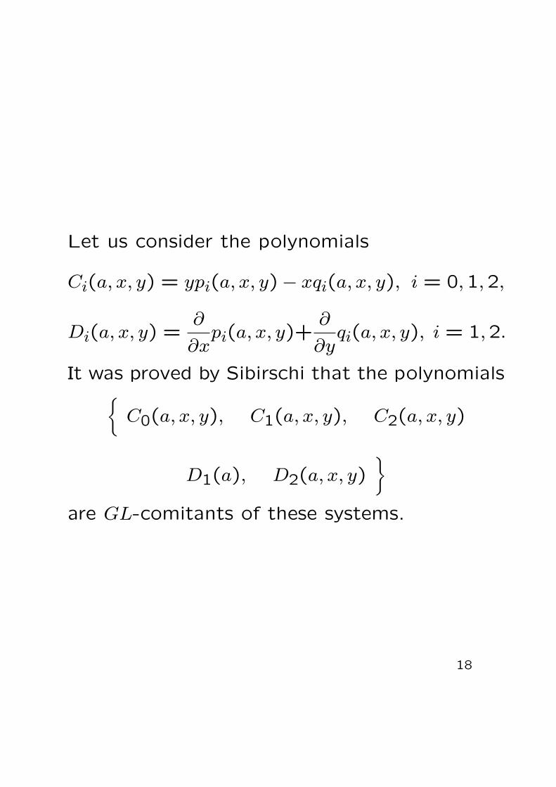
Let us consider the polynomials

Ci(a, x, y) = ypi(a, x, y)− xqi(a, x, y), i = 0,1,2,

Di(a, x, y) =∂

∂xpi(a, x, y)+

∂

∂yqi(a, x, y), i = 1,2.

It was proved by Sibirschi that the polynomials{C0(a, x, y), C1(a, x, y), C2(a, x, y)

D1(a), D2(a, x, y)}

are GL-comitants of these systems.

18

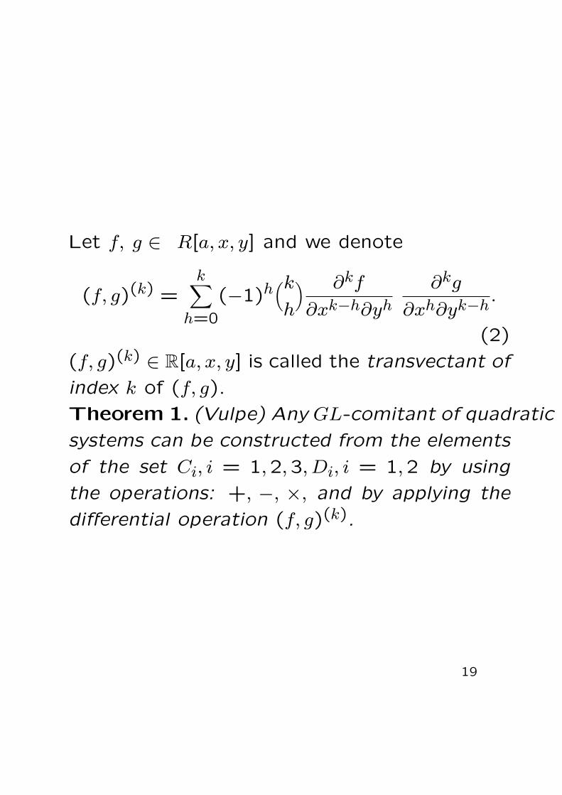
Let f, g ∈ R[a, x, y] and we denote

(f, g)(k) =k∑

h=0

(−1)h(kh

) ∂kf

∂xk−h∂yh∂kg

∂xh∂yk−h.

(2)

(f, g)(k) ∈ R[a, x, y] is called the transvectant of

index k of (f, g).

Theorem 1. (Vulpe) Any GL-comitant of quadratic

systems can be constructed from the elements

of the set Ci, i = 1,2,3, Di, i = 1,2 by using

the operations: +, −, ×, and by applying the

differential operation (f, g)(k).

19

Consider the differential operator

L = x · L2 − y · L1

acting on R[a, x, y] where

L1 = 2a00∂

∂a10+a10

∂

∂a20+

1

2a01

∂

∂a11+2b00

∂

∂b10+

b10∂

∂b20+

1

2b01

∂

∂b11,

L2 = 2a00∂

∂a01+a01

∂

∂a02+

1

2a10

∂

∂a11+2b00

∂

∂b01+

b01∂

∂b02+

1

2b10

∂

∂b11.

20

Using this operator and the affine invariant

µ0 = Res x

(p2(a, x, y), q2(a, x, y)

)/y4 we construct

the following polynomials µi(a, x, y) = 1i!L

(i)(µ0),

i = 1, ..,4 where L(i)(µ0) = L(L(i−1)(µ0)).

The other invariants and comitants of differ-

ential equations used for proving our main re-

sults are obtained by using these operations

and following the theory of algebraic invariants

of polynomial differential systems, developed

by Sibirsky and his disciples.

21

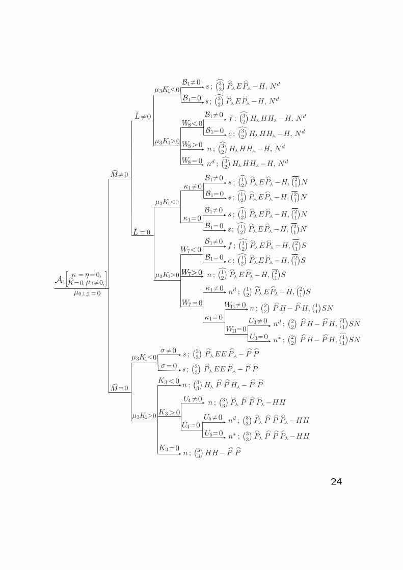
Main Theorem. (A) The configurations of

singularities, finite and infinite, of all quadratic

vector fields with a single finite singularity which

is simple (the total multiplicity of finite singu-

larities is mf = 1) are classified in the following

Diagram according to the geometric equiva-

lence relation. We have 52 geometrically dis-

tinct global configurations of singularities.

(B) Necessary and sufficient conditions for each

one of the 52 different equivalence classes can

be assembled from these diagram in terms of

25 invariant polynomials with respect to the

action of the affine group and time rescaling.

(C) The Diagram actually contains the global

bifurcation diagram in the 12-dimensional space

of parameters, of the global configurations of

singularities, finite and infinite, of this family

of quadratic differential systems.

22

23

24

The computation of polynomial invariants is

done using symbolic calculations.

This bifurcation diagram is expressed in terms

of polynomial invariants. The results can there-

fore be applied to any family of quadratic

systems, given in any normal form.

This diagram gives us also an algorithm for

computing the global configurations of sin-

gularities for any quadratic system given in

any possible normal form. We only need to

compute the indicated polynomials by follow-

ing step by step the Diagram.

========================

25

Here are some definitions of concepts used inthis work and some notations.In a classification we have two objects: a setX and an equivalence relation on X.

In this work X is the set of all global config-urations of singularities of systems in QS andthe equivalence relation on X is the geometric

equivalence relation which is finer than thetopological equivalence relation.

The topological equivalence relation does notdistinguish between foci and nodes, or betweenfoci of different orders.

The geometric equivalence relation distin-guishes between foci and nodes, between thestrong and weak foci, between strong and weaksaddles, between foci of different orders, be-tween saddles of different orders, between inte-grable saddles and weak saddles of positive or-ders, and between the different kinds of nodes.

26

Such distinctions are important in the produc-

tion of limit cycles. Indeed, for example the

maximum number of limit cycles which can be

produced close to the weak foci in perturba-

tions depends on the orders of the foci.

Topological versus geometrical

equivalence relations:

Two singularities are topologically equiva-

lent if they possess neighborhoods N1 and N2

for which there is a homeomorphism ϕ : N1 →N2 which carries oriented phase curves in N1

to oriented phase curves in N2 preserving the

orientation.

The notion of geometric equivalence rela-

tion is completely defined in terms of an alge-

braic nature.

27

Algebraic information may not be significant

for the local (topological) phase portrait around

a singularity. For example, topologically there

is no distinction between a focus and a node

or between a weak and a strong focus. But

algebraic information plays a fundamental role

in the study of perturbations of systems pos-

sessing such singularities.

28

We use the following terminology for singular-ities:

We call elemental a singular point with itsboth eigenvalues not zero;

We call semi–elemental a singular pointwith exactly one of its eigenvalues equal tozero;

We call nilpotent a singular point withboth its eigenvalues zero but with its Ja-cobian matrix at that point not identicallyzero;

We call intricate a singular point with itsJacobian matrix identically zero.

In the literature, intricate singularities are usu-ally called linearly zero.

29

Two singularities p1 and p2 of two polynomial

vector fields are locally geometrically equiv-

alent if and only if they are topologically equiv-

alent, they have the same multiplicity and one

of the following conditions is satisfied:

• p1 and p2 are order equivalent foci (or sad-

dles).

(Two foci (or saddles) are order equiva-

lent if their corresponding orders coincide);

• p1 and p2 are tangent equivalent simple

nodes

Two simple finite nodes, with the respec-

tive eigenvalues λ1, λ2 and σ1, σ2, are tan-

gent equivalent if and only if they sat-

isfy one of the following three conditions:

a) (λ1 − λ2)(σ1 − σ2) = 0; b) λ1 − λ2 =

0 = σ1 − σ2 and both linearization matri-

ces at the two singularities are diagonal; c)

30

λ1−λ2 = 0 = σ1−σ2 and the corresponding

linearization matrices are not diagonal.);

• p1 and p2 are both centers;

• p1 and p2 are both semi–elemental singu-

larities;

• p1 and p2 are blow–up equivalent nilpotent

or intricate singularities.

We say that two infinite simple nodes P1 and

P2 are tangent equivalent if and only if their

corresponding singularities on the sphere are

tangent equivalent and in addition, in case they

are generic nodes, we have (|λ1| − |λ2|)(|σ1| −|σ2|) > 0 where λ1 and σ1 are the eigenvalues of

the eigenvectors tangent to the line at infinity.

Multiplicity of singularities

Roughly speaking a singular point p of an an-alytic differential system χ is a multiple sin-gularity of multiplicity m if p generates m

singularities, as close to p as we wish, underanalytic perturbations of this system and m isthe maximal such number.In polynomial differential systems of fixed de-gree n we have several possibilities for obtain-ing multiple singularities. i) A finite singularpoint splits into several finite singularities inn-degree polynomial perturbations. ii) An in-finite singular point splits into some finite andsome infinite singularities in n-degree polyno-mial perturbations. iii) An infinite singularitysplits only in infinite singular points of the sys-tems in n-degree perturbations.To all these cases we can give a precise math-ematical meaning using the notion of intersec-tion multiplicity at a point p of two algebraiccurves based on work of D.S (1997), and D.Sand Pal (2001).

31

We denote the finite singularities with lower

case letters and the infinite ones with capital

letters placing first the finite ones, then the in-

finite ones, separating them by a semicolon‘;’.

Elemental points: We use the letters ‘s’,‘S’

for “saddles”; ‘n’, ‘N ’ for “nodes”; ‘f ’ for

“foci”; ‘c’ for “centers” and c⃝ (respectively

c⃝) for complex finite (respectively infinite) sin-

gularities. We distinguish the finite nodes as

follows:

• ‘n’ for a node with two distinct eigenvalues

(generic node);

• ‘nd’ (a one–direction node) for a node with

two identical eigenvalues whose Jacobian

matrix is not diagonal;

32

• ‘n∗’ (a star–node) for a node with two iden-

tical eigenvalues whose Jacobian matrix is

diagonal.

Moreover, in the case of an elemental infinite

generic node, we want to distinguish whether

the eigenvalue associated to the eigenvector

directed towards the affine plane is, in absolute

value, greater or lower than the eigenvalue as-

sociated to the eigenvector tangent to the line

at infinity. We will denote them as ‘N∞’ and

‘Nf ’ respectively.

When the trace of the Jacobian matrix of ele-

mental saddle and focus is zero, in the quadratic

case, one may have up to 3 finite orders. We

denote them by ‘s(i)’ and ‘f(i)’ where i = 1,2,3

is the order. In addition we have the centers

which we denote by ‘c’ and saddles of infinite

order (integrable saddles) which we denote by

‘$’.

To define the notion of geometric configura-

tion of singularities we distinguish two cases:

Case 1) in which we have a finite number of

infinite singular points. Then we call configu-

ration of singularities, finite and infinite, the

set of all these singularities each endowed with

its own multiplicity together with their local

phase portraits endowed with additional ge-

ometric structure involving the concepts of

tangent, order and blow–up equivalences.

Let χ1 and χ2 be two polynomial vector fields

each having a finite number of singularities.

We say that χ1 and χ2 have geometric equiv-

alent configurations of singularities if and

only if we have a bijection ϑ carrying the sin-

gularities of χ1 to singularities of χ2 and for

every singularity p of χ1, ϑ(p) is geometrically

equivalent with p.

33

2) If the line at infinity Z = 0 is filled up with

singularities, in each one of the charts at infin-

ity X = 0 and Y = 0, the system is degenerate

and we need to do a rescaling of an appropriate

degree of the system, so that the degeneracy

be removed. The resulting systems have only a

finite number of singularities on the line Z = 0.

In case 2) We call configuration of singular-

ities, finite and infinite, the union of the set

of all points at infinity (they are all singulari-

ties) with the set of finite singularities, taking

care of singling out the singularities of the “re-

duced” system at infinity, taken together with

the local phase portraits of finite singularities

endowed with additional geometric structure

as above and of the infinite singularities of the

reduced system.

34