Applied Analytics and Predictive Modeling

Spring 2021

Lecture-5

Lydia Manikonda

manikl@rpi.edu

Some of the slides adapted from Intro to Data Mining Tan et al. 2nd edition

Today’s agenda

• Case Study-1

• Data Quality

Case Study-1

• Due: February 18th 2021, 11:59 pm ET via LMS

• Olympics dataset

• Different dynamics and insights about Olympics using this data

• 4 teams will present in-class

• Every team will submit a report (max 8 pages including visualizations)

Image source: Wikipedia

Data Quality

• Poor data quality negatively affects many data processing efforts

“The most important point is that poor data quality is an unfolding disaster.

• Poor data quality costs the typical company at least ten percent (10%) of revenue; twenty percent (20%) is probably a better estimate.”

Thomas C. Redman, DM Review, August 2004

• Data mining example: a classification model for detecting people who are loan risks is built using poor data• Some credit-worthy candidates are denied loans

• More loans are given to individuals that default

Data Quality …

• What kinds of data quality problems?

• How can we detect problems with the data?

• What can we do about these problems?

• Examples of data quality problems: • Noise and outliers

• Missing values

• Duplicate data

• Wrong data

Noise• For objects, noise is an extraneous object

• For attributes, noise refers to modification of original values• Examples: distortion of a person’s voice when talking on a poor phone and

“snow” on television screen

Two Sine Waves Two Sine Waves + Noise

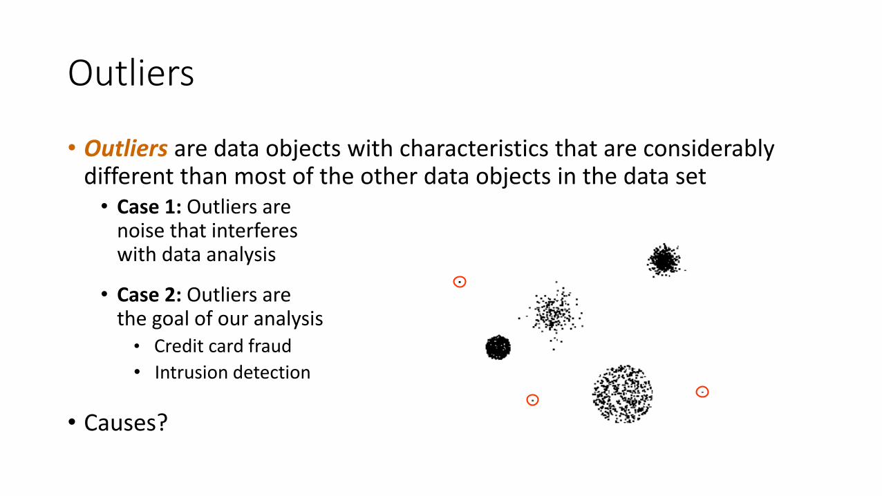
• Outliers are data objects with characteristics that are considerably different than most of the other data objects in the data set• Case 1: Outliers are

noise that interfereswith data analysis

• Case 2: Outliers are the goal of our analysis• Credit card fraud

• Intrusion detection

• Causes?

Outliers

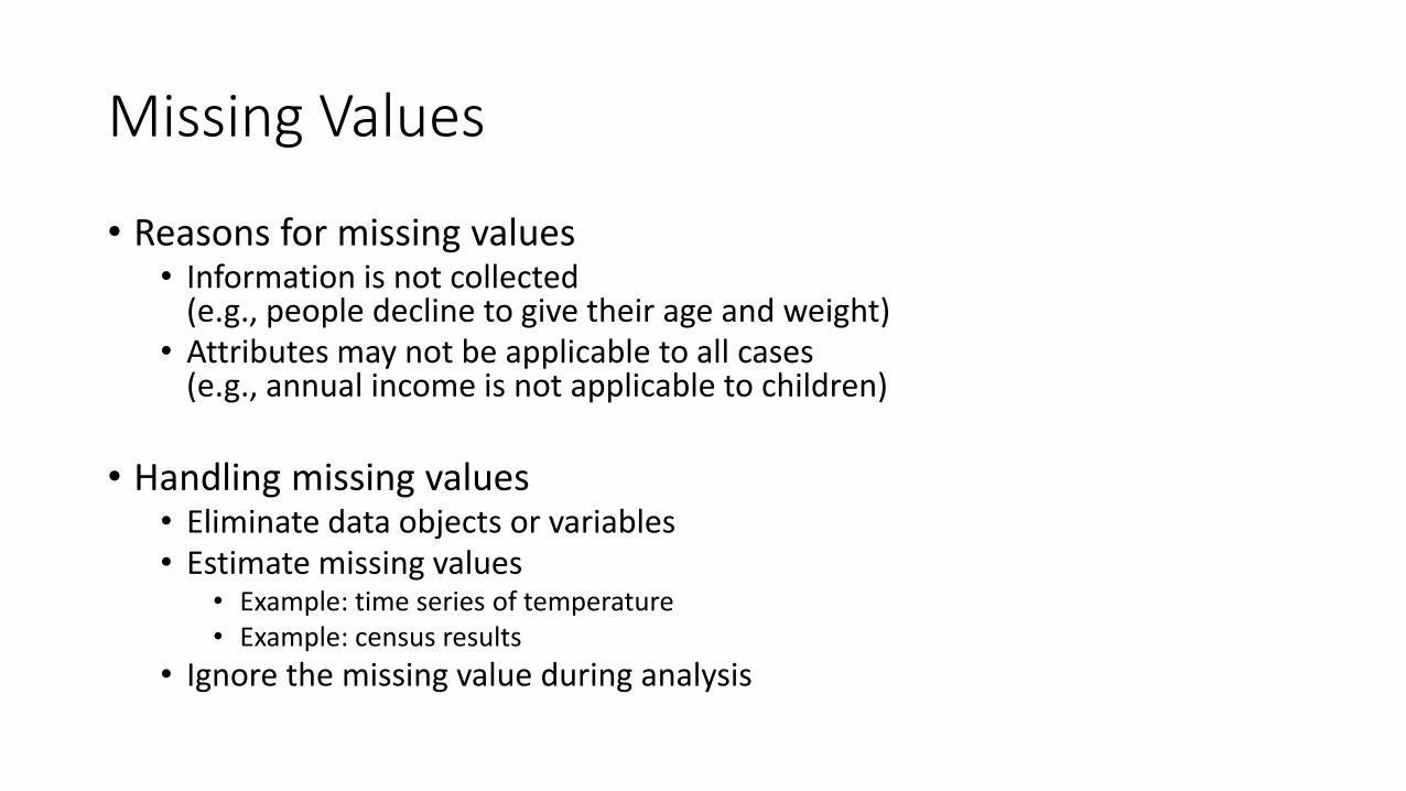
Missing Values

• Reasons for missing values• Information is not collected

(e.g., people decline to give their age and weight)• Attributes may not be applicable to all cases

(e.g., annual income is not applicable to children)

• Handling missing values• Eliminate data objects or variables• Estimate missing values

• Example: time series of temperature• Example: census results

• Ignore the missing value during analysis

Missing Values …

• Missing completely at random (MCAR)• Missingness of a value is independent of attributes• Fill in values based on the attribute• Analysis may be unbiased overall

• Missing at Random (MAR)• Missingness is related to other variables• Fill in values based on other values• Almost always produces a bias in the analysis

• Missing Not at Random (MNAR)• Missingness is related to unobserved measurements• Informative or non-ignorable missingness

• Not possible to know the situation from the data

Duplicate Data

• Data set may include data objects that are duplicates, or almost duplicates of one another• Major issue when merging data from heterogeneous sources

• Examples:• Same person with multiple email addresses

• Data cleaning• Process of dealing with duplicate data issues

• When should duplicate data not be removed?

Similarity and Dissimilarity Measures

• Similarity measure• Numerical measure of how alike two data objects are.

• Is higher when objects are more alike.

• Often falls in the range [0,1]

• Dissimilarity measure• Numerical measure of how different two data objects are

• Lower when objects are more alike

• Minimum dissimilarity is often 0

• Upper limit varies

• Proximity refers to a similarity or dissimilarity

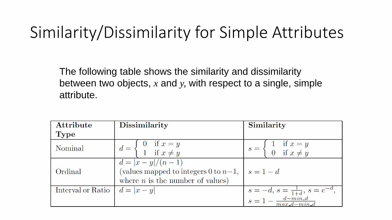
The following table shows the similarity and dissimilarity

between two objects, x and y, with respect to a single, simple

attribute.

Similarity/Dissimilarity for Simple Attributes

• Euclidean Distance

where n is the number of dimensions (attributes) and xk and yk are, respectively, the kth attributes (components) or data objects x and y.

• Standardization is necessary, if scales differ.

Euclidean Distance

0

1

2

3

0 1 2 3 4 5 6

p1

p2

p3 p4

point x y

p1 0 2

p2 2 0

p3 3 1

p4 5 1

Distance Matrix

p1 p2 p3 p4

p1 0 2.828 3.162 5.099

p2 2.828 0 1.414 3.162

p3 3.162 1.414 0 2

p4 5.099 3.162 2 0

Euclidean Distance

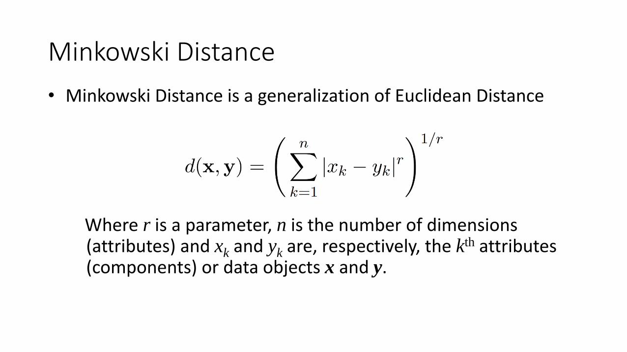
• Minkowski Distance is a generalization of Euclidean Distance

Where r is a parameter, n is the number of dimensions (attributes) and xk and yk are, respectively, the kth attributes (components) or data objects x and y.

Minkowski Distance

• r = 1. City block (Manhattan, taxicab, L1 norm) distance. • A common example of this is the Hamming distance, which is just the number

of bits that are different between two binary vectors

• r = 2. Euclidean distance

• r . “supremum” (Lmax norm, L norm) distance. • This is the maximum difference between any component of the vectors

• Do not confuse r with n, i.e., all these distances are defined for all numbers of dimensions.

Minkowski Distance: Examples

Minkowski Distance

Distance Matrix

point x y

p1 0 2

p2 2 0

p3 3 1

p4 5 1

L1 p1 p2 p3 p4

p1 0 4 4 6

p2 4 0 2 4

p3 4 2 0 2

p4 6 4 2 0

L2 p1 p2 p3 p4

p1 0 2.828 3.162 5.099

p2 2.828 0 1.414 3.162

p3 3.162 1.414 0 2

p4 5.099 3.162 2 0

L p1 p2 p3 p4

p1 0 2 3 5

p2 2 0 1 3

p3 3 1 0 2

p4 5 3 2 0

For red points, the Euclidean distance is 14.7, Mahalanobis distance is 6.

is the covariance matrix

𝐦𝐚𝐡𝐚𝐥𝐚𝐧𝐨𝐛𝐢𝐬 𝐱, 𝐲 = (𝐱 − 𝐲)𝑇 Ʃ−1(𝐱 − 𝐲)

Mahalanobis Distance

Mahalanobis DistanceCovariance

Matrix:

3.02.0

2.03.0

A: (0.5, 0.5)

B: (0, 1)

C: (1.5, 1.5)

Mahal(A,B) = 5

Mahal(A,C) = 4

B

A

C

• Distances, such as the Euclidean distance, have some well known properties.

1. d(x, y) 0 for all x and y and d(x, y) = 0 only if x = y. (Positive definiteness)

2. d(x, y) = d(y, x) for all x and y. (Symmetry)3. d(x, z) d(x, y) + d(y, z) for all points x, y, and z.

(Triangle Inequality)

where d(x, y) is the distance (dissimilarity) between points (data objects), xand y.

• A distance that satisfies these properties is a metric

Common Properties of a Distance

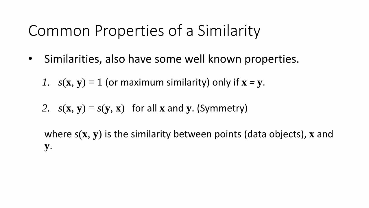
• Similarities, also have some well known properties.

1. s(x, y) = 1 (or maximum similarity) only if x = y.

2. s(x, y) = s(y, x) for all x and y. (Symmetry)

where s(x, y) is the similarity between points (data objects), x and y.

Common Properties of a Similarity

• Common situation is that objects, p and q, have only binary attributes

• Compute similarities using the following quantitiesf01 = the number of attributes where p was 0 and q was 1f10 = the number of attributes where p was 1 and q was 0f00 = the number of attributes where p was 0 and q was 0f11 = the number of attributes where p was 1 and q was 1

• Simple Matching and Jaccard Coefficients SMC = number of matches / number of attributes

= (f11 + f00) / (f01 + f10 + f11 + f00)

J = number of 11 matches / number of non-zero attributes= (f11) / (f01 + f10 + f11)

Similarity Between Binary Vectors

x = 1 0 0 0 0 0 0 0 0 0

y = 0 0 0 0 0 0 1 0 0 1

f01 = 2 (the number of attributes where p was 0 and q was 1)

f10 = 1 (the number of attributes where p was 1 and q was 0)

f00 = 7 (the number of attributes where p was 0 and q was 0)

f11 = 0 (the number of attributes where p was 1 and q was 1)

SMC = (f11 + f00) / (f01 + f10 + f11 + f00)

= (0+7) / (2+1+0+7) = 0.7

J = (f11) / (f01 + f10 + f11) = 0 / (2 + 1 + 0) = 0

SMC versus Jaccard: Example

• If d1 and d2 are two document vectors, thencos( d1, d2 ) = <d1,d2> / ||d1|| ||d2|| ,

where <d1,d2> indicates inner product or vector dot product of vectors, d1 and d2,

and || d || is the length of vector d.

• Example:

d1 = 3 2 0 5 0 0 0 2 0 0

d2 = 1 0 0 0 0 0 0 1 0 2<d1, d2> = 3*1 + 2*0 + 0*0 + 5*0 + 0*0 + 0*0 + 0*0 + 2*1 + 0*0 + 0*2 = 5

| d1 || = (3*3+2*2+0*0+5*5+0*0+0*0+0*0+2*2+0*0+0*0)0.5 = (42) 0.5 = 6.481

|| d2 || = (1*1+0*0+0*0+0*0+0*0+0*0+0*0+1*1+0*0+2*2) 0.5 = (6) 0.5 = 2.449

cos(d1, d2 ) = 0.3150

Cosine Similarity

Correlation measures the linear relationship between objects

Scatter plots

showing the

similarity from

–1 to 1.

Visually Evaluating Correlation

Information Based Measures

• Information theory is a well-developed and fundamental disciple with broad applications

• Some similarity measures are based on information theory • Mutual information in various versions

• Maximal Information Coefficient (MIC) and related measures

• General and can handle non-linear relationships

• Can be complicated and time intensive to compute

Information and Probability

• Information relates to possible outcomes of an event • transmission of a message, flip of a coin, or measurement of a piece of data

• The more certain an outcome, the less information that it contains and vice-versa• For example, if a coin has two heads, then an outcome of heads provides no

information

• More quantitatively, the information is related the probability of an outcome• The smaller the probability of an outcome, the more information it provides and vice-

versa

• Entropy is the commonly used measure

Entropy

• For • a variable (event), X, • with n possible values (outcomes), x1, x2 …, xn

• each outcome having probability, p1, p2 …, pn

• the entropy of X , H(X), is given by

𝐻 𝑋 = −

𝑖=1

𝑛

𝑝𝑖log2 𝑝𝑖

• Entropy is between 0 and log2n and is measured in bits• Thus, entropy is a measure of how many bits it takes to represent an observation of

X on average

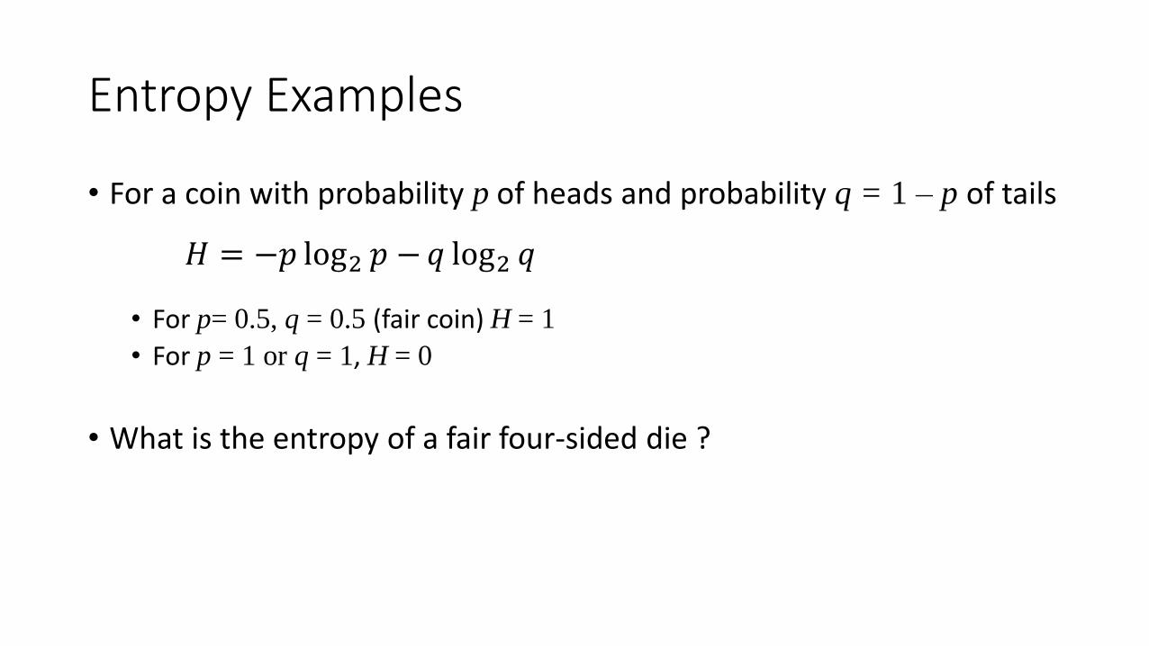
Entropy Examples

• For a coin with probability p of heads and probability q = 1 – p of tails

𝐻 = −𝑝 log2 𝑝 −𝑞 log2 𝑞

• For p= 0.5, q = 0.5 (fair coin) H = 1

• For p = 1 or q = 1, H = 0

• What is the entropy of a fair four-sided die ?

Entropy for Sample Data: Example

Hair Color Count p -plog2p

Black 75 0.75 0.3113

Brown 15 0.15 0.4105

Blond 5 0.05 0.2161

Red 0 0.00 0

Other 5 0.05 0.2161

Total 100 1.0 1.1540

Entropy for Sample Data

• Suppose we have • a number of observations (m) of some attribute, X, e.g., the gpa (assuming

rounded values) of students in the class, • where there are n different possible values• And the number of observation in the ith category is mi

• Then, for this sample

𝐻 𝑋 = −

𝑖=1

𝑛𝑚𝑖

𝑚log2

𝑚𝑖

𝑚

• For continuous data, the calculation is harder

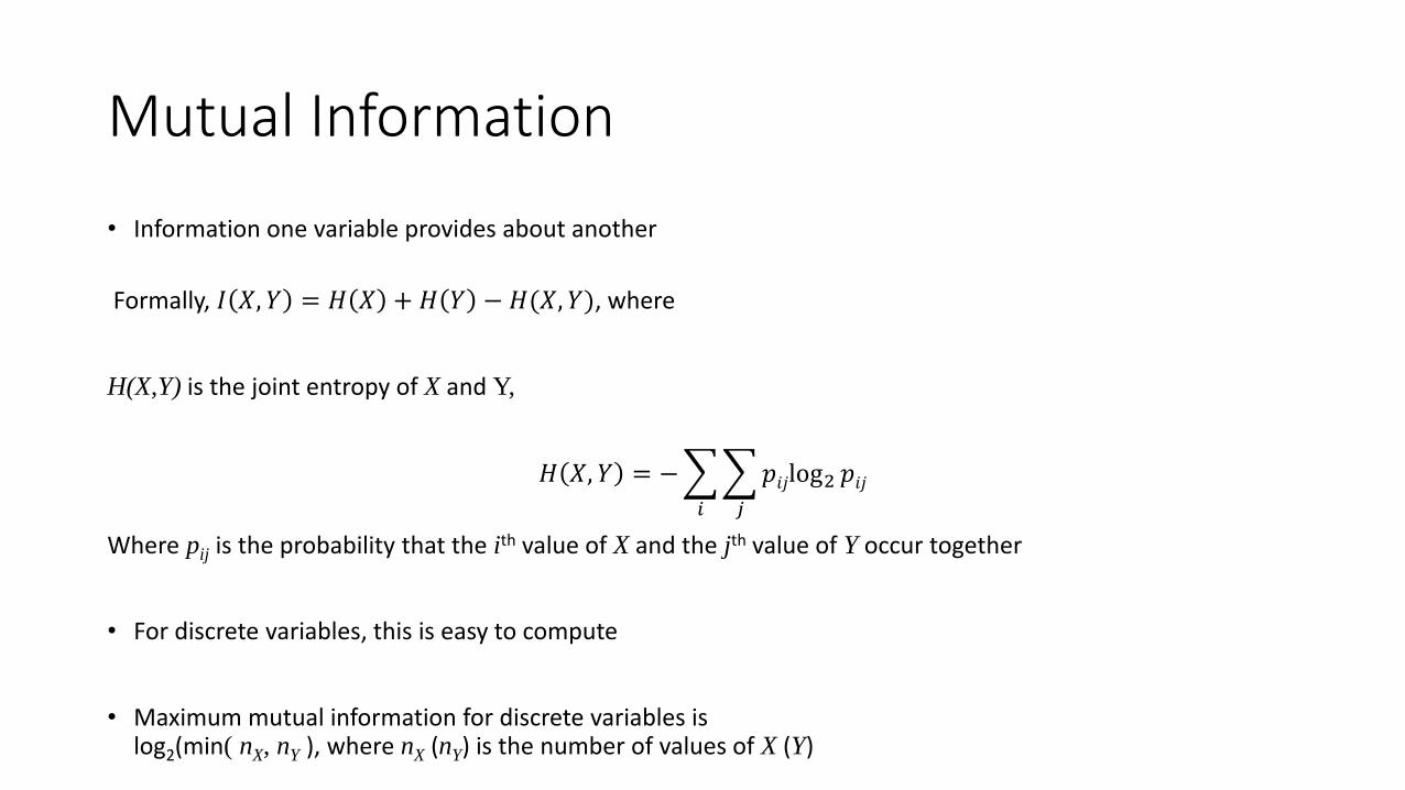
Mutual Information

• Information one variable provides about another

Formally, 𝐼 𝑋, 𝑌 = 𝐻 𝑋 + 𝐻 𝑌 − 𝐻(𝑋, 𝑌), where

H(X,Y) is the joint entropy of X and Y,

𝐻 𝑋, 𝑌 = −

𝑖

𝑗

𝑝𝑖𝑗log2 𝑝𝑖𝑗

Where pij is the probability that the ith value of X and the jth value of Y occur together

• For discrete variables, this is easy to compute

• Maximum mutual information for discrete variables is log2(min( nX, nY ), where nX (nY) is the number of values of X (Y)

Mutual Information ExampleStudent Status

Count p -plog2p

Undergrad 45 0.45 0.5184

Grad 55 0.55 0.4744

Total 100 1.00 0.9928

Grade Count p -plog2p

A 35 0.35 0.5301

B 50 0.50 0.5000

C 15 0.15 0.4105

Total 100 1.00 1.4406

Student Status

Grade Count p -plog2p

Undergrad A 5 0.05 0.2161

Undergrad B 30 0.30 0.5211

Undergrad C 10 0.10 0.3322

Grad A 30 0.30 0.5211

Grad B 20 0.20 0.4644

Grad C 5 0.05 0.2161

Total 100 1.00 2.2710

Mutual information of Student Status and Grade = 0.9928 + 1.4406 - 2.2710 = 0.1624

Density

• Measures the degree to which data objects are close to each other in a specified area

• The notion of density is closely related to that of proximity

• Concept of density is typically used for clustering and anomaly detection

• Examples:• Euclidean density

• Euclidean density = number of points per unit volume

• Probability density• Estimate what the distribution of the data looks like

• Graph-based density• Connectivity

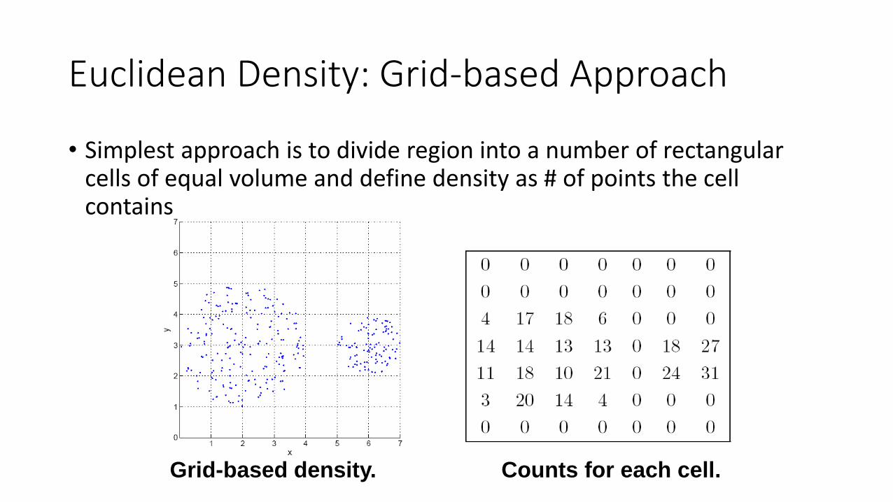
• Simplest approach is to divide region into a number of rectangular cells of equal volume and define density as # of points the cell contains

Grid-based density. Counts for each cell.

Euclidean Density: Grid-based Approach

Euclidean Density: Center-Based

• Euclidean density is the number of points within a specified radius of the point

Illustration of center-based density.