Applied Demography In Action: A Case Study of … · posed to applied demographers by clients and users in the 21st century. As such, budding applied demographers, especially those

Canadian Studies in Population, 2008, Vol. 35.1, pp. 133-158

CSP 2008, 35.1: 133-158 133

Applied Demography In Action:

A Case Study of “Population Identification.” *

David A. Swanson

Department of Sociology University of California Riverside Riverside, California USA 92521 [email protected]

Abstract

This case study deals with a problem quite different than the typical one facing most applied demographers. It involves the identification of a “population” using a set of criteria established by a regulatory agency. Specifically, criteria established by the US Nuclear Regulatory Commission for purposes of Site Characterization of the High Level Nuclear Waste Repository proposed for Yucca Mountain, Nevada. Consistent with other recent studies, this one suggests that a wide range of skills may be needed in dealing with problems posed to applied demographers by clients and users in the 21st century. As such, budding applied demographers, especially those nearing completion of their graduate studies, should consider adopting a set of skills beyond traditional demography. Key Words: Applied demography, population criteria

David A Swanson

CSP 2008, 35.1: 133-158

134

Résumé Cette étude de cas se centre sur un problème très différent des problèmes typiques qui confrontent les démographes en démographie appliquée. Ce cas-ci a pour sujet comment identifier une « population » en suivant un ensemble de critères établis par un organisme de régulation. Plus spécifiquement, des critères établis par le US Nuclear Regulatory Commission pour établir la caractérisation de site pour le Dépôt de déchets nucléaires de haute activité proposé à Yucca Mountain, au Nevada. En accord avec d’autres études récentes, la présente suggère qu’une grande étendue de compétences pourrait se prouver utiles aux démographes en démographie appliquée pour faire face aux problèmes présentés par les clients et les utilisateurs du XXIème siècle. À ce titre, les démographes en démographie appliquée débutants, et spécialement ceux qui tirent à la fin de leurs cycles supérieurs, devraient considérer se munir de compétences dont l’étendue dépasse la démographie appliquée traditionnelle. Mots-clés : Démographie appliquée, critères de population

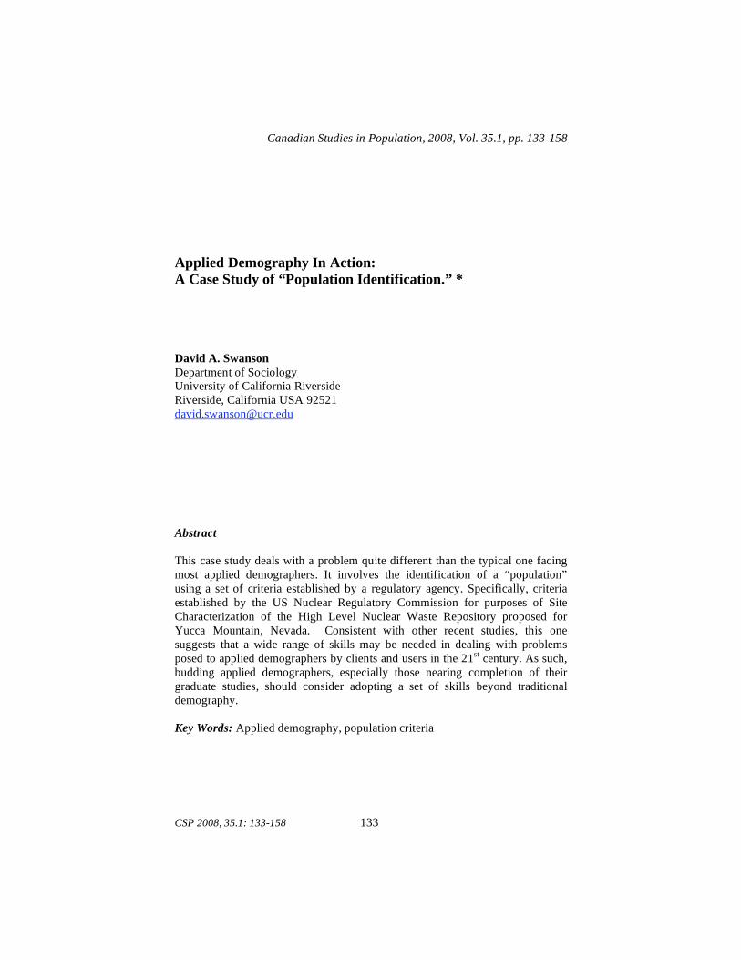
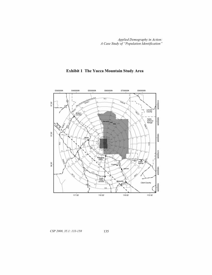
Introduction The research reported here was used to support the Biosphere component of the Total System Performance Assessment/Viability Assessment (TSPA/VA) for the high level nuclear waste repository proposed for Yucca Mountain, Nevada, which is located approximately 100 miles north of Las Vegas (U.S. DOE 1998). The research was used to determine if Yucca Mountain, Nevada was a suitable site for a spent nuclear fuel and high-level radioactive waste repository. This determination was positive: the Secretary of Energy recommended Yucca Mountain to the President as the repository site for highly radioactive materials and the President recommended the site to Congress. Exhibit 1 shows the general area around the site.

A key issue in determining if the Yucca Mountain site was suitable for the high level nuclear waste repository, was the identification of the “critical group,” an empirically-based population deemed to be at highest risk to the repository, with risk being related to exposure to the ingestion of radionuclides at levels dangerous to humans. The critical group was a crucial element in two areas: (1) deciding if the repository should go forward and: the design of man-made barriers for the repository. In identifying the critical group, two sets of “risk”

Applied Demography in Action: A Case Study of “Population Identification”

CSP 2008, 35.1: 133-158

135

Exhibit 1 The Yucca Mountain Study Area

David A Swanson

CSP 2008, 35.1: 133-158

136

parameters were generated: (1) a reasonable, conservative set; and (2) a high bounding set. These provided a set of parameters that are in the case of the first set, consistent with requirements for the critical group promulgated by the National Academy of Sciences as implemented in 10 CFR 63 (64 FR 8640) proposed by the Nuclear Regulatory Commission, and in the case of the second set, with an extremely conservative approach. The critical group and its risk parameters represent a conceptual model that was referenced as inputs to the process of generating “Biosphere Dose Conversion Factors” (BDCFs), which used the GENII-S computer code (SNL 1993).

Data

Parameters

The identification of a critical group and its characteristics relied on a 1997 Food Consumption Survey of the communities within the 50 mile centered on Yucca Mountain, Nevada (U.S. DOE 1997). The survey data were used primarily to determine the consumption levels for locally-produced food and tap water needed for ingestion exposure pathways. They also were used to develop a profile of the average member of the critical group for use in assessing exposure pathways other than food and water consumption.

In the survey, dietary and lifestyle data were collected on adults residing within the 50-mile grid centered on Yucca Mountain (U.S. DOE 199). Included within this grid are the communities of Amargosa Valley, Beatty, Indian Springs, and Pahrump (U.S. DOE 1997). The survey was a stratified random sample consisting of 1,079 respondents, of which 195 were in the Amargosa Valley. Criteria

In February 1999, the U.S. Nuclear Regulatory Commission (NRC) issued proposed “10 CFR 63,” which implemented the definition of a critical group and a reference biosphere in part 115 (64 FR 8640). Guidance issued by the Department of Energy (DOE) on the use of proposed 10 CFR 63 stated that individuals reasonably expected to receive the highest exposure under reasonable assumptions were to be used as the critical group (Dyer 1999). The NRC provides the following definition of the reference biosphere and the critical group in part 115 of proposed 10 CFR 63 (64 FRC 8640):


CSP 2008, 35.1: 133-158

137

a. Reference biosphere.

(1) Features, events, and processes that describe the reference biosphere shall be consistent with present knowledge of the conditions in the region surrounding the Yucca Mountain site. (2) Biosphere pathways shall be consistent with arid or semi-arid conditions. (3) Climate evolution shall be consistent with the geologic record of natural climate change in the region surrounding the Yucca Mountain site. (4) Evolution of the geologic setting shall be consistent with present knowledge of natural processes.

b. Critical group. (1) The critical group shall reside within a farming community located approximately 20 km south from the underground facility (in the general location of U.S. Route 95 and Nevada Route 373, near Lathrop Wells, Nevada). (2) The behaviors and characteristics of the farming community shall be consistent with current conditions of the region surrounding the Yucca Mountain site. Changes over time in the behaviors and characteristics of the critical group including, but not necessarily limited to, land use, lifestyle, diet, human physiology, or metabolics; shall not be considered. (3) The critical group resides within a farming community consisting of approximately 100 individuals, and exhibits behaviors or characteristics that will result in the highest expected annual doses. (4) The behaviors and characteristics of the average member of the critical group shall be based on the mean value of the critical group's variability range. The mean value shall not be unduly biased based on the extreme habits of a few individuals. (5) The average member of the critical group shall be an adult. Metabolic and physiological considerations shall be consistent with present knowledge of adults.

David A Swanson

CSP 2008, 35.1: 133-158

138

Analysis Using survey data from the food consumption survey as the source of input and having defined the critical group, summary descriptive statistics were then derived on the consumption of locally produced food and tap water.

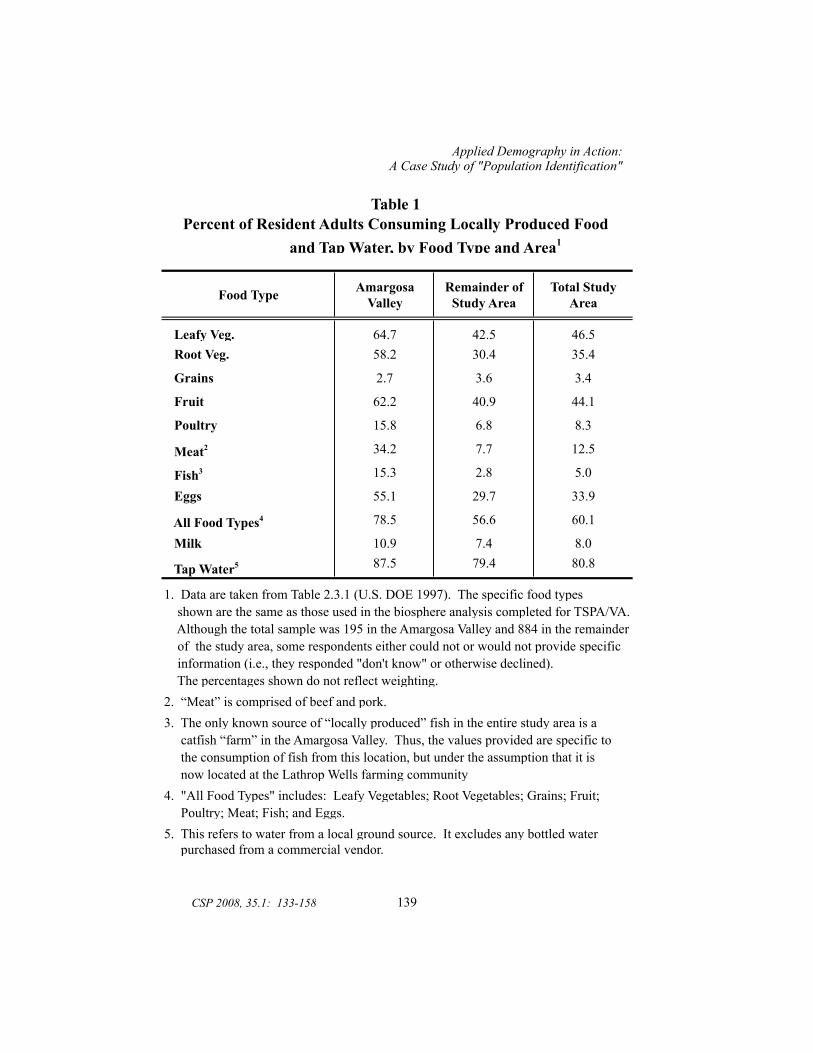
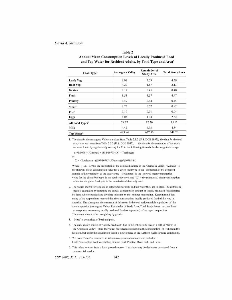
Among the communities in the vicinity of Yucca Mountain, Amargosa Valley is physically closest to the area selected by the NRC for the location of the critical group that could have been classified as a farming community based on production information (TRW 1998). The only source of food consumption data specific to the Amargosa Valley was the 1997 survey. Table 1 shows the percent of respondents consuming tap water and locally produced food, by type, for the Amargosa Valley and in the remainder of the study area. Specifically, Table 1 shows: (1) 79 of every 100 adults in the Amargosa Valley ate some type of locally produced food year prior to the survey compared to 57 out of every 100 in the remainder of the study area; (2) 88 out of every 100 adults in the Amargosa Valley reported consuming tap water compared to 79 out of 100 in the remainder of the study area; and (3) with the exception of grains, a higher percent of the adults in the Amargosa Valley consume locally produced food across all types than found in the remainder of the study area. For purposes of this study, the operational definition of an adult was that of a person 18 years of age and over. Table 2 shows that the average total consumption of locally produced food was higher in the Amargosa Valley (28.37 kg annually per adult) than in the remainder of the study area (12.20 kg annually per adult). The consumption of tap water also was higher in the Amargosa Valley (684 liters annually per adult) than in the remainder of the study area (646 liters annually per adult). With the exception of grains and milk, adults in the Amargosa Valley, on average, consumed more locally produced food across all food types than found in the remainder of the study area for the 1997 survey.

Of the 195 cases representing Amargosa Valley respondents, one had so many missing values that it was deemed unsuitable for analysis. Of the 194 usable cases, 77 reported that they both consumed locally produced food during the year prior to the survey and had a food garden. These 77 cases were found to exhibit homogeneous behaviors and characteristics and, as such, were used to define a critical group consistent with Proposed 10 CFR 63.

Food Type Amargosa Valley

Remainder of Study Area

Total Study Area

Leafy Veg. 64.7 42.5 46.5 Root Veg. 58.2 30.4 35.4

Grains 2.7 3.6 3.4

Fruit 62.2 40.9 44.1

Poultry 15.8 6.8 8.3

Meat2 34.2 7.7 12.5

Fish3 15.3 2.8 5.0

Eggs 55.1 29.7 33.9

All Food Types4 78.5 56.6 60.1

Milk 10.9 7.4 8.0

Tap Water5 87.5 79.4 80.8

2. “Meat” is comprised of beef and pork.3. The only known source of “locally produced” fish in the entire study area is a

4. "All Food Types" includes: Leafy Vegetables; Root Vegetables; Grains; Fruit;

shown are the same as those used in the biosphere analysis completed for TSPA/VA. Although the total sample was 195 in the Amargosa Valley and 884 in the remainder of the study area, some respondents either could not or would not provide specific information (i.e., they responded "don't know" or otherwise declined). The percentages shown do not reflect weighting.

purchased from a commercial vendor.

Table 1 Percent of Resident Adults Consuming Locally Produced Food

and Tap Water, by Food Type and Area1

catfish “farm” in the Amargosa Valley. Thus, the values provided are specific to the consumption of fish from this location, but under the assumption that it is now located at the Lathrop Wells farming community

Poultry; Meat; Fish; and Eggs.5. This refers to water from a local ground source. It excludes any bottled water

1. Data are taken from Table 2.3.1 (U.S. DOE 1997). The specific food types

139

Applied Demography in Action:A Case Study of "Population Identification"

CSP 2008, 35.1: 133-158

David A Swanson

CSP 2008, 35.1: 133-158

140

The set of 77 cases was found by using the "filter" procedure in NCSS (Hintze 1995) to select from the survey respondent file those respondents who met the following three conditions: (1) located in the Amargosa Valley; (2) had a food garden last year; and (3) consumed locally produced food. Upon activating this filter, the NCSS procedure "Descriptive Tables" (Hintze 1995,) was used to collect summary statistics, including a count of the number of respondents satisfying the three conditions set in the filter. The procedure revealed that 77 respondents met the desired criteria. Once it was known that 77 respondents met the desired criteria, the NCSS "Sort" procedure (Hintze 1995) was used in two steps to assemble the 77 cases representing these respondents at the top of the file. This was done only while the master survey file was active, which means that the sorted cases were not made a permanent feature of the master file. In the first step, the sort feature was set so that only those 194 cases from the Amargosa Valley were found at the top of the file. When this was done, the remaining cases were deleted from the active file and the active file was saved as a new file. In the second step, the sort feature was applied to the active file by sorting on two variables simultaneously so that the 77 cases in question were represented at the top of the file: Presence of a garden; and consumed locally produced food. When this step was accomplished, the topmost 77 cases were kept by deleting the remaining 117 cases.

With the second step accomplished, the 77 cases remaining represented members of the hypothetical farming community located near Lathrop Wells. They formed a group that exhibited behaviors and habits that were expected to result in the highest expected doses. There are 28 male respondents and 49 female respondents in this set. As is reported in the documentation for the survey, males were under-represented in both the survey as a whole and each of its constituent communities (U.S. DOE 1997). This would not be important if males and females had the same daily intake of food, but this is not the case. Males consume on average different amounts than females (U.S. DOE 1997). It was known in advance of the survey that this disproportionate representation by gender was likely to occur and weights were developed to compensate for it (U.S. DOE 1997). The proportion of adult females in the Amargosa Valley was estimated to be .49 (U.S. DOE 1997) while the proportion of adult females in the sample is .615. That is, 120 of the 195 sample respondents were female while we expected that there should have been only 96 females, based on the proportion that represent of the adult population. Weighting is required so that the input parameters such as the mean reflect the proportion of females in the Amargosa Valley adult population, not the proportion in the sample. For the


CSP 2008, 35.1: 133-158

141

Amargosa Valley, the gender weights were already determined (U.S. DOE 1997): for a female it was 0.80; and for a male it was 1.32. That is, every 100 females comprise 80 females in the context of the weighted results for the Amargosa Valley while every 100 males comprise 132.

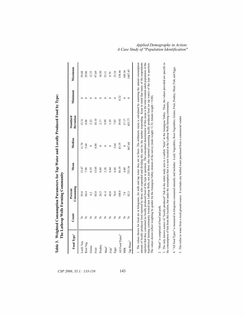
Males also were under-represented in the set of 77 respondents selected to live in the Lathrop Wells farming community. There were 28 males and 49 females in this set. Again we would expect females to represent about half of the Lathrop Wells farming community, but they represented about 64 percent. This suggested that the parameters for the critical group should be assembled from data weighted by gender (post-stratification). To achieve this end, the weights developed for the Amargosa Valley as a whole were applied to the set of 77 respondents selected to live in the Lathrop Wells farming community. That is, each male was weighted by a factor of 1.32 and each female by a factor of .80. This gender weighting scheme was deemed to be appropriate because the 77 respondents making up the hypothetical Lathrop Wells farming community were taken from a random sample of the Amargosa Valley population. This population is, recall, the one deemed to be at highest risk to exposure. Because there was neither a "random sample" nor a "population" associated with the hypothetical Lathrop Wells farming community, there is no other empirical basis on which a set of alternative gender-based weights could have been developed. While the weighting scheme selected for the Lathrop Wells had the advantage of being based on the gender distribution of the population of the Amargosa Valley, it also had a slight drawback: when the results are weighted, algebraically, there are 37 males and 39 females. That is, the weighted results sum to 76 rather than 77 respondents. This drawback was deemed acceptable in order to have weights based on a random sample of the "real" population deemed to be at highest risk, Amargosa Valley. The parameters for the consumption of locally produced food and tap water for this weighted set are shown in Table 3.

The survey data underlying the data presented in Table 3 were subject to error from a number of sources. However, tests done in regard to non-response bias as well as validity and reliability tests suggested that the survey data are valid and reliable and generally adequate for biosphere modeling purposes. Thus, the data in Table 3 as well as other data from the survey were found adequate for the task of developing both sets of parameters: (1) the reasonable, conservative estimates and their statistical distributions, which are in accordance with proposed 10 CFR 63; and (2) the high bounding values, which were, recall, designed to provide an extremely conservative set of parameters.

Food Type2 Amargosa Valley Remainder of Study Area Total Study Area

Leafy Veg. 8.01 3.59 4.39Root Veg. 4.20 1.67 2.13

Grains 0.17 0.45 0.40

Fruit 8.53 3.57 4.47

Poultry 0.49 0.44 0.45

Meat3 2.75 0.52 0.92

Fish4 0.19 0.01 0.04

Eggs 4.03 1.94 2.32

All Food Types5 28.37 12.20 15.12

Milk 4.42 4.93 4.84

Tap Water6 683.84 637.90 646.20

commercial vendor.

5. "All Food Types" is measured in kilograms consumed annually and includes: Leafy Vegetables; Root Vegetables; Grains; Fruit; Poultry; Meat; Fish; and Eggs.

6. This refers to water from a local ground source. It excludes any bottled water purchased from a

3. “Meat” is comprised of beef and pork.

4. The only known source of “locally produced” fish in the entire study area is a catfish “farm” in the Amargosa Valley. Thus, the values provided are specific to the consumption of fish from this location, but under the assumption that it is now located at the Lathrop Wells farming community.

area in question (Amargosa Valley, Remainder of Study Area, Total Study Area), not just those who reported consuming locally produced food (or tap water) of the type in question. The values shown reflect weighting by gender.

mean is calculated by summing the annual consumption amount of locally produced food reported by those who responded and dividing this sum by the number responding. Keep in mind that many of the respondents reported that they consumed no locally produced food of the type in question. The conceptual denominator of this mean is the total resident adult population of the

value for the given food type in the total study area; and "X" is the (unknown) mean consumption value for the given food type in the remainder of the study area.

2. The values shown for food are in kilograms; for milk and tap water they are in liters. The arithmetic

the (known) mean consumption value for a given food type in the proportion of the achieved sample in the remainder of the study area; "Totalmean" is the (known) mean consumption

Table 2Annual Mean Consumption Levels of Locally Produced Food

and Tap Water for Resident Adults, by Food Type and Area1

(195/1079)*(AVmean) + (884/1079)*(X) = Totalmean or X = (Totalmean - ((195/1079)*(AVmean)))*(1079/884)

Where: (195/1079) is the proportion of the achieved sample in the Amargosa Valley; "Avmean" is

1. The data for the Amargosa Valley are taken from Table 2.3.5 (U.S. DOE 1997); the data for the total study area are taken from Table 2.3.2 (U.S. DOE 1997); the data for the remainder of the study are were found by algebraically solving for X in the following formula for the weighted average.

David A. Swanson

142CSP 2008, 35.1: 133-158

Tabl

e 3.

Wei

ghte

d C

onsu

mpt

ion

Para

met

ers f

or T

ap W

ater

and

Loc

ally

Pro

duce

d Fo

od b

y Ty

pe:

T

he L

athr

op W

ells

Far

min

g C

omm

unity

Leaf

y Ve

g.76

95.0

15.4

711

.70

15.3

10

59.6

8R

oot V

eg.

7684

.47.

985.

688.

060

29.8

6

Gra

ins

764.

20.

390

2.22

012

.33

Frui

t76

85.0

15.0

58.

8818

.10

097

.69

Poul

try76

26.5

0.89

02.

170

10.5

0

Mea

t276

41.4

3.28

09.

990

53.1

1

Fish

376

40.8

0.44

01.

590

8.79

Eggs

7676

.06.

683.

647.

850

33.3

4

All

Food

Typ

es4

7610

0.0

50.1

943

.19

39.9

20.

3215

8.46

Milk

767.

84.

000

17.1

70

100.

36

Tap

Wat

er5

7692

.375

3.36

867.

6845

3.77

014

87.4

5

2. “

Mea

t” is

com

pris

ed o

f bee

f and

por

k.3.

The

only

know

nso

urce

of“l

ocal

lypr

oduc

ed”

fish

inth

een

tire

stud

yar

eais

aca

tfish

“far

m”

inth

eA

mar

gosa

Valle

y.Th

us,t

heva

lues

prov

ided

are

spec

ific

toth

e co

nsum

ptio

n of

fish

from

this

loca

tion,

but

und

er th

e as

sum

ptio

n th

at it

is n

ow lo

cate

d at

the

Lath

rop

Wel

ls fa

rmin

g co

mm

unity

.

1.Th

eva

lues

show

nfo

rfoo

dar

ein

kilo

gram

s;fo

rm

ilkan

dta

pw

ater

they

are

inlit

ers.

The

arith

met

icm

ean

isca

lcul

ated

bysu

mm

ing

the

annu

alco

nsum

ptio

nam

ount

oflo

cally

prod

uced

food

repo

rted

byth

ose

who

resp

onde

dan

ddi

vidi

ngth

issu

mby

the

num

berr

espo

ndin

g.K

eep

inm

ind

that

man

yof

the

resp

onde

nts

repo

rted

that

they

cons

umed

nolo

cally

prod

uced

food

ofth

ety

pein

ques

tion.

The

conc

eptu

alde

nom

inat

orof

this

mea

nis

the

tota

lres

iden

tadu

ltpo

pula

tion

ofth

ehy

poth

etic

alfa

rmin

gco

mm

unity

loca

ted

near

Lath

rop

Wel

ls,n

otju

stth

ose

who

repo

rted

cons

umin

glo

cally

prod

uced

food

(ort

apw

ater

)of

the

type

inqu

estio

n.Th

e va

lues

show

n re

flect

wei

ghtin

g by

gen

der f

or th

e Am

argo

sa V

alle

y st

ratu

m o

f the

surv

ey (m

ale

wei

ght =

1.32

; fem

ale

wei

ght =

0.8

0).

4. "

All

food

Typ

es"

is m

easu

red

in k

ilogr

ams c

onsu

med

ann

ually

and

incl

udes

: Le

afy

Vege

tabl

es; R

oot V

eget

able

s; G

rain

s; F

ruit;

Pou

ltry;

Mea

t; Fi

sh; a

nd E

ggs.

5. T

his r

efer

s to

wat

er fr

om a

loca

l gro

und

sour

ce.

It ex

clud

es a

ny b

ottle

d w

ater

pur

chas

ed fr

om a

com

mer

cial

ven

dor.

Food

Typ

e1C

ount

Max

imum

M

inim

umSt

anda

rd

Dev

iatio

n

M

edia

n

M

ean

Perc

ent

Con

sum

ing


143CSP 2008, 35.1: 133-158

David A Swanson

CSP 2008, 35.1: 133-158

144

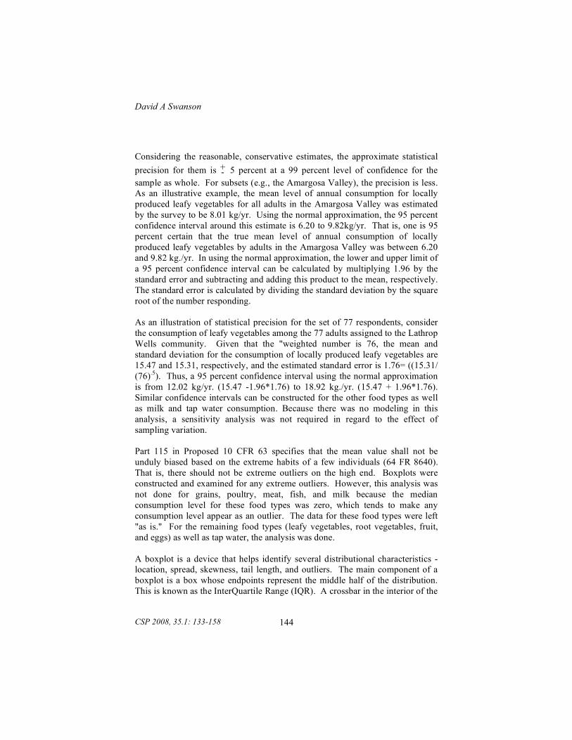
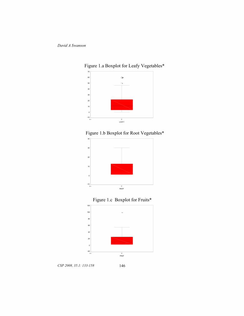
Considering the reasonable, conservative estimates, the approximate statistical precision for them is +- 5 percent at a 99 percent level of confidence for the sample as whole. For subsets (e.g., the Amargosa Valley), the precision is less. As an illustrative example, the mean level of annual consumption for locally produced leafy vegetables for all adults in the Amargosa Valley was estimated by the survey to be 8.01 kg/yr. Using the normal approximation, the 95 percent confidence interval around this estimate is 6.20 to 9.82kg/yr. That is, one is 95 percent certain that the true mean level of annual consumption of locally produced leafy vegetables by adults in the Amargosa Valley was between 6.20 and 9.82 kg./yr. In using the normal approximation, the lower and upper limit of a 95 percent confidence interval can be calculated by multiplying 1.96 by the standard error and subtracting and adding this product to the mean, respectively. The standard error is calculated by dividing the standard deviation by the square root of the number responding. As an illustration of statistical precision for the set of 77 respondents, consider the consumption of leafy vegetables among the 77 adults assigned to the Lathrop Wells community. Given that the "weighted number is 76, the mean and standard deviation for the consumption of locally produced leafy vegetables are 15.47 and 15.31, respectively, and the estimated standard error is 1.76= ((15.31/ (76).5). Thus, a 95 percent confidence interval using the normal approximation is from 12.02 kg/yr. (15.47 -1.96*1.76) to 18.92 kg./yr. (15.47 + 1.96*1.76). Similar confidence intervals can be constructed for the other food types as well as milk and tap water consumption. Because there was no modeling in this analysis, a sensitivity analysis was not required in regard to the effect of sampling variation. Part 115 in Proposed 10 CFR 63 specifies that the mean value shall not be unduly biased based on the extreme habits of a few individuals (64 FR 8640). That is, there should not be extreme outliers on the high end. Boxplots were constructed and examined for any extreme outliers. However, this analysis was not done for grains, poultry, meat, fish, and milk because the median consumption level for these food types was zero, which tends to make any consumption level appear as an outlier. The data for these food types were left "as is." For the remaining food types (leafy vegetables, root vegetables, fruit, and eggs) as well as tap water, the analysis was done. A boxplot is a device that helps identify several distributional characteristics - location, spread, skewness, tail length, and outliers. The main component of a boxplot is a box whose endpoints represent the middle half of the distribution. This is known as the InterQuartile Range (IQR). A crossbar in the interior of the


CSP 2008, 35.1: 133-158

145

box denotes the median and the tails are represented by a line drawn from each end of the box to the most remote point that is not an outlier. These points are known as upper and lower adjacent values, respectively. The upper adjacent value is the largest observation less than or equal to the 75th percentile plus 1.5 times IQR; the lower adjacent value is the smallest observation greater than or equal to the 25th percentile plus 1.5 times IQR (Hintze 1995).

The length of the box displays variability in the data. The relative position of the median in the box and the length and direction of the tails depict the distributional shape of the observations. A median closer to the lower end of the box with a long upper tail indicates a right-skewed distribution. Conversely, a median closer to the upper end of the box with a long lower tail suggests a left-skewed distribution. A median in the middle of the box with lower and upper tails of equal length is characteristic of a symmetrical distribution.

Keep in mind that the width of a boxplot has no substantive meaning. A given width is simply designed to provide a balance that is pleasing to the eye. This means that the tick marks on the horizontal axis have no substantive meaning and are simply an artifact of the NCSS boxplot procedure.

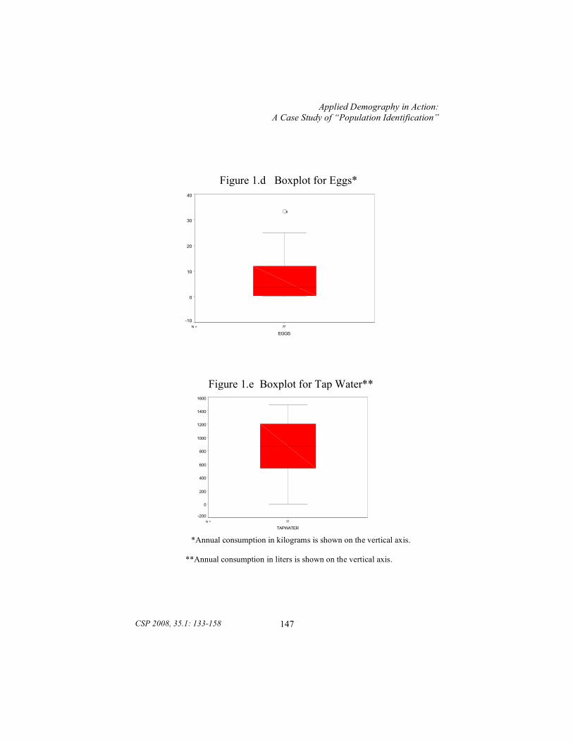
Values outside the upper and lower adjacent values are identified as outliers. There are two types of outliers, mild and severe (Hintze 1995). A mild outlier is one that is less than 3 IQRs from the nearest adjacent value; a severe outlier is 3 or more IQRs from the nearest adjacent value (Hintze 1995). The statistical package used to construct the boxplots (NCSS 6.0) has the capability to identify severe and mild outliers directly from a boxplot. That is, the package will perform all the calculations and the user need only specify that severe and mild outliers are represented by different symbols (Hintze 1995). For purposes of this analysis, a circle was selected to represent mild outliers and a square was selected to represent severe outliers. The boxplots for each of the variables of interest are shown below as figures 1a through 1e. In each part of the figure, the number shown on the vertical axis indicates average consumption per year. For food, this is given in kilograms, while for milk and tap water, it is given in liters. The boxplots show that the food consumption is right-skewed and truncated on the left at zero (nobody consumes a negative amount of locally produced food or tap water). This is supported by the finding that for each of the nine food types, the median is less than the mean, as shown in Table 3. In regard to the consumption of tap water, the distribution is not right-skewed.

David A Swanson

CSP 2008, 35.1: 133-158

146

Figure 1.a Boxplot for Leafy Vegetables*

77N =

LEAFY

70

60

50

40

30

20

10

0

-10

4

61413

Figure 1.b Boxplot for Root Vegetables*

77N =

ROOT

40

30

20

10

0

-10

Figure 1.c Boxplot for Fruits*

77N =

FRUIT

120

100

80

60

40

20

0

-20

1


CSP 2008, 35.1: 133-158

147

Figure 1.d Boxplot for Eggs*

77N =

EGGS

40

30

20

10

0

-10

8

Figure 1.e Boxplot for Tap Water**

77N =

TAPWATER

1600

1400

1200

1000

800

600

400

200

0

-200

*Annual consumption in kilograms is shown on the vertical axis. **Annual consumption in liters is shown on the vertical axis.

David A Swanson

CSP 2008, 35.1: 133-158

148

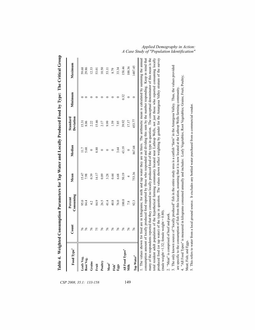
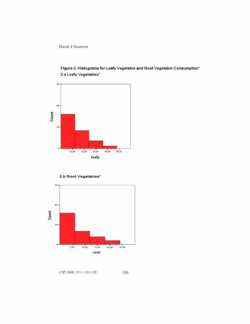
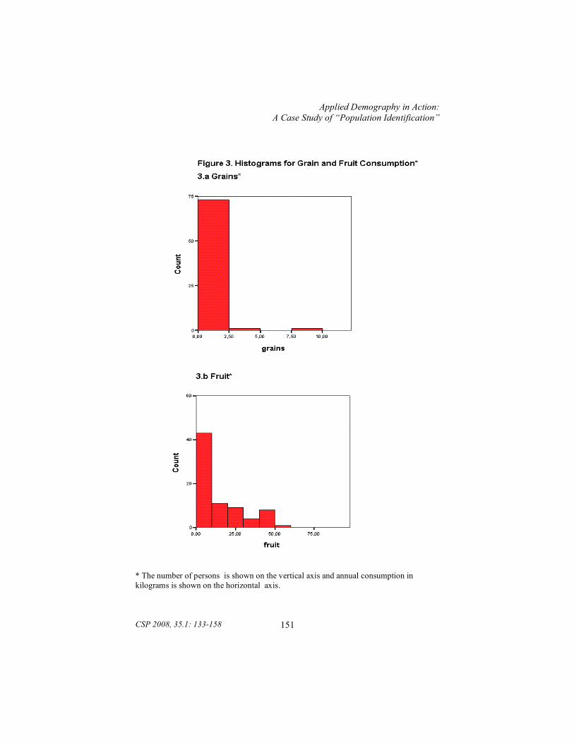
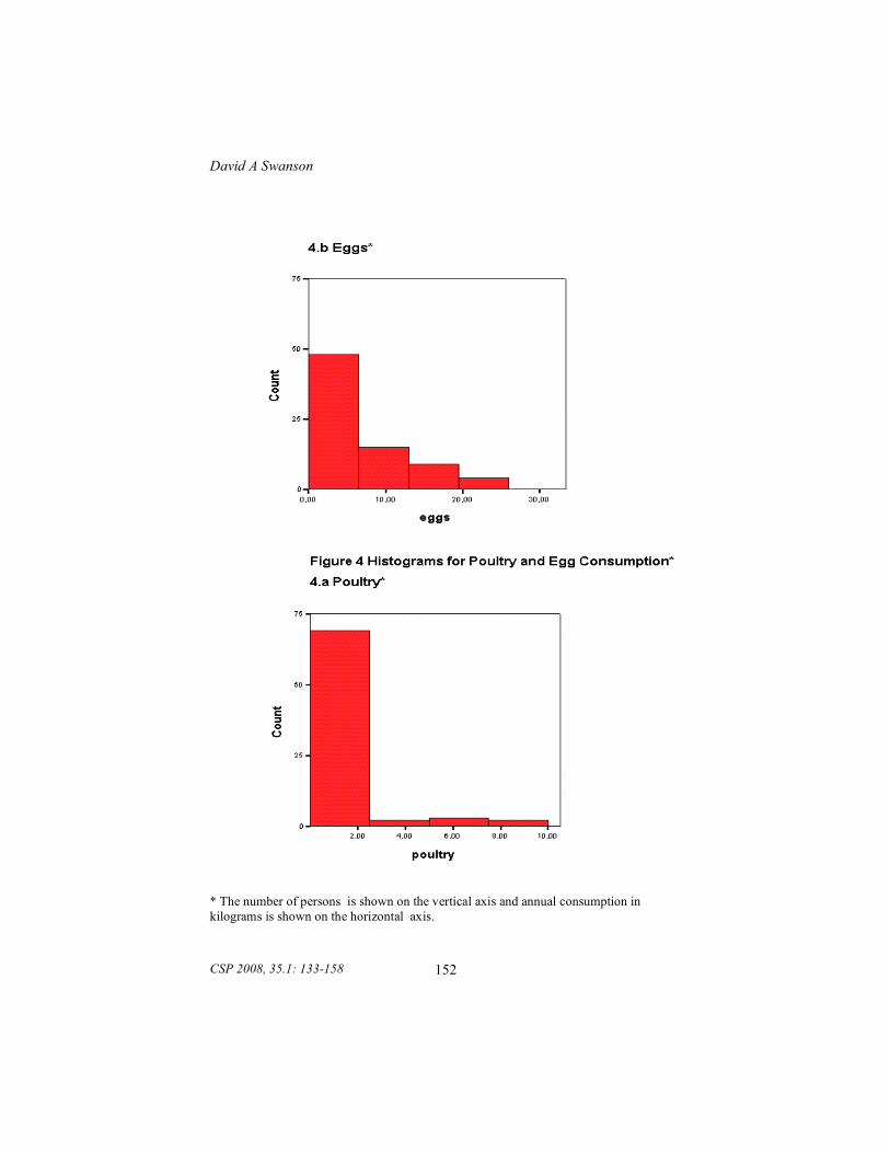
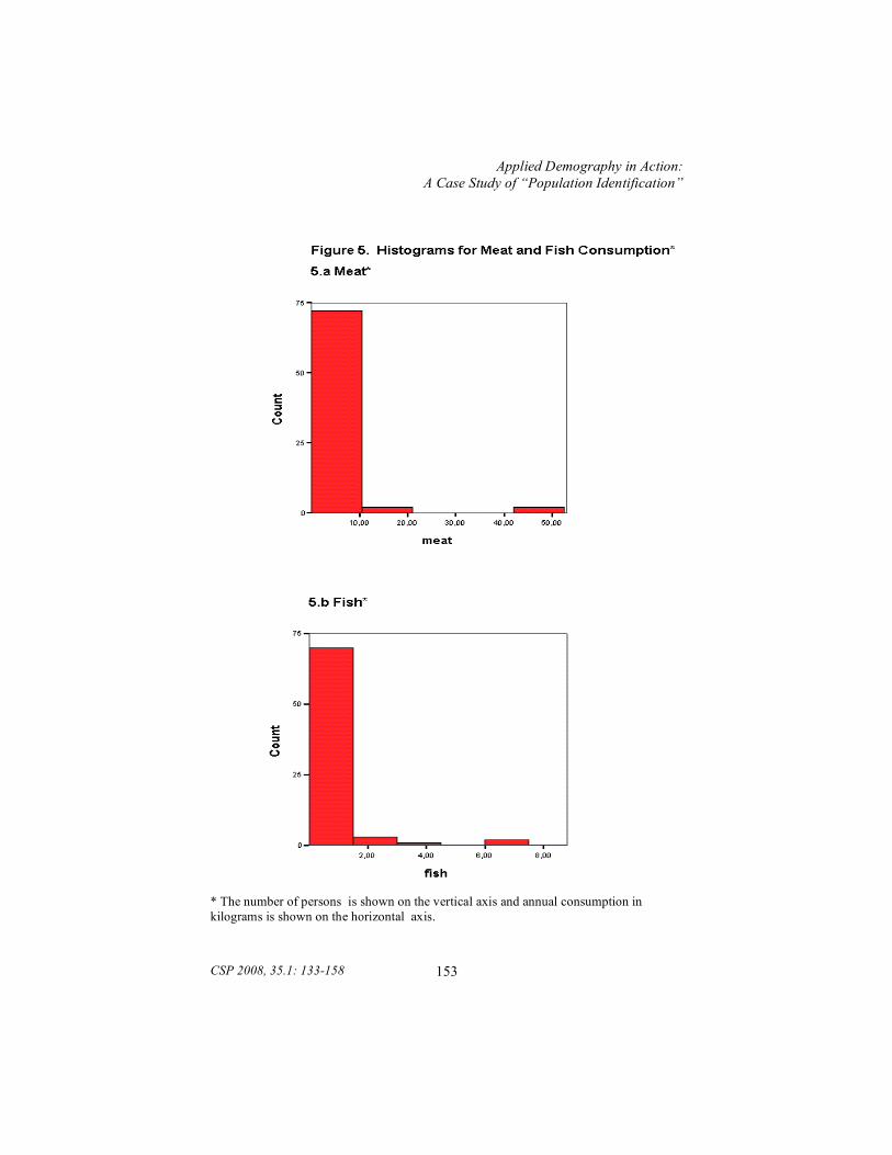
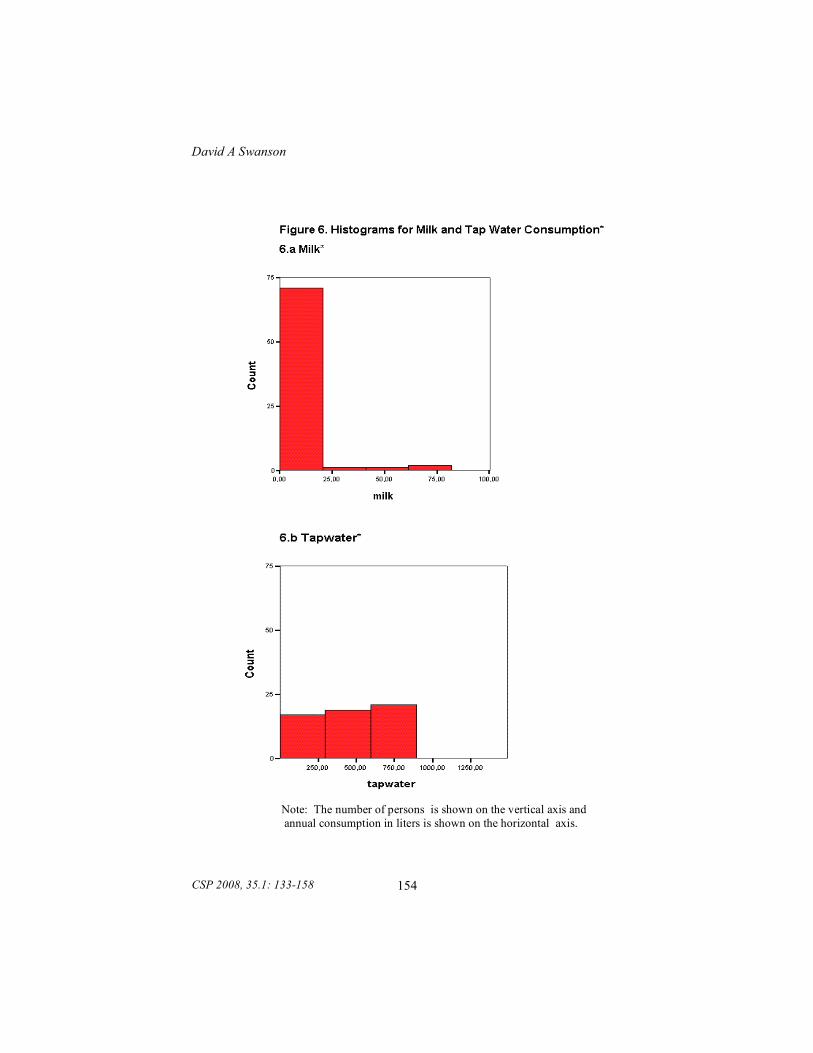
For two of the five variables in which the median is not zero, root vegetables (Figure 1b) and tap water (Figure 1e) there are no outliers identified. Thus, there are no extreme values. For the two of the remaining three, leafy vegetables (Figure 1a) and eggs (Figure 1d), each outlier is displayed as a circle, which means that they are not severe. However, for the third, fruit consumption (Figure 1c), there is a single outlier in the shape of a square, which means it is severe. This outlier is the maximum value for fruit consumption, 97.69, as shown in Table 3. Table 4 shows the parameters for the critical group located in the hypothetical framing community near Lathrop Wells, as found using the "outlier" analysis. With the exception of fruit consumption, the parameters shown are the same as those in Table 1. For fruit consumption, omitting the extreme value of 97.69 resulted in a change in the mean consumption level, from 15.05 to 14.17, in the maximum value, which fell to 53.01, and in the standard deviation, which decreased from 18.10 to 15.46. The maximum values shown in Table 4 were used for the second set of parameters, the bounding values. This set of maximum values was useful for this purpose because they were consistent with the reasonable, conservative parameters in that they provide bounding limits to the reasonable, conservative consumption levels. Histograms showing the distribution of consumption for each food type as well as milk and tap water are provided as Figures 2 through 7. The numbers on the vertical axis of each histogram show the number of respondents, while the numbers on the horizontal axis of each histogram show the level of consumption.

The graphs and data suggest that the consumption of locally produced food of all types was likely to follow a negative exponential distribution, while tap water was likely to follow a uniform distribution, although there are other distributions that could provide an adequate fit as well. It was known the software to be used to develop ingestion exposure estimates, “GENII-S,” accommodated a uniform distribution, but not a negative exponential distribution (SNL 1993). Of the distributions found in GENII-S, the log uniform appeared to be the most suitable substitute for the negative exponential. As a consequence, the log uniform distribution was recommended for use with all food types in terms of the reasonable, conservative set of estimated parameters.

Two parameters are required for the log uniform distribution: the minimum and the maximum (SNL 1993). However, the minimum value in the empirical data from which the log uniform distribution is generated cannot be zero (SNL 1993). Thus, the actual minimum of zero must be replaced. In order to avoid

Tabl

e 4.

Wei

ghte

d C

onsu

mpt

ion

Para

met

ers f

or T

ap W

ater

and

Loc

ally

Pro

duce

d Fo

od b

y Ty

pe:

The

Cri

tical

Gro

up

Lea

fy V

eg.

7695

.015

.47

11.7

15.3

10

59.6

8R

oot V

eg.

7684

.47.

985.

688.

060

29.8

6

Gra

ins

764.

20.

390

2.22

012

.33

Frui

t75

84.9

14.1

78.

8815

.46

053

.01

Poul

try

7626

.50.

890

2.17

010

.50

Mea

t276

41.4

3.28

09.

990

53.1

1

Fish

376

40.8

0.44

01.

590

8.79

Egg

s76

76.0

6.68

3.64

7.85

033

.34

All

Food

Typ

es4

7610

0.0

50.1

943

.19

39.9

20.

3215

8.46

Milk

767.

84

017

.17

010

0.36

Tap

Wat

er5

7692

.375

3.36

867.

6845

3.77

014

87.4

5

4. "

All

Food

Typ

es"

is m

easu

red

in k

ilogr

ams c

onsu

med

ann

ually

and

incl

udes

: Le

afy

Vege

tabl

es; R

oot V

eget

able

s; G

rain

s; F

ruit;

Pou

ltry;

M

eat;

Fish

; and

Egg

s.5.

Thi

s ref

ers t

o w

ater

from

a lo

cal g

roun

d so

urce

. It

excl

udes

any

bot

tled

wat

er p

urch

ased

from

a c

omm

erci

al v

endo

r.

Food

Typ

e1C

ount

Perc

ent

Con

sum

ing

Med

ian

3. T

he o

nly

know

n so

urce

of “

loca

lly p

rodu

ced”

fish

in th

e en

tire

stud

y ar

ea is

a c

atfis

h “f

arm

” in

the A

mar

gosa

Val

ley.

Thu

s, th

e va

lues

pro

vide

d a

re sp

ecifi

c to

the

cons

umpt

ion

of fi

sh fr

om th

is lo

catio

n, a

ssum

ing

that

it is

now

loca

ted

at th

e La

thro

p W

ells

farm

ing

com

mun

ity.

Max

imum

Stan

dard

D

evia

tion

M

inim

um

2. “

Mea

t” is

com

pris

ed o

f bee

f and

por

k.

Mea

n

1.Th

eva

lues

show

nfo

rfo

odar

ein

kilo

gram

s;fo

rm

ilkan

dta

pw

ater

they

are

inlit

ers.

The

arith

met

icm

ean

isca

lcul

ated

bysu

mm

ing

the

annu

alco

nsum

ptio

nam

ount

oflo

cally

prod

uced

food

repo

rted

byth

ose

who

resp

onde

dan

ddi

vidi

ngth

issu

mby

the

num

berr

espo

ndin

g.K

eep

inm

ind

that

man

yof

the

resp

onde

ntsr

epor

ted

that

they

cons

umed

nolo

cally

prod

uced

food

ofth

ety

pein

ques

tion.

The

conc

eptu

alde

nom

inat

orof

this

mea

nis

the

tota

lre

side

ntad

ult

popu

latio

nof

the

hypo

thet

ical

farm

ing

com

mun

itylo

cate

dne

arLa

thro

pW

ells

,not

just

thos

ew

hore

porte

dco

nsum

ing

loca

llypr

oduc

edfo

od(o

rta

pw

ater

)of

the

type

inqu

estio

n.Th

eva

lues

show

nre

flect

wei

ghtin

gby

gend

erfo

rth

eA

mar

gosa

Valle

yst

ratu

mof

the

surv

ey(m

ale

wei

ght =

1.32

; fem

ale

wei

ght =

0.8

0).

149


CSP 2008, 35.1: 133-158

David A Swanson

CSP 2008, 35.1: 133-158

150


CSP 2008, 35.1: 133-158

151

* The number of persons is shown on the vertical axis and annual consumption in kilograms is shown on the horizontal axis.

David A Swanson

CSP 2008, 35.1: 133-158

152



CSP 2008, 35.1: 133-158

153


David A Swanson

CSP 2008, 35.1: 133-158

154

Note: The number of persons is shown on the vertical axis and annual consumption in liters is shown on the horizontal axis.


CSP 2008, 35.1: 133-158

155

unduly biasing the mean by this action, a very small value is required. Given that the means, standard deviations, minima, and maxima are only reported to two decimal places for the empirical data, it was determined that setting zero to a smaller value (e.g., 1.00E-07), would not affect parameters in the empirical data.

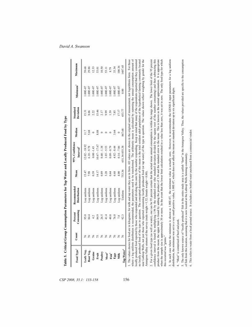
Discussion Study Recommendations Both sets of parameters, the reasonable conservative set and the bounding set, are found in Table 5. For the reasonable, conservative set, the parameters are given by the minimum and maximum values for use with a log-uniform distribution, while for the high bounding set, the parameters are given by the maximum values. For the high bounding set, the parameters Aare recommended to be considered as fixed, without a distribution. These parameters were duly supplied to the health physicists responsible for developing ingestion exposure estimates. Recommendations for Applied Demographers For applied demographers tasked with developing information, this case study suggests that a wide range of skills is needed in dealing with the identification of a population of interest. This is not a unique finding (Kintner et al., 1995; Murdock and Swanson, 2008; Pol and Thomas, 2001; Smith and McCarty, 1996). In this case, however, the population of interest is, indeed, a “special” one – extremely small in size, but with a huge impact. The identification of this population required not only knowledge of basic demographic methods and data sources, but a reasonable level of knowledge of both survey research methods and inferential statistics. Understanding what data were available from public sources what data needed to be collected also were important components in developing the information needed to complete the task.

The problem reported here is very different than the typical one facing most applied demographers. It asked for the identification of a “population” rather than an estimate (or forecast) of the size and composition of the population in a given geographic area. This can be taken as an example of the new types of challenges facing applied demography in the 21st century, some of which are listed by Swanson, Smith, and Tayman (2001). Further, as has been demonstrated by Smith and McCarty (1996) and Swanson et al. (2007) in regard

Tabl

e 5.

Cri

tical

Gro

up C

onsu

mpt

ion

Para

met

ers f

or T

ap W

ater

and

Loc

ally

Pro

duce

d Fo

od b

y Ty

pe

Lea

fy V

eg.

7695

.0Lo

g un

iform

15.4

712

.02

- 18.

9211

.715

.31

1.00

E-07

59.6

8R

oot V

eg.

7684

.4Lo

g un

iform

7.98

6.18

- 9.

78

5.68

8.06

1.00

E-07

29.8

6G

rain

s76

4.2

Log

unifo

rm0.

390.

00 -1

.43

02.

221.

00E-

0712

.33

Frui

t75

84.9

Log

unifo

rm14

.17

10.6

7 - 1

7.67

8.88

15.4

61.

00E-

0753

.01

Poul

try

7626

.5Lo

g un

iform

0.89

0.40

- 1.

380

2.17

1.00

E-07

10.5

0

Mea

t476

41.4

Log

unifo

rm3.

281.

03 -

5.53

09.

991.

00E-

0753

.11

Fish

576

40.8

Log

unifo

rm0.

440.

09 -

0.79

01.

591.

00E-

078.

79E

ggs

7676

.0Lo

g un

iform

6.68

4.92

- 8.

443.

647.

851.

00E-

0733

.34

Milk

767.

8Lo

g un

iform

4.00

0.14

- 7.

860

17.1

71.

00E-

0710

0.36

Tap

Wat

er6

7692

.3U

nifo

rm75

3.36

651.

34-8

55.3

886

7.68

453.

770.

0014

87.4

5

5.Th

eon

lykn

own

sour

ceof

“loc

ally

prod

uced

”fis

hin

the

entir

est

udy

area

isa

catfi

sh“f

arm

”in

theA

mar

gosa

Valle

y.Th

us,t

heva

lues

prov

ided

are

spec

ific

toth

eco

nsum

ptio

nof

fish

from

this

loca

tion,

ass

umin

g th

at it

is n

ow lo

cate

d at

the

Lath

rop

Wel

ls fa

rmin

g co

mm

unity

.6.

Thi

s ref

ers t

o w

ater

from

a lo

cal g

roun

d so

urce

. It

excl

udes

any

bot

tled

wat

er p

urch

ased

from

a c

omm

erci

al v

endo

r.

Med

ian

Stan

dard

D

evia

tion

Min

imum

3M

axim

um

1.Th

eva

lues

show

nfo

rfoo

dar

ein

kilo

gram

s;fo

rmilk

and

tap

wat

erth

eyar

ein

liter

s.A

llva

lues

are

show

nin

the

orig

inal

units

ofm

easu

rem

ent,

notl

ogar

ithm

icfo

rm.

Fort

hose

whe

rea

log

unifo

rmdi

strib

utio

nis

reco

mm

ende

d,th

epa

ram

eter

sne

edto

betra

nsfo

rmed

.Th

ear

ithm

etic

mea

nis

calc

ulat

edby

sum

min

gth

ean

nual

cons

umpt

ion

amou

ntof

loca

llypr

oduc

edfo

odre

porte

dby

thos

ew

hore

spon

ded

and

divi

ding

this

sum

byth

enu

mbe

rres

pond

ing.

Kee

pin

min

dth

atm

any

ofth

ere

spon

dent

sre

porte

dth

atth

eyco

nsum

edno

loca

llypr

oduc

edfo

odof

the

type

inqu

estio

n.Th

eco

ncep

tual

deno

min

ator

ofth

ism

ean

isth

eto

talr

esid

enta

dult

popu

latio

nof

the

hypo

thet

ical

farm

ing

com

mun

itylo

cate

dne

arLa

thro

pW

ells

,not

just

thos

ew

hore

porte

dco

nsum

ing

loca

llypr

oduc

edfo

od(o

rta

pw

ater

)of

the

type

inqu

estio

n.Th

eva

lues

show

nre

flect

wei

ghtin

gby

gend

erfo

rthe

Am

argo

sa V

alle

y st

ratu

m o

f the

surv

ey (m

ale

wei

ght =

1.32

; fem

ale

wei

ght =

0.8

0).

2.Fo

ragi

ven

food

type

(as

wel

las

wat

er),

one

can

be95

perc

entc

erta

inth

atth

eac

tual

mea

nan

nual

cons

umpt

ion

isw

ithin

the

rang

esh

own.

The

low

erlim

itof

the

95pe

rcen

tco

nfid

ence

inte

rval

isfo

und

bym

ultip

lyin

g1.

96by

the

stan

dard

erro

r(th

est

anda

rdde

viat

ion

divi

ded

byth

esq

uare

root

ofth

enu

mbe

rco

nsum

ing)

and

then

subt

ract

ing

this

prod

uctf

rom

the

mea

n;th

eup

perl

imit

isfo

und

byad

ding

the

prod

ucto

f1.9

6an

dth

est

anda

rder

rort

oth

em

ean.

This

iskn

own

asth

eno

rmal

appr

oxim

atio

n.It

isap

prop

riate

whe

nth

esa

mpl

esi

zeis

appr

oxim

atel

y30

orm

ore.

Inth

eev

entt

hatt

helo

wer

limit

calc

ulat

ion

resu

lted

ina

valu

ele

ssth

anze

ro,i

twas

sett

oze

ro.

The

only

food

type

forw

hich

this

occ

urre

d w

as "

grai

ns."

3.In

each

case

whe

reth

em

inim

umis

show

nas

1.00

E-07

,th

em

inim

umva

lue

isac

tual

lyze

ro.

How

ever

,to

acco

mm

odat

eth

eG

ENII

-Sin

putp

aram

eter

sfo

ra

log

unifo

rmdi

strib

utio

n, th

e m

inim

um w

as se

t to

a ve

ry sm

all p

ositi

ve v

alue

, 1.0

0E-0

7, w

hich

doe

s not

affe

ct th

e m

ean

or st

anda

rd d

evia

tion

up to

six

sign

ifica

nt d

igits

.4.

“M

eat”

is c

ompr

ised

of b

eef a

nd p

ork.

95%

Con

fiden

ce

Inte

rval

2 F

ood

Type

1C

ount

Perc

ent

Con

sum

ing

Rec

omm

ende

d D

istr

ibut

ion

Mea

n

David A. Swanson

156CSP 2008, 35.1: 133-158


CSP 2008, 35.1: 133-158

157

to estimating the demographic effects of natural disasters, the sequelae of September 11th, 2001 may foreshadow even more demanding challenges.

This case study not only underscores the importance of having team specialists in any major project who have common grounds of understanding, but gives an idea of the extreme data needs likely to be demanded of demographers in the 21st century. The demographer in this project had to communicate with health physicists, mathematicians, engineers, federal agency representatives, and appointed officials while working under tight time deadlines and the ubiquitous budget constraints. As such, budding applied demographers, especially those nearing completion of their graduate studies, should consider adopting a set of skills beyond traditional demography as opportunities present themselves (Morrison et al. 2000).

Acknowledgements: *An earlier version of this paper was presented at the 2002 annual meeting of the Population Association of America. The comments and suggestions received from participants are appreciated, particularly those from Tom Bryan. The author also appreciates the comments of two anonymous reviewers and Dr. Frank Trovato. Views presented are those of the author.

References: Dyer, J.R. 1999. "Interim Guidance Pending Issuance of New U.S. Nuclear

Regulatory Commission (NRC) Regulations for Yucca Mountain." Letter from J.R. Dyer (DOE/YMSCO) to D.R. Wilkins (CRWMS M&O), OL&RC:AVG:1435, June 18, 1999, with enclosure.

Hintze, J. 1995. NCSS 6.0 User's Guide. Kaysville, Utah: NCSS, Inc.

Kintner, H., T. Merrick, P. Morrison, and P. Voss. 1994. “Introduction” pp. 3-9 in H. Kintner, T. Merrick, P. Morrison, and P. Voss (Eds). Demographics: A Casebook for Business and Government. Boulder, CO: Westview Press.

Morrison, P. A., C. Popoff, I. Sharkova, D. Swanson, and J. Tayman. 2000. “Leveraging Extant Data to Meet Local Information Needs: A Case Study in Team Applied Demography.” Paper presented at the Annual Meeting of the Population Association of America. Los Angeles, California, March 23-25.

David A Swanson

CSP 2008, 35.1: 133-158

158

Pol, L. and R. Thomas. 2001. The Demography of Health and Health Care. 2nd

Edition. New York, NY: Kluwer Academic Publishers/Plenum Press. Smith, S. and C. McCarty. 1996. “Demographic Effects of Natural Disasters: A

Case Study of Hurricane Andrew. Demography 33 (2): 265-275.

SNL . 1993. User's Guide for GENII-S: A Code for Statistical and Deterministic Simulations of Radiation Doses to Humans from radionuclides in the Environment. SAND91-0561 UC-721. Albuquerque, NM: Sandia National Laboratories.

Swanson, D., S. Smith, and J. Tayman. 2001. “Population Projections for Small Areas: New Directions in the 21st Century.” Paper presented at the 4th International Nostradamus Conference on Prediction and Non-Linear Dynamics, Tomas Bata University, Zlin, Czech Republic, September 25-26.

Swanson, D., M. Van Boening, and R. Forgette. 2007. “Assessing Katrina’s Demographic and Social Impacts on the Mississippi Gulf Coast: Preliminary Results.” Paper presented at the annual meeting of the American Statistical Association, Salt Lake City, Utah, July 31st.

TRW. 1998. Yucca Mountain Site Characterization Project: Summary of

Socioeconomic Data Analyses Conducted In Support of The Radiological Monitoring Program, April 1997 to April 1998. June. Las Vegas, Nevada: TRW Environmental Safety Systems Inc.

U.S. DOE. 1997. The 1997 'Biosphere' Food Consumption Survey: Summary

Findings and Technical Documentation. Las Vegas, Nevada: U.S. Department of Energy, Office of Civilian Radioactive Waste Management.

U.S. DOE. 1998. Viability Assessment of a Repository at Yucca Mountain. Las

Vegas, Nevada. DOE/RW-0508. Las Vegas, Nevada: U.S. Department of Energy, Office of Civilian Radioactive Waste Management.

64 FR 8640. Disposal of High-Level Radioactive Waste in a Proposed

Geologic Repository at Yucca Mountain, Nevada. Proposed Rule 10 CFR 63. Washington, D.C.: National Archives and Records Administration.

Documents

Applied Demography In Action: A Case Study of … · posed to applied demographers by clients and users in the 21st century. As such, budding applied demographers, especially those