Embed Size (px)
Citation preview
Applied Mathematical Ecology/Ecological Modelling
Dr Hugh Possingham
The University of Queensland
(Professor of Mathematics and Professor of Ecology)
AMSI Winter School 2004

• Ecology and mathematics• Mathematics to design reserve systems• Mathematics to manage fire• Mathematics to manage populations• Mathematics to manage and learn
simultaneously• Optimisation, Markov chains
Overview

• Do “enough” to solve the problem
• What is interesting is not always important, what is important is not always interesting
• Unusual dynamic behaviour may well be just that - unusual
• The solution to our problems in science is not always to make more and more complex models.
• Reductionism vs Holism.
Take home messages
Optimal Reserve System Design
Hugh Possingham and Ian Ball (Australian Antarctic Division) and
others
History of reserve design
• Recreation
• What is left over
• Special features
• SLOSS and Island biogeography
• CAR reserve systems (Gap analysis)
• The minimum set problem

13,000 planning units

The “minimum set” problemHow do we get an efficient
comprehensive reserve system
• Minimise the “cost” of the reserve system
• Subject to the “constraints” that all biodiversity targets are met
• New age problems - add in spatial considerations, like total boundary length

Example Problem 1Find the smallest number of sites that represents all species
The data matrix - A
SITESPECIES A B C D E F G H RangePowerful Owl 1 1 1 1 1 1 0 1 7Red Goshawk 1 1 1 1 0 0 0 1 5Olive Whistler 1 1 0 1 1 1 0 0 5Albert's Lyrebird 1 1 1 0 0 0 1 1 5Coxen's Fig Parrot 1 1 1 1 0 0 1 0 5Diamond Firetail 1 0 0 0 1 1 1 0 4Black-b Button-quail 1 0 1 1 0 0 0 0 3Eastern Bristlebird 1 1 1 0 0 0 0 0 3Rufous Scrub-bird 0 1 0 0 1 0 0 0 2Ground Parrot 0 0 1 0 0 0 0 0 1Site Richness 8 7 7 5 4 3 3 3 40

Algorithms to solve the reserve system design problem
• Wild guess
• Heuristics
• Mathematical Programming
• Heuristic algorithms– Simulated annealing– Genetic Algorithms

Heuristics
• Richness algorithms
• Rarity algorithms
• Neither work so well with bigger data sets, especially where space is an issue
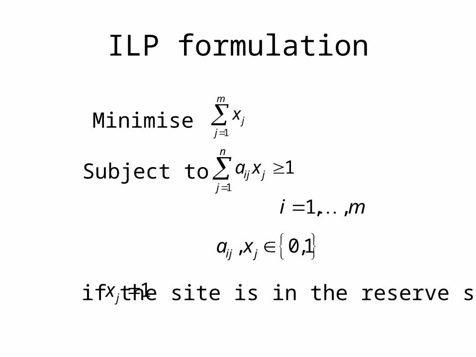
ILP formulation
1
m
jj
x
1
1n
ij jj
a x
1, ,i m
, 0,1ij ja x
Minimise
Subject to
1jx if the site is in the reserve system

Problem 2: Select the smallest set of the 12 sites below that conserves all species
SITE RaritySPECIES A B C D E F G H I J K L Rng ScorePowerful Owl 1 0 1 1 0 1 1 1 0 1 1 1 9 0.11Red Goshawk 1 0 0 1 1 1 1 1 1 0 1 1 9 0.11Pale Yellow Robin 1 1 1 1 1 0 0 1 1 0 0 1 8 0.13Albert's Lyrebird 1 1 0 1 1 1 1 0 1 0 0 0 7 0.14Coxen's Fig Parrot 1 0 1 1 0 0 0 0 0 0 1 1 5 0.20Diamond Firetail 0 0 1 1 0 0 1 1 0 0 1 0 5 0.20Black-b Button-quail 0 1 0 1 1 1 0 0 0 1 0 0 5 0.20Eastern Bristlebird 1 1 0 0 1 0 1 0 1 0 0 0 5 0.20Rufous Scrub-bird 1 0 0 0 0 0 1 0 0 1 1 0 4 0.25Black-throated Finch 1 0 1 1 0 0 0 1 0 0 0 0 4 0.25Star Finch 1 1 1 0 0 1 0 0 0 0 0 0 4 0.25Sthn Emu wren 1 0 1 0 0 1 0 0 0 0 0 0 3 0.33Glossy Back Cockatoo 0 1 0 0 1 0 0 0 1 0 0 0 3 0.33Diamond Firetail 0 1 0 0 0 1 0 0 0 1 0 0 3 0.33Black-chinned Honeyeater 0 1 0 0 0 0 0 0 0 1 0 0 2 0.50Riflebird 0 0 1 0 1 0 0 0 0 0 0 0 2 0.50Olive Whistler 0 0 0 0 0 0 0 1 1 0 0 0 2 0.50Ground Parrot 0 1 0 0 0 0 0 0 0 1 0 0 2 0.50Site Richness 10 9 8 8 7 7 6 6 6 6 5 4 82Rarity Score 2 2.6 2 1.3 1.6 1.5 1 1.3 1.4 1.9 0.9 0.5

Simulated annealingand Genetic Algorithms
We could “evolve” a good solution to the problem treating a reserve system like a piece of DNA. Fitness is a combination of number of sites plus a penalty for missing species. Fitness = - number of sites - 2xmissing species
If sites cost 1 and there is a 2 point penalty for missing a species then in problem 1 the “fitness” of the system {A,B,D} = - 3 - 2 = - 5 Which is not as fit as {A,B} = - 2 - 2 = - 4 or {A,B,C} = - 3 = - 3With best solution {C,E} = - 2 - 0 = - 2

GAs: Breeding a reserve system
2 4 7 8 20 25 28 cost 7 3 7 8 10 11 12 cost 6...
babies2 4 7 10 11 12 infeasible3 7 8 20 25 28 cost 6 ...

Simulated annealing
A genetic algorithm with no recombination,only point mutations and a population size of 1.
Selection process allows a decrease in fitness at the start of the process
Relies on speed and placing constraints in theobjective function

Objectives and constraints
• Typical constraints are to meet a variety of conservation targets – eg 30% of each habitat type or enough area for 2000 elephants (not just get one occurrence)
• Typical objectives are to satisfy the constraints while minimising the total “cost” (which may be area, actual cost, management cost, cost of rehabilitation)
• Objectives and constraints are somewhat interchangeable

Spatial problems
• There is more to the cost of a reserve system than its area
• Boundary length and shape are important
• Other rules about minimising boundary length, cost of land, forgone development opportunties, minimum reserve size, issues of adequacy
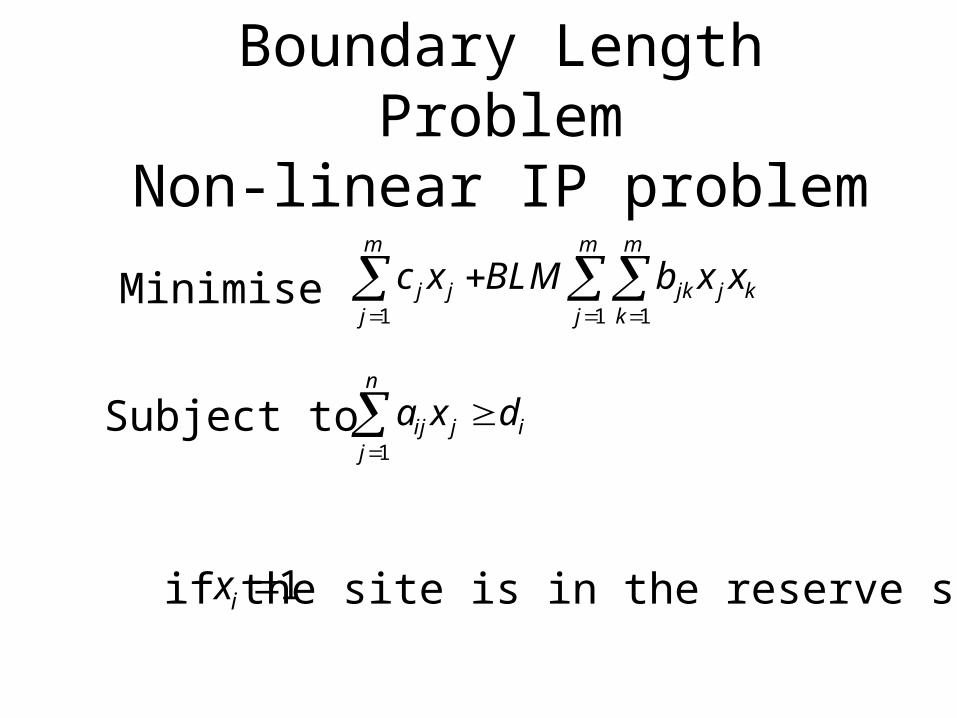
1 1 1
m m m
j j jk j kj j k
c x BLM b x x
Minimise
1ix if the site is in the reserve system
Boundary Length ProblemNon-linear IP problem
1
n
ij j ij
a x d
Subject to


Example 1: The GBR
• Divided in to hexagons
• 70 different bioregions (reef and non-reef)
• 13,000 planning units
• What is an appropriate target?
• What are the costs?
• Replication and
minimum reserve size• www.ecology.uq.edu.au/marxan.htm


The GBR process
• Determine optimal system based on ecological principles alone
• For low % targets there are many many options
• Introduce socio-economic data• Special places, targets, industry goals,
community aspirations• Delivered decision support by providing
options

The consequences of not planning
• The South Australian dilemma – of 18 reserves (4% by area), 9 add little to the goal of comprehensiveness (Stewart et al in press), they are effectively useless in the context of a well defined problem even if targets are 50% of every feature type!
• Complimentarity is the key• The whole is more than the sum of the parts

Legend
Existing Marine Reserves
No Reserves @ 10% Target
Reserves Fixed @ 10% Target
Effect of South Australia’s existing marine reserves

But reserve systems arenot built in a day
• Idea of irreplaceability introduced to deal with the notion that when some sites are lost they are more (or less) irreplaceable (Pressey 1994).
• The irreplaceability of a site is a measure of the fraction of all reserve systems options lost if that particular site is lost
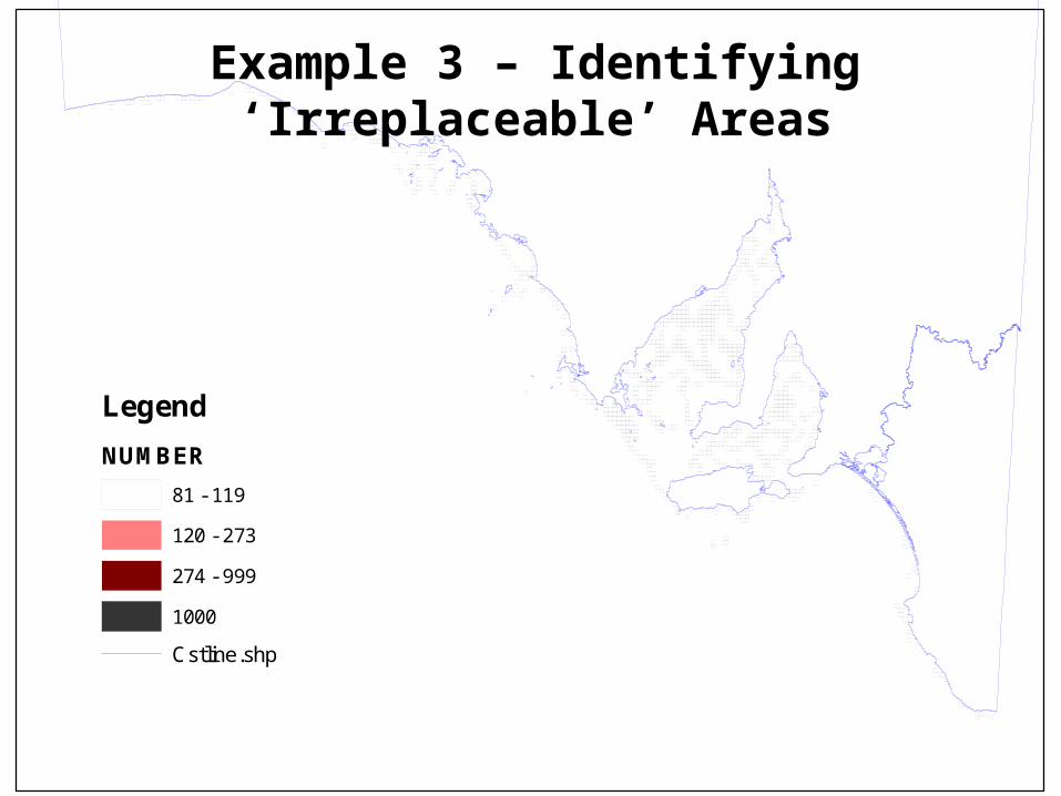
Legend
NUMBER
81 - 119
120 - 273
274 - 999
1000
Cstline.shp
Example 3 – Identifying ‘Irreplaceable’ Areas
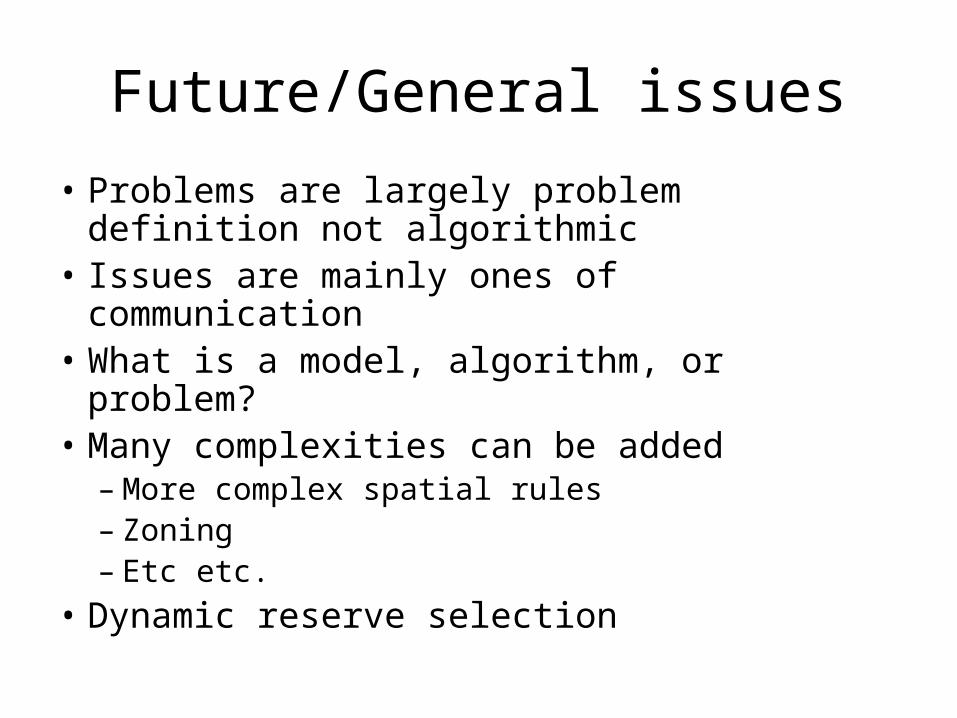
Future/General issues
• Problems are largely problem definition not algorithmic
• Issues are mainly ones of communication• What is a model, algorithm, or problem?• Many complexities can be added
– More complex spatial rules– Zoning– Etc etc.
• Dynamic reserve selection
Optimal Fire Management
for biodiversity conservation
Hugh Possingham, Shane Richards, James Tizard and Jemery Day
The University of Queensland/Adelaide
NCEAS - Santa Barbara

What is decision theory?
• Set a clear objective
• Define decision variables - what do you control?
• Define system dynamics including state variables and constraints

The problem
• How should I manage fire in Ngarkat Conservation Park - South Australia?
• What scale?
• What biodiversity?
• How is it managed now?
• What is the objective?

Vegetation
• Dry sandplain heath (like chapparal) - 300mm, winter rainfall
• Little heterogeneity in soil type or topography - poor soils
• Diverse shrub layer with some mallee
• Key species - Banksia, Callitris, Melaleuca, Leptospermum, Hibbertia, Eucalyptus

Habitat

Assume three successional states
early
late
mid
fire, f
1/se
1/sm

Ngarkat Conservation Park

Nationally threatened bird species
• Slender-billed Thornbill - early
• Rufous Fieldwren - early
• Red-lored Whistler - mid
• Mallee Emu-wren - mid/late
• Malleefowl - late
• Western Whipbird - late

0
0.1
0.2
0.3
0.4
0.5
0.6
0 5 10 15 20 25 30 35 40 45 50 55
% of Ngarkat CP burnt each year by wildfire
Pro
ba
bilit
yNgarkat data, 1976-1992
All wildfires are left toburn unhinderedAll wildfires are fought

# MidSites
201918171615 ZERO OLD SITES
1413121110
98
7 GOOD
6 STATES
54
32
1
0 0 2 4 6 8 10 12 14 16 18 20
# Early Sites
State space and dynamics

Vegetation dynamics:Transition probability from j early to i early
E i j
s s i jj ij j i i
e e if
otherwise.
1
0

Fire model
otherwise,0
and if)(
,ijij
e
lmnNn
ll
mm
elmn
nji
llmmfF
i jjj
Probability system moves from state(ej,mj,lj) to state (ei,mi,li) due to fire
Where fn is the probability of afire that hits n patches
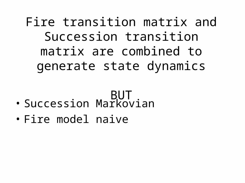
Fire transition matrix and Succession transition matrix are combined to
generate state dynamics
BUT• Succession Markovian
• Fire model naive

The optimization problem
• Objective - 20% each stage• State space - % of park in each
successional stage• Control variable - given the current
state of park should you do nothing,fight fires, start fires?
• System dynamics determined by transition matrices

Solution method
• Stochastic dynamic programming (SDP)
• Optimal solution without simulation but can be hard to determine
• Only works with a relatively small state space - (Nx(N+1))/2

# MidSites
201918171615 ZERO OLD SITES
1413121110
98
7 GOOD
6 STATES
54
32
1
0 0 2 4 6 8 10 12 14 16 18 20
# Early Sites
State space and dynamics

# MidSites
20191817 FIGHT WILDFIRES
16 DO NOTHING
15 BURN
1413121110
9876543210
0 2 4 6 8 10 12 14 16 18 20
# Early Sites
Optimal strategy with no costs

# MidSites
20191817 FIGHT WILDFIRES
16 DO NOTHING
15 BURN
1413121110
9876543210
0 2 4 6 8 10 12 14 16 18 20
# Early Sites
Optimal strategy with costs
Conclusion
• Decision is state-dependent - there is no simple rule
• Costs may be important
• The decision theory framework allows us to address the problem and find a solution
• Details - Richards, Possingham and Tizard (1999) - Ecological Applications

Where are we going?
• Rules of thumb - depend on the intervals between successional states and fire frequency (Day)
• Spatial version (Day)
• More detailed vegetation and animal population models

Eradicate, Exploit, Conserve
Decision TheoryPure Ecological Theory
Applied
Theoretical
Ecology
+
=
How to manage a metapopulation
Michael Westphal (UC Berkeley),
Drew Tyre (U Nebraska), Scott Field (UQ)
Can we make metapopulation theory useful?

Specifically: how to reconstruct habitat for a small metapopulation
• Part of general problem of optimal landscape design – the dynamics of how to reconstruct landscapes
• Minimising the extinction probability of one part of the Mount Lofty Ranges Emu-wren population.
• Metapopulation dynamics based on Stochastoc Patch Occupancy Model (SPOM) of Day and Possingham (1995)
• Optimisation using Stochastic Dynamic Programming (SDP) see Possingham (1996)
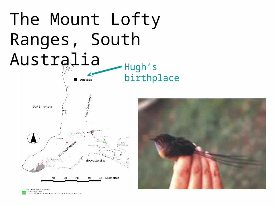
The Mount Lofty Ranges, South Australia
Hugh’s birthplace

MLR Southern Emu Wren
• Small passerine (Australian malurid)
• Very weak flyer
• Restricted to swamps/fens
• Listed as Critically Endangered subspecies
• About 450 left; hard to see or hear
• Has a recovery team (flagship)

The Cleland Gully
Metapopulation;
basically isolated
Figure shows options
Where should we revegetate now, and in the future? Does it depend on the state of the metapopulation?

Stochastic Patch Occupancy Model(Day and Possingham, 1995)
State at time, t, (0,1,0,0,1,0)
Intermediate states
State at time, t+1, (0,1,1,0,1,0)
(0,0,0,0,1,0)
Extinction process
Colonization process
(0,1,0,0,1,0)
(0,1,0,0,0,0)
Plus fire

The SPOM
• A lot of “population” states, 2n, where n is the number of patches. The transition matrix is 2n by 2n in size (128 by 128 in this case).
• A “chain binomial” model (Possingham 96, 97; Hill and Caswell 2001?)
• SPOM has recolonisation and local extinction where functional forms and parameterization follow Moilanen and Hanski
• Overall transition matrix, a combination of extinction and recolonization, depends on the “landscape state”, a consequence of past restoration activities
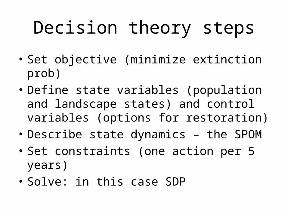
Decision theory steps
• Set objective (minimize extinction prob)
• Define state variables (population and landscape states) and control variables (options for restoration)
• Describe state dynamics – the SPOM
• Set constraints (one action per 5 years)
• Solve: in this case SDP

Control options (one per 5 years, about 1ha reveg)
E5: largest patch bigger, can do 6 times
E2: most connected patch bigger, 6 times
C5: connect largest patch
C2: connect patches1,2,3
E7: make new patch
DN: do nothing

E5E5E5E5E5
Management trajectories:1 – only largest patch occupied
C5
E5
E7
DN

E5E5E5E5
Management trajectories:2 – all patches occupied
C2E2
E7DNE5
E5E5E2 C5
E2
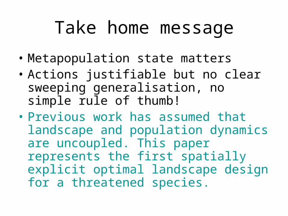
Take home message
• Metapopulation state matters• Actions justifiable but no clear sweeping
generalisation, no simple rule of thumb!• Previous work has assumed that
landscape and population dynamics are uncoupled. This paper represents the first spatially explicit optimal landscape design for a threatened species.
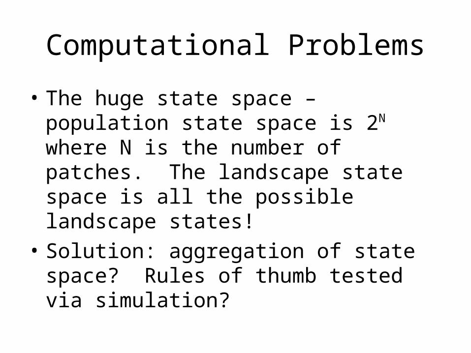
Computational Problems
• The huge state space – population state space is 2N where N is the number of patches. The landscape state space is all the possible landscape states!
• Solution: aggregation of state space? Rules of thumb tested via simulation?

Other applications of decision theory to population management
and conservation• Optimal metapopulation management (Possingham 96, 97;
Haight et al 2002)• Optimal fire management (Possingham and Tuck 98, Richards et
al 99, McCarthy et al. 01)• Optimal biocontrol release (Shea and Possingham, 00)• Optimal landscape reconstruction (Westphal et al., submitted)• Optimal captive breeding management (Tenhumberg et al, to
submit)• Optimal weed management (Moore and Possingham, to submit)• Decision theory and PVA/conservation (Possingham et al. – 01,
02 book chapters) – The Business of Biodiversity• Optimal Reserve System Design, MARXAN, TNC (several
papers)

Optimal translocation strategies
Consider the Arabian Oryx Oryx leucoryx – if we know how many are in the wild, and in a zoo, and we know birth and death rates in the zoo and the wild, how many should we translocate to or from the wild to maximise persistence of the wild population
Brigitte Tenhumberg, Drew Tyre (U Nebraska), Katriona Shea (Penn State)

Oryx problem
Zoo Population
Growth rate R = 1.3 Capacity = 20
Wild Population
??
Growth rate R = 0.85 Capacity = 50

Result – base parameters
Captive Population
Wild
Pop
ulat
ion
C
R
Captive Population
Wild
Pop
ulat
ion
C
R
R = release, mainly when population in zoo is near capacityC = capture, mainly when zoo population small, capture entire wild population when this would roughly fill the zoo

If zoo growth rate changes, results change – but for a “new” species we
won’t know R in the zoo
Enter – active adaptive management,Management with a plan for learning

Active adaptive management
• Management of uncertain stochastic systems with a plan for learning
• How do you trade-off the need to optimally manage a system with the information gain you need to manage that same system
Cindy Hauser, Petra Kuhnert, Katriona Shea, Tony Pople, Niclas Jonzen (Lund)

Toy fish problem
Secure
Collapsed
Fragile
Secure
Fragile
Collapsed
Unharvested Harvested
????? ?????
Harvest,Harvest,
Yes or no?Yes or no?
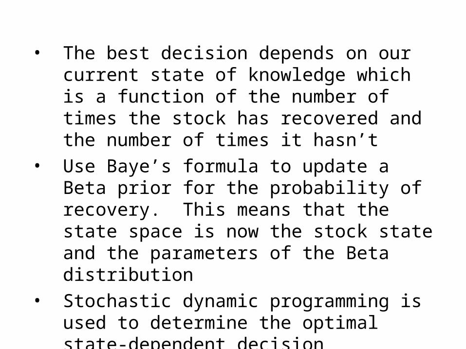
• The best decision depends on our current state of knowledge which is a function of the number of times the stock has recovered and the number of times it hasn’t
• Use Baye’s formula to update a Beta prior for the probability of recovery. This means that the state space is now the stock state and the parameters of the Beta distribution
• Stochastic dynamic programming is used to determine the optimal state-dependent decision
• Cindy is now applying to kangaroos with a large population state space

Active adaptive monitoring: the problem of the Swedish lynx Lynx lynx
• The toy fish problem assumes that we know the size of the fish stock. Now assume that we do know the system dynamics, but we have to spend money monitoring to determine the population size which then determines the harvesting strategy
• How much money do we spend monitoring and is optimal monitoring state dependent??
Henrik Andren (SLU), Anna Daniel (SLU), Cindy Hauser, Tony Pople

Information for Swedish lynx problem
• “Population size” (N) is number of Lynx family units• Compensation cost per N – 20,000 SK, higher if N > 200• Cost of current monitoring program• Political cost of N falling below 50 = 100,000,000 SK• Fixed harvest strategy – 15% if N > 80, 0% otherwise• Growth rate R – normally distributed (mean 1.17)• Monitoring strategies:
– M1 – cost 2,000,000 SK and generates N with a SD of 0.1N– M2 – cost ? SK generates N with a SD of 0.3N– (M0 – no count, cost 0, estimate based on last year and mean
growth rate

Results – should monitoring bestate-dependent?
Utility 106
Number of Lynx family units (N)
10
100
40
50 200
States of intensive monitoring?

Applied Theoretical Ecologist Dreaming
Optimal Harvesting
Optimal Monitoring
Optimal Learning

New approaches to the “evolution” of complex ecological systems: kangaroo
population dynamics
PIs: Hugh Possingham, Gordon Grigg,
Stuart Phinn, Clive McAlpine
PDFs: Tony Pople, Niclas Jonzén,
Brigitte Tenhumberg
PhDs: Cindy Hauser, Norbert Menke
Money: ARC Linkage, UQ, Environment Australia, DEH (SA), EPA (QLD), MDBC, Packer Tanning
What is important is
not always interestin
g,
What is interestin
g is not always im
portant

Overview1. Background and History
2. Visualisation of the patterns
3. The confrontation of models with data
4. Why model – prediction, utility or understanding?
5. The evolutionary impact of harvesting – a “just so”
story
6. Optimal adaptive monitoring
7. Learning while managing – a new discipline - applied
theoretical ecology

1 Background and History• Data collected from 1978
• Kangaroo quotas, 15% of the estimates
• Previous mathematical modeling, single spatial scale with a short time series
• Few other population studies on a large scale – locusts, phytoplankton
• Harvesting theory typically for fish only

Data collection: Fixed-wing Survey

2 Visualisation of the patterns
• With complex ecological systems visualising the data can be an important part of understanding and theorising
• Aside from kangaroo numbers we have – rainfall data– National Digitised Vegetation Index (NDVI, satellite)
data– sheep data– pasture biomass models, and– harvest data
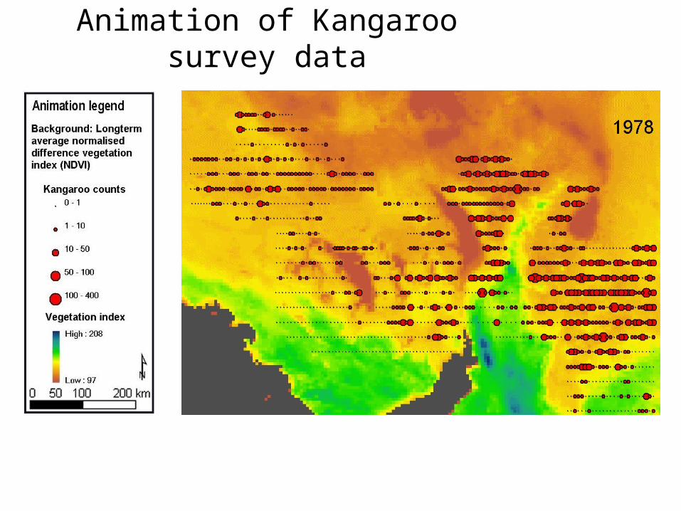
Animation of Kangaroo survey data

Temporal patterns at a whole region scale
0
5
10
15
20
25
1980 1985 1990 1995 2000 2005
Sca
led
mea
sure
Year
Kangaroo Numbers
Vegetation Index
Growth Rate
??

3 The confrontation of model with data
• Is rainfall a good surrogate for resources?
• What is the most plausible time lag?
• How does density dependence work if at all?
• Do sheep compete with kangaroos?
• Are there environmental correlations between
regions?

South Australia: main management zones
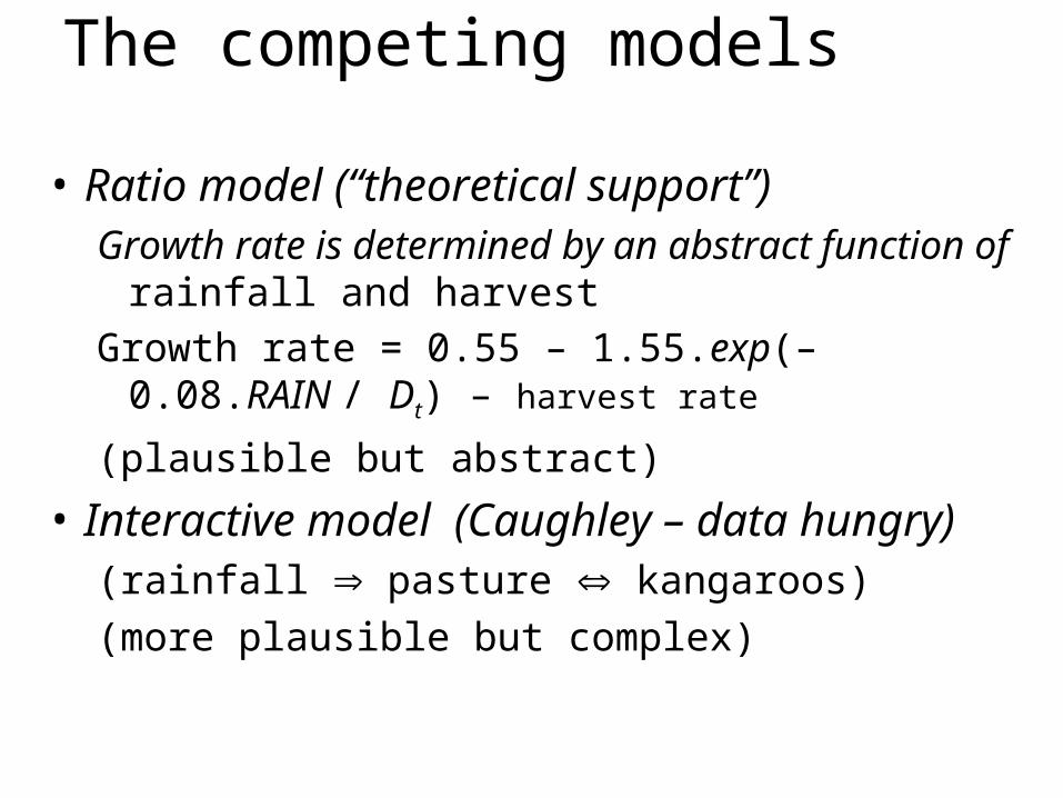
The competing models
• Ratio model (“theoretical support”)Growth rate is determined by an abstract function
of rainfall and harvest
Growth rate = 0.55 – 1.55.exp(– 0.08.RAIN / Dt) – harvest rate
(plausible but abstract)
• Interactive model (Caughley – data hungry)(rainfall pasture kangaroos)
(more plausible but complex)

Ratio Model
0
5
10
15
20
25
1976 1980 1984 1988 1992 1996 2000 2004
Modelled population
Actual population
Northeast Pastoral Zone
Year
Pop
ulat
ion
size

Interactive model
Northeast Pastoral Zone
0.0000
0.0500
0.1000
0.1500
0.2000
0.2500
1976 1980 1984 1988 1992 1996 2000 2004
Pastu
re b
iom
ass (
kg
/ha)
Modelled population
Actual population
Pop
ulat
ion
size
Year

A more complex statistical model
The model – with nested effects of
1. density dependence – bN
2. rainfall – R
3. sheep – S
4. harvesting – H, and
5. correlated environmental variability, E
)()1(,)(,
)(,)(,)1(,)1(,)1(, tititiitiitiii EHSdRcNbatiti eNN

We don’t know as much as we thought
• Use Akaike’s information criteria to select the
most parsimonious model
• Best model, 50% support, suggests
– There is strong density dependence
– Harvesting matters, BUT
– Kangaroos eat sheep
– There are correlations between the regions not
explained by rainfall

Why model – prediction understanding or utility?
• Prediction – forecasting the future accurately
• Understanding – increase in knowledge, easy
to explain, mechanisms
• Utility – making good management decisions,
who cares if we understand

Optimal Harvest Strategy?
Logistic model, fish
0.00
0.20
0.40
0.60
0.80
1.00
1.20
1.40
1.60
0 10 20 30 40 50 60
Harvest rate (%)
Mea
n s
easo
nal
har
vest
km
-2
Ratio model
Interactive model
Mea
n ne
t har
vest
per
yea
r
Percentage harvest

Learning, monitoring and managing
• Management ultimately needs robust
predictive models, but which model?
• Can you monitor and manage to increase the
rate at which you refine your model choice?
• For example to learn more maybe we should
vary the harvesting and monitoring = active
adaptive monitoring/management

Monitoring and managing
0.0
0.1
0.2
0.4
0.5
0 1 2 3 4 5
250
300
350
400
450
500
Period of monitoring (years)
InfrequentAnnual
Probability of c
ollapse
Pro
babi
lity
of
coll
apse
Cost of m
onitoring $1000
Cost

Conclusion
• A diversity of novel methodologies
– Visualisation
– Simulation models
– Statistical models
– Process models
– Analysis in space and time
• An emphasis on confronting alternative models with data
• Applied Theoretical Ecology – new field and approach?

• Do “enough” to solve the problem: you can put a nail in a wall with a frying pan but frying pans are better for cooking
• What is interesting is not always important, what is important is not always interesting
• There are several reasons why one might want to construct a model
• The solution to our problems in science is not always to make more and more complex models.
• Reductionism vs Holism• The complex systems band wagon• Philosophy and ethics – why do you do what you do?
Take home messages