Embed Size (px)
Citation preview
Applied Nonparametric Bayes
Michael I. Jordan
Department of Electrical Engineering and Computer Science
Department of Statistics
University of California, Berkeley
http://www.cs.berkeley.edu/∼jordan
Acknowledgments: Yee Whye Teh, Romain Thibaux, Erik
Sudderth
1
Computer Science and Statistics
• Separated in the 40’s and 50’s, but merging in the 90’s and 00’s
• What computer science has done well: data structures and algorithms formanipulating data structures
• What statistics has done well: managing uncertainty and justification ofalgorithms for making decisions under uncertainty
• What machine learning attempts to do: hasten the merger along
– machine learning isn’t a new field per se
2
Computer Science and Statistics
• Separated in the 40’s and 50’s, but merging in the 90’s and 00’s
• What computer science has done well: data structures and algorithms formanipulating data structures
• What statistics has done well: managing uncertainty and justification ofalgorithms for making decisions under uncertainty
• What machine learning attempts to do: hasten the merger along
– machine learning isn’t a new field per se
• An issue to be grappled with: the two flavors of statistical inference(frequentist and Bayesian)
3
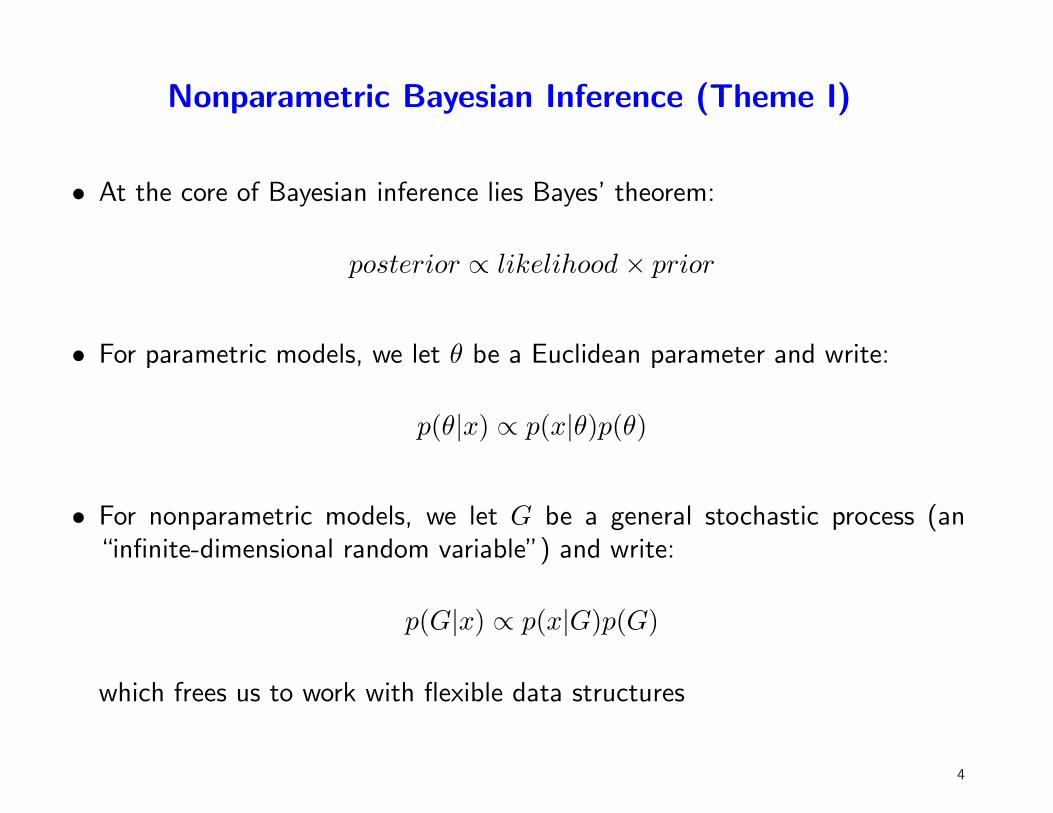
Nonparametric Bayesian Inference (Theme I)
• At the core of Bayesian inference lies Bayes’ theorem:
posterior ∝ likelihood × prior
• For parametric models, we let θ be a Euclidean parameter and write:
p(θ|x) ∝ p(x|θ)p(θ)
• For nonparametric models, we let G be a general stochastic process (an“infinite-dimensional random variable”) and write:
p(G|x) ∝ p(x|G)p(G)
which frees us to work with flexible data structures
4
Nonparametric Bayesian Inference (cont)
• Examples of stochastic processes we’ll mention today include distributionson:
– directed trees of unbounded depth and unbounded fan-out– partitions– sparse binary infinite-dimensional matrices– copulae– distributions
• General mathematical tool: completely random processes
5
Hierarchical Bayesian Modeling (Theme II)
• Hierarchical modeling is a key idea in Bayesian inference
• It’s essentially a form of recursion
– in the parametric setting, it just means that priors on parameters canthemselves be parameterized
– in our nonparametric setting, it means that a stochastic process can haveas a parameter another stochastic process
• We’ll use hierarchical modeling to build structured objects that arereminiscent of graphical models—but are nonparametric
– statistical justification—the freedom inherent in using nonparametricsneeds the extra control of the hierarchy
6
What are “Parameters”?
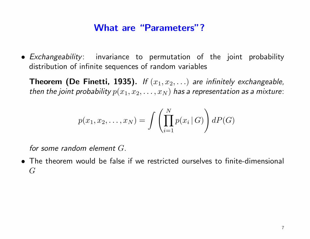
• Exchangeability : invariance to permutation of the joint probabilitydistribution of infinite sequences of random variables
Theorem (De Finetti, 1935). If (x1, x2, . . .) are infinitely exchangeable,
then the joint probability p(x1, x2, . . . , xN) has a representation as a mixture:
p(x1, x2, . . . , xN) =
∫
(
N∏
i=1
p(xi |G)
)
dP (G)
for some random element G.
• The theorem would be false if we restricted ourselves to finite-dimensionalG
7
Computational Consequences
• Having infinite numbers of parameters is a good thing; it avoids placingartificial limits on what one can learn
• But how do we compute with infinite numbers of parameters?
• Important relationships to combinatorics
8
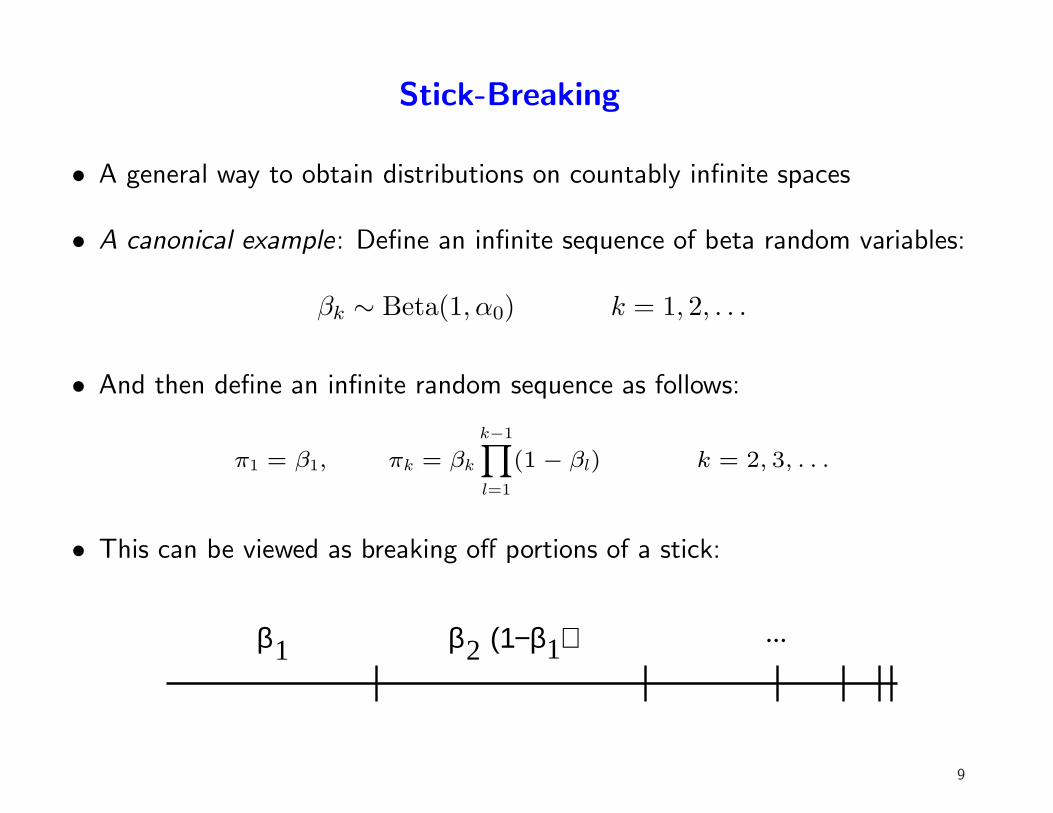
Stick-Breaking
• A general way to obtain distributions on countably infinite spaces
• A canonical example: Define an infinite sequence of beta random variables:
βk ∼ Beta(1, α0) k = 1, 2, . . .
• And then define an infinite random sequence as follows:
π1 = β1, πk = βk
k−1Y
l=1
(1 − βl) k = 2, 3, . . .
• This can be viewed as breaking off portions of a stick:
1 2...
1β β (1−β )
9
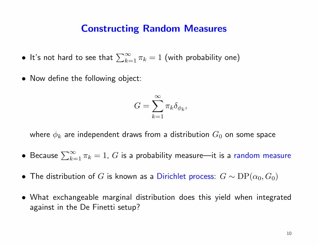
Constructing Random Measures
• It’s not hard to see that∑∞
k=1 πk = 1 (with probability one)
• Now define the following object:
G =∞∑
k=1
πkδφk,
where φk are independent draws from a distribution G0 on some space
• Because∑∞
k=1 πk = 1, G is a probability measure—it is a random measure
• The distribution of G is known as a Dirichlet process: G ∼ DP(α0, G0)
• What exchangeable marginal distribution does this yield when integratedagainst in the De Finetti setup?
10
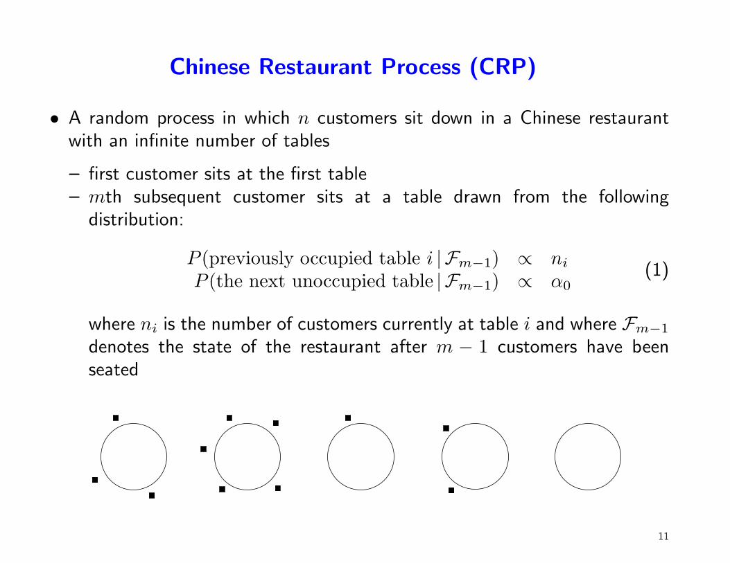
Chinese Restaurant Process (CRP)
• A random process in which n customers sit down in a Chinese restaurantwith an infinite number of tables
– first customer sits at the first table– mth subsequent customer sits at a table drawn from the following
distribution:
P (previously occupied table i | Fm−1) ∝ ni
P (the next unoccupied table | Fm−1) ∝ α0(1)
where ni is the number of customers currently at table i and where Fm−1
denotes the state of the restaurant after m − 1 customers have beenseated
��������
�� ����
��������
������������
����
��
��������
������
11
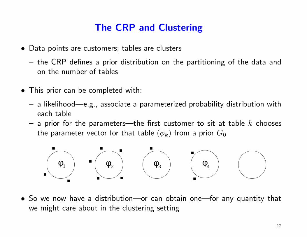
The CRP and Clustering
• Data points are customers; tables are clusters
– the CRP defines a prior distribution on the partitioning of the data andon the number of tables
• This prior can be completed with:
– a likelihood—e.g., associate a parameterized probability distribution witheach table
– a prior for the parameters—the first customer to sit at table k choosesthe parameter vector for that table (φk) from a prior G0
φ2φ1 φ3 φ��
�� ����
����
��������
��������
����
����
����
��
4
• So we now have a distribution—or can obtain one—for any quantity thatwe might care about in the clustering setting
12
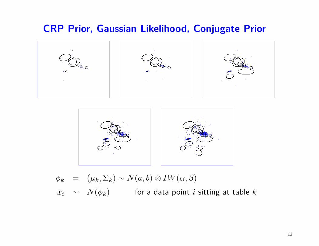
CRP Prior, Gaussian Likelihood, Conjugate Prior
φk = (µk, Σk) ∼ N(a, b) ⊗ IW (α, β)
xi ∼ N(φk) for a data point i sitting at table k
13
Posterior Inference for the CRP
• We’ve described how to generate data from the model; how do we gobackwards and generate a model from data?
• A wide variety of variational, combinatorial and MCMC algorithms havebeen developed
• E.g., a Gibbs sampler is readily developed by using the fact that the Chineserestaurant process is exchangeable
– to sample the table assignment for a given customer given the seating ofall other customers, simply treat that customer as the last customer toarrive
– in which case, the assignment is made proportional to the number ofcustomers already at each table (cf. preferential attachment)
– parameters are sampled at each table based on the customers at thattable (cf. K means)
• (This isn’t the state of the art, but it’s easy to explain on one slide)
14
Exchangeability
• As a prior on the partition of the data, the CRP is exchangeable
• The prior on the parameter vectors associated with the tables is alsoexchangeable
• The latter probability model is generally called the Polya urn model. Lettingθi denote the parameter vector associated with the ith data point, we have:
θi | θ1, . . . , θi−1 ∼ α0G0 +
i−1∑
j=1
δθj
• From these conditionals, a short calculation shows that the joint distributionfor (θ1, . . . , θn) is invariant to order (this is the exchangeability proof)
• As a prior on the number of tables, the CRP is nonparametric—the numberof occupied tables grows (roughly) as O(log n)—we’re in the world ofnonparametric Bayes
15
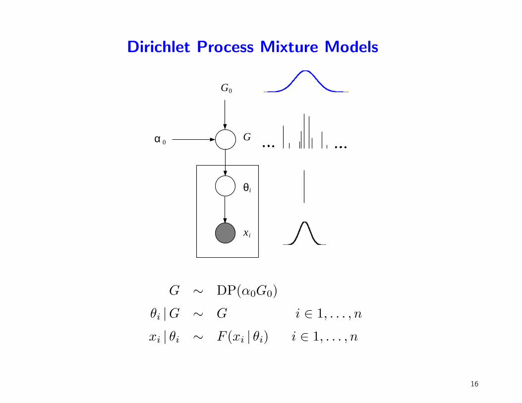
Dirichlet Process Mixture Models
Gα 0
G0
θi
xi
G ∼ DP(α0G0)
θi |G ∼ G i ∈ 1, . . . , n
xi | θi ∼ F (xi | θi) i ∈ 1, . . . , n
16
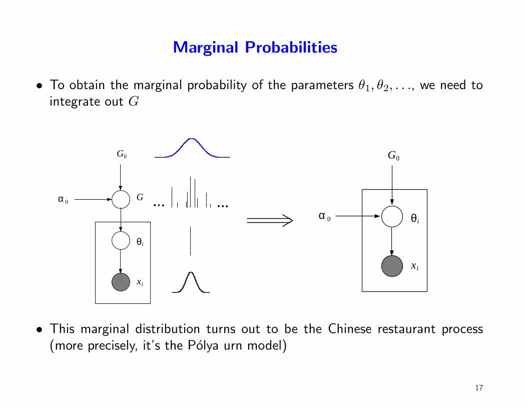
Marginal Probabilities
• To obtain the marginal probability of the parameters θ1, θ2, . . ., we need tointegrate out G
Gα 0
G0
θi
xi
α 0
G0
θi
xi
• This marginal distribution turns out to be the Chinese restaurant process(more precisely, it’s the Polya urn model)
17
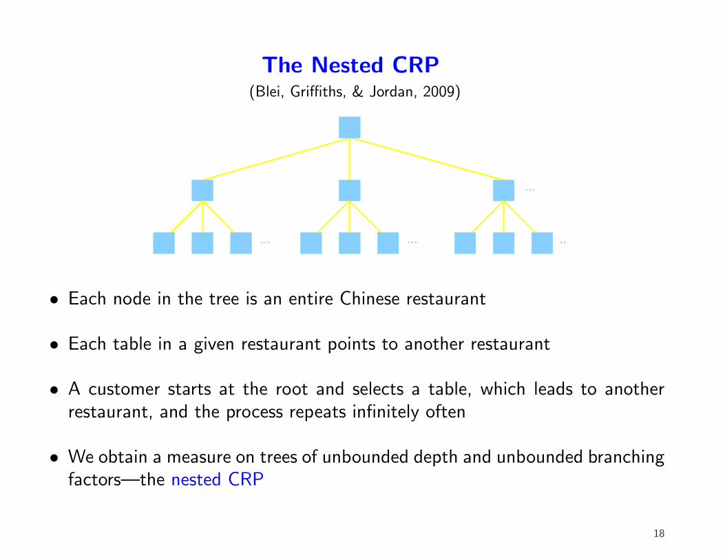
The Nested CRP(Blei, Griffiths, & Jordan, 2009)
... ...
...
...
• Each node in the tree is an entire Chinese restaurant
• Each table in a given restaurant points to another restaurant
• A customer starts at the root and selects a table, which leads to anotherrestaurant, and the process repeats infinitely often
• We obtain a measure on trees of unbounded depth and unbounded branchingfactors—the nested CRP
18
Hierarchical Topic Models(Blei, Griffiths, & Jordan, 2008)
• The nested CRP defines a distribution over paths in a tree
• At every node in the tree place a distribution on words (a “topic”) drawnfrom a prior over the vocabulary
• To generate a document:
– pick a path down the infinite tree using the nested CRP– repeatedly∗ pick a level using the stick-breaking distribution∗ select a word from the topic at the node at that level in the tree
19
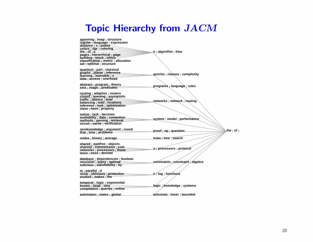
Topic Hierarchy from JACM
the ; of ; a
n ; algorithm ; time
spanning ; heap ; structureregular ; language ; expressiondistance ; s ; pointscolors ; dgr ; coloringthe ; of ; apages ; hierarchical ; pagebuilding ; block ; whichclassification ; metric ; allocationset ; optimal ; structure
queries ; classes ; complexityquantum ; part ; classicalgraphs ; planar ; inferencelearning ; learnable ; cdata ; access ; overhead
programs ; language ; rulesabstract ; program ; theorysets ; magic ; predicates
networks ; network ; routing
routing ; adaptive ; routersclosed ; queuing ; asymptotictraffic ; latency ; totalbalancing ; load ; locationsinference ; task ; optimizationclass ; have ; property
system ; model ; performanceonline ; task ; decisionavailability ; data ; contentionmethods ; parsing ; retrievalcircuit ; cache ; verification
proof ; np ; questionzeroknowledge ; argument ; roundthat ; time ; problems
trees ; tree ; searchnodes ; binary ; average
n ; processors ; protocolshared ; waitfree ; objectschannel ; transmission ; costnetworks ; processors ; thosemore ; trees ; derived
constraints ; constraint ; algebradatabase ; dependencies ; booleanrecursion ; query ; optimalsubclass ; satisfiability ; by
n ; log ; functionsm ; parallel ; dshow ; oblivious ; protectionstudied ; makes ; the
logic ; knowledge ; systemstemporal ; logic ; exponentialknown ; large ; verycompilation ; queries ; online
automata ; lower ; boundedautomaton ; states ; global
20
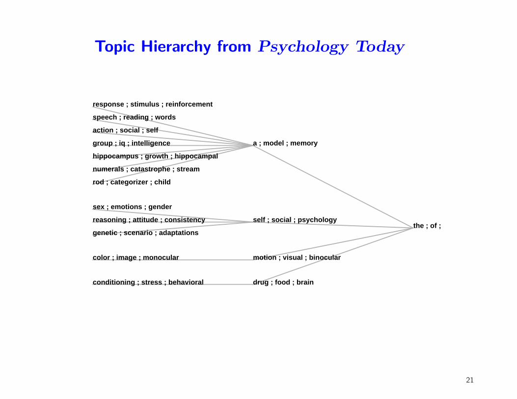
Topic Hierarchy from Psychology Today
the ; of ; and
a ; model ; memory
response ; stimulus ; reinforcement
speech ; reading ; words
action ; social ; self
group ; iq ; intelligence
hippocampus ; growth ; hippocampal
numerals ; catastrophe ; stream
rod ; categorizer ; child
self ; social ; psychology
sex ; emotions ; gender
reasoning ; attitude ; consistency
genetic ; scenario ; adaptations
motion ; visual ; binocularcolor ; image ; monocular
drug ; food ; brainconditioning ; stress ; behavioral
21
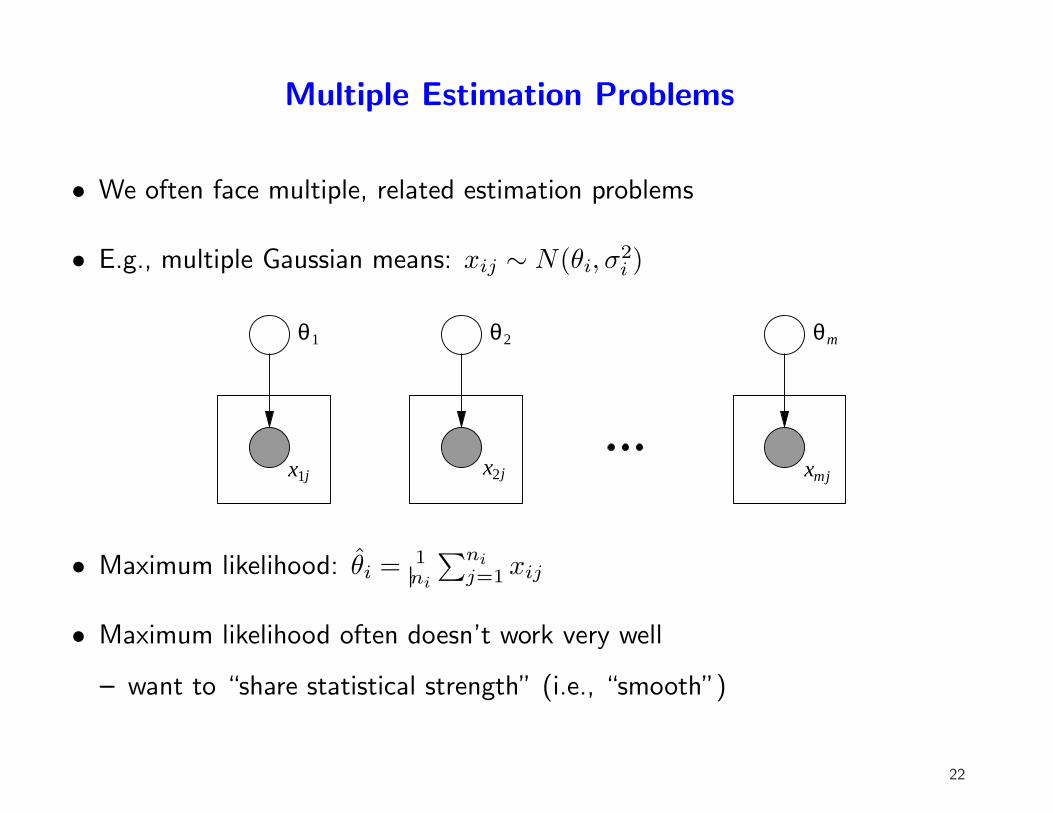
Multiple Estimation Problems
• We often face multiple, related estimation problems
• E.g., multiple Gaussian means: xij ∼ N(θi, σ2i )
2 θm1
x2 xmjjx1j
θ θ
• Maximum likelihood: θi = 1ni
∑nij=1 xij
• Maximum likelihood often doesn’t work very well
– want to “share statistical strength” (i.e., “smooth”)
22
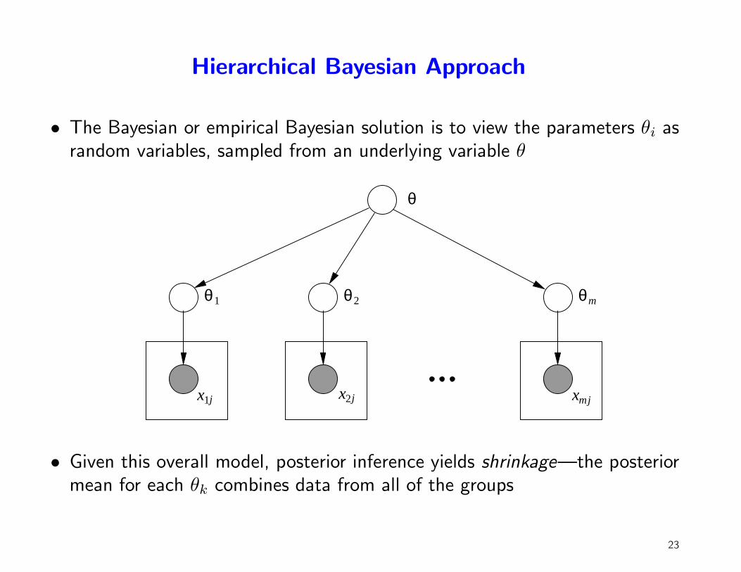
Hierarchical Bayesian Approach
• The Bayesian or empirical Bayesian solution is to view the parameters θi asrandom variables, sampled from an underlying variable θ
θ θ2 θm1
x2 xmjjx1j
θ
• Given this overall model, posterior inference yields shrinkage—the posteriormean for each θk combines data from all of the groups
23
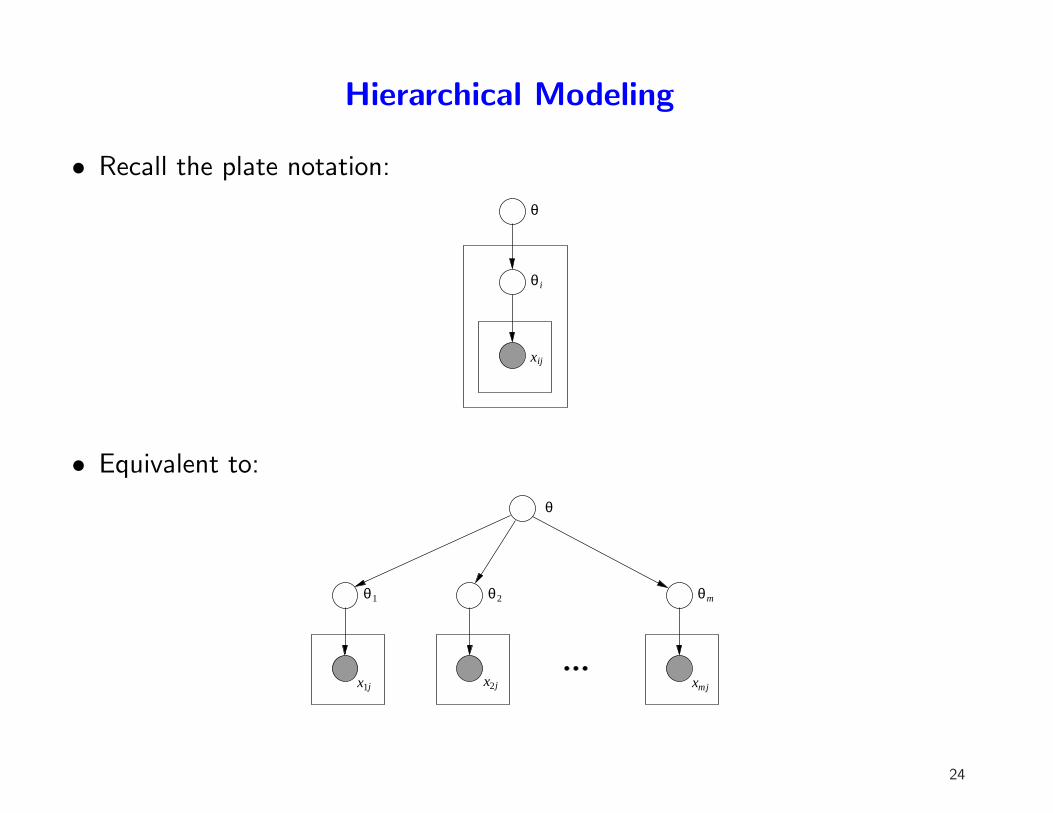
Hierarchical Modeling
• Recall the plate notation:
θ
θ i
xij
• Equivalent to:
θ θ2 θm1
x2 xmjjx1j
θ
24
Multiple Clustering Problems
• Suppose that we have M groups of data, each of which is to be clustered
• Suppose that the groups are related, so that evidence for a cluster in onegroup should be transferred to other groups
• But the groups also differ in some ways, so we shouldn’t lump the datatogether
• How do we solve the multiple group clustering problem?
• How do we solve problem when the number of clusters is unknown (withingroups and overall)?
25
Protein Folding
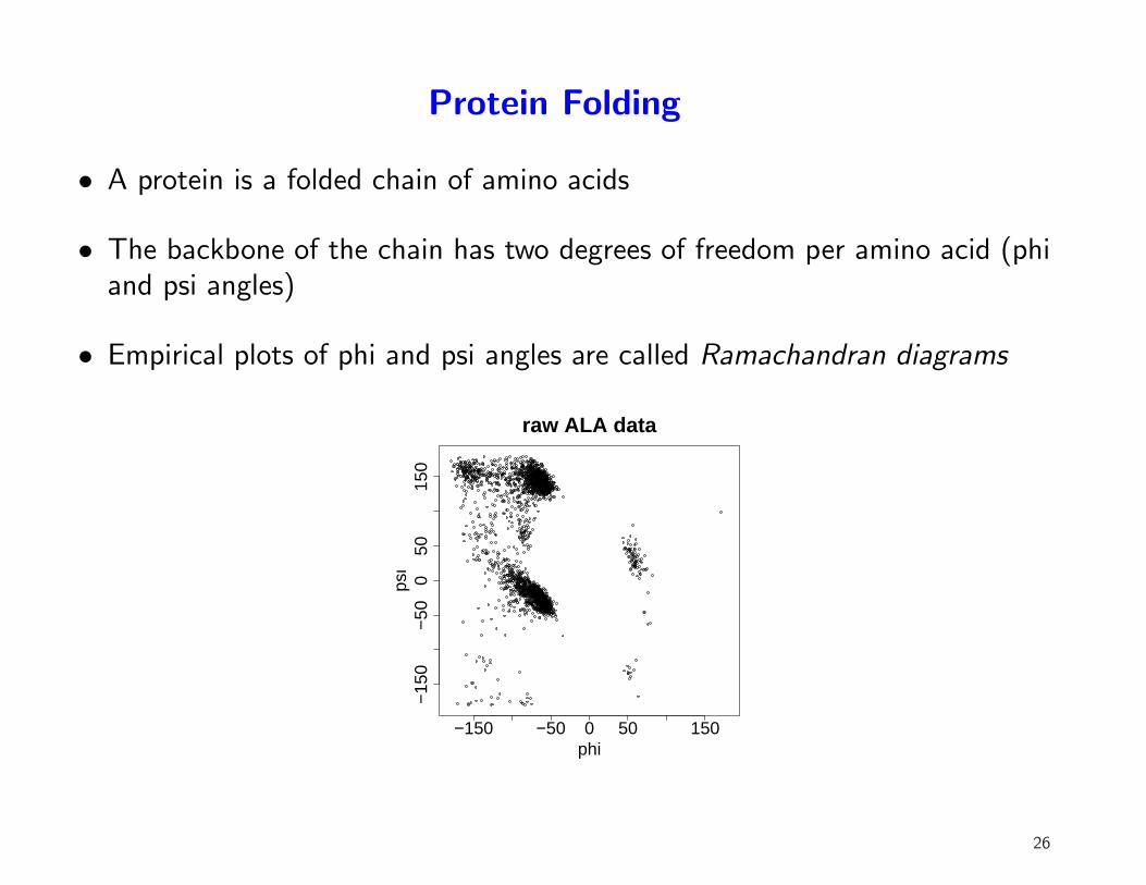
• A protein is a folded chain of amino acids
• The backbone of the chain has two degrees of freedom per amino acid (phiand psi angles)
• Empirical plots of phi and psi angles are called Ramachandran diagrams
−150 −50 0 50 150
−15
0−
500
5015
0raw ALA data
phi
psi
26
Protein Folding (cont.)
• We want to model the density in the Ramachandran diagram to provide anenergy term for protein folding algorithms
• We actually have a linked set of Ramachandran diagrams, one for eachamino acid neighborhood
• We thus have a linked set of clustering problems
– note that the data are partially exchangeable
27
Haplotype Modeling
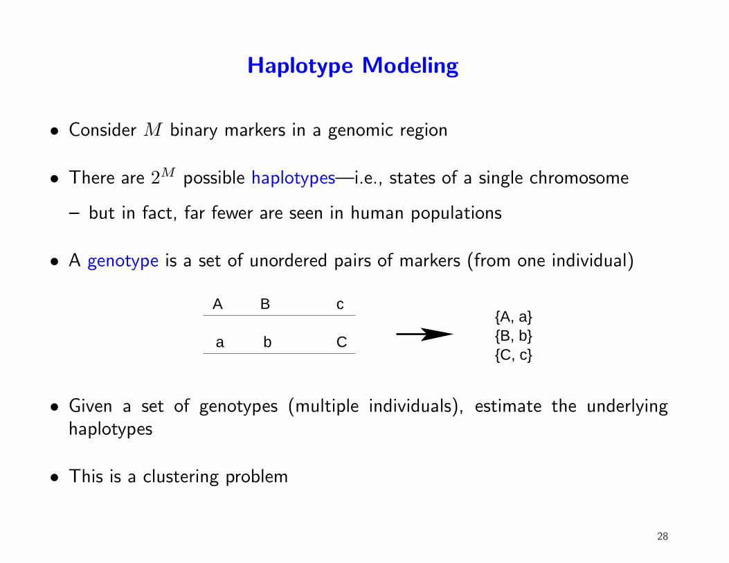
• Consider M binary markers in a genomic region
• There are 2M possible haplotypes—i.e., states of a single chromosome
– but in fact, far fewer are seen in human populations
• A genotype is a set of unordered pairs of markers (from one individual)
A B c
b Ca
{A, a}{B, b}{C, c}
• Given a set of genotypes (multiple individuals), estimate the underlyinghaplotypes
• This is a clustering problem
28
Haplotype Modeling (cont.)
• A key problem is inference for the number of clusters
• Consider now the case of multiple groups of genotype data (e.g., ethnicgroups)
• Geneticists would like to find clusters within each group but they would alsolike to share clusters between the groups
29
Natural Language Parsing
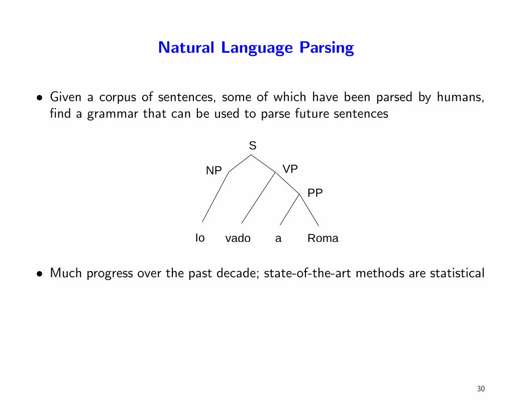
• Given a corpus of sentences, some of which have been parsed by humans,find a grammar that can be used to parse future sentences
a Romavado
S
NP VP
PP
Io
• Much progress over the past decade; state-of-the-art methods are statistical
30
Natural Language Parsing (cont.)
• Key idea: lexicalization of context-free grammars
– the grammatical rules (S → NP VP) are conditioned on the specificlexical items (words) that they derive
• This leads to huge numbers of potential rules, and (adhoc) shrinkagemethods are used to control the counts
• Need to control the numbers of clusters (model selection) in a setting inwhich many tens of thousands of clusters are needed
• Need to consider related groups of clustering problems (one group for eachgrammatical context)
31
Nonparametric Hidden Markov Models
xTx2x1
z zT2z1
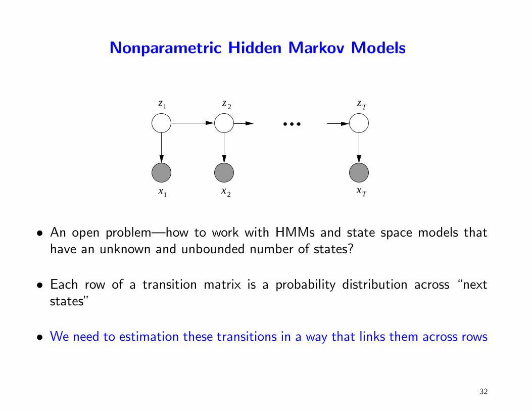
• An open problem—how to work with HMMs and state space models thathave an unknown and unbounded number of states?
• Each row of a transition matrix is a probability distribution across “nextstates”
• We need to estimation these transitions in a way that links them across rows
32
Image Segmentation
• Image segmentation can be viewed as inference over partitions
– clearly we want to be nonparametric in modeling such partitions
• Standard approach—use relatively simple (parametric) local models andrelatively complex spatial coupling
• Our approach—use a relatively rich (nonparametric) local model andrelatively simple spatial coupling
– for this to work we need to combine information across images; this bringsin the hierarchy
33
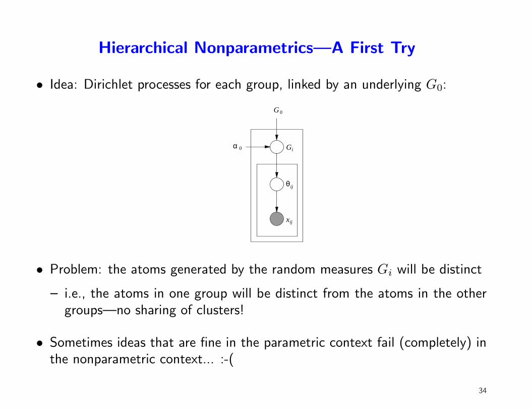
Hierarchical Nonparametrics—A First Try
• Idea: Dirichlet processes for each group, linked by an underlying G0:
x
G
ij
ij
i
θ
0α
G 0
• Problem: the atoms generated by the random measures Gi will be distinct
– i.e., the atoms in one group will be distinct from the atoms in the othergroups—no sharing of clusters!
• Sometimes ideas that are fine in the parametric context fail (completely) inthe nonparametric context... :-(
34

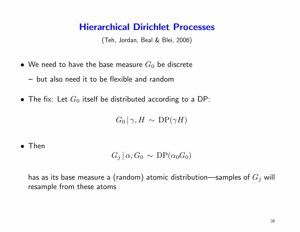
Hierarchical Dirichlet Processes
(Teh, Jordan, Beal & Blei, 2006)
• We need to have the base measure G0 be discrete
– but also need it to be flexible and random
35
Hierarchical Dirichlet Processes
(Teh, Jordan, Beal & Blei, 2006)
• We need to have the base measure G0 be discrete
– but also need it to be flexible and random
• The fix: Let G0 itself be distributed according to a DP:
G0 | γ,H ∼ DP(γH)
• ThenGj |α, G0 ∼ DP(α0G0)
has as its base measure a (random) atomic distribution—samples of Gj willresample from these atoms
36
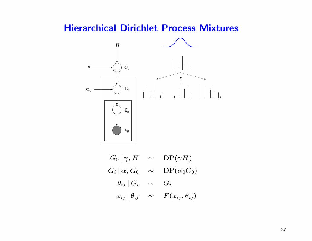
Hierarchical Dirichlet Process Mixtures
Gα 0
G0
θ
x
i
ij
ij
γ
H
G0 | γ, H ∼ DP(γH)
Gi |α, G0 ∼ DP(α0G0)
θij |Gi ∼ Gi
xij | θij ∼ F (xij, θij)
37
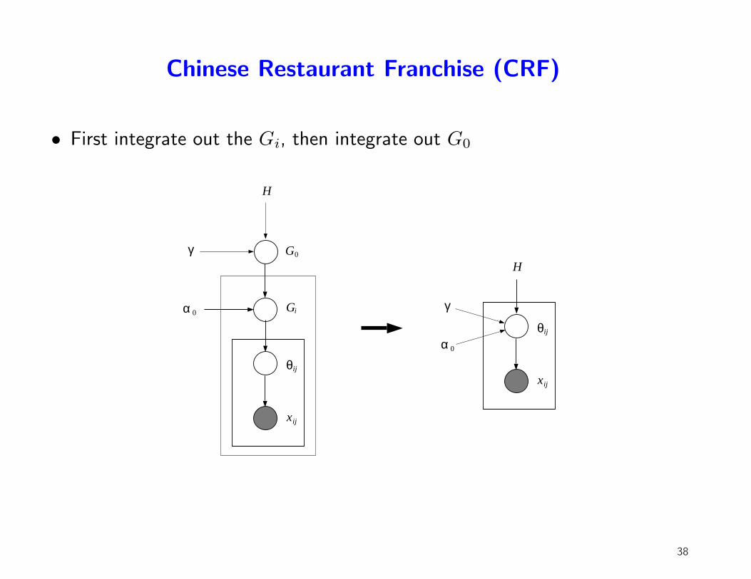
Chinese Restaurant Franchise (CRF)
• First integrate out the Gi, then integrate out G0
Gα 0
G0
θ
x
i
ij
ij
γ
H
α 0
θ
x
ij
ij
γ
H
38
Chinese Restaurant Franchise (CRF)
φ
φφ
22
21 23
24
26
25 27
28
33
34
31
32
3536
= =ψ12 =ψ
=ψ=ψ =ψ =ψ
=ψ=ψ
11 131 2 1
3 121 22 23 24
31
3 1
1 232
ψ
θθ
θ θ
θθ
θθ
θ
θ θθ
17
15
16
1211
13
1418
θθθ
θθθθθ
φ φ
φφ φ φ
φφ
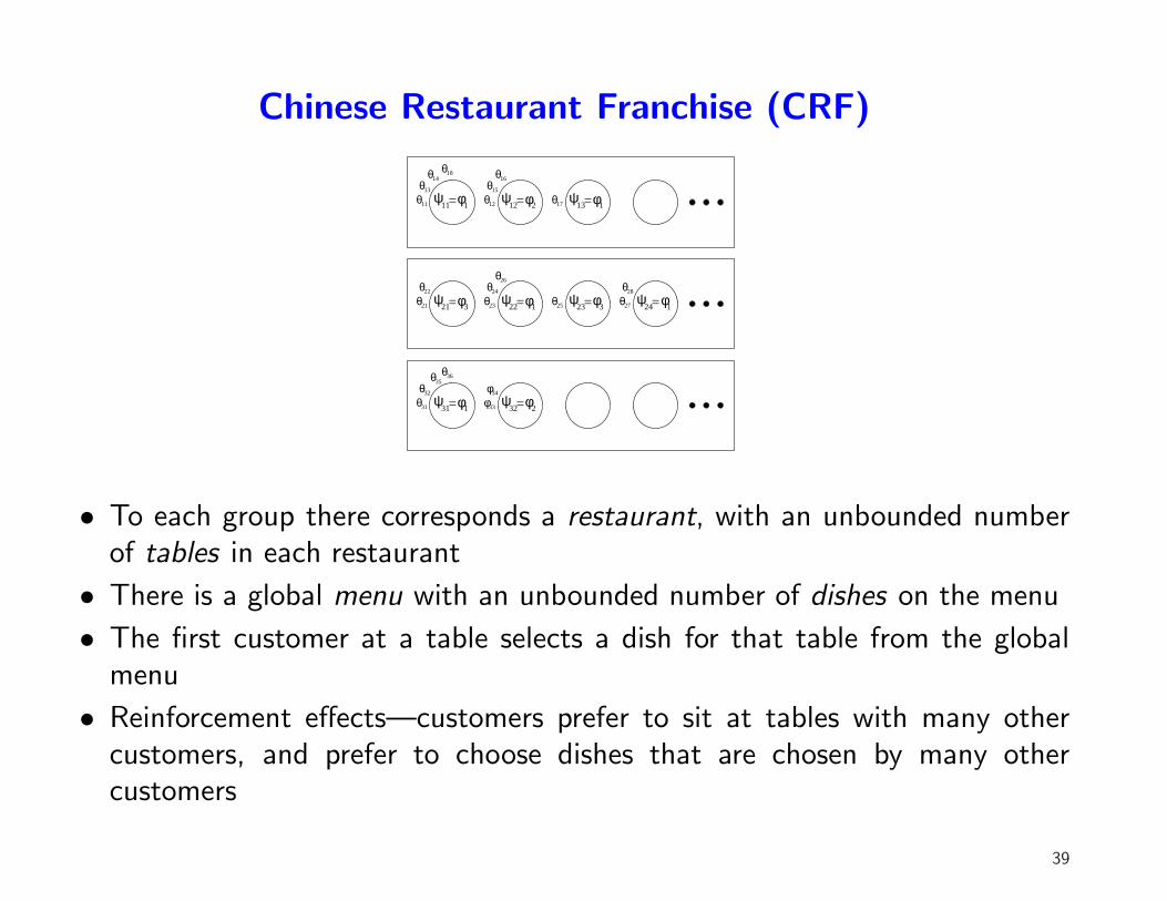
• To each group there corresponds a restaurant, with an unbounded numberof tables in each restaurant
• There is a global menu with an unbounded number of dishes on the menu
• The first customer at a table selects a dish for that table from the globalmenu
• Reinforcement effects—customers prefer to sit at tables with many othercustomers, and prefer to choose dishes that are chosen by many othercustomers
39
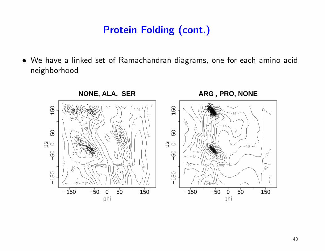
Protein Folding (cont.)
• We have a linked set of Ramachandran diagrams, one for each amino acidneighborhood
NONE, ALA, SER
phi
psi
−150 −50 0 50 150
−15
0−
500
5015
0
ARG , PRO, NONE
phi
psi
−150 −50 0 50 150
−15
0−
500
5015
0
40
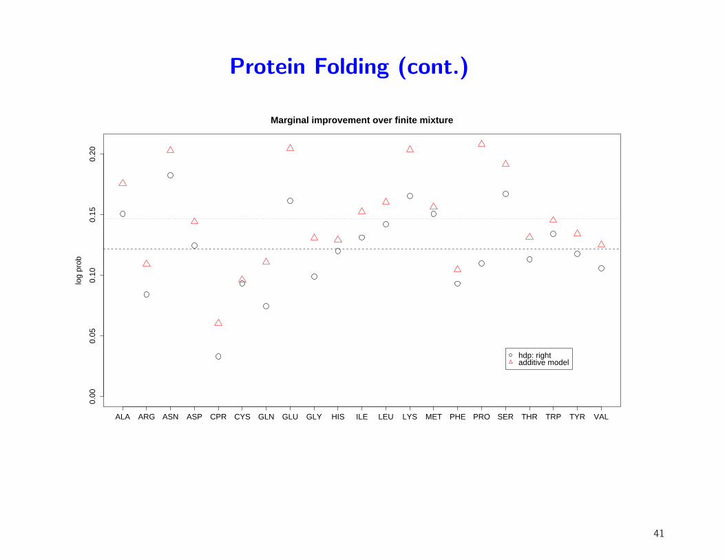
Protein Folding (cont.)
Marginal improvement over finite mixture
log
prob
0.00
0.05
0.10
0.15
0.20
ALA ARG ASN ASP CPR CYS GLN GLU GLY HIS ILE LEU LYS MET PHE PRO SER THR TRP TYR VAL
hdp: rightadditive model
41
Natural Language Parsing
• Key idea: lexicalization of context-free grammars
– the grammatical rules (S → NP VP) are conditioned on the specificlexical items (words) that they derive
• This leads to huge numbers of potential rules, and (adhoc) shrinkagemethods are used to control the choice of rules
42
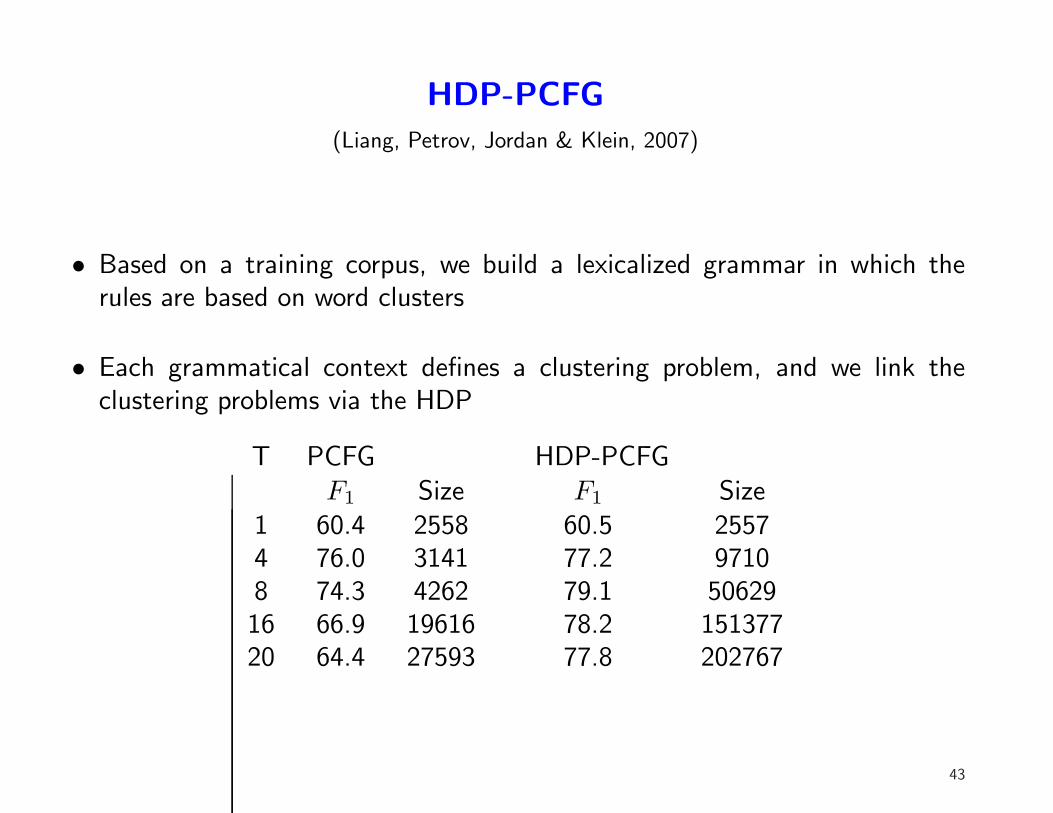
HDP-PCFG
(Liang, Petrov, Jordan & Klein, 2007)
• Based on a training corpus, we build a lexicalized grammar in which therules are based on word clusters
• Each grammatical context defines a clustering problem, and we link theclustering problems via the HDP
T PCFG HDP-PCFGF1 Size F1 Size
1 60.4 2558 60.5 25574 76.0 3141 77.2 97108 74.3 4262 79.1 5062916 66.9 19616 78.2 15137720 64.4 27593 77.8 202767
43
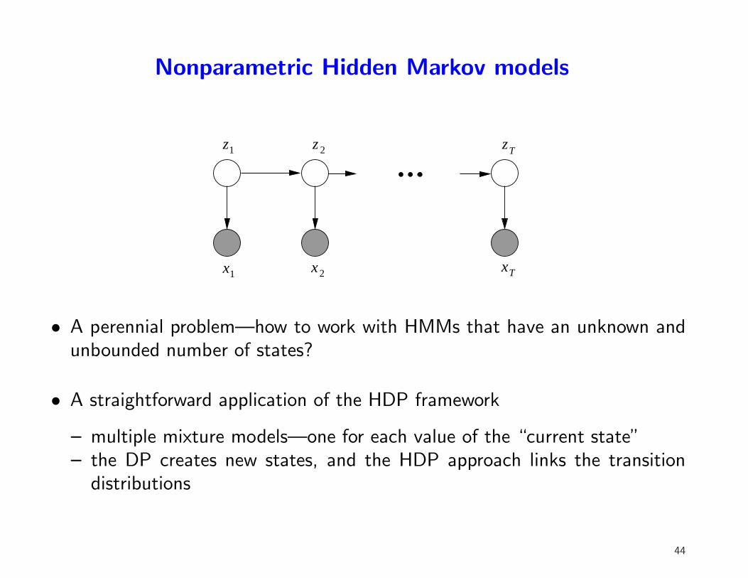
Nonparametric Hidden Markov models
xTx2x1
z zT2z1
• A perennial problem—how to work with HMMs that have an unknown andunbounded number of states?
• A straightforward application of the HDP framework
– multiple mixture models—one for each value of the “current state”– the DP creates new states, and the HDP approach links the transition
distributions
44
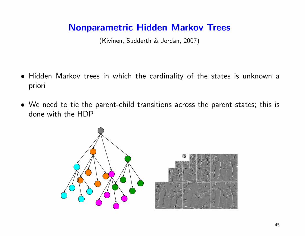
Nonparametric Hidden Markov Trees
(Kivinen, Sudderth & Jordan, 2007)
• Hidden Markov trees in which the cardinality of the states is unknown apriori
• We need to tie the parent-child transitions across the parent states; this isdone with the HDP
45
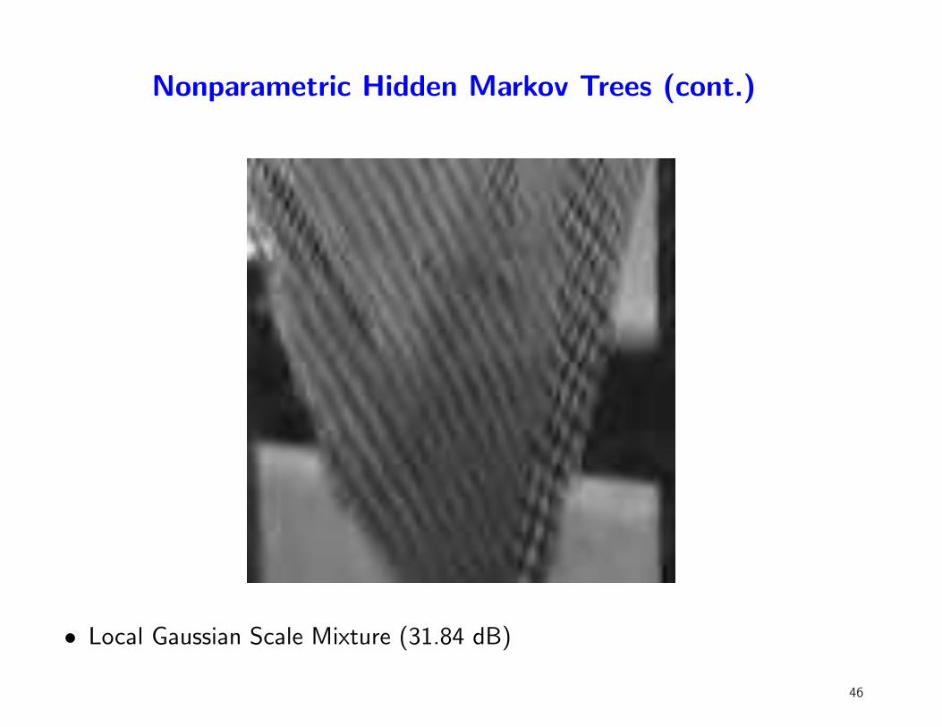
Nonparametric Hidden Markov Trees (cont.)
• Local Gaussian Scale Mixture (31.84 dB)
46
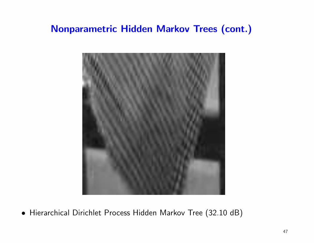
Nonparametric Hidden Markov Trees (cont.)
• Hierarchical Dirichlet Process Hidden Markov Tree (32.10 dB)
47
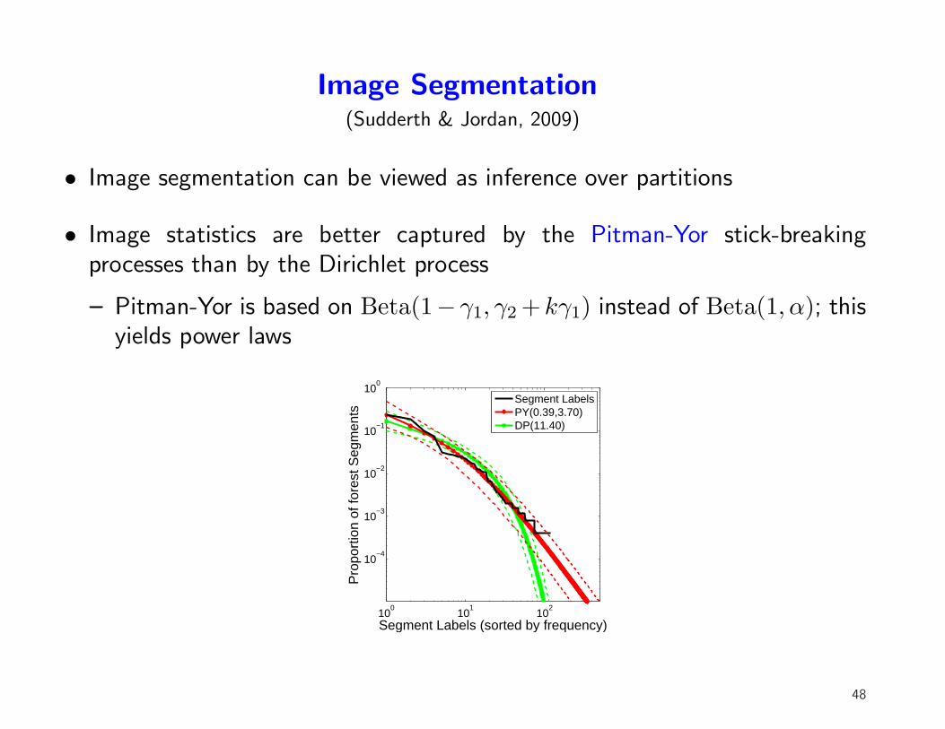
Image Segmentation(Sudderth & Jordan, 2009)
• Image segmentation can be viewed as inference over partitions
• Image statistics are better captured by the Pitman-Yor stick-breakingprocesses than by the Dirichlet process
– Pitman-Yor is based on Beta(1− γ1, γ2 + kγ1) instead of Beta(1, α); thisyields power laws
100
101
102
10−4
10−3
10−2
10−1
100
Segment Labels (sorted by frequency)
Pro
port
ion
of fo
rest
Seg
men
ts
Segment LabelsPY(0.39,3.70)DP(11.40)
48
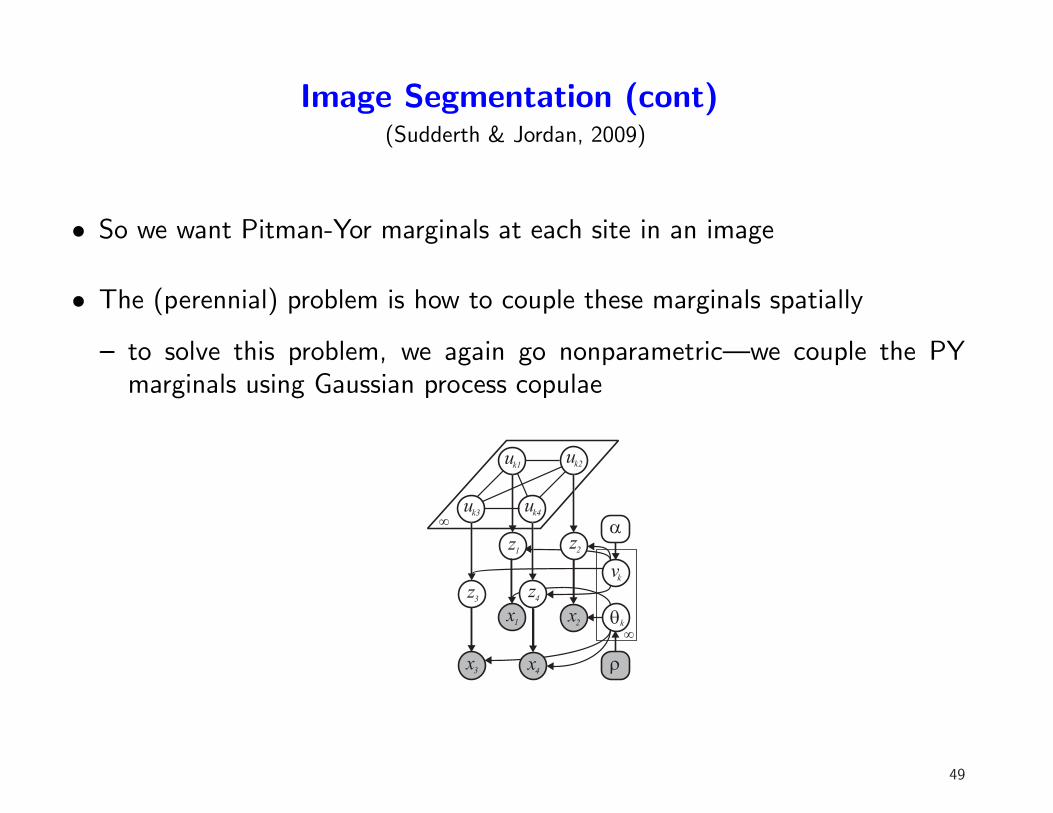
Image Segmentation (cont)(Sudderth & Jordan, 2009)
• So we want Pitman-Yor marginals at each site in an image
• The (perennial) problem is how to couple these marginals spatially
– to solve this problem, we again go nonparametric—we couple the PYmarginals using Gaussian process copulae
x1 T
D
k
f
f
U
vk
x2
x3
x4
z1
z2
z3
z4
uk3
uk4
uk1
uk2
49
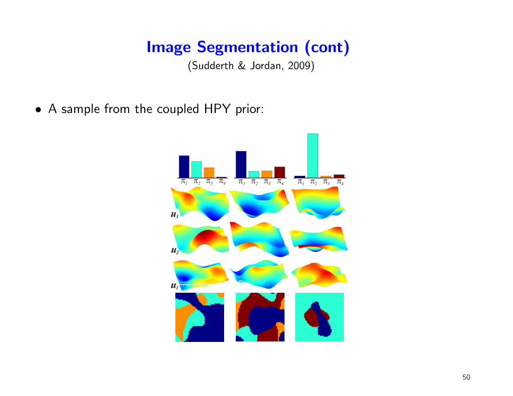
Image Segmentation (cont)(Sudderth & Jordan, 2009)
• A sample from the coupled HPY prior:
S1S2S3S4 S
1S2S3S4
u1
u2
u3
S1S2S3S4
50
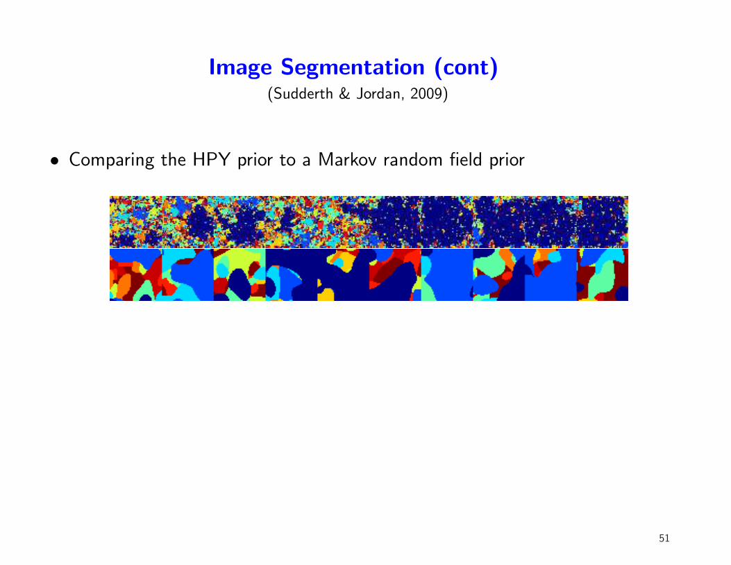
Image Segmentation (cont)(Sudderth & Jordan, 2009)
• Comparing the HPY prior to a Markov random field prior
51
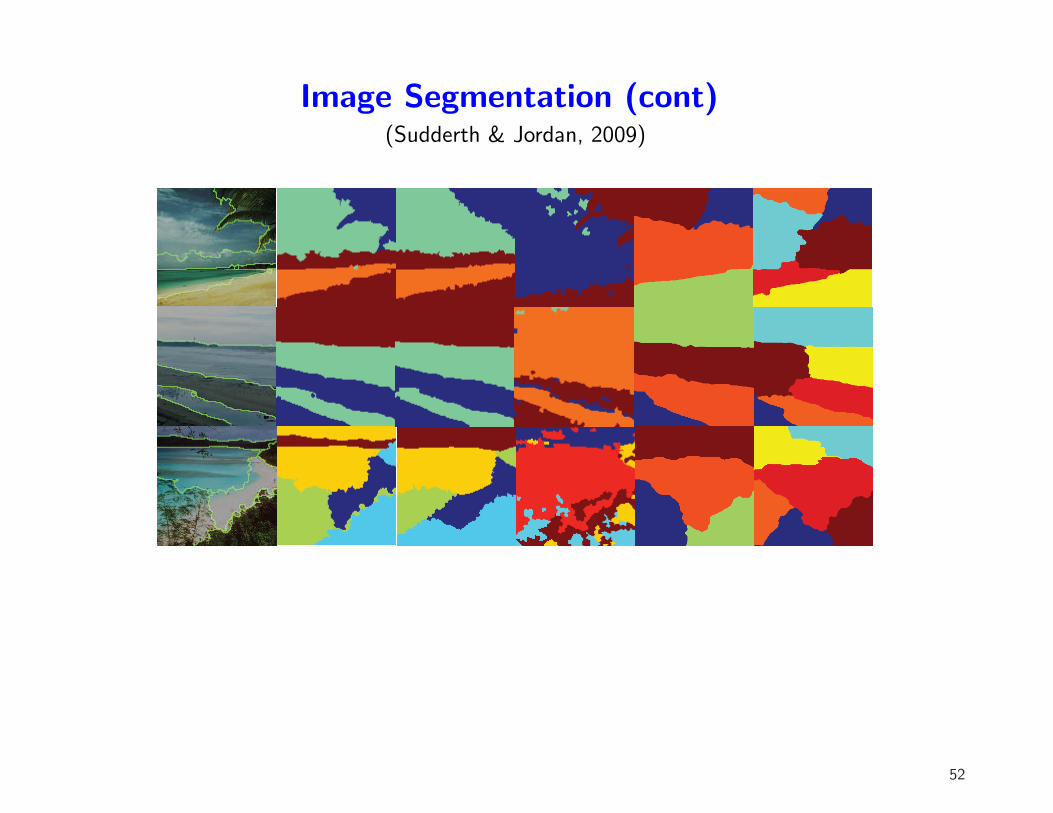
Image Segmentation (cont)(Sudderth & Jordan, 2009)
52
Beta Processes
• The Dirichlet process yields a multinomial random variable (which table isthe customer sitting at?)
• Problem: in many problem domains we have a very large (combinatorial)number of possible tables
– it becomes difficult to control this with the Dirichlet process
• What if instead we want to characterize objects as collections of attributes(“sparse features”)?
• Indeed, instead of working with the sample paths of the Dirichlet process,which sum to one, let’s instead consider a stochastic process—the betaprocess—which removes this constraint
• And then we will go on to consider hierarchical beta processes, which willallow features to be shared among multiple related objects
53
Completely random processes
• Stochastic processes with independent increments
– e.g., Gaussian increments (Brownian motion)– e.g., gamma increments (gamma processes)– in general, (limits of) compound Poisson processes
• The Dirichlet process is not a completely random processes
– but it’s a normalized gamma process
• The beta process assigns beta measure to small regions
• Can then sample to yield (sparse) collections of Bernoulli variables
54
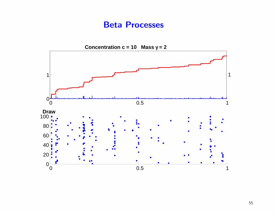
Beta Processes
0 0.5 10
1
Concentration c = 10 Mass γγγγ = 2
0 0.5 10
20
40
60
80
100Draw
1
55
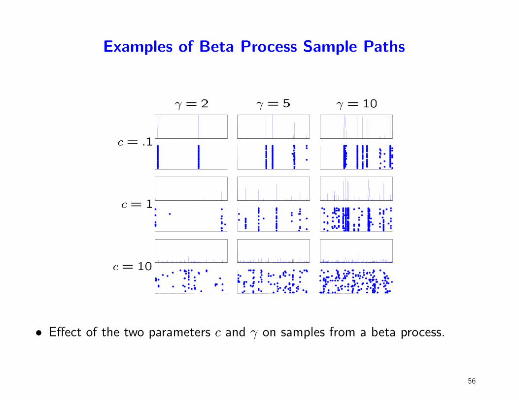
Examples of Beta Process Sample Paths
• Effect of the two parameters c and γ on samples from a beta process.
56
Beta Processes
• The marginals of the Dirichlet process are characterized by the Chineserestaurant process
• What about the beta process?
57
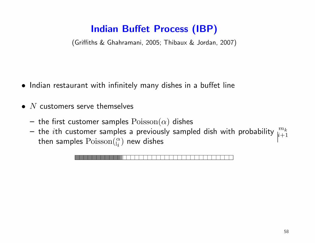
Indian Buffet Process (IBP)
(Griffiths & Ghahramani, 2005; Thibaux & Jordan, 2007)
• Indian restaurant with infinitely many dishes in a buffet line
• N customers serve themselves
– the first customer samples Poisson(α) dishes– the ith customer samples a previously sampled dish with probability mk
i+1then samples Poisson(α
i) new dishes
58
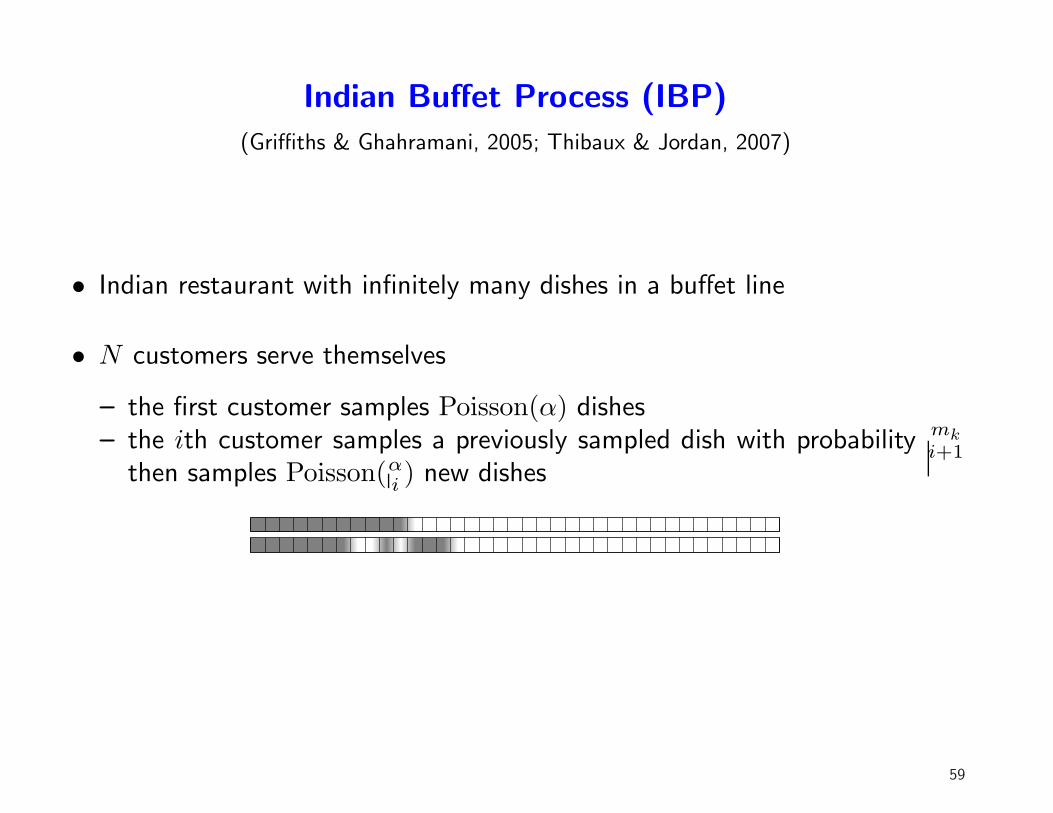
Indian Buffet Process (IBP)
(Griffiths & Ghahramani, 2005; Thibaux & Jordan, 2007)
• Indian restaurant with infinitely many dishes in a buffet line
• N customers serve themselves
– the first customer samples Poisson(α) dishes– the ith customer samples a previously sampled dish with probability mk
i+1then samples Poisson(α
i) new dishes
59
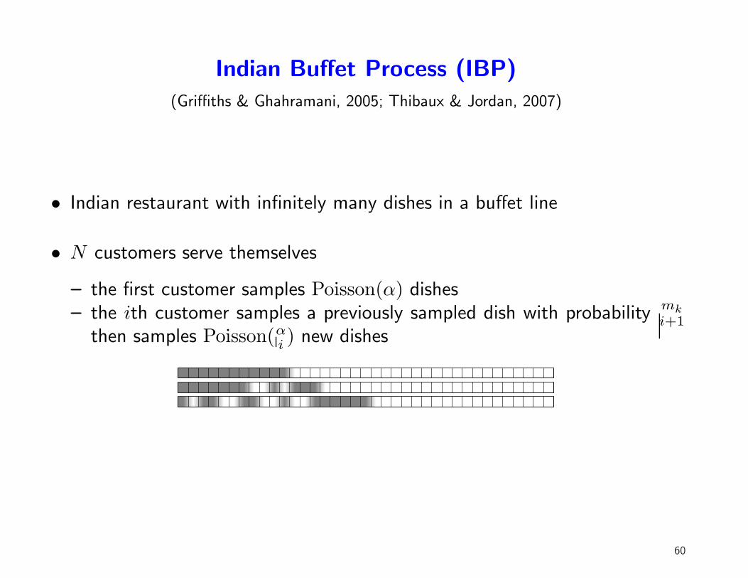
Indian Buffet Process (IBP)
(Griffiths & Ghahramani, 2005; Thibaux & Jordan, 2007)
• Indian restaurant with infinitely many dishes in a buffet line
• N customers serve themselves
– the first customer samples Poisson(α) dishes– the ith customer samples a previously sampled dish with probability mk
i+1then samples Poisson(α
i) new dishes
60
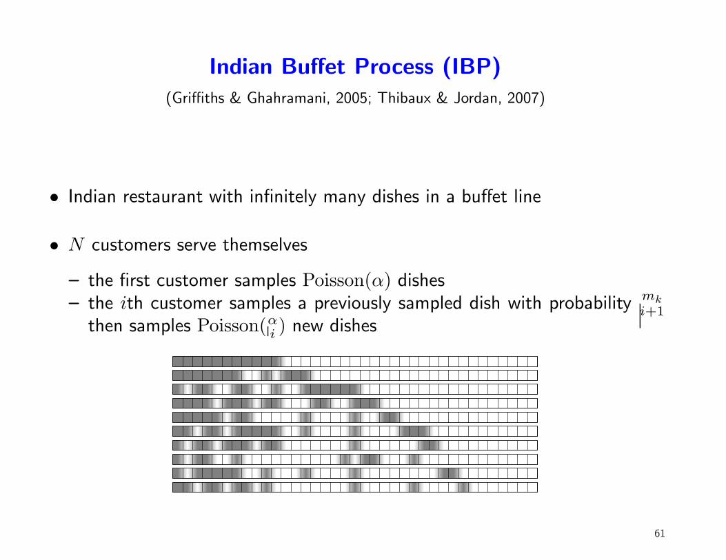
Indian Buffet Process (IBP)
(Griffiths & Ghahramani, 2005; Thibaux & Jordan, 2007)
• Indian restaurant with infinitely many dishes in a buffet line
• N customers serve themselves
– the first customer samples Poisson(α) dishes– the ith customer samples a previously sampled dish with probability mk
i+1then samples Poisson(α
i) new dishes
61
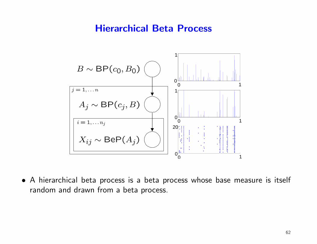
Hierarchical Beta Process
0 10
1
0 10
1
0 10
20
• A hierarchical beta process is a beta process whose base measure is itselfrandom and drawn from a beta process.
62
Conclusions
• Nonparametric Bayesian modeling: flexible data structures meet probabilisticinference
• The underlying theory has to do with exchangeability and partialexchangeability
• We haven’t discussed inference algorithms, but many interesting issues andnew challenges arise
• For more details, including tutorials:
http://www.cs.berkeley.edu/∼jordan
63