Applied Soft Computing - Amirkabir University of Technologyce.aut.ac.ir/~meybodi/paper/Sharifi-ff-Kazemi-Mahdavian-meybodi... · A. Shariﬁ et al. / Applied Soft Computing 32 (2015)

Asp

AMa

4b

a

ARRAA

KDMDMPN

1

irrlmwci

jm(

h1

Applied Soft Computing 32 (2015) 432–448

Contents lists available at ScienceDirect

Applied Soft Computing

j ourna l ho me page: www.elsev ier .com/ locate /asoc

novel hybrid adaptive collaborative approach based on particlewarm optimization and local search for dynamic optimizationroblems

li Sharifia, Javidan Kazemi Kordestanib,∗, Mahshid Mahdaviania,ohammad Reza Meybodia

Soft Computing Laboratory, Computer Engineering and Information Technology Department, Amirkabir University of Technology (Tehran Polytechnic),24 Hafez Ave., Tehran, IranDepartment of Computer Engineering, Science and Research Branch, Islamic Azad University, Tehran, Iran

r t i c l e i n f o

rticle history:eceived 6 August 2014eceived in revised form 1 January 2015ccepted 2 April 2015vailable online 13 April 2015

eywords:ynamic optimization problemsoving peaks benchmarkOPsPB

article swarm optimizer

a b s t r a c t

This paper proposes a novel hybrid approach based on particle swarm optimization and local search,named PSOLS, for dynamic optimization problems. In the proposed approach, a swarm of particles withfuzzy social-only model is frequently applied to estimate the location of the peaks in the problem land-scape. Upon convergence of the swarm to previously undetected positions in the search space, a localsearch agent (LSA) is created to exploit the respective region. Moreover, a density control mechanismis introduced to prevent too many LSAs crowding in the search space. Three adaptations to the basicapproach are then proposed to manage the function evaluations in the way that are mostly allocatedto the most promising areas of the search space. The first adapted algorithm, called HPSOLS, is aimedat improving PSOLS by stopping the local search in LSAs that are not contributing much to the searchprocess. The second adapted, algorithm called CPSOLS, is a competitive algorithm which allocates extrafunction evaluations to the best performing LSA. The third adapted algorithm, called CHPSOLS, combines

aive direct search the fundamental ideas of HPSOLS and CPSOLS in a single algorithm. An extensive set of experiments isconducted on a variety of dynamic environments, generated by the moving peaks benchmark, to evaluatethe performance of the proposed approach. Results are also compared with those of other state-of-the-art algorithms from the literature. The experimental results indicate the superiority of the proposedapproach.

© 2015 Elsevier B.V. All rights reserved.

. Introduction

Optimization in dynamic environments has emerged as anmportant field of research during the last two decades, since manyeal-world optimization problems tend to change over time. Theepresentative examples of real-world dynamic optimization prob-ems (DOPs) are portfolio decisions optimization in changing stock

arket conditions, shortest path routing problem in changing net-
ork environments, and vehicle routing with online arrival of
ustomer’s requests. In these problems, the task of optimizations not confined to finding the optimum solution(s) in the problem

∗ Corresponding author. Tel.: +98 9373908326.E-mail addresses: [email protected] (A. Sharifi),

[email protected] (J. Kazemi Kordestani),[email protected] (M. Mahdaviani), [email protected]

M.R. Meybodi).

ttp://dx.doi.org/10.1016/j.asoc.2015.04.001568-4946/© 2015 Elsevier B.V. All rights reserved.

space but to continuously and accurately adapt to the new condi-tions during the course of optimization.

Each dynamic optimization problem P can be defined by a quin-tuple {˝, x, �, f, t} where ̋ denotes the search space, x is a feasiblesolution in ˝, � represents the system control parameters whichdetermines the distribution of the solutions in the fitness land-scape, f is the static objective function and t is the time. P is thencan be modeled as follows [1]:

P =∑end

t=0ft(x, �) (1)

As can be seen in the above equation, dynamic optimization prob-
lem P is composed of a sequence of static instances. Hence, the goalof the optimization in such problems is no longer just locating theoptimal solution(s), but rather tracking the shifting optima over thetime.
dx.doi.org/10.1016/j.asoc.2015.04.001

http://www.sciencedirect.com/science/journal/15684946

www.elsevier.com/locate/asoc

http://crossmark.crossref.org/dialog/?doi=10.1016/j.asoc.2015.04.001&domain=pdf

mailto:[email protected]




dx.doi.org/10.1016/j.asoc.2015.04.001

ft Com

t

�

wrTs

f

[sra

iiaintCol

qtum

aaocapa

oeiia

A. Sharifi et al. / Applied So

The dynamism of the problem can then be obtained by tuninghe system control parameters as follows:

t+1 = �t ⊕ �� (2)

here �� is the deviation of the control parameters from their cur-ent values and ⊕ represents the way the parameters are changed.he next state of the environment then can be defined using currenttate of the environment as follows:

t+1(x, �) = ft(x, �t ⊕ ��) (3)

Different change types can be defined, using �� and ⊕. Li et al.1] proposed a framework of the eight change types including smalltep change, large step change, random change, chaotic change, recur-ent change, recurrent change with noise, and dimensional change. Fordditional information, interested readers are referred to [1].

The adaptive nature of evolutionary algorithms and swarmntelligence methods make them suitable candidates for deal-ng with DOPs. However, the dynamic behavior of DOPs posesdditional challenges to the evolutionary algorithms and swarmntelligence techniques. The main challenge of the mentioned tech-iques in dynamic environments is diversity loss which arises dueo the tendency of the population to converge to a single optimum.onsequently, when a change occurs in environment, the numberf function evaluations required for a partially converged popu-ation to re-diversify and re-converge to the shifted optimum is

uite deleterious to the performance [2]. Particle swarm optimiza-ion (PSO) is one of the swarm intelligence algorithms that shouldndergo a certain adjustment to work well in dynamic environ-ents.In this paper, a novel PSO-based approach which combines

fuzzy social-only model PSO and local search is suggested toddress DOPs. The basic algorithm is then further extended basedn three resource management schemes. Experimental studies arearried out on the sensitivity analysis of the several componentsnd parameters of the proposed method. The performance of theroposed approach is also compared with several state-of-the-artlgorithms on moving peaks benchmark (MPB) problem.

The rest of this paper is structured as follows: Section 2 gives anverview to the basic PSO algorithm and its variants for dynamic
nvironments. In Section 3, we explain our proposed approachn detail. Experimental study regarding the parameters sensitiv-ty analysis, impact of using different local search methods, effect ofpplying different resource management schemes, and comparison
puting 32 (2015) 432–448 433

with other state-of-the-art methods is presented in Section 4.Finally, conclusions and future works are given in Section 5.

2. Background and related works

PSO is a versatile population-based stochastic optimizationmethod which was first proposed by Kennedy and Eberhart [3] in1995. PSO begins with a population of randomly generated parti-cles in a D-dimensional search space. Each particle i of the swarmhas three features: �xi that shows the current position of the particlei in the search space, �vi which is the velocity of the particle i and �pi

which denotes the best position found so far by the particle i. Eachparticle i updates its position in the search space, at every time stept, according to the following equations:

�vi(t + 1) = w�vi(t) + c1r1[�pi(t) − �xi(t)] + c2r2[�pg(t) − �xi(t)] (4)

�xi(t + 1) = �xi(t) + �vi(t + 1) (5)

where w is the inertia weight parameter which determines theportion of velocity preserved during the last time step of the algo-rithm. c1 and c2 denote the cognitive and social learning factorsthat are used to adjust the degree of the movement of particlestoward their personal best position and global best position of theswarm, respectively. r1 and r2 are two independent random vari-ables drawn with uniform probability from [0,1]. Finally, �pg is theglobally best position found so far by the swarm. The pseudo-codeof the PSO is shown in Algorithm 1.

PSO has been successfully applied in many optimization prob-lems including numerical optimization [4,5], image processing [6],training feedforward neural networks in dynamic environments[7], density estimation [8], multi-objective optimization [9,10],data clustering [11], etc. However, as we mentioned in Section1, PSO suffers from diversity loss when dealing with DOPs. Manyattempts have been made by the researchers to deal with this issue.In the rest of this section, we will examine the current studies andadvances in the literature in five major groups.

2.1. Injecting diversity to the swarm after detecting a change inthe environment

A very basic strategy to cope with diversity loss problem is toinject a certain level of diversity to the swarm whenever a changeoccurs in the environment. An example of this approach is the re-
randomization PSO (RPSO) proposed by Hu and Eberhart [12]. InRPSO, upon detecting a change in the environment, the entire or apart of the swarm is randomly relocated in the search space. Theirresults suggest that the re-randomization of a small portion of the

4 ft Com

siethmoeo

2

dv

2

ttamtp

2

sptbsaucwenn

2

oLsa

2

ttpeicpathtmfii

34 A. Sharifi et al. / Applied So

warm (i.e. 10% in their study) can improve the ability of the canon-cal PSO in tracking the shifting optimum, when the step size of thenvironmental change is small. It should be noted that specifyinghe proper rate of randomization is a challenging task. One the oneand, too much randomization will result in losing too much infor-ation and resemble solving the problem from scratch. One the

ther hand, too little randomization might be unable to introducenough diversity to the swarm, which is necessary for tracking theptimum.

.2. Maintaining diversity throughout the run

A group of studies have tried to preserve a sustainable level ofiversity during the entire run by avoiding individuals from con-erging to a single optimum.

.2.1. Mutual repulsionApplying a mutual repulsion between particles, swarms or cap-

ured optimums can maintain a suitable level of diversity duringhe search process. The atomic model [13,14] used in mCPSO isn example of utilizing repulsion for dynamic environments. InCPSO, each swarm contains a number of charged classical par-

icles. Charged classical particles in each swarm repel each other torovide a sustainable diversity among the individuals.

.2.2. Dynamic information topologySome researchers have modified the topology of information

haring among the particles of the swarm in order to improve theerformance of PSO in dealing with dynamic situations. This canemporarily reduce the tendency of particles to move toward theest found positions, thereby enhancing the diversity among thewarm. For example, Janson and Middendorf [15] studied a hier-rchical PSO (H-PSO) for noisy and dynamic environments. H-PSOses a tree-like structure to establish a hierarchy between parti-les. They also proposed a partitioned hierarchical PSO (PH-PSO)here the tree is temporarily partitioned into sub-swarms after an

nvironmental change is detected. Both approaches reported a sig-ificant improvement over standard PSO on different dynamic andoisy functions.

.2.3. OthersBeside the above strategies, some researchers have considered

ther types of techniques to maintain diversity throughout the run.i and Yang [16], for example, incorporated a random immigrantscheme into PSO where a temporal population is randomly gener-ted if the population diversity drops below a constant threshold.

.3. Memory-based approaches

Many studies have proved that making use of a memory schemeo restore useful information about previously found positions inhe search space can be beneficial for various DOPs. For exam-le, Wang et al. [17] proposed a memory-based PSO for dynamicnvironments. In this method, the entire population is dividednto three parts: (1) “explore”-population which is responsible forollecting information about the good solutions, (2) “memory”-opulation for storing and retrieving information about promisingreas of the search space, and (3) “exploit”-population that is usedo refine the solutions around the areas provided by memory. Theyave introduced two new operators called memory-based reset-
ing and memory-based immigrants to transfer information from
emory to “exploit”-population. Their experimental results con-rm that the memory scheme can enhance the performance of PSO

n dynamic environments.

puting 32 (2015) 432–448

2.4. Multi-swarm PSO

The most widely used technique to cope with diversity loss prob-lem is to make use of multiple swarms or to divide the particles ofthe main swarm into several sub-swarms, and assign them to dif-ferent areas of the search space. In the rest of this sub-section, weexamine two major types of multi-swarm PSOs for DOPs.

2.4.1. Methods with a fix number of swarmsVarious methods exist in the literature that have used a fixed

number of swarms to capture several promising areas of the searchspace in parallel. The pioneer work in this context was done byBlackwell and Branke [18]. They introduced a multi-swarm algo-rithm based on the atomic metaphor, namely mQSO. The mQSOstarts with a predefined number of swarms, typically equal to thenumber of peaks in the landscape, exploring in the search space tolocate the optima. In mQSO, each swarm is composed of a num-ber of neutral particles and a number of quantum particles. Neutralparticles update their velocity and position according to the prin-ciples of pure PSO. On the other hand, quantum particles do notmove according to the PSO dynamics but change their positionsaround the center of the best particle of the swarm according to arandom uniform distribution with radius rcloud. Consequently, theynever converge, but provide the swarm with a sustainable levelof diversity needed for tracking the shifting optimum. They alsointroduced two operators to establish two forms of interactionsbetween swarms. First operator named exclusion, which preventspopulations from settling on the same peak by reinitializing theworst performing swarm in the search space. Second operator isreferred to as anti-convergence which is triggered whenever allswarms converge, and removes the worst swarm from its peakand reinitializes it in the search space. These two operators haveinitiated two implications for other researchers as: (a) search oftwo populations in the same area is not efficient and (b) it is nec-essary for different methods to be able to detect new emergingpeaks, specifically in the environments with an unknown numberof peaks.

2.4.2. Methods with varying number of swarms2.4.2.1. Use of adaptation mechanisms for determining the number ofpopulations. The critical drawback of the multi-swarm algorithmproposed in [18] is that the number of swarms should be definedbefore the optimization process, whereas in real-world problemsthe information about the environment may not be in hand. Thevery first attempt to adapt the number of swarms in dynamic envi-ronments was made by Blackwell [2]. He introduced self-adaptiveversion of mQSO, which dynamically adjusts the number of swarmseither by spawning new swarms into the search space, or bydestroying redundant swarms [2]. In this algorithm, swarms arecategorized into two groups: free swarms, whose expansion, i.e.the maximum distance between any two particles in the swarm inall dimensions, are larger than radius rconv, and converged swarms.Once the expansion of a free swarm, becomes smaller than a radiusrconv, it is converted to the converged swarm. In AmQSO, when thenumber of free swarms (Mfree) is dropped to zero, a free swarm isinitialized in the search space for capturing undetected peaks. Onthe other hand, free swarms are removed from the search space ifMfree is higher than a threshold nexcess.

2.4.2.2. Clustering the main swarm into some sub-swarms. Dividingthe main population of the algorithm into several clusters, i.e. sub-populations, via clustering methods and assigning each of them to
different promising regions of the search space is a relatively newmulti-population scheme for DOPs which has shown promisingresults [19]. For example, Parrott and Li [20] proposed a Speciation-based Particle Swarm Optimization (SPSO) for tracking multiple

ft Com

ops

taEmccpitewwi

scaaserusc

2asvaisTirsmcfsttcto

ettilpbbM

2Tieie


ptima in dynamic environments, which dynamically distributesarticles of the main swarm over a variable number of so-calledpecies.

Yang and Li [21] employed a single linkage hierarchical clus-ering method to create an adaptive number of sub-swarms, andssign them to different promising sub-regions of the search space.ach created sub-swarm then uses the PSO with a modified gbestodel to exploit the respective region. In order to avoid different

lusters from crowding, they have applied a redundancy controlheck. In this regard, when two sub-swarms are located on a singleeak, first they are merged together and then the worst perform-

ng individuals of the sub-swarm are removed until its size is equalo a predefined threshold. In another work [16], they have furtherxtended the fundamental idea of CPSO and introduced a frame-ork for multi-population methods in undetectable environments,here the detection of environmental changes is very difficult or

mpossible.Nickabadi et al. [22] proposed a competitive clustering particle

warm optimizer (CCPSO) for DOPs. They employed a multi-stagelustering procedure to split the particles of the main swarm over

varying number of sub-swarms based on the particles positionss well as their objective function values. In addition to the sub-warms, there is also a group of free particles that explore thenvironment to locate new emerging optima or exploit the cur-ent optima which are not followed by any sub-swarm, and arepdated using a cognitive-only movement model. Moreover, eachub-swarm adjusts its inertia weight according to the success per-entage of the sub-swarm [23].

.4.2.3. Multi-swarm scheme based on space partitioning. Anotherpproach for dealing with diversity loss problem is to divide theearch space into several partitions and keep the number of indi-iduals in each partition less than a predefined threshold. Hashemind Meybodi [24] incorporated PSO and Cellular Automata (CA)nto an algorithm referred to as cellular PSO. In cellular PSO, theearch space is partitioned into some equally sized cells using CA.hen, particles of the swarm are allocated to different cells accord-ng to their positions in the search space. At any time, particlesesiding in each cell use their personal best experience and the bestolution found in their neighborhood cells for searching an opti-um. Moreover, whenever the number of particles within each

ell exceeds a predefined threshold, randomly selected particlesrom the saturated cells are transferred to random cells within theearch space. In addition, each cell has a memory that is used to keeprack of the best position found within the boundary of the cell andhe best position among its neighbors. In another work [25], theyhanged the role of some particles in each cell, from standard par-icles to quantum particles for a few iterations upon the detectionf a change in the environment.

With the aim to improve the performance of cellular PSO, Sharifit al. [26] proposed a two phased collaborative algorithm, namedwo phased cellular PSO (TP-CPSO). In TP-CPSO, each cell can func-ion in two different phases: exploration phase, in which the searchs performed by a modified PSO algorithm until a convergence toocal optima is detected, and exploitation phase, in which the searchrocess is conducted by a directed local search with a high capa-ility of exploitation. Initially, all cells are in exploration phase,ut upon converging to local optima they go to exploitation phase.oreover, they eliminated the need for defining a limit for each cell.

.4.2.4. Methods with a parent swarm and various child swarms.he major strategy in this approach is to divide the search space
nto different sub-regions, using a parent swarm, and carefullyxploit each sub-region with a distinct child swarm. Several stud-es exist in the literature that have followed this approach. Forxample, Kamosi et al. [27] introduced a multi-swarm algorithm
puting 32 (2015) 432–448 435

for dynamic environments, which consists of a parent swarm toexplore the search space and a varying number of child swarms toexploit promising areas found by the parent swarm. In this method,called mPSO, the optimization process starts with a parent swarmexploring the entire search space for locating promising areas ofthe search space. Whenever the fitness value of the best parti-cle in the parent swarm improves, a child swarm will be createdas follows: (a) a number of particles located within the radius rfrom the best particle of the parent swarm are separated from theparent swarm and form a new child swarm and (b) a number ofparticles are randomly initialized in a hyper-sphere with radiusr/3 centered at the best particle of the child swarm. Afterwards, anumber of randomly initialized particles are added to the parentswarm in order to compensate for the migration of particles fromparent swarm to the child swarm. After creating child swarms, eachof them exploits their respective sub-regions in the search space.Upon detecting a collision between two child swarms, the worsechild swarm is removed. In case that a particle of the parent swarmfinds a better position in the search territory of a child swarm, itreplaces the local best particle of the respective child swarm. After-wards, the particle of the parent swarm is reinitialized in the searchspace. In another work, inspired by hibernation phenomenon inanimals, they extended mPSO and proposed a hibernating multi-swarm algorithm (HmSO) [28]. In HmSO, unproductive search inchild swarms is stopped by “sleeping” converged child swarms. Thishibernation mechanism makes more function evaluations availablefor the parent swarm to explore the search space, and for the otherchild swarms to exploit their respective areas in the landscape.

Recently, Yazdani et al. [29] employed several mechanisms ina multi-swarm algorithm to conquer the existing challenges indynamic environments. In their proposed method, named FTMPSO,a randomly initialized finder swarm exploring the entire searchspace for locating the position of the peaks. Upon convergenceof the finder swarm, a tracker swarm will be activated by trans-ferring the fittest particles from the finder swarm into the newlycreated tracker swarm. The finder swarm is then reinitialized intothe search space to capture other uncovered peaks. Afterwards,the activated tracker swarm is responsible for finding the top ofthe peak using a local search along with following the respec-tive peak upon detecting a change in the environment. In order toavoid tracker swarms exploiting the same peak, exclusion is appliedbetween every pair of tracker swarms. Besides, if the finder swarmconverges to a populated peak, it is reinitialized into the searchspace without generating any tracker swarm.

Our proposed approach is relatively similar to the methods ofthis group in the sense that it uses a main swarm to explore thesearch space. However, instead of using child swarms for explo-iting promising areas of the search space, in this work we applylocal search agents. Moreover, we use various schemes to effec-tively allocate the function evaluations to the most promising areasof the search space.

2.5. PSO with adaptive scheme

In this approach, knowledge on the search process from differ-ent particles is included to improve the efficiency and effectivenessof the search process. Moreover, in this approach, different schemesand operators are further devised to promote the ability of theparticles to deal with the environmental dynamism. For example,inspired by composite particles in physic, Liu et al. [30] introduceda new variant of PSO, called PSO with composite particles (PSO-CP)for DOPs. PSO-CP contains four major components: (1) compos-
ite particles which are formed by iteratively grouping the worstparticles with two of their nearest particles, (2) scattering opera-tor which aims at enhancing the local diversity within compositeparticles, (3) velocity-anisotropic reflection scheme that can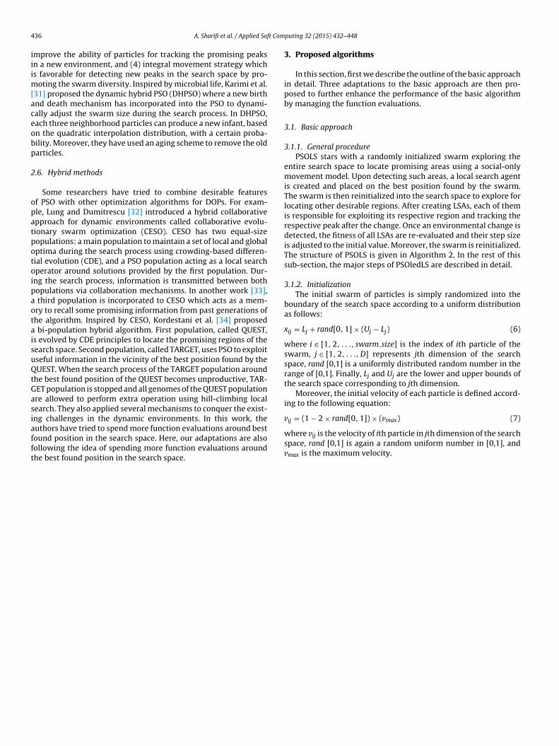

4 ft Com

iiim[aceobp

2

opatpotoipaotaisuQtGasiafft

ij max


mprove the ability of particles for tracking the promising peaksn a new environment, and (4) integral movement strategy whichs favorable for detecting new peaks in the search space by pro-

oting the swarm diversity. Inspired by microbial life, Karimi et al.31] proposed the dynamic hybrid PSO (DHPSO) where a new birthnd death mechanism has incorporated into the PSO to dynami-ally adjust the swarm size during the search process. In DHPSO,ach three neighborhood particles can produce a new infant, basedn the quadratic interpolation distribution, with a certain proba-ility. Moreover, they have used an aging scheme to remove the oldarticles.

.6. Hybrid methods

Some researchers have tried to combine desirable featuresf PSO with other optimization algorithms for DOPs. For exam-le, Lung and Dumitrescu [32] introduced a hybrid collaborativepproach for dynamic environments called collaborative evolu-ionary swarm optimization (CESO). CESO has two equal-sizeopulations: a main population to maintain a set of local and globalptima during the search process using crowding-based differen-ial evolution (CDE), and a PSO population acting as a local searchperator around solutions provided by the first population. Dur-ng the search process, information is transmitted between bothopulations via collaboration mechanisms. In another work [33],

third population is incorporated to CESO which acts as a mem-ry to recall some promising information from past generations ofhe algorithm. Inspired by CESO, Kordestani et al. [34] proposed

bi-population hybrid algorithm. First population, called QUEST,s evolved by CDE principles to locate the promising regions of theearch space. Second population, called TARGET, uses PSO to exploitseful information in the vicinity of the best position found by theUEST. When the search process of the TARGET population around

he best found position of the QUEST becomes unproductive, TAR-ET population is stopped and all genomes of the QUEST populationre allowed to perform extra operation using hill-climbing localearch. They also applied several mechanisms to conquer the exist-ng challenges in the dynamic environments. In this work, the
uthors have tried to spend more function evaluations around bestound position in the search space. Here, our adaptations are alsoollowing the idea of spending more function evaluations aroundhe best found position in the search space.
puting 32 (2015) 432–448

3. Proposed algorithms

In this section, first we describe the outline of the basic approachin detail. Three adaptations to the basic approach are then pro-posed to further enhance the performance of the basic algorithmby managing the function evaluations.

3.1. Basic approach

3.1.1. General procedurePSOLS stars with a randomly initialized swarm exploring the

entire search space to locate promising areas using a social-onlymovement model. Upon detecting such areas, a local search agentis created and placed on the best position found by the swarm.The swarm is then reinitialized into the search space to explore forlocating other desirable regions. After creating LSAs, each of themis responsible for exploiting its respective region and tracking therespective peak after the change. Once an environmental change isdetected, the fitness of all LSAs are re-evaluated and their step sizeis adjusted to the initial value. Moreover, the swarm is reinitialized.The structure of PSOLS is given in Algorithm 2. In the rest of thissub-section, the major steps of PSOledLS are described in detail.

3.1.2. InitializationThe initial swarm of particles is simply randomized into the

boundary of the search space according to a uniform distributionas follows:

xij = Lj + rand[0, 1] × (Uj − Lj) (6)

where i ∈ [1, 2, . . ., swarm size] is the index of ith particle of theswarm, j ∈ [1, 2, . . ., D] represents jth dimension of the searchspace, rand [0,1] is a uniformly distributed random number in therange of [0,1]. Finally, Lj and Uj are the lower and upper bounds ofthe search space corresponding to jth dimension.

Moreover, the initial velocity of each particle is defined accord-ing to the following equation:

v = (1 − 2 × rand[0, 1]) × (v ) (7)

where vij is the velocity of ith particle in jth dimension of the searchspace, rand [0,1] is again a random uniform number in [0,1], andvmax is the maximum velocity.

ft Com

3

tttavm

esv

3o

bnatci

3Wovttap

g

�v

between any two particles of the swarm. If the swarm diameter isless than a threshold parameter, one can conclude that the swarm


.1.3. Detection and response to environmental changesSeveral methods have been suggested for change detection. In

his work, the best particle of the swarm is used as the “sen-ry” particle to detect the changes of the environment. In fact,he fitness value of the best particle is re-evaluated in each iter-tion. If the fitness of the best particle differs from its previousalue, we can conclude that a change has occurred in the environ-ent.Once an environmental change is detected, all LSAs are re-

valuated and the swarm is randomly initialized in the searchpace. Moreover, the step size for LSAs is adjusted to its initialale.

.1.4. Global search, exploration and locating the promising areasf the search space

The particle swarm optimization used in this study is responsi-le for accomplishing a three-fold task: (a) exploring and detectingew promising areas of the search space, (b) placing a new LSAfter converging to a previously undetected region, (c) controllinghe density of the LSAs in different areas. In the following, the majoromponents for accomplishing the mentioned tasks are describedn detail.

.1.4.1. Fuzzy social-only PSO model for detecting promising areas.ang et al. [35] introduced a fuzzy cognition local search (FCLS)

perator based on the cognition-only model of PSO to generate theelocity vector of the particles. Their experimental results showhat FCLS can improve the performance of PSO in DOPs. Inspired byhis work, in order to enhance the exploration ability of the swarmnd avoiding the stagnation problem, a fuzzy social-only model is
resented in this paper which is described as follows:
�′i(t) = N(�g(t), �i) (8)

i(t + 1) = w�vi(t) + c2r2(�g′i(t) − �xi(t)) (9)

puting 32 (2015) 432–448 437

where �g′i(t) is the fuzzy position of gbest for ith particle at time t,

which is characterized by a normal distribution vector N(�gi(t), �i).�i is a parameter which controls the distribution range of vectorN based on the normalized distance of the ith particle to the bestparticle which is defined as follows:

�i = 1 − d(�xi, �g)∑j=1popsized(�xj, �g)

(10)

where d(�xi, �g) denotes the Euclidean distance between particlei and the best particle of the swarm, and

∑popsizej=1 d(�xj, �g) is the

total distance of all particles to the best particle of the swarm.The Euclidean distance between any two particles i and j in theD-dimensional search space is defined as follows:

d(i, j) =

√√√√ D∑d=1

(xid − xjd)2 (11)

In this model, the nearer the LSA to the gbest, the larger the distri-bution range of vector N, and vice versa.

3.1.4.2. Check the status of the swarm. Various diversity measuresexist in the literature for detecting the convergence of the swarm.For example, Blackwell [2] defined the swarm diameter as a cri-terion to determine the convergence of the swarm. The swarmdiameter |S| is defined as the largest distance, along any dimension,

has converged. In the present study, we use the distance betweenany particle and �pg of the swarm to examine the convergence.The swarm has converged if the distance between every particleand �pg is less than a threshold Rmin. The checking mechanism forconvergence of the swarm is as shown in Algorithm 3.

4 ft Com

3fisidtbem


.1.4.3. Controlling the density of the LSAs. Several studies have con-rmed that crowding of individuals in the same sub-area of theearch space is not effective. In order to prevent LSAs from crowd-ng in the search space and hence saving computing resources, aiversity control mechanism is introduced. In this regard, whenhe swarm converges to a position that has been already capturedy a number of LSAs, it keeps the fittest LSA and removes the oth-rs from the search space. Algorithm 4 shows the density controlechanism in PSOLS.

puting 32 (2015) 432–448

3.1.5. Local search, exploitation and tracking the optimaAfter locating a peak by the swarm, a local search agent is created

by transferring the information of the best particle of the swarm tothe LSA. The newly created LSA is then responsible for finding thetop of the peak using a local search, and following the respectivepeak upon detecting a change in the environment. Any local searchmethod can be used in this stage. In this study we apply differ-ent local search methods and investigate the effect of them on theperformance of the proposed approach. These local search meth-ods include a simple Random Walk (RW), Evolution Strategy (ES)[36], and Naive Directed Search (NDS) [26]. For detailed descrip-tions about RW, ES and NDS, interested readers are referred to therespective papers.

Several variations of PSOLS can be obtained by using differentlocal search methods. In these variations when we refer to PSO-
NDS, for example, we mean that we use NDS in the local searchstage. For the sake of completeness and because of the critical rolethat NDS plays in our approach, here we give the pseudo-code forNDS in Algorithm 5.

ft Com

3

ltveeo

Pfb

wbI

(

usbeau

(

(

(


.2. Competitive PSOLS (CPSOLS)

A dynamic optimization problem can contain several peaks orocal optima. However, as the heights of the peaks are different,hey do not have the same importance from the optimality point ofiew. In PSOLS, all available resources, i.e. function evaluations, arequally distributed between LSAs. It means that, LSAs consume anqual portion of the function evaluations regardless to the heightf the peaks where they stand on.

As the first attempt to improve the performance of the proposedSOLS, we try to allocate more function evaluations to the best per-orming LSA. The primary goal of the new adaptation is to let theest performing LSA perform extra local searches.

The advantage of this adaptation is that better performing LSAsill receive more function evaluations that would otherwise have

een spent on exploiting the maximum of the sub-optimal peaks.n short, competitive PSOLS operates as follows:

(i) At the commencement of the run, allow the PSOLS to run in itsstandard manner.

ii) Let the best LSA, i.e. the LSA with the highest fitness value,perform an extra local search and return to step (i).

The extra local search operation in the best LSA can be performedsing any local search method and it should not be necessarilyame as the local search in other LSAs. In this regard, various com-inations of different local search methods are possible. Here, forxample, CPSO(ES-NDS) means that the type of the local search inll LSAs is ES, and the extra local search on the best LSA is performedsing NDS.

puting 32 (2015) 432–448 439

3.3. Hibernating PSOLS (HPSOLS)

The motivation behind this adaptation is to avoid allocatingfunction evaluations to the LSAs that are not contributing muchto the search process, hence allocating more fitness evaluations tothe most successful LSAs. Therefore, HPSOLS differs from PSOLS inthat local search operations are temporarily stopped in LSAs withstep size less than Smin. The working procedure of HPSOLS can besummarized as follows:


ii) If the step size of a LSA is less than the threshold Smin, then makeit inactive.

iii) If no environmental change has been detected, return to step(i).

iv) Upon detecting a change in the environment, go to step (v).(v) Activate all frozen LSAs, return to step (i).

It is worth noticing that the hibernation mechanism has beenpreviously introduced by Kamosi et al. [28] at the swarm degree.Similar strategies were also used by the other authors for control-ling the number of active swarms during the run [29,37]. The major
difference between the proposed mechanism in this work and thoseintroduced in mentioned papers is that in this work we apply thehibernation at individual degree, which is one of the contributionsof this paper.

4 ft Com

3

oiT

(

(i((

4

oficoPnwws

4

4

tpfiDttcs

f

wtttb

H

W

X

�v

wmirs[pw


.4. Competitive hibernating PSOLS (CHPSOLS)

The basis for the new adaptation is to combine desirable featuresf both HPSOLS and CPSOLS together. Since HPSOLS and CPSOLS arendependent adaptations, we can use both of them simultaneously.he CHPSOLS can be shortly described as follows:


ii) If the step size of a LSA is less than the threshold Smin, then makeit inactive.

ii) Upon detecting a change in the environment, go to step (iv).iv) Activate all frozen LSAs, return to step (v).v) Let the best LSA to perform an extra local search and return to

step (i).

. Experimental study

In this section, three groups of experiments are carried out inrder to evaluate the performance of our proposed PSOLS. In therst group of experiments, we investigate the influence of differentomponents and parameters of PSOLS on the performance. The sec-nd group of experiments is devoted to an in depth comparison ofSOLS with some PSO-based algorithms in numerous dynamic sce-arios modeled by MPB. Finally, in the third group of experiments,e examine the performance of our proposed PSOLS in comparisonith several recent and well-known methods in the literature on

ome of the most commonly used configurations of MPB.

.1. Experimental setup

.1.1. Dynamic test functionOne of the most widely used synthetic dynamic optimization

est suites in the literature is the moving peaks benchmark (MPB)roposed by Branke [38], which is highly regarded due to its con-gurability. MPB is a real-valued dynamic environment with a-dimensional landscape consisting of m peaks, where the height,

he width and the position of each peak are changed slightly everyime a change occurs in the environment [39]. Different landscapesan be defined by specifying the shape of the peaks. A typical peakhape is conical which is defined as follows:

(�x, t) = maxi=1,...,m

Ht(i) − Wt(i)

√√√√D∑

j=1

(xt(j) − Xt(i, j))2 (12)

here Ht (i) and Wt (i) are the height and the width of peak i at time, respectively. The coordinates of each dimension j ∈ [1, D] relatedo the location of peak i at time t, are expressed by Xt (i, j), and D ishe problem dimensionality. A typical change of a single peak cane modeled as follows:

t+1(i) = Ht(i) + heightseverity · �h (13)

t+1(i) = Wt(i) + widthseverity · �w (14)

�t+1(i) = �Xt(i) + �vt+1(i) (15)

t+1(i) = s

|�r + �vt(i)|((1 − �)�r + ��vt(i)) (16)

here �h and �w are two random Gaussian numbers with zeroean and standard deviation one. Moreover, the shift vector �vt+1(i)

s a combination of a random vector �r, which is created by drawingandom numbers in [−0.5, 0.5] for each dimension, and the current
hift vector �vt(i), and normalized to the length s. Parameter � ∈0.0, 1.0] specifies the correlation of each peak’s changes to therevious one. This parameter determines the trajectory of changes,here � = 0 means that the peaks are shifted in completely random
puting 32 (2015) 432–448

directions and � = 1 means that the peaks always follow the samedirection, until they hit the boundaries where they bounce off.

Different instances of the MPB can be obtained by changingthe environmental parameters. Three sets of configurations havebeen introduced to provide a unified test bed for the researchers toinvestigate the performance of their approaches in the same con-dition. Among them, the second configuration (Scenario 2) is themost widely used configuration, which was also used as the baseconfiguration for the experiments conducted in this paper.

4.1.2. Performance measuresFor the purpose of measuring the efficiency of the optimization

algorithms on DOPs, we use offline error which is the most well-known metric for dynamic environments. There are two measuresin the literature which have been termed as “offline error”. The firstone is the performance measure suggested by Branke and Schmeck[40] which is defined as the average of the smallest error foundsince the last change in the environment over the entire run asfollows:

EO = 1T

T∑t=1

e∗t (17)

where T is the maximum number of function evaluations so far ande∗

t is the minimum error gained by the optimization algorithm sincethe last change at the tth fitness evaluation.

The other measure, which was first proposed in [41] as accuracyand later named as best error before change by Nguyen et al. [42], iscalculated as the average of the minimum fitness error achieved bythe algorithm at the end of each period right before the moment ofchange, as follows [21]:

EB = 1K

K∑k=1

(hk − fk) (18)

where fk is the best solution obtained by the algorithm just beforethe Kth change occurs, hk is the optimum value of the Kth environ-ment and K is the total number of environments. In this study, weuse both measures to evaluate the performance of the proposedapproach. For more detail on the difference between these twomeasures, interested readers are referred to [43].

4.1.3. Experimental settingsFor PSOLS, a swarm with three particles is applied. The learning

factors c2 is set to 1.496180 and inertia weight w is set to 0.729844.The convergence radius Rmin and radius � are set to 10 and 20,respectively. For NDS local search, the initial step size ıinit, dis-count factor b, and minimum step size Smin are set to 0.5, 0.2, and0.01. When using ES and RW, the initial step size �init is 0.2. For ES,(1 + 1)ES with 1/5 success rule is applied.

Unless stated otherwise, the default value for the parameters ofthe proposed approach are according to Table 2. For each exper-iment of the proposed algorithm on a specific DOP, at least 500independent runs were executed with different random seeds. Foreach run of the algorithm, 100 environmental changes were consid-ered as the termination condition, which results in f × 100 functionevaluations. The experimental results are reported in terms of aver-age offline error (best error before change) and standard error,which is calculated as standard deviation divided by the squaredroot of the number of runs. Moreover, in all experiments of thispaper the results of the best performing algorithm, which are sig-
nificantly superior to the others with a t-test at 5% significant level,are printed in boldface. In order to counteract the effect of type Ierror, Holm–Bonferroni correction [44] has been applied to controlthe family-wise error rate. In situations where the outcomes of the

A. Sharifi et al. / Applied Soft Com

Table 1Parameter settings for the Moving Peaks problem (Scenario 2).

Parameter Default value Other tested values

Number of peaks (m) 10 1, 5, 20, 30, 40, 50, 100, 200Height severity 7.0Width severity 1.0Peak function ConeNumber of dimensions (d) 5 10, 20, 50Height range (H) ∈[30, 70]Width range (W) ∈[1, 12]Standard height (I) 50.0Search space range (A) [0, 100]d

Frequency of change (f) 5000 500, 1000, 2500, 10,000Shift severity (s) 1 0, 2, 3, 4, 5

tn

4

4e

Rua

4eireq3

simPlpost

pHe

4im

TD

Correlation coefficient (�) 0.0Basic function No

-test reveal that the results of the best performing algorithms areot statically significant, all of them are printed in boldface.

.2. Experimental investigation of PSOLS

.2.1. Parameter sensitivity analysis for PSOLS in dynamicnvironments

In this sub-section, effects of key parameters (i.e. swarm size,min) and components (i.e. local search operation, function eval-ation management scheme) on the performance of PSOLS werenalyzed on different DOPs.

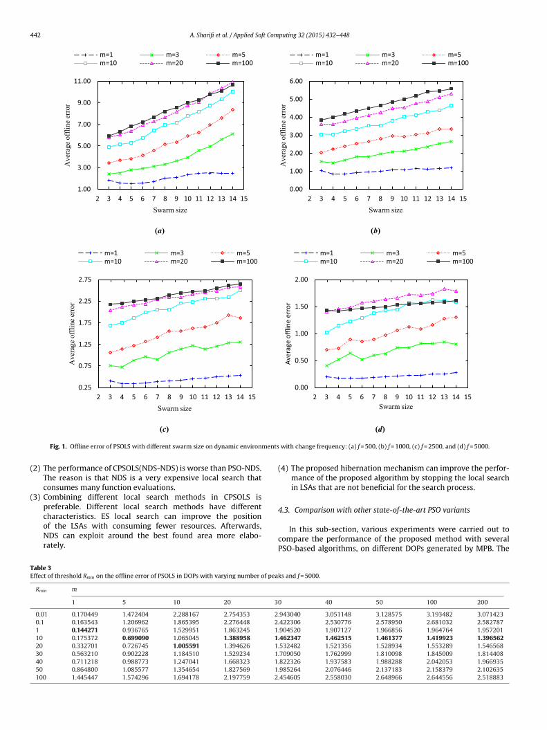
.2.1.1. Effect of the swarm size. In this set of experiments, wexamine the effect of the swarm size on the performance of PSOLSn different dynamic environments. Various experiments were car-ied out with value of the swarm size chosen from [3,14]. Thenvironmental parameters were the combination of change fre-uency f ∈ {500, 1000, 2500, 5000} and the number of peaks m ∈ {1,, 5, 10, 20, 100}.

Fig. 1 draws the average offline error of PSOLS with varyingwarm size across different dynamic environments. From Fig. 1,t can be seen that the swarm size 3 produces a better result in

ost of the tested DOPs. It can be also seen that the performance ofSOLS is degraded as the swarm size increases. The reason mainlyies in the fact that the swarm is responsible for creating LSAs inromising areas of the search space. The bigger the population sizef the swarm, the more function evaluations is consumed by thewarm for converging to an area. This makes less function evalua-ions available for LSAs to exploit the peaks.

Our experiments revealed that, the standard PSO with only threearticles fails to achieve a good performance due to the stagnation.owever, the proposed fuzzy social-only model can improve thexploration ability of PSO by its random behavior.

.2.1.2. Effect of the radius Rmin. The aim of this experiment is tonvestigate the effect of Rmin on the performance of PSOLS. As we

entioned in Section 3, Rmin is a threshold parameter which is

able 2efault parameter settings for PSOLS.

Parameter Value

Number of particles in the swarm 3c2 1.496180w 0.729844Rmin 10� 20.0ıinit 0.5b 0.2Smin 0.01� init 0.2

puting 32 (2015) 432–448 441

used to determine the convergence of the swarm. Therefore, it isexpected that this parameter has a significant impact on the per-formance of PSOLS.

From Table 3, it can be seen that PSOLS with Rmin = 10.0 givesbetter results. On the one hand, a large value of Rmin causes that theswarm creates LSAs in areas far away from the peaks. On the otherhand, a very small value of Rmin causes that the swarm consumesa large number of fitness evaluations to converge. In addition, asmall value of Rmin can cause the swarm to frequently converge toa limited area of the search space. Table 3 also indicates that theextreme values for this parameter, i.e. 0.01, 0.1 and 100, gives theworst results.

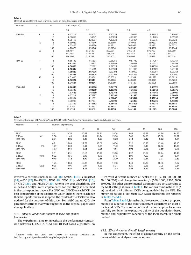
4.2.2. Effect of using different local search methodsThis set of experiments aims to investigate the effect of local

search method being used by each LSA on the performance of PSOLSin DOPs with different complexities. The environmental conditionswere different combinations of dimension d ∈ {5, 10, 100}, numberof peak m ∈ {1, 10, 100}, and severity s ∈ {0.0, 1.0, 2.0, 3.0, 4.0, 5.0}.The results are given in Table 4. From Table 4, it is observed thatNDS is the most favorable local search method in the majority ofthe tested DOPs.

4.2.3. Effect of collaboration between swarm and local searchagents

This experiment has been specifically designed to verify theeffectiveness of hybridizing PSO with local search agents. In thisexperiment, the performance of the proposed method is comparedwith two different methods: (1) re-randomization PSO, i.e. RPSOand (2) a group of independent local search agents (GILSAs). ForRPSO, a population size of 30 particles was used. Furthermore, thevelocity of particles was clamped within the range [−20, 20] andthe rate of re-randomization was set to 50%. For GILSAs, a numberof LSAs equal to the number of peaks in the landscape are randomlyinitialized into the search space. Each LSA then starts to explore thesearch space using NDS. To prevent LSAs from searching in the samearea, the exclusion operator with radius 20 is also applied.

The results of experiment conducted to investigate the effec-tiveness of hybridizing PSO with local search agents are listed inTable 5.

As shown in Table 5, all the results of the proposed hybridmethod are much better than the results of RPSO and GILSAs. Thecomparison results clearly confirm the advantages of collaborationbetween the swarm and LSAs in PSOLS.

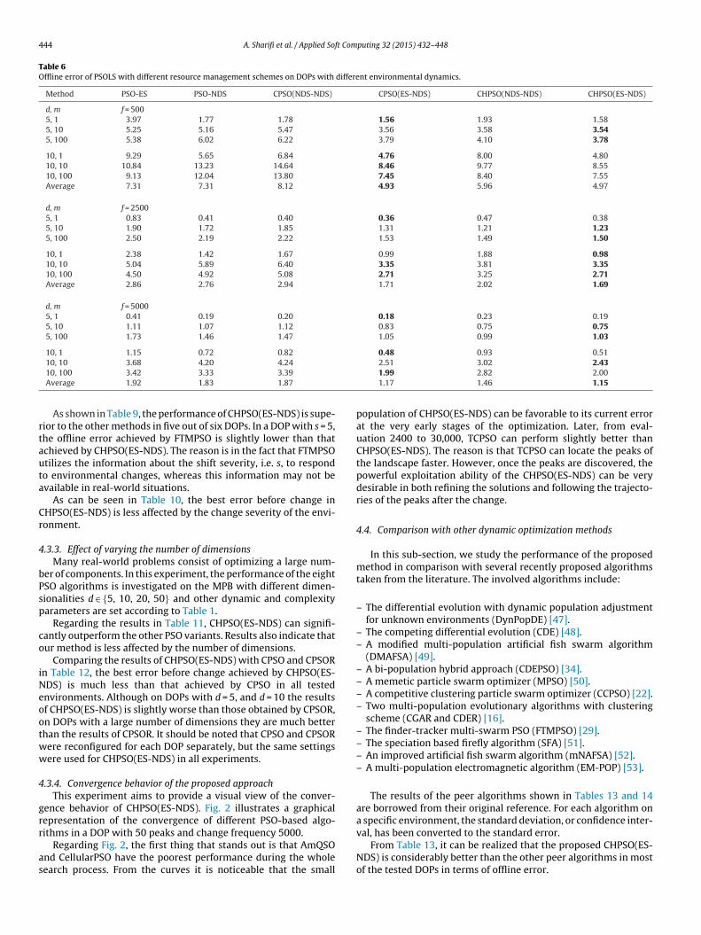
4.2.4. Effect of different resource management schemesThe most important component of the proposed adapted algo-

rithms is the resource management scheme that increases theefficiency of the PSOLS. Therefore, experiments were carried outto validate the benefits of the proposed adaptations. The main goalof this set of experiments is to specifically emphasize on the impor-tance of the managing function evaluations for DOPs. Furthermore,we are interested in investigating the effect of combining differentresource management schemes. The performance of different algo-rithms was evaluated on various DOPs with f ∈ {500, 2500, 5000},d ∈ {5, 10}, and m ∈ {1, 10, 100}. Experimental results are providedin Table 6. Table 6 indicates that managing function evaluations isa major concern that can contribute much to the performance ofPSOLS on dynamic environments.

Several conclusions can be drawn from Table 6. Here we high-light a number of important conclusions as follows:

(1) It is clearly observed that the resource management schemeshave a significant influence on the performance of the proposedapproach.

442 A. Sharifi et al. / Applied Soft Computing 32 (2015) 432–448

(a) (b)

1.00

3.00

5.00

7.00

9.00

11.00

2 3 4 5 6 7 8 9 10 11 12 13 14 15

Ave

rage

off

line

erro

r

Swarm size

m=1 m=3 m=5m=10 m=20 m=100

0.00

1.00

2.00

3.00

4.00

5.00

6.00

2 3 4 5 6 7 8 9 10 11 12 13 14 15

Ave

rage

off

line

erro

r

Swarm size

m=1 m=3 m=5m=10 m=20 m=100

0.25

0.75

1.25

1.75

2.25

2.75

2 3 4 5 6 7 8 9 10 11 12 13 14 15

Ave

rage

off

line

erro

r

Swarm size Swarm size

m=1 m=3 m=5m=10 m=20 m=100

0.00

0.50

1.00

1.50

2.00

2 3 4 5 6 7 8 9 10 11 12 13 14 15

Aver

age

offlin

e er

ror

m=1 m=3 m=5m=10 m=20 m=100

ments

(

(

TE

(c)

Fig. 1. Offline error of PSOLS with different swarm size on dynamic environ

2) The performance of CPSOLS(NDS-NDS) is worse than PSO-NDS.The reason is that NDS is a very expensive local search thatconsumes many function evaluations.

3) Combining different local search methods in CPSOLS ispreferable. Different local search methods have different
characteristics. ES local search can improve the positionof the LSAs with consuming fewer resources. Afterwards,NDS can exploit around the best found area more elabo-rately.
able 3ffect of threshold Rmin on the offline error of PSOLS in DOPs with varying number of pea

Rmin m

1 5 10 20 3

0.01 0.170449 1.472404 2.288167 2.754353 20.1 0.163543 1.206962 1.865395 2.276448 21 0.144271 0.936765 1.529951 1.863245 110 0.175372 0.699090 1.065045 1.388958 120 0.332701 0.726745 1.005591 1.394626 130 0.563210 0.902228 1.184510 1.529234 140 0.711218 0.988773 1.247041 1.668323 150 0.864800 1.085577 1.354654 1.827569 1100 1.445447 1.574296 1.694178 2.197759 2

(d)

with change frequency: (a) f = 500, (b) f = 1000, (c) f = 2500, and (d) f = 5000.

(4) The proposed hibernation mechanism can improve the perfor-mance of the proposed algorithm by stopping the local searchin LSAs that are not beneficial for the search process.

4.3. Comparison with other state-of-the-art PSO variants

In this sub-section, various experiments were carried out tocompare the performance of the proposed method with severalPSO-based algorithms, on different DOPs generated by MPB. The

ks and f = 5000.

0 40 50 100 200

.943040 3.051148 3.128575 3.193482 3.071423

.422306 2.530776 2.578950 2.681032 2.582787

.904520 1.907127 1.966856 1.964764 1.957201

.462347 1.462515 1.461377 1.419923 1.396562

.532482 1.521356 1.528934 1.553289 1.546568

.709050 1.762999 1.810098 1.845009 1.814408

.822326 1.937583 1.988288 2.042053 1.966935

.985264 2.076446 2.137183 2.158379 2.102635

.454605 2.558030 2.648966 2.644556 2.518883

A. Sharifi et al. / Applied Soft Computing 32 (2015) 432–448 443

Table 4Effect of using different local search methods on the offline error of PSOLS.

Method d m Shift length (s)

0.0 1.0 2.0 3.0 4.0 5.0

PSO-RW 5 1 0.45112 0.83071 1.40234 2.30422 3.58285 5.1268610 0.86069 1.58847 2.76093 4.22373 6.14465 8.35998

100 0.78117 2.24661 4.18529 6.35894 8.65815 11.052410 1 6.39022 8.76646 11.1169 15.4064 22.0227 28.5702

10 6.55826 9.86580 14.9211 20.9969 27.3431 34.5071100 4.76478 8.33540 13.0154 18.6546 24.6568 29.7344

50 1 850.497 836.136 862.561 846.742 870.700 875.35910 341.455 337.526 338.978 338.985 341.808 341.972

100 216.296 216.764 216.905 216.806 217.633 217.614

PSO-ES 5 1 0.18182 0.41204 0.65256 0.87743 1.17967 1.4326710 0.61517 1.10621 1.56895 1.96668 2.30917 2.69568

100 0.56870 1.72911 2.52528 3.14339 3.64598 4.0449210 1 0.50642 1.15019 1.84503 2.44935 3.07189 3.73131

10 1.99820 3.67536 5.02192 6.19992 7.26207 8.29264100 1.14821 3.42274 5.00106 6.34553 7.62520 8.77980

50 1 8.31006 16.2051 23.5525 31.0304 38.1722 47.581310 8.92927 14.9613 20.1166 24.0602 28.0973 31.5220

100 5.74614 10.9234 14.4799 17.6129 20.4908 23.0889

PSO-NDS 5 1 0.16546 0.20380 0.24179 0.29319 0.36372 0.4427010 0.85333 1.03259 1.16308 1.36187 1.52842 1.79575

100 1.11648 1.45459 1.79764 2.18646 2.57144 2.9808710 1 0.57711 0.72697 0.89392 1.01887 1.22884 1.50074

10 4.26594 4.11061 4.61842 5.03542 5.65114 6.39365100 3.38095 3.37294 3.70708 4.25223 4.90236 5.43897

50 1 7.27152 8.16682 8.88441 9.15409 9.75214 10.505510 15.3540 16.3572 16.9831 17.3668 17.2677 18.1880

100 12.4533 13.8362 14.1176 14.4144 15.1625 15.5804

Table 5Average offline error of RPSO, GILSAs, and PSOLS in DOPs with varying number of peaks and change intervals.

Method f Number of peaks (m)

1 5 10 20 30 40 50 100 200

RPSO500

9.41 19.74 20.48 20.21 19.24 18.48 17.79 15.96 14.27GILSAs 3.50 11.49 11.01 11.74 13.90 17.46 24.08 27.68 31.27PSO-NDS 2.31 4.86 5.87 6.23 6.28 6.14 6.12 6.02 5.74

RPSO1000

4.91 16.88 17.79 17.69 16.74 16.22 15.88 13.46 12.15GILSAs 1.77 10.20 9.43 7.75 7.40 7.99 8.43 16.02 19.29PSO-NDS 1.13 2.61 3.61 3.98 4.01 3.94 3.95 3.89 3.71

RPSO2500

2.91 14.51 16.15 15.77 15.08 14.22 13.94 12.24 10.46GILSAs 0.72 9.56 8.98 6.76 5.45 4.91 4.56 4.76 6.74PSO-NDS 0.45 1.12 1.90 2.18 2.29 2.25 2.24 2.21 2.13

15.36.81.5

i[Tmibtupa

4f

i

h

RPSO5000

1.75 13.64 15.22

GILSAs 0.35 9.06 9.07

PSO-NDS 0.22 0.57 1.13

nvolved algorithms include mQSO [18], AmQSO [45], CellularPSO24], mPSO [27], HmSO [28], APSO [46], CPSO [21] and CPSOR1 [16],P-CPSO [26], and FTMPSO [29]. Among the peer algorithms, theQSO and AmQSO were implemented for this study as described

n the corresponding papers. For CPSO and CPSOR on each DOP, theest configuration of the algorithms which enables them to achieveheir best performance is adopted. The results of TP-CPSO were alsopdated for the purposes of this paper. For mQSO and AmQSO, thearameter settings that were suggested in the original paper werelso applied here.

.3.1. Effect of varying the number of peaks and change
requencies
The experiment aims to investigate the performance compar-son between CHPSO(ES-NDS) and 10 PSO-based algorithms on

1 Source code for CPSO and CPSOR is publicly available at:ttp://cs.cug.edu.cn/teacherweb/lichanghe/pages/EAlib.html.

6 14.18 13.50 13.23 10.86 9.775 5.34 4.25 3.83 3.05 3.340 1.53 1.53 1.50 1.44 1.40

DOPs with different number of peaks m ∈ {1, 5, 10, 20, 30, 40,50, 100, 200} and change frequencies f ∈ {500, 1000, 2500, 5000,10,000}. The other environmental parameters are set according tothe MPB settings shown in Table 1. The various combinations of (f,m) resulted in 45 different DOPs being modeled by the MPB. Thenumerical results of different PSO-based algorithms are reportedin Tables 7 and 8.

From Tables 5 and 6, it can be clearly observed that our proposedmethod is superior to the other contestant algorithms on most ofthe tested DOPs. The results confirmed that our approach can suc-cessfully combine the explorative ability of the population-basedmethod and exploitative capability of the local search in a singlemethod.

4.3.2. Effect of varying the shift length severityIn this experiment, the effect of change severity on the perfor-

mance of different algorithms is examined.


Table 6Offline error of PSOLS with different resource management schemes on DOPs with different environmental dynamics.

Method PSO-ES PSO-NDS CPSO(NDS-NDS) CPSO(ES-NDS) CHPSO(NDS-NDS) CHPSO(ES-NDS)

d, m f = 5005, 1 3.97 1.77 1.78 1.56 1.93 1.585, 10 5.25 5.16 5.47 3.56 3.58 3.545, 100 5.38 6.02 6.22 3.79 4.10 3.78

10, 1 9.29 5.65 6.84 4.76 8.00 4.8010, 10 10.84 13.23 14.64 8.46 9.77 8.5510, 100 9.13 12.04 13.80 7.45 8.40 7.55Average 7.31 7.31 8.12 4.93 5.96 4.97

d, m f = 25005, 1 0.83 0.41 0.40 0.36 0.47 0.385, 10 1.90 1.72 1.85 1.31 1.21 1.235, 100 2.50 2.19 2.22 1.53 1.49 1.50

10, 1 2.38 1.42 1.67 0.99 1.88 0.9810, 10 5.04 5.89 6.40 3.35 3.81 3.3510, 100 4.50 4.92 5.08 2.71 3.25 2.71Average 2.86 2.76 2.94 1.71 2.02 1.69

d, m f = 50005, 1 0.41 0.19 0.20 0.18 0.23 0.195, 10 1.11 1.07 1.12 0.83 0.75 0.755, 100 1.73 1.46 1.47 1.05 0.99 1.03

10, 1 1.15 0.72 0.82 0.48 0.93 0.51

rtauta

Cr

4

bPsp

co

iNeootww

4

grr

as

10, 10 3.68 4.20 4.24

10, 100 3.42 3.33 3.39

Average 1.92 1.83 1.87

As shown in Table 9, the performance of CHPSO(ES-NDS) is supe-ior to the other methods in five out of six DOPs. In a DOP with s = 5,he offline error achieved by FTMPSO is slightly lower than thatchieved by CHPSO(ES-NDS). The reason is in the fact that FTMPSOtilizes the information about the shift severity, i.e. s, to respondo environmental changes, whereas this information may not bevailable in real-world situations.

As can be seen in Table 10, the best error before change inHPSO(ES-NDS) is less affected by the change severity of the envi-onment.

.3.3. Effect of varying the number of dimensionsMany real-world problems consist of optimizing a large num-

er of components. In this experiment, the performance of the eightSO algorithms is investigated on the MPB with different dimen-ionalities d ∈ {5, 10, 20, 50} and other dynamic and complexityarameters are set according to Table 1.

Regarding the results in Table 11, CHPSO(ES-NDS) can signifi-antly outperform the other PSO variants. Results also indicate thatur method is less affected by the number of dimensions.

Comparing the results of CHPSO(ES-NDS) with CPSO and CPSORn Table 12, the best error before change achieved by CHPSO(ES-DS) is much less than that achieved by CPSO in all testednvironments. Although on DOPs with d = 5, and d = 10 the resultsf CHPSO(ES-NDS) is slightly worse than those obtained by CPSOR,n DOPs with a large number of dimensions they are much betterhan the results of CPSOR. It should be noted that CPSO and CPSORere reconfigured for each DOP separately, but the same settingsere used for CHPSO(ES-NDS) in all experiments.

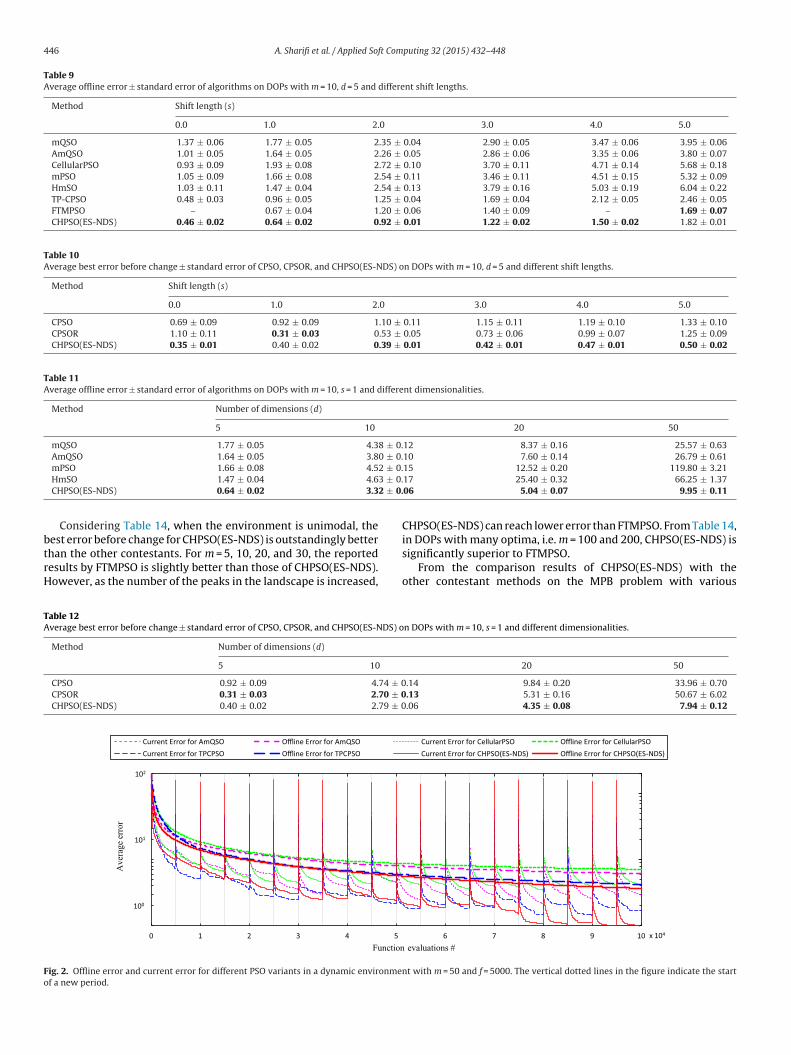
.3.4. Convergence behavior of the proposed approachThis experiment aims to provide a visual view of the conver-

ence behavior of CHPSO(ES-NDS). Fig. 2 illustrates a graphicalepresentation of the convergence of different PSO-based algo-
ithms in a DOP with 50 peaks and change frequency 5000.
Regarding Fig. 2, the first thing that stands out is that AmQSOnd CellularPSO have the poorest performance during the wholeearch process. From the curves it is noticeable that the small

2.51 3.02 2.431.99 2.82 2.001.17 1.46 1.15

population of CHPSO(ES-NDS) can be favorable to its current errorat the very early stages of the optimization. Later, from eval-uation 2400 to 30,000, TCPSO can perform slightly better thanCHPSO(ES-NDS). The reason is that TCPSO can locate the peaks ofthe landscape faster. However, once the peaks are discovered, thepowerful exploitation ability of the CHPSO(ES-NDS) can be verydesirable in both refining the solutions and following the trajecto-ries of the peaks after the change.

4.4. Comparison with other dynamic optimization methods

In this sub-section, we study the performance of the proposedmethod in comparison with several recently proposed algorithmstaken from the literature. The involved algorithms include:

– The differential evolution with dynamic population adjustmentfor unknown environments (DynPopDE) [47].

– The competing differential evolution (CDE) [48].– A modified multi-population artificial fish swarm algorithm

(DMAFSA) [49].– A bi-population hybrid approach (CDEPSO) [34].– A memetic particle swarm optimizer (MPSO) [50].– A competitive clustering particle swarm optimizer (CCPSO) [22].– Two multi-population evolutionary algorithms with clustering

scheme (CGAR and CDER) [16].– The finder-tracker multi-swarm PSO (FTMPSO) [29].– The speciation based firefly algorithm (SFA) [51].– An improved artificial fish swarm algorithm (mNAFSA) [52].– A multi-population electromagnetic algorithm (EM-POP) [53].

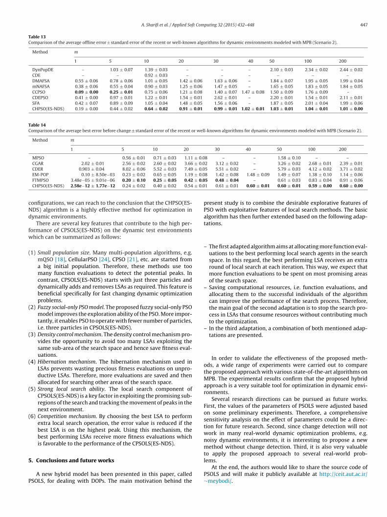
The results of the peer algorithms shown in Tables 13 and 14are borrowed from their original reference. For each algorithm ona specific environment, the standard deviation, or confidence inter-
val, has been converted to the standard error.
From Table 13, it can be realized that the proposed CHPSO(ES-NDS) is considerably better than the other peer algorithms in mostof the tested DOPs in terms of offline error.


Table 7Average offline error ± standard error of nine PSO-based algorithms on DOPs with d = 5, s = 1 and varying number of peaks and change intervals.

f m Method

mQSO AmQSO CellularPSO mPSO HmSO APSO TP-CPSO FTMPSO CHPSO(ES-NDS)

500 1 40.30 ± 1.30 10.41 ± 0.34 22.37 ± 3.87 8.71 ± 0.48 9.40 ± 0.31 4.81 ± 0.14 5.96 ± 0.22 1.76 ± 0.09 1.68 ± 0.035 11.50 ± 0.21 6.95 ± 0.12 14.20 ± 0.65 6.69 ± 0.26 7.83 ± 0.17 4.95 ± 0.11 5.12 ± 0.11 2.93 ± 0.18 2.97 ± 0.06

10 8.96 ± 0.19 6.97 ± 0.13 13.55 ± 0.52 7.19 ± 0.23 8.04 ± 0.14 5.16 ± 0.11 5.56 ± 0.11 3.91 ± 0.19 3.74 ± 0.0520 8.29 ± 0.11 7.61 ± 0.10 12.77 ± 0.38 8.01 ± 0.19 8.25 ± 0.12 5.81 ± 0.08 5.67 ± 0.10 4.83 ± 0.19 3.93 ± 0.0430 8.32 ± 0.09 8.99 ± 0.14 12.55 ± 0.42 8.43 ± 0.17 8.62 ± 0.12 6.03 ± 0.07 5.59 ± 0.08 5.05 ± 0.21 3.98 ± 0.0340 8.18 ± 0.08 10.26 ± 0.15 12.33 ± 0.38 8.62 ± 0.18 8.67 ± 0.12 6.10 ± 0.08 5.53 ± 0.07 – 3.92 ± 0.0350 8.12 ± 0.08 11.45 ± 0.17 12.19 ± 0.31 8.76 ± 0.18 8.81 ± 0.12 5.95 ± 0.06 5.57 ± 0.08 4.98 ± 0.15 3.86 ± 0.03

100 7.81 ± 0.08 12.35 ± 0.15 11.38 ± 0.29 8.91 ± 0.17 8.88 ± 0.11 6.08 ± 0.06 5.36 ± 0.06 5.31 ± 0.11 3.81 ± 0.02200 7.59 ± 0.07 12.82 ± 0.13 11.34 ± 0.27 8.88 ± 0.14 9.06 ± 0.11 6.20 ± 0.04 5.33 ± 0.05 5.52 ± 0.21 3.68 ± 0.02

1000 1 21.42 ± 0.69 6.15 ± 0.20 7.97 ± 0.54 4.44 ± 0.24 4.89 ± 0.16 2.72 ± 0.04 2.66 ± 0.08 0.89 ± 0.05 0.90 ± 0.025 6.32 ± 0.13 4.40 ± 0.11 6.16 ± 0.31 3.93 ± 0.16 4.46 ± 0.08 2.99 ± 0.09 2.67 ± 0.09 1.70 ± 0.10 1.71 ± 0.04

10 5.20 ± 0.10 4.50 ± 0.09 5.94 ± 0.23 4.57 ± 0.18 4.79 ± 0.07 3.87 ± 0.08 3.17 ± 0.06 2.36 ± 0.09 2.35 ± 0.0420 5.40 ± 0.08 4.74 ± 0.06 6.13 ± 0.17 4.97 ± 0.13 4.99 ± 0.08 4.13 ± 0.06 3.33 ± 0.06 3.01 ± 0.12 2.62 ± 0.0330 5.50 ± 0.06 4.79 ± 0.04 6.23 ± 0.15 5.15 ± 0.12 5.11 ± 0.07 4.12 ± 0.04 3.45 ± 0.06 3.06 ± 0.10 2.63 ± 0.0240 5.48 ± 0.07 4.80 ± 0.04 6.27 ± 0.15 5.17 ± 0.10 5.13 ± 0.06 4.15 ± 0.04 3.58 ± 0.05 – 2.54 ± 0.0250 5.31 ± 0.06 4.86 ± 0.04 6.26 ± 0.16 5.33 ± 0.10 5.15 ± 0.04 4.11 ± 0.03 3.57 ± 0.05 3.29 ± 0.10 2.52 ± 0.02

100 5.09 ± 0.05 4.91 ± 0.04 6.27 ± 0.14 5.60 ± 0.09 5.28 ± 0.05 4.26 ± 0.04 3.52 ± 0.04 3.63 ± 0.09 2.47 ± 0.01200 4.84 ± 0.05 5.18 ± 0.04 6.01 ± 0.11 5.78 ± 0.09 5.43 ± 0.05 4.21 ± 0.02 3.51 ± 0.04 3.74 ± 0.09 2.39 ± 0.01

2500 1 9.48 ± 0.31 2.44 ± 0.07 4.57 ± 0.31 1.79 ± 0.10 2.02 ± 0.07 1.06 ± 0.03 0.92 ± 0.03 0.39 ± 0.02 0.40 ± 0.015 3.33 ± 0.08 2.44 ± 0.08 3.15 ± 0.21 2.04 ± 0.12 2.12 ± 0.09 1.55 ± 0.05 1.17 ± 0.05 0.91 ± 0.08 0.78 ± 0.03

10 2.85 ± 0.07 2.65 ± 0.05 3.09 ± 0.16 2.66 ± 0.16 2.43 ± 0.07 2.17 ± 0.07 1.59 ± 0.06 1.21 ± 0.06 1.16 ± 0.0220 3.41 ± 0.06 2.99 ± 0.05 3.60 ± 0.13 3.07 ± 0.11 2.63 ± 0.05 2.51 ± 0.05 1.82 ± 0.04 1.66 ± 0.05 1.47 ± 0.0230 3.45 ± 0.05 3.01 ± 0.03 3.88 ± 0.12 3.15 ± 0.08 2.73 ± 0.04 2.61 ± 0.02 1.99 ± 0.04 1.87 ± 0.05 1.58 ± 0.0240 3.45 ± 0.04 3.04 ± 0.03 4.17 ± 0.12 3.17 ± 0.07 2.77 ± 0.04 2.59 ± 0.03 1.96 ± 0.03 – 1.56 ± 0.0150 3.38 ± 0.04 3.03 ± 0.03 4.25 ± 0.12 3.26 ± 0.07 2.76 ± 0.04 2.66 ± 0.02 2.01 ± 0.03 2.09 ± 0.07 1.58 ± 0.01

100 3.07 ± 0.03 2.96 ± 0.02 4.25 ± 0.13 3.31 ± 0.05 2.83 ± 0.03 2.62 ± 0.02 2.09 ± 0.03 2.22 ± 0.06 1.49 ± 0.01200 2.92 ± 0.02 2.93 ± 0.02 4.20 ± 0.09 3.36 ± 0.05 2.94 ± 0.02 2.64 ± 0.01 2.06 ± 0.02 2.22 ± 0.07 1.44 ± 0.01

5000 1 4.49 ± 0.14 1.27 ± 0.04 2.79 ± 0.19 0.90 ± 0.05 1.01 ± 0.03 0.53 ± 0.01 0.40 ± 0.01 0.18 ± 0.01 0.19 ± 0.005 1.72 ± 0.05 1.30 ± 0.06 1.94 ± 0.18 1.21 ± 0.12 1.23 ± 0.05 1.05 ± 0.06 0.75 ± 0.07 0.47 ± 0.05 0.44 ± 0.02

10 1.77 ± 0.05 1.64 ± 0.05 1.93 ± 0.08 1.66 ± 0.08 1.47 ± 0.04 1.31 ± 0.03 0.96 ± 0.05 0.67 ± 0.04 0.64 ± 0.0220 2.49 ± 0.05 2.03 ± 0.04 2.73 ± 0.12 2.05 ± 0.08 1.67 ± 0.04 1.69 ± 0.05 1.18 ± 0.03 0.93 ± 0.04 0.91 ± 0.0130 2.58 ± 0.04 2.11 ± 0.03 3.08 ± 0.11 2.18 ± 0.06 1.72 ± 0.03 1.78 ± 0.02 1.32 ± 0.03 1.14 ± 0.04 0.99 ± 0.0140 2.58 ± 0.04 2.18 ± 0.02 3.28 ± 0.11 2.24 ± 0.06 1.78 ± 0.03 1.86 ± 0.02 1.36 ± 0.03 – 1.02 ± 0.0150 2.50 ± 0.03 2.18 ± 0.02 3.34 ± 0.07 2.30 ± 0.04 1.75 ± 0.02 1.95 ± 0.02 1.40 ± 0.03 1.32 ± 0.04 1.03 ± 0.01

100 2.27 ± 0.02 2.14 ± 0.01 3.48 ± 0.11 2.32 ± 0.04 1.78 ± 0.02 1.95 ± 0.01 1.50 ± 0.02 1.61 ± 0.03 1.04 ± 0.01200 2.12 ± 0.02 2.12 ± 0.01 3.37 ± 0.08 2.34 ± 0.03 1.82 ± 0.01 1.90 ± 0.01 1.56 ± 0.02 1.67 ± 0.03 1.01 ± 0.00

10,000 1 2.34 ± 0.07 0.60 ± 0.01 1.63 ± 0.12 0.44 ± 0.02 0.52 ± 0.02 0.25 ± 0.01 0.20 ± 0.01 0.09 ± 0.00 0.09 ± 0.005 0.97 ± 0.04 0.75 ± 0.05 1.20 ± 0.15 0.72 ± 0.08 0.76 ± 0.07 0.57 ± 0.03 0.37 ± 0.03 0.31 ± 0.04 0.25 ± 0.01

10 1.10 ± 0.03 1.01 ± 0.04 1.19 ± 0.09 1.05 ± 0.10 0.90 ± 0.04 0.82 ± 0.02 0.54 ± 0.03 0.43 ± 0.03 0.40 ± 0.0120 1.89 ± 0.05 1.35 ± 0.03 2.13 ± 0.10 1.37 ± 0.06 1.09 ± 0.03 1.23 ± 0.02 0.74 ± 0.02 0.56 ± 0.01 0.52 ± 0.0130 1.98 ± 0.03 1.44 ± 0.02 2.59 ± 0.12 1.50 ± 0.06 1.14 ± 0.03 1.39 ± 0.02 0.82 ± 0.01 0.69 ± 0.09 0.58 ± 0.0140 2.01 ± 0.03 1.53 ± 0.02 2.72 ± 0.09 1.53 ± 0.05 1.19 ± 0.03 1.37 ± 0.01 0.93 ± 0.02 – 0.65 ± 0.0150 1.95 ± 0.03 1.55 ± 0.02 2.91 ± 0.11 1.62 ± 0.04 1.17 ± 0.01 1.46 ± 0.01 0.99 ± 0.01 0.86 ± 0.02 0.65 ± 0.01

100 1.75 ± 0.02 1.52 ± 0.01 3.02 ± 0.11 1.62 ± 0.03 1.15 ± 0.01 1.38 ± 0.01 1.19 ± 0.01 1.08 ± 0.03 0.65 ± 0.00200 1.60 ± 0.01 1.52 ± 0.01 2.94 ± 0.10 1.64 ± 0.02 1.15 ± 0.01 1.36 ± 0.01 1.29 ± 0.01 1.13 ± 0.04 0.67 ± 0.00

Table 8Average best error before change ± standard error of CPSO, CPSOR, and CHPSO(ES-NDS) on DOPs with d = 5, s = 1 and varying number of peaks and change intervals.

Method f Number of peaks (m)

1 5 10 20 30 40 50 100 200

CPSO500

67.88 ± 3.97 17.81 ± 0.49 15.65 ± 0.51 11.06 ± 0.42 8.92 ± 0.35 10.25 ± 0.36 9.26 ± 0.30 8.80 ± 0.29 7.09 ± 0.25CPSOR 14.03 ± 1.46 12.00 ± 0.94 11.38 ± 0.93 10.55 ± 0.79 7.87 ± 0.59 10.04 ± 0.68 9.26 ± 0.56 9.43 ± 0.52 7.95 ± 0.41CHPSO(ES-NDS) 0.02 ± 0.003 1.83 ± 0.06 2.60 ± 0.05 2.81 ± 0.04 2.78 ± 0.03 2.74 ± 0.03 2.69 ± 0.02 2.60 ± 0.02 2.52 ± 0.02

CPSO1000

12.26 ± 0.46 6.97 ± 0.17 7.12 ± 0.19 5.33 ± 0.14 4.75 ± 0.13 5.20 ± 0.15 5.02 ± 0.13 4.69 ± 0.14 3.78 ± 0.12CPSOR 1.41 ± 0.12 2.87 ± 0.14 2.98 ± 0.14 3.26 ± 0.12 2.88 ± 0.12 3.31 ± 0.14 3.72 ± 0.15 3.78 ± 0.14 3.49 ± 0.14CHPSO(ES-NDS) 5.90e−9 ± 3.02e−9 0.92 ± 0.04 1.60 ± 0.04 1.84 ± 0.03 1.83 ± 0.02 1.82 ± 0.02 1.81 ± 0.02 1.70 ± 0.01 1.63 ± 0.01

CPSO2500


CPSO5000


CPSO10,000

3.92e−5 ± 2.14e−4 0.69 ± 0.06 0.71 ± 0.09 1.11 ± 0.08 0.86 ± 0.06 0.87 ± 0.06 1.05 ± 0.06 1.01 ± 0.06 0.71 ± 0.04CPSOR 2.44e−3 ± 7.09e−3 0.36 ± 0.04 0.13 ± 0.02 0.54 ± 0.04 0.34 ± 0.03 0.49 ± 0.03 0.65 ± 0.05 0.84 ± 0.05 0.75 ± 0.04CHPSO(ES-NDS) 6.03e−13 ± 8.80e−14 0.15 ± 0.01 0.25 ± 0.01 0.33 ± 0.01 0.36 ± 0.01 0.38 ± 0.01 0.38 ± 0.01 0.34 ± 0.00 0.33 ± 0.00


Table 9Average offline error ± standard error of algorithms on DOPs with m = 10, d = 5 and different shift lengths.

Method Shift length (s)

0.0 1.0 2.0 3.0 4.0 5.0

mQSO 1.37 ± 0.06 1.77 ± 0.05 2.35 ± 0.04 2.90 ± 0.05 3.47 ± 0.06 3.95 ± 0.06AmQSO 1.01 ± 0.05 1.64 ± 0.05 2.26 ± 0.05 2.86 ± 0.06 3.35 ± 0.06 3.80 ± 0.07CellularPSO 0.93 ± 0.09 1.93 ± 0.08 2.72 ± 0.10 3.70 ± 0.11 4.71 ± 0.14 5.68 ± 0.18mPSO 1.05 ± 0.09 1.66 ± 0.08 2.54 ± 0.11 3.46 ± 0.11 4.51 ± 0.15 5.32 ± 0.09HmSO 1.03 ± 0.11 1.47 ± 0.04 2.54 ± 0.13 3.79 ± 0.16 5.03 ± 0.19 6.04 ± 0.22TP-CPSO 0.48 ± 0.03 0.96 ± 0.05 1.25 ± 0.04 1.69 ± 0.04 2.12 ± 0.05 2.46 ± 0.05FTMPSO – 0.67 ± 0.04 1.20 ± 0.06 1.40 ± 0.09 – 1.69 ± 0.07CHPSO(ES-NDS) 0.46 ± 0.02 0.64 ± 0.02 0.92 ± 0.01 1.22 ± 0.02 1.50 ± 0.02 1.82 ± 0.01

Table 10Average best error before change ± standard error of CPSO, CPSOR, and CHPSO(ES-NDS) on DOPs with m = 10, d = 5 and different shift lengths.

Method Shift length (s)

0.0 1.0 2.0 3.0 4.0 5.0

CPSO 0.69 ± 0.09 0.92 ± 0.09 1.10 ± 0.11 1.15 ± 0.11 1.19 ± 0.10 1.33 ± 0.10CPSOR 1.10 ± 0.11 0.31 ± 0.03 0.53 ± 0.05 0.73 ± 0.06 0.99 ± 0.07 1.25 ± 0.09CHPSO(ES-NDS) 0.35 ± 0.01 0.40 ± 0.02 0.39 ± 0.01 0.42 ± 0.01 0.47 ± 0.01 0.50 ± 0.02

Table 11Average offline error ± standard error of algorithms on DOPs with m = 10, s = 1 and different dimensionalities.

Method Number of dimensions (d)

5 10 20 50

mQSO 1.77 ± 0.05 4.38 ± 0.12 8.37 ± 0.16 25.57 ± 0.63AmQSO 1.64 ± 0.05 3.80 ± 0.10 7.60 ± 0.14 26.79 ± 0.61

2 ± 0.3 ± 0.2 ± 0.

btrH

TA

Fo

mPSO 1.66 ± 0.08 4.5HmSO 1.47 ± 0.04 4.6CHPSO(ES-NDS) 0.64 ± 0.02 3.3

Considering Table 14, when the environment is unimodal, the
est error before change for CHPSO(ES-NDS) is outstandingly betterhan the other contestants. For m = 5, 10, 20, and 30, the reportedesults by FTMPSO is slightly better than those of CHPSO(ES-NDS).owever, as the number of the peaks in the landscape is increased,
able 12verage best error before change ± standard error of CPSO, CPSOR, and CHPSO(ES-NDS) o

Method Number of dimensions (d)

5 10

CPSO 0.92 ± 0.09 4.74 ± 0CPSOR 0.31 ± 0.03 2.70 ± 0CHPSO(ES-NDS) 0.40 ± 0.02 2.79 ± 0

100

101

102

0 1 2 3 4 5

Ave

rage

err

or

Current E rror for AmQSO Offli ne Error for AmQSOCurrent E rror for TP CPSO Offli ne Error for TP CPSO

Funct ion

ig. 2. Offline error and current error for different PSO variants in a dynamic environmef a new period.

15 12.52 ± 0.20 119.80 ± 3.2117 25.40 ± 0.32 66.25 ± 1.3706 5.04 ± 0.07 9.95 ± 0.11

CHPSO(ES-NDS) can reach lower error than FTMPSO. From Table 14,
in DOPs with many optima, i.e. m = 100 and 200, CHPSO(ES-NDS) issignificantly superior to FTMPSO.
From the comparison results of CHPSO(ES-NDS) with theother contestant methods on the MPB problem with various

n DOPs with m = 10, s = 1 and different dimensionalities.

20 50

.14 9.84 ± 0.20 33.96 ± 0.70

.13 5.31 ± 0.16 50.67 ± 6.02

.06 4.35 ± 0.08 7.94 ± 0.12

6 7 8 9 10 x 104

Current E rror for Cell ularPSO Offli ne Error for Cell ularPSOCurrent E rror for CH PSO(ES-ND S) Offli ne Error for CH PSO(ES-ND S)

evaluations #

nt with m = 50 and f = 5000. The vertical dotted lines in the figure indicate the start


Table 13Comparison of the average offline error ± standard error of the recent or well-known algorithms for dynamic environments modeled with MPB (Scenario 2).

Method m

1 5 10 20 30 40 50 100 200

DynPopDE – 1.03 ± 0.07 1.39 ± 0.03 – – – 2.10 ± 0.03 2.34 ± 0.02 2.44 ± 0.02CDE – – 0.92 ± 0.03 – – – – – –DMAFSA 0.55 ± 0.06 0.78 ± 0.06 1.01 ± 0.05 1.42 ± 0.06 1.63 ± 0.06 – 1.84 ± 0.07 1.95 ± 0.05 1.99 ± 0.04mNAFSA 0.38 ± 0.06 0.55 ± 0.04 0.90 ± 0.03 1.25 ± 0.06 1.47 ± 0.05 – 1.65 ± 0.05 1.83 ± 0.05 1.84 ± 0.05CCPSO 0.09 ± 0.00 0.25 ± 0.01 0.75 ± 0.06 1.21 ± 0.08 1.40 ± 0.07 1.47 ± 0.08 1.50 ± 0.09 1.76 ± 0.09 -CDEPSO 0.41 ± 0.00 0.97 ± 0.01 1.22 ± 0.01 1.54 ± 0.01 2.62 ± 0.01 – 2.20 ± 0.01 1.54 ± 0.01 2.11 ± 0.01SFA 0.42 ± 0.07 0.89 ± 0.09 1.05 ± 0.04 1.48 ± 0.05 1.56 ± 0.06 – 1.87 ± 0.05 2.01 ± 0.04 1.99 ± 0.06CHPSO(ES-NDS) 0.19 ± 0.00 0.44 ± 0.02 0.64 ± 0.02 0.91 ± 0.01 0.99 ± 0.01 1.02 ± 0.01 1.03 ± 0.01 1.04 ± 0.01 1.01 ± 0.00

Table 14Comparison of the average best error before change ± standard error of the recent or well-known algorithms for dynamic environments modeled with MPB (Scenario 2).

Method m

1 5 10 20 30 40 50 100 200

MPSO – 0.56 ± 0.01 0.71 ± 0.03 1.11 ± 0.08 – – 1.58 ± 0.10 – –CGAR 2.02 ± 0.01 2.56 ± 0.02 2.60 ± 0.02 3.66 ± 0.02 3.12 ± 0.02 – 3.26 ± 0.02 2.68 ± 0.01 2.39 ± 0.01CDER 0.903 ± 0.04 8.02 ± 0.06 5.52 ± 0.03 7.49 ± 0.05 5.51 ± 0.02 – 5.79 ± 0.03 4.12 ± 0.02 3.71 ± 0.02

± 0.0 ± 0.0 ± 0.0

cNd

fw

(

(

(

(

(

(

5

P

noisy dynamic environments, it is interesting to propose a newmethod without change detection. Third, it is also very valuableto apply the proposed approach to several real-world prob-

EM-POP 0.10 ± 8.50e−03 0.23 ± 0.02 0.65 ± 0.05 1.19FTMPSO 3.48e−05 ± 9.01e−06 0.20 ± 0.10 0.25 ± 0.05 0.42CHPSO(ES-NDS) 2.58e−12 ± 1.77e−12 0.24 ± 0.02 0.40 ± 0.02 0.54

onfigurations, we can reach to the conclusion that the CHPSO(ES-DS) algorithm is a highly effective method for optimization inynamic environments.

There are several key features that contribute to the high per-ormance of CPSOLS(ES-NDS) on the dynamic test environmentshich can be summarized as follows:

1) Small population size. Many multi-population algorithms, e.g.mQSO [18], CellularPSO [24], CPSO [21], etc. are started froma big initial population. Therefore, these methods use toomany function evaluations to detect the potential peaks. Incontrast, CPSOLS(ES-NDS) starts with just three particles anddynamically adds and removes LSAs as required. This feature isbeneficial specifically for fast changing dynamic optimizationproblems.

2) Fuzzy social-only PSO model. The proposed fuzzy social-only PSOmodel improves the exploration ability of the PSO. More impor-tantly, it enables PSO to operate with fewer number of particles,i.e. three particles in CPSOLS(ES-NDS).

3) Density control mechanism. The density control mechanism pro-vides the opportunity to avoid too many LSAs exploiting thesame sub-area of the search space and hence save fitness eval-uations.

4) Hibernation mechanism. The hibernation mechanism used inLSAs prevents wasting precious fitness evaluations on unpro-ductive LSAs. Therefore, more evaluations are saved and thenallocated for searching other areas of the search space.

5) Strong local search ability. The local search component ofCPSOLS(ES-NDS) is a key factor in exploiting the promising sub-regions of the search and tracking the movement of peaks in thenext environment.

6) Competition mechanism. By choosing the best LSA to performextra local search operation, the error value is reduced if thebest LSA is on the highest peak. Using this mechanism, thebest performing LSAs receive more fitness evaluations whichis favorable to the performance of the CPSOLS(ES-NDS).

. Conclusions and future works

A new hybrid model has been presented in this paper, calledSOLS, for dealing with DOPs. The main motivation behind the

8 1.42 ± 0.08 1.48 ± 0.09 1.49 ± 0.07 1.38 ± 0.10 1.14 ± 0.065 0.48 ± 0.04 – 0.61 ± 0.03 0.83 ± 0.04 0.91 ± 0.061 0.61 ± 0.01 0.60 ± 0.01 0.60 ± 0.01 0.59 ± 0.00 0.60 ± 0.00

present study is to combine the desirable explorative features ofPSO with exploitative features of local search methods. The basicalgorithm has then further extended based on the following adap-tations.

– The first adapted algorithm aims at allocating more function eval-uations to the best performing local search agents in the searchspace. In this regard, the best performing LSA receives an extraround of local search at each iteration. This way, we expect thatmore function evaluations to be spent on most promising areasof the search space.

– Saving computational resources, i.e. function evaluations, andallocating them to the successful individuals of the algorithmcan improve the performance of the search process. Therefore,the main goal of the second adaptation is to stop the search pro-cess in LSAs that consume resources without contributing muchto the optimization.

– In the third adaptation, a combination of both mentioned adap-tations are presented.

In order to validate the effectiveness of the proposed meth-ods, a wide range of experiments were carried out to comparethe proposed approach with various state-of-the-art algorithms onMPB. The experimental results confirm that the proposed hybridapproach is a very suitable tool for optimization in dynamic envi-ronments.

Several research directions can be pursued as future works.First, the values of the parameters of PSOLS were adjusted basedon some preliminary experiments. Therefore, a comprehensivesensitivity analysis on the effect of parameters could be a direc-tion for future research. Second, since change detection will notwork in many real-world dynamic optimization problems, e.g.

lems.At the end, the authors would like to share the source code of

PSOLS and will make it publicly available at http://ceit.aut.ac.ir/∼meybodi/.

http://ceit.aut.ac.ir/~meybodi/







4 ft Com

R

[

[

[

[

[

[

[

[

[

[

[

[

[

[

[

[

[

[

[

[

[

[

[

[

[

[

[

[

[

[

[

[

[

[

[

[

[

[

[

[

[

[


eferences

[1] C. Li, S. Yang, D.A. Pelta, Benchmark Generator for the IEEE WCCI-2012 Com-petition on Evolutionary Computation for Dynamic Optimization Problems,2011.

[2] T. Blackwell, Particle swarm optimization in dynamic environments, in: S. Yang,Y.-S. Ong, Y. Jin (Eds.), Evolutionary Computation in Dynamic and UncertainEnvironments, Springer, Berlin, Heidelberg, 2007, pp. 29–49.

[3] J. Kennedy, R. Eberhart, Particle swarm optimization, in: International Confer-ence on Neural IEEE. Networks, 1995, pp. 1942–1948.

[4] S. Sun, J. Li, A two-swarm cooperative particle swarms optimization, SwarmEvol. Comput. 15 (2014) 1–18.

[5] B.-Y. Qu, P.N. Suganthan, S. Das, A distance-based locally informed particleswarm model for multimodal optimization, IEEE Trans. Evol. Comput. 17 (2013)387–402.

[6] G. Fornarelli, A. Giaquinto, An unsupervised multi-swarm clustering techniquefor image segmentation, Swarm Evol. Comput. 11 (2013) 31–45.

[7] A.S. Rakitianskaia, A.P. Engelbrecht, Training feedforward neural networkswith dynamic particle swarm optimisation, Swarm Intell. 6 (2012)233–270.

[8] Y. Yan, L. Osadciw, Density estimation using a new dimension adaptive particleswarm optimization algorithm, Swarm Intell. 3 (2009) 275–301.

[9] N.C. Sahoo, S. Ganguly, D. Das, Multi-objective planning of electrical distribu-tion systems incorporating sectionalizing switches and tie-lines using particleswarm optimization, Swarm Evol. Comput. 3 (2012) 15–32.

10] A.A. Mousa, M.A. El-Shorbagy, W.F. Abd-El-Wahed, Local search based hybridparticle swarm optimization algorithm for multiobjective optimization, SwarmEvol. Comput. 3 (2012) 1–14.

11] S. Alam, G. Dobbie, Y.S. Koh, P. Riddle, S. Ur Rehman, Research on particleswarm optimization based clustering: a systematic review of literature andtechniques, Swarm Evol. Comput. 17 (2014) 1–13.

12] R.C. Xiaohui Hu, Eberhart, Adaptive particle swarm optimization: detectionand response to dynamic systems, in: Proceedings of the 2002 Congress onEvolutionary Computation, 2002, pp. 1666–1670.

13] T.M. Blackwell, P. Bentley, Don’t push me! Collision-avoiding swarms, in:Proceedings of the 2002 Congress on Evolutionary Computation, 2002, pp.1691–1696.

14] T.M. Blackwell, Dynamic search with charged, in: Genetic and EvolutionaryComputation Conference, 2002, pp. 9–13.

15] S. Janson, M. Middendorf, A hierarchical particle swarm optimizer for noisy anddynamic environments, Genet. Program Evol. Mach. 7 (2006) 329–354.

16] C. Li, S. Yang, A general framework of multipopulation methods with clusteringin undetectable dynamic environments, IEEE Trans. Evol. Comput. 16 (2012)556–577.

17] H. Wang, D. Wang, S. Yang, Triggered memory-based swarm optimization indynamic environments, in: V Giacobini (Ed.), Applications of Evolutionary Com-puting, Springer, Berlin, Heidelberg, 2007, pp. 637–646.

18] T. Blackwell, J. Branke, Multiswarms, exclusion, and anti-convergence indynamic environments, IEEE Trans. Evol. Comput. 10 (2006) 459–472.

19] U. Halder, S. Das, D. Maity, A cluster-based differential evolution algorithmwith external archive for optimization in dynamic environments, IEEE Trans.Cybern. 43 (2013) 881–897.

20] D. Parrott, Li Xiaodong, Locating and tracking multiple dynamic optima by aparticle swarm model using speciation, IEEE Trans. Evol. Comput. 10 (2006)440–458.

21] S. Yang, C. Li, A clustering particle swarm optimizer for locating and trackingmultiple optima in dynamic environments, IEEE Trans. Evol. Comput. 14 (2010)959–974.

22] A. Nickabadi, M. Ebadzadeh, R. Safabakhsh, A competitive clustering particleswarm optimizer for dynamic optimization problems, Swarm Intell. 6 (2012)177–206.

23] A. Nickabadi, M.M. Ebadzadeh, R. Safabakhsh, A novel particle swarm opti-mization algorithm with adaptive inertia weight, Appl. Soft Comput. 11 (2011)3658–3670.

24] A. Hashemi, M.R. Meybodi, Cellular PSO: a PSO for dynamic environments, in:Z. Cai, Z. Li, Z. Kang, Y. Liu (Eds.), Advances in Computation and Intelligence,Springer, Berlin, Heidelberg, 2009, pp. 422–433.

25] A.B. Hashemi, M.R. Meybodi, A multi-role cellular PSO for dynamic envi-ronments, in: 14th International CSI Computer Conference, 2009, pp.
412–417.
26] A. Sharifi, V. Noroozi, M. Bashiri, A.B. Hashemi, M.R. Meybodi, Two phased cel-lular PSO: a new collaborative cellular algorithm for optimization in dynamicenvironments, in: IEEE Congress on Evolutionary Computation, 2012, pp.1–8.

[

[

puting 32 (2015) 432–448

27] M. Kamosi, A. Hashemi, M.R. Meybodi, New particle swarm optimization algo-rithm for dynamic environments, in: B. Panigrahi, S. Das, P. Suganthan, S. Dash(Eds.), Swarm, Evolutionary, and Memetic Computing, Springer, Berlin, Heidel-berg, 2010, pp. 129–138.

28] M. Kamosi, A.B. Hashemi, M.R. Meybodi, A hibernating multi-swarm optimiza-tion algorithm for dynamic environments, in: Nature and Biologically InspiredComputing (NaBIC), 2010 Second World Congress On, 2010, pp. 363–369.

29] D. Yazdani, B. Nasiri, A. Sepas-Moghaddam, M.R. Meybodi, A novel multi-swarmalgorithm for optimization in dynamic environments based on particle swarmoptimization, Appl. Soft Comput. 13 (2013) 2144–2158.

30] L. Liu, S. Yang, D. Wang, Particle swarm optimization with composite particlesin dynamic environments, IEEE Trans. Syst. Man Cybern. B: Cybern. 40 (2010)1634–1648.

31] J. Karimi, H. Nobahari, S.H. Pourtakdoust, A new hybrid approach for dynamiccontinuous optimization problems, Appl. Soft Comput. 12 (2012) 1158–1167.

32] R.I. Lung, D. Dumitrescu, A collaborative model for tracking optima in dynamicenvironments, in: IEEE Congress on Evolutionary Computation, 2007, pp.564–567.

33] R. Lung, D. Dumitrescu, Evolutionary swarm cooperative optimization indynamic environments, Nat Comput. 9 (2010) 83–94.

34] J.K. Kordestani, A. Rezvanian, M. Meybodi, CDEPSO: a bi-population hybridapproach for dynamic optimization problems, Appl. Intell. 40 (4) (2014)682–694.

35] H. Wang, S. Yang, W.H. Ip, D. Wang, A particle swarm optimization basedmemetic algorithm for dynamic optimization problems, Nat Comput. 9 (2010)703–725.

36] H.-G. Beyer, H.-P. Schwefel, Evolution strategies – a comprehensive introduc-tion, Nat. Comput. 1 (2002) 3–52.

37] P. Novoa-Hernández, C. Corona, D. Pelta, Efficient multi-swarm PSO algorithmsfor dynamic environments, Memet. Comput. 3 (2011) 163–174.

38] J. Branke, Memory enhanced evolutionary algorithms for changing opti-mization problems, in: Proceedings of the 1999 Congress on EvolutionaryComputation, Vol. 3, Washington, DC, 1999, p. 1882.

39] J. Branke, Evolutionary Optimization in Dynamic Environments, Kluwer Aca-demic Publishers, 2002.

40] J. Branke, H. Schmeck, Designing evolutionary algorithms for dynamic opti-mization problems, in: A. Ghosh, S. Tsutsui (Eds.), Advances in EvolutionaryComputing, Springer, Berlin, Heidelberg, 2003, pp. 239–262.

41] K. Trojanowski, Z. Michalewicz, Searching for optima in non-stationary envi-ronments, in: Proceedings of the 1999 Congress on Evolutionary Computation,1999, pp. 1843–1850.

42] T.T. Nguyen, S. Yang, J. Branke, Evolutionary dynamic optimization: a survey ofthe state of the art, Swarm Evol. Comput. 6 (2012) 1–24.

43] A.E. Ranginkaman, J. Kazemi Kordestani, A. Rezvanian, M.R. Meybodi, A note onthe paper “A multi-population harmony search algorithm with external archivefor dynamic optimization problems” by Turky and Abdullah, Inf. Sci. 288 (2014)12–14.

44] S. Holm, A simple sequentially rejective multiple test procedure, Scand. J. Stat.(1979) 65–70.

45] T. Blackwell, J. Branke, X. Li, Particle swarms for dynamic optimization prob-lems, in: C. Blum, D. Merkle (Eds.), Swarm Intelligence, Springer, Berlin,Heidelberg, 2008, pp. 193–217.

46] I. Rezazadeh, M. Meybodi, A. Naebi, Adaptive particle swarm optimizationalgorithm for dynamic environments, in: Y. Tan, Y. Shi, Y. Chai, G. Wang(Eds.), Advances in Swarm Intelligence, Springer, Berlin, Heidelberg, 2011, pp.120–129.

47] M. Plessis, A. Engelbrecht, Differential evolution for dynamic environmentswith unknown numbers of optima, J. Glob. Optim. 55 (2013) 73–99.

48] M.C. du Plessis, A.P. Engelbrecht, Using competitive population evaluation ina differential evolution algorithm for dynamic environments, Eur. J. Oper. Res.218 (2012) 7–20.

49] D. Yazdani, M.R. Akbarzadeh-Totonchi, B. Nasiri, M.R. Meybodi, A new artificialfish swarm algorithm for dynamic optimization problems, in: IEEE Congress onEvolutionary Computation, 2012, pp. 1–8.

50] H. Wang, S. Yang, W.H. Ip, D. Wang, A memetic particle swarm optimisationalgorithm for dynamic multi-modal optimisation problems, Int. J. Syst. Sci. 43(2012) 1268–1283.

51] B. Nasiri, M.R. Meybodi, Speciation based firefly algorithm for optimization indynamic environments, Int. J. Artif. Intell. 8 (2012) 118–132.

52] D. Yazdani, B. Nasiri, A. Sepas-Moghaddam, M. Meybodi, M. Akbarzadeh-Totonchi, mNAFSA: a novel approach for optimization in dynamic environ-ments with global changes, Swarm Evol. Comput. 18 (2014) 38–53.

53] A.M. Turky, S. Abdullah, A multi-population electromagnetic algorithm fordynamic optimisation problems, Appl. Soft Comput. 22 (2014) 474–482.

http://refhub.elsevier.com/S1568-4946(15)00214-8/sbref0270







































































































































































































































































































































































































































































































































































































































































































































































































































































































































































































































































































































































































































































































































































































Documents

Applied Soft Computing - Amirkabir University of Technologyce.aut.ac.ir/~meybodi/paper/Sharifi-ff-Kazemi-Mahdavian-meybodi... · A. Shariﬁ et al. / Applied Soft Computing 32 (2015)