Applied Statistics and Probability for Engineershaalshraideh/Courses/IE347/ch09.pdf · Applied Statistics and Probability for Engineers ... 9-9.3 Comparison to the t-test ... hypothesized

Copyright © 2014 John Wiley & Sons, Inc. All rights reserved.

Chapter 9

Tests of Hypotheses for a Single Sample

Applied Statistics and Probability for

Engineers

Sixth Edition

Douglas C. Montgomery George C. Runger


Chapter 9 Title and Outline

9 Tests of Hypotheses

for a Single Sample

9-1 Hypothesis Testing

9-1.1 Statistical Hypotheses

9-1.2 Tests of Statistical Hypotheses

9-1.3 1-Sided & 2-Sided Hypotheses

9-1.4 P-Values in Hypothesis Tests

9-1.5 Connection between Hypothesis

Tests & Confidence Intervals

9-1.6 General Procedure for

Hypothesis Tests

9-2 Tests on the Mean of a Normal

Distribution, Variance Known9-2.1 Hypothesis Tests on the Mean

9-2.2 Type II Error & Choice of Sample Size

9-2.3 Large-Sample Test

9-3 Tests on the Mean of a Normal

Distribution, Variance Unknown

9-3.1 Hypothesis Tests on the Mean


9-4 Tests of the Variance & Standard

Deviation of a Normal Distribution.9-4.1 Hypothesis Tests on the Variance


9-5 Tests on a Population Proportion

9-5.1 Large-Sample Tests on a Proportion


9-6 Summary Table of Inference Procedures

for a Single Sample

9-7 Testing for Goodness of Fit

9-8 Contingency Table Tests

9-9 Non-Parametric Procedures

9-9.1 The Sign Test

9-9.2 The Wilcoxon Signed-Rank Test

9-9.3 Comparison to the t-test

CHAPTER OUTLINE

2


9-1 Hypothesis Testing

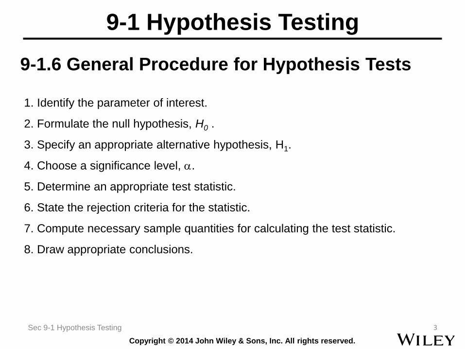
9-1.6 General Procedure for Hypothesis Tests

1. Identify the parameter of interest.

2. Formulate the null hypothesis, H0 .

3. Specify an appropriate alternative hypothesis, H1.

4. Choose a significance level, .

5. Determine an appropriate test statistic.

6. State the rejection criteria for the statistic.

7. Compute necessary sample quantities for calculating the test statistic.

8. Draw appropriate conclusions.

3Sec 9-1 Hypothesis Testing



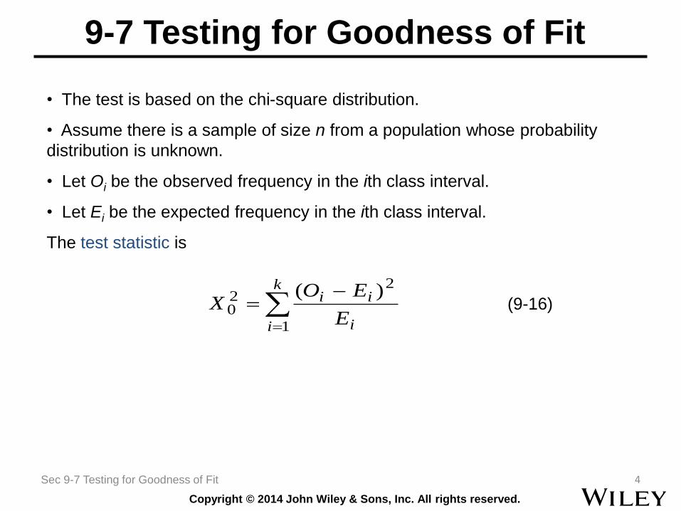
• The test is based on the chi-square distribution.

• Assume there is a sample of size n from a population whose probability

distribution is unknown.

• Let Oi be the observed frequency in the ith class interval.

• Let Ei be the expected frequency in the ith class interval.

The test statistic is

(9-16)

4Sec 9-7 Testing for Goodness of Fit

k

i i

ii

E

EOX

1

220

)(




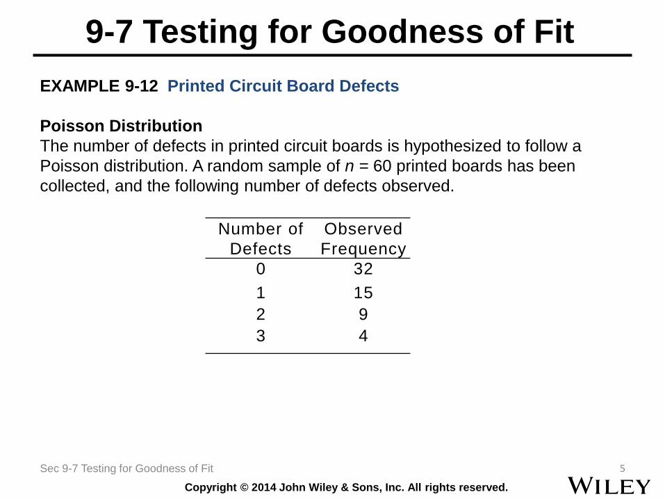
EXAMPLE 9-12 Printed Circuit Board Defects

Poisson Distribution

The number of defects in printed circuit boards is hypothesized to follow a

Poisson distribution. A random sample of n = 60 printed boards has been

collected, and the following number of defects observed.

Number of

Defects

Observed

Frequency

0 32

1 15

2 9

3 4


9-7 Testing for Goodness of Fit Example 9-12


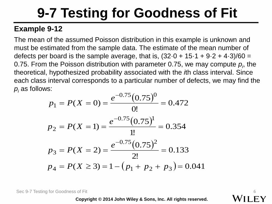
The mean of the assumed Poisson distribution in this example is unknown and

must be estimated from the sample data. The estimate of the mean number of

defects per board is the sample average, that is, (32·0 + 15·1 + 9·2 + 4·3)/60 =

0.75. From the Poisson distribution with parameter 0.75, we may compute pi, the

theoretical, hypothesized probability associated with the ith class interval. Since

each class interval corresponds to a particular number of defects, we may find the

pi as follows:

041.01)3(

133.0!2

75.0)2(

354.0!1

75.0)1(

472.0!0

75.0)0(

3214

275.0

3

175.0

2

075.0

1

pppXPp

eXPp

eXPp

eXPp




Example 9-12

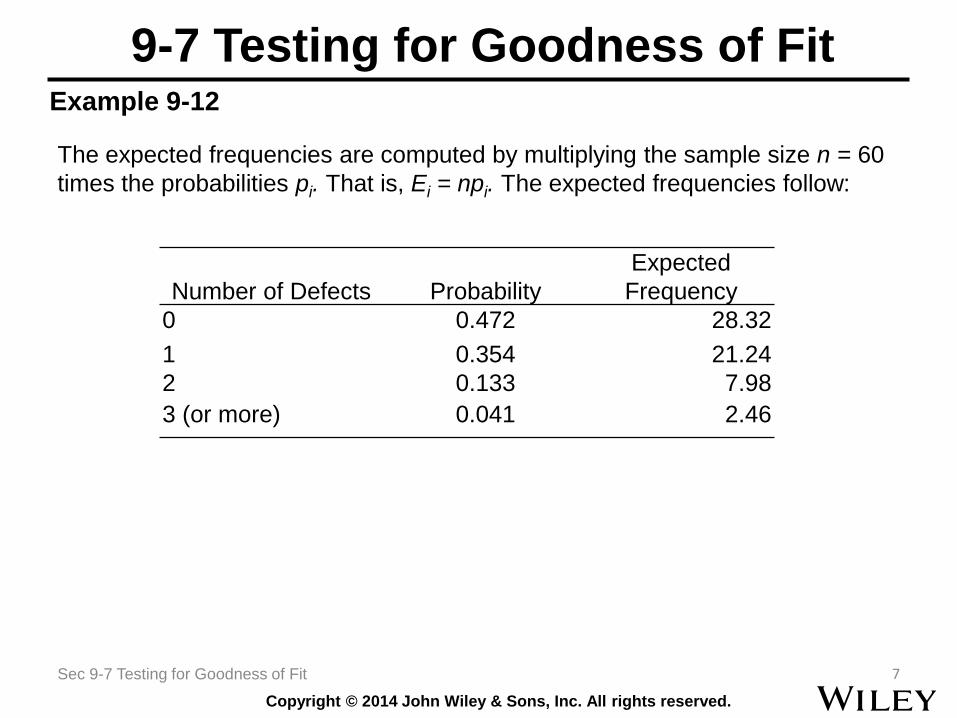
The expected frequencies are computed by multiplying the sample size n = 60

times the probabilities pi. That is, Ei = npi. The expected frequencies follow:

Number of Defects Probability

Expected

Frequency

0 0.472 28.32

1 0.354 21.24

2 0.133 7.98

3 (or more) 0.041 2.46




Example 9-12

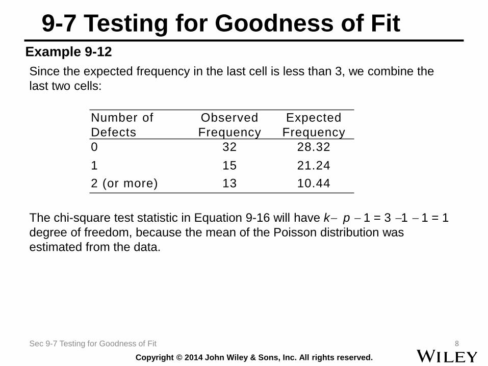
Since the expected frequency in the last cell is less than 3, we combine the

last two cells:

The chi-square test statistic in Equation 9-16 will have k p 1 = 3 1 1 = 1

degree of freedom, because the mean of the Poisson distribution was

estimated from the data.

Number of

Defects

Observed

Frequency

Expected

Frequency

0 32 28.32

1 15 21.24

2 (or more) 13 10.44




Example 9-12

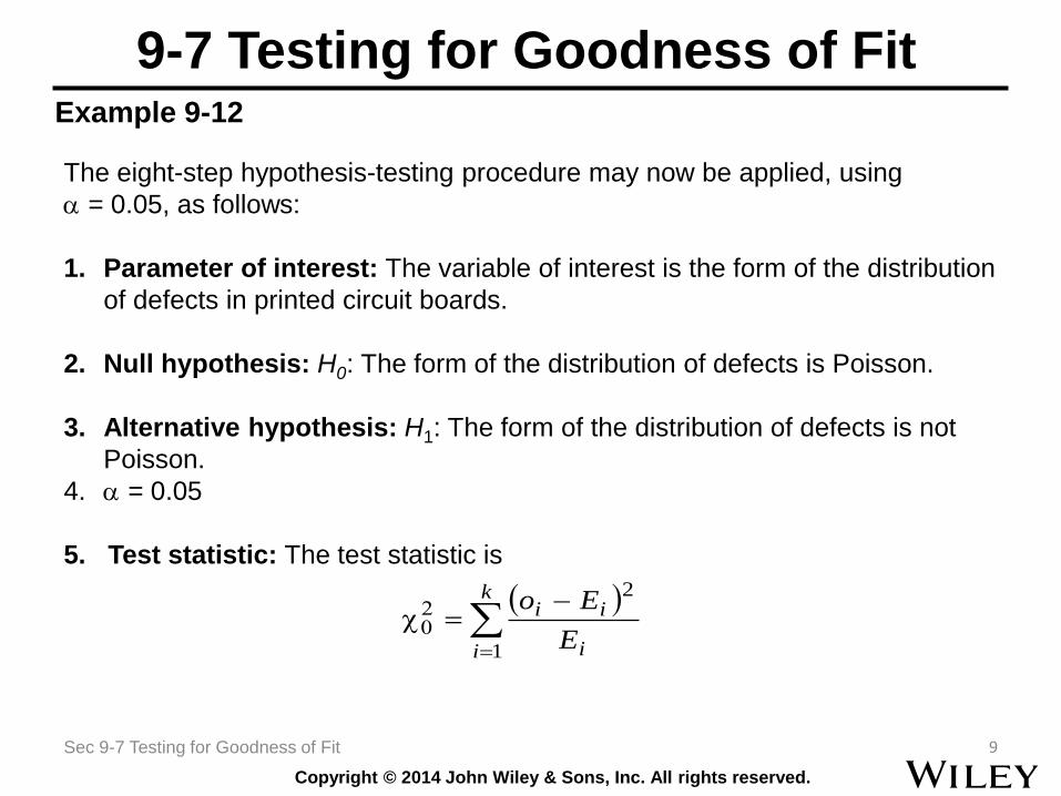
The eight-step hypothesis-testing procedure may now be applied, using

= 0.05, as follows:

1. Parameter of interest: The variable of interest is the form of the distribution

of defects in printed circuit boards.

2. Null hypothesis: H0: The form of the distribution of defects is Poisson.

3. Alternative hypothesis: H1: The form of the distribution of defects is not

Poisson.

4. = 0.05

5. Test statistic: The test statistic is

k

i i

ii

E

Eo

1

2




Example 9-12

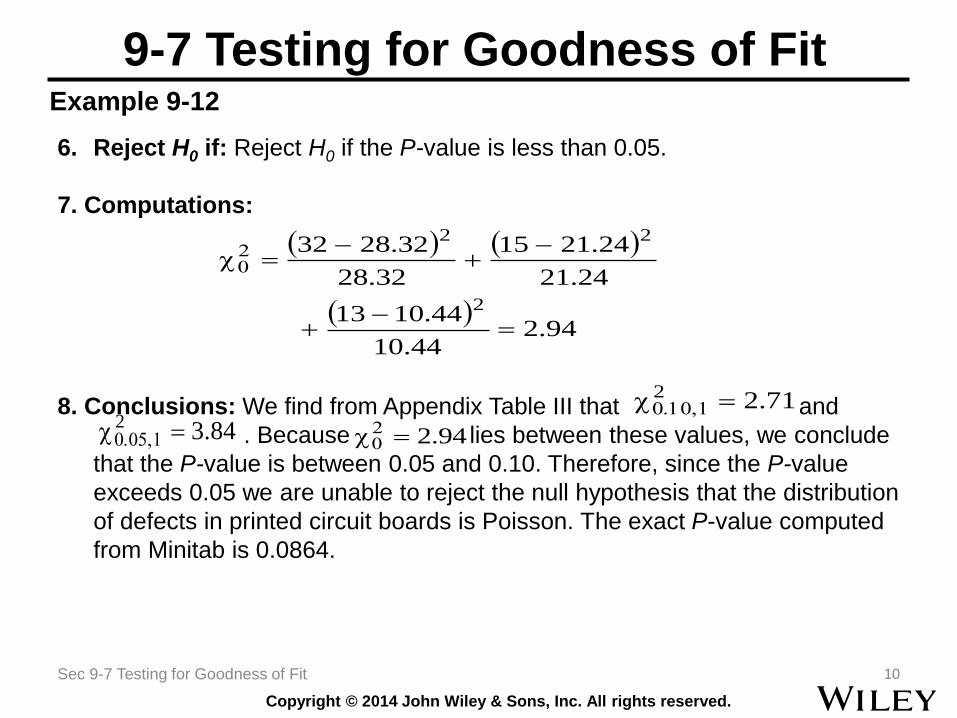
6. Reject H0 if: Reject H0 if the P-value is less than 0.05.

7. Computations:

8. Conclusions: We find from Appendix Table III that and

. Because lies between these values, we conclude

that the P-value is between 0.05 and 0.10. Therefore, since the P-value

exceeds 0.05 we are unable to reject the null hypothesis that the distribution

of defects in printed circuit boards is Poisson. The exact P-value computed

from Minitab is 0.0864.

94.2

44.10

44.1013

24.21

24.2115

32.28

32.2832

2

22

71.22 84.32 94.2


9-9 Nonparametric Procedures

11Sec 9-9 Nonparametric Procedures

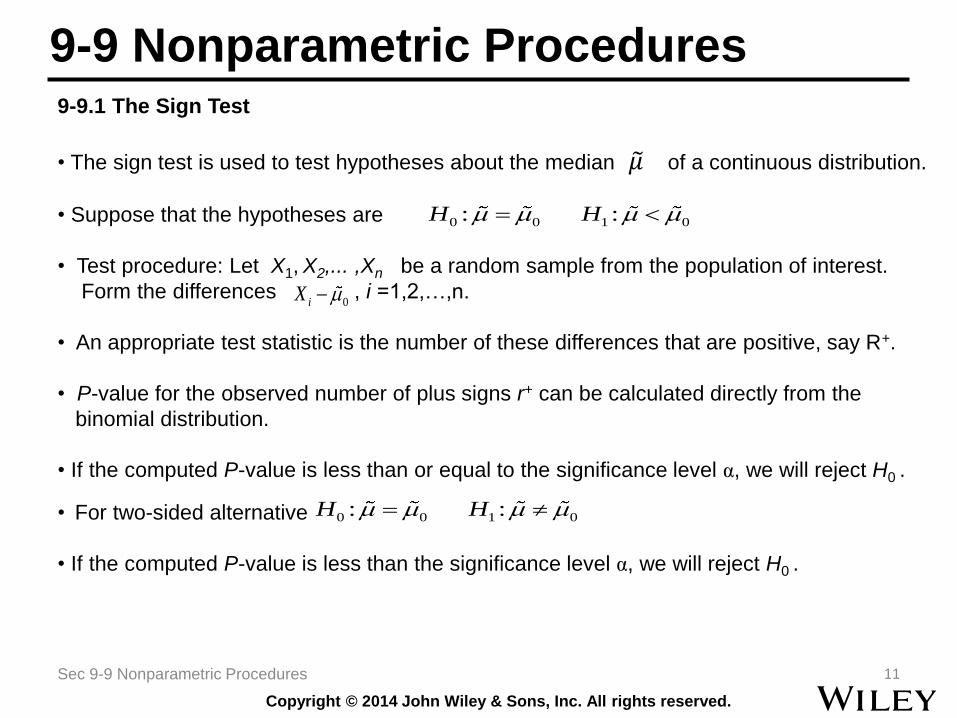
9-9.1 The Sign Test

• The sign test is used to test hypotheses about the median 𝜇 of a continuous distribution.

• Suppose that the hypotheses are

• Test procedure: Let X1, X2,... ,Xn be a random sample from the population of interest.

Form the differences , i =1,2,…,n.

• An appropriate test statistic is the number of these differences that are positive, say R+.

• P-value for the observed number of plus signs r+ can be calculated directly from the

binomial distribution.

• If the computed P-value is less than or equal to the significance level α, we will reject H0 .

• For two-sided alternative

• If the computed P-value is less than the significance level α, we will reject H0 .

0 0 1 0: :H H

0iX

0 0 1 0: :H H


12

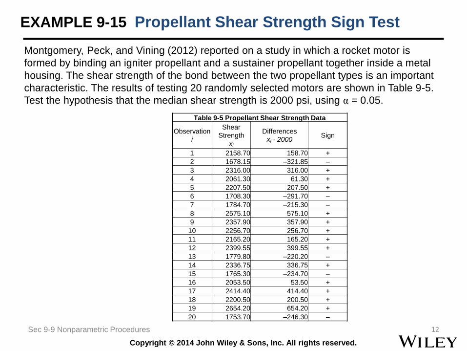
Montgomery, Peck, and Vining (2012) reported on a study in which a rocket motor is

formed by binding an igniter propellant and a sustainer propellant together inside a metal

housing. The shear strength of the bond between the two propellant types is an important

characteristic. The results of testing 20 randomly selected motors are shown in Table 9-5.

Test the hypothesis that the median shear strength is 2000 psi, using α = 0.05.

EXAMPLE 9-15 Propellant Shear Strength Sign Test

Table 9-5 Propellant Shear Strength Data

Observation

i

Shear

Strength

xi

Differences

xi - 2000Sign

1 2158.70 158.70 +

2 1678.15 –321.85 –

3 2316.00 316.00 +

4 2061.30 61.30 +

5 2207.50 207.50 +

6 1708.30 –291.70 –

7 1784.70 –215.30 –

8 2575.10 575.10 +

9 2357.90 357.90 +

10 2256.70 256.70 +

11 2165.20 165.20 +

12 2399.55 399.55 +

13 1779.80 –220.20 –

14 2336.75 336.75 +

15 1765.30 –234.70 –

16 2053.50 53.50 +

17 2414.40 414.40 +

18 2200.50 200.50 +

19 2654.20 654.20 +

20 1753.70 –246.30 –

Sec 9-9 Nonparametric Procedures


13

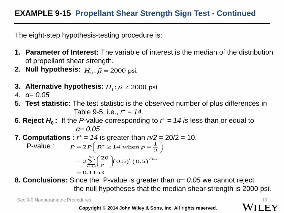
The eight-step hypothesis-testing procedure is:

1. Parameter of Interest: The variable of interest is the median of the distribution

of propellant shear strength.

2. Null hypothesis:

3. Alternative hypothesis:

4. α= 0.05

5. Test statistic: The test statistic is the observed number of plus differences in

Table 9-5, i.e., r+ = 14.

6. Reject H0 : If the P-value corresponding to r+ = 14 is less than or equal to

α= 0.05

7. Computations : r+ = 14 is greater than n/2 = 20/2 = 10.

P-value :

8. Conclusions: Since the P-value is greater than α= 0.05 we cannot reject

the null hypotheses that the median shear strength is 2000 psi.

EXAMPLE 9-15 Propellant Shear Strength Sign Test - Continued

0 : 2000 psiH

1 : 2000 psiH

20

20

14

12 14 when

2

202 0.5 0.5

0.1153

r r

r

P P R p

r



9-9 Nonparametric Procedures

14

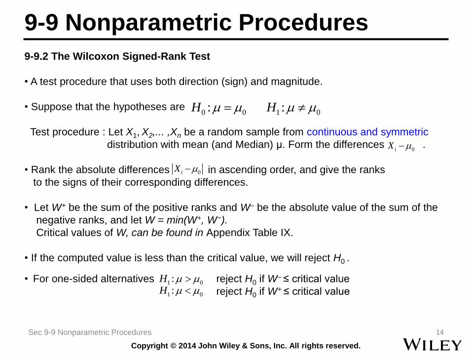
9-9.2 The Wilcoxon Signed-Rank Test

• A test procedure that uses both direction (sign) and magnitude.

• Suppose that the hypotheses are

Test procedure : Let X1, X2,... ,Xn be a random sample from continuous and symmetric

distribution with mean (and Median) μ. Form the differences .

• Rank the absolute differences in ascending order, and give the ranks

to the signs of their corresponding differences.

• Let W+ be the sum of the positive ranks and W– be the absolute value of the sum of the

negative ranks, and let W = min(W+, W−).

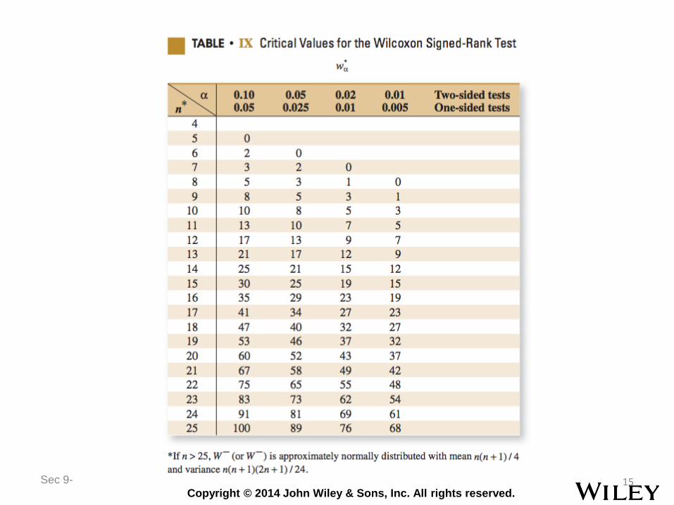
Critical values of W, can be found in Appendix Table IX.

• If the computed value is less than the critical value, we will reject H0 .

• For one-sided alternatives reject H0 if W– ≤ critical value

reject H0 if W+ ≤ critical value

0iX

0 0 1 0: :H H

0iX

1 0:H

1 0:H



Sec 9- 15


16

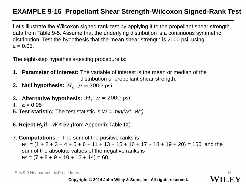
Let’s illustrate the Wilcoxon signed rank test by applying it to the propellant shear strength

data from Table 9-5. Assume that the underlying distribution is a continuous symmetric

distribution. Test the hypothesis that the mean shear strength is 2000 psi, using

α = 0.05.

The eight-step hypothesis-testing procedure is:

1. Parameter of Interest: The variable of interest is the mean or median of the

distribution of propellant shear strength.

2. Null hypothesis:

3. Alternative hypothesis:

4. α = 0.05

5. Test statistic: The test statistic is W = min(W+, W−)

6. Reject H0 if: W ≤ 52 (from Appendix Table IX).

7. Computations : The sum of the positive ranks is

w+ = (1 + 2 + 3 + 4 + 5 + 6 + 11 + 13 + 15 + 16 + 17 + 18 + 19 + 20) = 150, and the

sum of the absolute values of the negative ranks is

w- = (7 + 8 + 9 + 10 + 12 + 14) = 60.

EXAMPLE 9-16 Propellant Shear Strength-Wilcoxon Signed-Rank Test

0 : 2000 psiH

1 : 2000 psiH



17

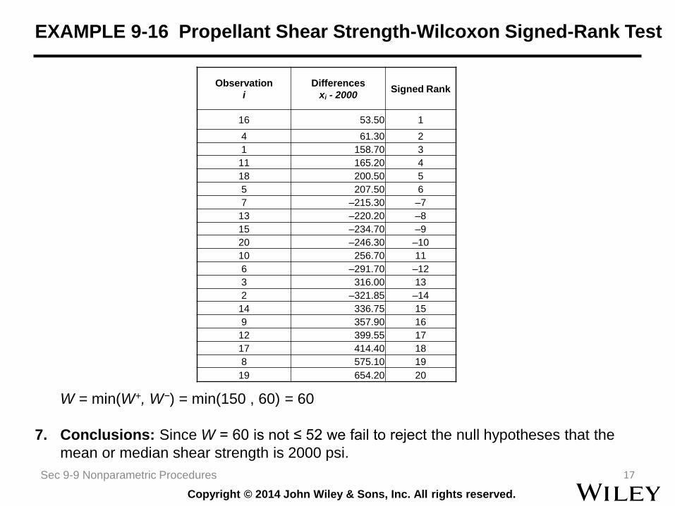
W = min(W+, W−) = min(150 , 60) = 60

7. Conclusions: Since W = 60 is not ≤ 52 we fail to reject the null hypotheses that the

mean or median shear strength is 2000 psi.

EXAMPLE 9-16 Propellant Shear Strength-Wilcoxon Signed-Rank Test

Observation

i

Differences

xi - 2000Signed Rank

16 53.50 1

4 61.30 2

1 158.70 3

11 165.20 4

18 200.50 5

5 207.50 6

7 –215.30 –7

13 –220.20 –8

15 –234.70 –9

20 –246.30 –10

10 256.70 11

6 –291.70 –12

3 316.00 13

2 –321.85 –14

14 336.75 15

9 357.90 16

12 399.55 17

17 414.40 18

8 575.10 19

19 654.20 20


Documents

Applied Statistics and Probability for Engineershaalshraideh/Courses/IE347/ch09.pdf · Applied Statistics and Probability for Engineers ... 9-9.3 Comparison to the t-test ... hypothesized