Embed Size (px)
Citation preview

2

Contents
1 Introduction 11
1.1 About This Book . . . . . . . . . . . . . . . . . . . . . . . . . . . . . . . . . . . . . . . . . . . 11
1.2 Conventions . . . . . . . . . . . . . . . . . . . . . . . . . . . . . . . . . . . . . . . . . . . . . . 11
1.3 Acknowledgements . . . . . . . . . . . . . . . . . . . . . . . . . . . . . . . . . . . . . . . . . . 12
1.4 License . . . . . . . . . . . . . . . . . . . . . . . . . . . . . . . . . . . . . . . . . . . . . . . . . 12
2 Introduction to R 13
2.1 Getting Started . . . . . . . . . . . . . . . . . . . . . . . . . . . . . . . . . . . . . . . . . . . . 13
2.2 Basic Calculations . . . . . . . . . . . . . . . . . . . . . . . . . . . . . . . . . . . . . . . . . . 14
2.3 Getting Help . . . . . . . . . . . . . . . . . . . . . . . . . . . . . . . . . . . . . . . . . . . . . 15
2.4 Installing Packages . . . . . . . . . . . . . . . . . . . . . . . . . . . . . . . . . . . . . . . . . . 15
3 Data and Programming 17
3.1 Data Types . . . . . . . . . . . . . . . . . . . . . . . . . . . . . . . . . . . . . . . . . . . . . . 17
3.2 Data Structures . . . . . . . . . . . . . . . . . . . . . . . . . . . . . . . . . . . . . . . . . . . . 17
3.2.1 Vectors . . . . . . . . . . . . . . . . . . . . . . . . . . . . . . . . . . . . . . . . . . . . 18
3.2.2 Vectorization . . . . . . . . . . . . . . . . . . . . . . . . . . . . . . . . . . . . . . . . . 21
3.2.3 Logical Operators . . . . . . . . . . . . . . . . . . . . . . . . . . . . . . . . . . . . . . 22
3.2.4 More Vectorization . . . . . . . . . . . . . . . . . . . . . . . . . . . . . . . . . . . . . . 23
3.2.5 Matrices . . . . . . . . . . . . . . . . . . . . . . . . . . . . . . . . . . . . . . . . . . . . 25
3.2.6 Lists . . . . . . . . . . . . . . . . . . . . . . . . . . . . . . . . . . . . . . . . . . . . . . 33
3.2.7 Data Frames . . . . . . . . . . . . . . . . . . . . . . . . . . . . . . . . . . . . . . . . . 35
3.3 Programming Basics . . . . . . . . . . . . . . . . . . . . . . . . . . . . . . . . . . . . . . . . . 41
3.3.1 Control Flow . . . . . . . . . . . . . . . . . . . . . . . . . . . . . . . . . . . . . . . . . 41
3.3.2 Functions . . . . . . . . . . . . . . . . . . . . . . . . . . . . . . . . . . . . . . . . . . . 42
3

4 CONTENTS
4 Summarizing Data 47
4.1 Summary Statistics . . . . . . . . . . . . . . . . . . . . . . . . . . . . . . . . . . . . . . . . . . 47
4.2 Plotting . . . . . . . . . . . . . . . . . . . . . . . . . . . . . . . . . . . . . . . . . . . . . . . . 48
4.2.1 Histograms . . . . . . . . . . . . . . . . . . . . . . . . . . . . . . . . . . . . . . . . . . 48
4.2.2 Barplots . . . . . . . . . . . . . . . . . . . . . . . . . . . . . . . . . . . . . . . . . . . . 50
4.2.3 Boxplots . . . . . . . . . . . . . . . . . . . . . . . . . . . . . . . . . . . . . . . . . . . . 52
4.2.4 Scatterplots . . . . . . . . . . . . . . . . . . . . . . . . . . . . . . . . . . . . . . . . . . 55
5 Probability and Statistics in R 59
5.1 Probability in R . . . . . . . . . . . . . . . . . . . . . . . . . . . . . . . . . . . . . . . . . . . . 59
5.1.1 Distributions . . . . . . . . . . . . . . . . . . . . . . . . . . . . . . . . . . . . . . . . . 59
5.2 Hypothesis Tests in R . . . . . . . . . . . . . . . . . . . . . . . . . . . . . . . . . . . . . . . . 60
5.2.1 One Sample t-Test: Review . . . . . . . . . . . . . . . . . . . . . . . . . . . . . . . . . 61
5.2.2 One Sample t-Test: Example . . . . . . . . . . . . . . . . . . . . . . . . . . . . . . . . 61
5.2.3 Two Sample t-Test: Review . . . . . . . . . . . . . . . . . . . . . . . . . . . . . . . . . 63
5.2.4 Two Sample t-Test: Example . . . . . . . . . . . . . . . . . . . . . . . . . . . . . . . . 64
5.3 Simulation . . . . . . . . . . . . . . . . . . . . . . . . . . . . . . . . . . . . . . . . . . . . . . . 66
5.3.1 Paired Differences . . . . . . . . . . . . . . . . . . . . . . . . . . . . . . . . . . . . . . 67
5.3.2 Distribution of a Sample Mean . . . . . . . . . . . . . . . . . . . . . . . . . . . . . . . 70
6 R Resources 73
6.1 Beginner Tutorials and References . . . . . . . . . . . . . . . . . . . . . . . . . . . . . . . . . 73
6.2 Intermediate References . . . . . . . . . . . . . . . . . . . . . . . . . . . . . . . . . . . . . . . 73
6.3 Advanced References . . . . . . . . . . . . . . . . . . . . . . . . . . . . . . . . . . . . . . . . . 74
6.4 Quick Comparisons to Other Languages . . . . . . . . . . . . . . . . . . . . . . . . . . . . . . 74
6.5 RStudio and RMarkdown Videos . . . . . . . . . . . . . . . . . . . . . . . . . . . . . . . . . . 74
6.6 RMarkdown Template . . . . . . . . . . . . . . . . . . . . . . . . . . . . . . . . . . . . . . . . 74
7 Simple Linear Regression 75
7.1 Modeling . . . . . . . . . . . . . . . . . . . . . . . . . . . . . . . . . . . . . . . . . . . . . . . 75
7.1.1 Simple Linear Regression Model . . . . . . . . . . . . . . . . . . . . . . . . . . . . . . 80
7.2 Least Squares Approach . . . . . . . . . . . . . . . . . . . . . . . . . . . . . . . . . . . . . . . 82
7.2.1 Making Predictions . . . . . . . . . . . . . . . . . . . . . . . . . . . . . . . . . . . . . . 84
7.2.2 Residuals . . . . . . . . . . . . . . . . . . . . . . . . . . . . . . . . . . . . . . . . . . . 86
7.2.3 Variance Estimation . . . . . . . . . . . . . . . . . . . . . . . . . . . . . . . . . . . . . 87
7.3 Decomposition of Variation . . . . . . . . . . . . . . . . . . . . . . . . . . . . . . . . . . . . . 88
7.3.1 Coefficient of Determination . . . . . . . . . . . . . . . . . . . . . . . . . . . . . . . . . 89
7.4 The lm Function . . . . . . . . . . . . . . . . . . . . . . . . . . . . . . . . . . . . . . . . . . . 91

CONTENTS 5
7.5 Maximum Likelihood Estimation (MLE) Approach . . . . . . . . . . . . . . . . . . . . . . . . 97
7.6 Simulating SLR . . . . . . . . . . . . . . . . . . . . . . . . . . . . . . . . . . . . . . . . . . . . 99
7.7 History . . . . . . . . . . . . . . . . . . . . . . . . . . . . . . . . . . . . . . . . . . . . . . . . 103
7.8 RMarkdown . . . . . . . . . . . . . . . . . . . . . . . . . . . . . . . . . . . . . . . . . . . . . . 103
8 Inference for Simple Linear Regression 105
8.1 Gauss–Markov Theorem . . . . . . . . . . . . . . . . . . . . . . . . . . . . . . . . . . . . . . . 108
8.2 Sampling Distributions . . . . . . . . . . . . . . . . . . . . . . . . . . . . . . . . . . . . . . . . 109
8.2.1 Simulating Sampling Distributions . . . . . . . . . . . . . . . . . . . . . . . . . . . . . 110
8.3 Standard Errors . . . . . . . . . . . . . . . . . . . . . . . . . . . . . . . . . . . . . . . . . . . . 115
8.4 Confidence Intervals for Slope and Intercept . . . . . . . . . . . . . . . . . . . . . . . . . . . . 118
8.5 Hypothesis Tests . . . . . . . . . . . . . . . . . . . . . . . . . . . . . . . . . . . . . . . . . . . 119
8.6 cars Example . . . . . . . . . . . . . . . . . . . . . . . . . . . . . . . . . . . . . . . . . . . . . 119
8.6.1 Tests in R . . . . . . . . . . . . . . . . . . . . . . . . . . . . . . . . . . . . . . . . . . . 120
8.6.2 Significance of Regression, t-Test . . . . . . . . . . . . . . . . . . . . . . . . . . . . . . 122
8.6.3 Confidence Intervals in R . . . . . . . . . . . . . . . . . . . . . . . . . . . . . . . . . . 123
8.7 Confidence Interval for Mean Response . . . . . . . . . . . . . . . . . . . . . . . . . . . . . . . 124
8.8 Prediction Interval for New Observations . . . . . . . . . . . . . . . . . . . . . . . . . . . . . . 126
8.9 Confidence and Prediction Bands . . . . . . . . . . . . . . . . . . . . . . . . . . . . . . . . . . 126
8.10 Significance of Regression, F-Test . . . . . . . . . . . . . . . . . . . . . . . . . . . . . . . . . . 128
9 Multiple Linear Regression 131
9.1 Matrix Approach to Regression . . . . . . . . . . . . . . . . . . . . . . . . . . . . . . . . . . . 135
9.2 Sampling Distribution . . . . . . . . . . . . . . . . . . . . . . . . . . . . . . . . . . . . . . . . 138
9.2.1 Single Parameter Tests . . . . . . . . . . . . . . . . . . . . . . . . . . . . . . . . . . . . 140
9.2.2 Confidence Intervals . . . . . . . . . . . . . . . . . . . . . . . . . . . . . . . . . . . . . 141
9.2.3 Confidence Intervals for Mean Response . . . . . . . . . . . . . . . . . . . . . . . . . . 141
9.2.4 Prediction Intervals . . . . . . . . . . . . . . . . . . . . . . . . . . . . . . . . . . . . . 144
9.3 Significance of Regression . . . . . . . . . . . . . . . . . . . . . . . . . . . . . . . . . . . . . . 145
9.4 Nested Models . . . . . . . . . . . . . . . . . . . . . . . . . . . . . . . . . . . . . . . . . . . . 148
9.5 Simulation . . . . . . . . . . . . . . . . . . . . . . . . . . . . . . . . . . . . . . . . . . . . . . . 151
10 Model Building 157
10.1 Family, Form, and Fit . . . . . . . . . . . . . . . . . . . . . . . . . . . . . . . . . . . . . . . . 157
10.1.1 Fit . . . . . . . . . . . . . . . . . . . . . . . . . . . . . . . . . . . . . . . . . . . . . . . 158
10.1.2 Form . . . . . . . . . . . . . . . . . . . . . . . . . . . . . . . . . . . . . . . . . . . . . . 158
10.1.3 Family . . . . . . . . . . . . . . . . . . . . . . . . . . . . . . . . . . . . . . . . . . . . . 159
10.1.4 Assumed Model, Fitted Model . . . . . . . . . . . . . . . . . . . . . . . . . . . . . . . 160

6 CONTENTS
10.2 Explanation versus Prediction . . . . . . . . . . . . . . . . . . . . . . . . . . . . . . . . . . . . 16010.2.1 Explanation . . . . . . . . . . . . . . . . . . . . . . . . . . . . . . . . . . . . . . . . . . 16010.2.2 Prediction . . . . . . . . . . . . . . . . . . . . . . . . . . . . . . . . . . . . . . . . . . . 162
10.3 Summary . . . . . . . . . . . . . . . . . . . . . . . . . . . . . . . . . . . . . . . . . . . . . . . 164
11 Categorical Predictors and Interactions 16511.1 Dummy Variables . . . . . . . . . . . . . . . . . . . . . . . . . . . . . . . . . . . . . . . . . . . 16511.2 Interactions . . . . . . . . . . . . . . . . . . . . . . . . . . . . . . . . . . . . . . . . . . . . . . 17211.3 Factor Variables . . . . . . . . . . . . . . . . . . . . . . . . . . . . . . . . . . . . . . . . . . . 179
11.3.1 Factors with More Than Two Levels . . . . . . . . . . . . . . . . . . . . . . . . . . . . 18211.4 Parameterization . . . . . . . . . . . . . . . . . . . . . . . . . . . . . . . . . . . . . . . . . . . 18711.5 Building Larger Models . . . . . . . . . . . . . . . . . . . . . . . . . . . . . . . . . . . . . . . 190
12 Analysis of Variance 19512.1 Experiments . . . . . . . . . . . . . . . . . . . . . . . . . . . . . . . . . . . . . . . . . . . . . . 19512.2 Two-Sample t-Test . . . . . . . . . . . . . . . . . . . . . . . . . . . . . . . . . . . . . . . . . . 19612.3 One-Way ANOVA . . . . . . . . . . . . . . . . . . . . . . . . . . . . . . . . . . . . . . . . . . 198
12.3.1 Factor Variables . . . . . . . . . . . . . . . . . . . . . . . . . . . . . . . . . . . . . . . 20412.3.2 Some Simulation . . . . . . . . . . . . . . . . . . . . . . . . . . . . . . . . . . . . . . . 20512.3.3 Power . . . . . . . . . . . . . . . . . . . . . . . . . . . . . . . . . . . . . . . . . . . . . 206
12.4 Post Hoc Testing . . . . . . . . . . . . . . . . . . . . . . . . . . . . . . . . . . . . . . . . . . . 20712.5 Two-Way ANOVA . . . . . . . . . . . . . . . . . . . . . . . . . . . . . . . . . . . . . . . . . . 21012.6 R Markdown . . . . . . . . . . . . . . . . . . . . . . . . . . . . . . . . . . . . . . . . . . . . . . 218
13 Model Diagnostics 21913.1 Model Assumptions . . . . . . . . . . . . . . . . . . . . . . . . . . . . . . . . . . . . . . . . . 21913.2 Checking Assumptions . . . . . . . . . . . . . . . . . . . . . . . . . . . . . . . . . . . . . . . . 221
13.2.1 Fitted versus Residuals Plot . . . . . . . . . . . . . . . . . . . . . . . . . . . . . . . . . 22213.2.2 Breusch-Pagan Test . . . . . . . . . . . . . . . . . . . . . . . . . . . . . . . . . . . . . 22713.2.3 Histograms . . . . . . . . . . . . . . . . . . . . . . . . . . . . . . . . . . . . . . . . . . 22813.2.4 Q-Q Plots . . . . . . . . . . . . . . . . . . . . . . . . . . . . . . . . . . . . . . . . . . . 22913.2.5 Shapiro-Wilk Test . . . . . . . . . . . . . . . . . . . . . . . . . . . . . . . . . . . . . . 236
13.3 Unusual Observations . . . . . . . . . . . . . . . . . . . . . . . . . . . . . . . . . . . . . . . . 23713.3.1 Leverage . . . . . . . . . . . . . . . . . . . . . . . . . . . . . . . . . . . . . . . . . . . . 23913.3.2 Outliers . . . . . . . . . . . . . . . . . . . . . . . . . . . . . . . . . . . . . . . . . . . . 24413.3.3 Influence . . . . . . . . . . . . . . . . . . . . . . . . . . . . . . . . . . . . . . . . . . . 246
13.4 Data Analysis Examples . . . . . . . . . . . . . . . . . . . . . . . . . . . . . . . . . . . . . . . 24713.4.1 Good Diagnostics . . . . . . . . . . . . . . . . . . . . . . . . . . . . . . . . . . . . . . . 24713.4.2 Suspect Diagnostics . . . . . . . . . . . . . . . . . . . . . . . . . . . . . . . . . . . . . 251

CONTENTS 7
14 Transformations 255
14.1 Response Transformation . . . . . . . . . . . . . . . . . . . . . . . . . . . . . . . . . . . . . . 255
14.1.1 Variance Stabilizing Transformations . . . . . . . . . . . . . . . . . . . . . . . . . . . . 258
14.1.2 Box-Cox Transformations . . . . . . . . . . . . . . . . . . . . . . . . . . . . . . . . . . 262
14.2 Predictor Transformation . . . . . . . . . . . . . . . . . . . . . . . . . . . . . . . . . . . . . . 269
14.2.1 Polynomials . . . . . . . . . . . . . . . . . . . . . . . . . . . . . . . . . . . . . . . . . . 272
14.2.2 A Quadratic Model . . . . . . . . . . . . . . . . . . . . . . . . . . . . . . . . . . . . . . 294
14.2.3 Overfitting and Extrapolation . . . . . . . . . . . . . . . . . . . . . . . . . . . . . . . . 299
14.2.4 Comparing Polynomial Models . . . . . . . . . . . . . . . . . . . . . . . . . . . . . . . 300
14.2.5 poly() Function and Orthogonal Polynomials . . . . . . . . . . . . . . . . . . . . . . . 304
14.2.6 Inhibit Function . . . . . . . . . . . . . . . . . . . . . . . . . . . . . . . . . . . . . . . 306
14.2.7 Data Example . . . . . . . . . . . . . . . . . . . . . . . . . . . . . . . . . . . . . . . . 307
15 Collinearity 315
15.1 Exact Collinearity . . . . . . . . . . . . . . . . . . . . . . . . . . . . . . . . . . . . . . . . . . 315
15.2 Collinearity . . . . . . . . . . . . . . . . . . . . . . . . . . . . . . . . . . . . . . . . . . . . . . 317
15.2.1 Variance Inflation Factor. . . . . . . . . . . . . . . . . . . . . . . . . . . . . . . . . . . 320
15.3 Simulation . . . . . . . . . . . . . . . . . . . . . . . . . . . . . . . . . . . . . . . . . . . . . . . 324
16 Variable Selection and Model Building 331
16.1 Quality Criterion . . . . . . . . . . . . . . . . . . . . . . . . . . . . . . . . . . . . . . . . . . . 331
16.1.1 Akaike Information Criterion . . . . . . . . . . . . . . . . . . . . . . . . . . . . . . . . 332
16.1.2 Bayesian Information Criterion . . . . . . . . . . . . . . . . . . . . . . . . . . . . . . . 333
16.1.3 Adjusted R-Squared . . . . . . . . . . . . . . . . . . . . . . . . . . . . . . . . . . . . . 333
16.1.4 Cross-Validated RMSE . . . . . . . . . . . . . . . . . . . . . . . . . . . . . . . . . . . 334
16.2 Selection Procedures . . . . . . . . . . . . . . . . . . . . . . . . . . . . . . . . . . . . . . . . . 337
16.2.1 Backward Search . . . . . . . . . . . . . . . . . . . . . . . . . . . . . . . . . . . . . . . 338
16.2.2 Forward Search . . . . . . . . . . . . . . . . . . . . . . . . . . . . . . . . . . . . . . . . 343
16.2.3 Stepwise Search . . . . . . . . . . . . . . . . . . . . . . . . . . . . . . . . . . . . . . . . 345
16.2.4 Exhaustive Search . . . . . . . . . . . . . . . . . . . . . . . . . . . . . . . . . . . . . . 348
16.3 Higher Order Terms . . . . . . . . . . . . . . . . . . . . . . . . . . . . . . . . . . . . . . . . . 352
16.4 Explanation versus Prediction . . . . . . . . . . . . . . . . . . . . . . . . . . . . . . . . . . . . 355
16.4.1 Explanation . . . . . . . . . . . . . . . . . . . . . . . . . . . . . . . . . . . . . . . . . . 356
16.4.2 Prediction . . . . . . . . . . . . . . . . . . . . . . . . . . . . . . . . . . . . . . . . . . . 357

8 CONTENTS
17 Logistic Regression 359
17.1 Generalized Linear Models . . . . . . . . . . . . . . . . . . . . . . . . . . . . . . . . . . . . . . 359
17.2 Binary Response . . . . . . . . . . . . . . . . . . . . . . . . . . . . . . . . . . . . . . . . . . . 360
17.2.1 Fitting Logistic Regression . . . . . . . . . . . . . . . . . . . . . . . . . . . . . . . . . 362
17.2.2 Simulation Examples . . . . . . . . . . . . . . . . . . . . . . . . . . . . . . . . . . . . . 363
17.3 Working with Logistic Regression . . . . . . . . . . . . . . . . . . . . . . . . . . . . . . . . . . 368
17.3.1 Testing with GLMs . . . . . . . . . . . . . . . . . . . . . . . . . . . . . . . . . . . . . . 369
17.3.2 Wald Test . . . . . . . . . . . . . . . . . . . . . . . . . . . . . . . . . . . . . . . . . . . 369
17.3.3 Likelihood-Ratio Test . . . . . . . . . . . . . . . . . . . . . . . . . . . . . . . . . . . . 369
17.3.4 SAheart Example . . . . . . . . . . . . . . . . . . . . . . . . . . . . . . . . . . . . . . 370
17.4 Classification . . . . . . . . . . . . . . . . . . . . . . . . . . . . . . . . . . . . . . . . . . . . . 376
17.4.1 spam Example . . . . . . . . . . . . . . . . . . . . . . . . . . . . . . . . . . . . . . . . 377
17.4.2 Evaluating Classifiers . . . . . . . . . . . . . . . . . . . . . . . . . . . . . . . . . . . . 379
18 Beyond 385
18.1 What’s Next . . . . . . . . . . . . . . . . . . . . . . . . . . . . . . . . . . . . . . . . . . . . . 385
18.2 RStudio . . . . . . . . . . . . . . . . . . . . . . . . . . . . . . . . . . . . . . . . . . . . . . . . 385
18.3 Tidy Data . . . . . . . . . . . . . . . . . . . . . . . . . . . . . . . . . . . . . . . . . . . . . . . 385
18.4 Visualization . . . . . . . . . . . . . . . . . . . . . . . . . . . . . . . . . . . . . . . . . . . . . 386
18.5 Web Applications . . . . . . . . . . . . . . . . . . . . . . . . . . . . . . . . . . . . . . . . . . . 386
18.6 Experimental Design . . . . . . . . . . . . . . . . . . . . . . . . . . . . . . . . . . . . . . . . . 386
18.7 Machine Learning . . . . . . . . . . . . . . . . . . . . . . . . . . . . . . . . . . . . . . . . . . . 386
18.7.1 Deep Learning . . . . . . . . . . . . . . . . . . . . . . . . . . . . . . . . . . . . . . . . 386
18.8 Time Series . . . . . . . . . . . . . . . . . . . . . . . . . . . . . . . . . . . . . . . . . . . . . . 386
18.9 Bayesianism . . . . . . . . . . . . . . . . . . . . . . . . . . . . . . . . . . . . . . . . . . . . . . 387
18.10High Performance Computing . . . . . . . . . . . . . . . . . . . . . . . . . . . . . . . . . . . . 387
18.11Further R Resources . . . . . . . . . . . . . . . . . . . . . . . . . . . . . . . . . . . . . . . . . 387
19 Appendix 389
## [[1]]## NULL#### [[2]]## NULL#### [[3]]## NULL#### [[4]]## NULL

CONTENTS 9
#### [[5]]## NULL#### [[6]]## NULL#### [[7]]## NULL#### [[8]]## NULL#### [[9]]## NULL#### [[10]]## NULL#### [[11]]## NULL

10 CONTENTS

Chapter 1
Introduction
Welcome to Applied Statistics with R!
1.1 About This Book
This book was originally (and currently) designed for use with STAT 420, Methods of Applied Statistics, atthe University of Illinois at Urbana-Champaign. It may certainly be used elsewhere, but any references to“this course” in this book specifically refer to STAT 420.This book is under active development. When possible, it would be best to always access the text online tobe sure you are using the most up-to-date version. Also, the html version provides additional features suchas changing text size, font, and colors. If you are in need of a local copy, a pdf version is continuouslymaintained.Since this book is under active development you may encounter errors ranging from typos, to broken code,to poorly explained topics. If you do, please let us know! Simply send an email and we will make the changesas soon as possible. (dalpiaz2 AT illinois DOT edu) Or, if you know RMarkdown and are familiar withGitHub, make a pull request and fix an issue yourself! This process is partially automated by the edit buttonin the top-left corner of the html version. If your suggestion or fix becomes part of the book, you will beadded to the list at the end of this chapter. We’ll also link to your GitHub account, or personal websiteupon request.This text uses MathJax to render mathematical notation for the web. Occasionally, but rarely, a JavaScripterror will prevent MathJax from rendering correctly. In this case, you will see the “code” instead of theexpected mathematical equations. From experience, this is almost always fixed by simply refreshing thepage. You’ll also notice that if you right-click any equation you can obtain the MathML Code (for copyinginto Microsoft Word) or the TeX command used to generate the equation.
a2 + b2 = c2
1.2 Conventions
R code will be typeset using a monospace font which is syntax highlighted.
a = 3b = 4sqrt(a ^ 2 + b ^ 2)
11

12 CHAPTER 1. INTRODUCTION
R output lines, which would appear in the console will begin with ##. They will generally not be syntaxhighlighted.
## [1] 5
We use the quantity p to refer to the number of β parameters in a linear model, not the number of predictors.
1.3 Acknowledgements
Material in this book was heavily influenced by:
• Alex Stepanov
– Longtime instructor of STAT 420 at the University of Illinois at Urbana-Champaign. The authorof this book actually took Alex’s STAT 420 class many years ago! Alex provided or inspired manyof the examples in the text.
• David Unger
– Another STAT 420 instructor at the University of Illinois at Urbana-Champaign. Co-taught withthe author during the summer of 2016 while this book was first being developed. Provided endlesshours of copy editing and countless suggestions.
• James Balamuta
– Current graduate student at the University of Illinois at Urbana-Champaign. Provided the initialpush to write this book by introducing the author to the bookdown package in R. Also a frequentcontributor via GitHub.
Your name could be here! Suggest an edit! Correct a typo! If you submit a correction and would like to belisted below, please provide your name as you would like it to appear, as well as a link to a GitHub, LinkedIn,or personal website.
• Daniel McQuillan• Mason Rubenstein• Yuhang Wang• Zhao Liu• Jinfeng Xiao• Somu Palaniappan• Michael Hung-Yiu Chan• Eloise Rosen• Kiomars Nassiri
1.4 License
Figure 1.1: This work is licensed under a Creative Commons Attribution-NonCommercial-ShareAlike 4.0International License.
Chapter 2
Introduction to R
2.1 Getting Started
R is both a programming language and software environment for statistical computing, which is free andopen-source. To get started, you will need to install two pieces of software:
• R, the actual programming language.– Chose your operating system, and select the most recent version, 3.5.0.
• RStudio, an excellent IDE for working with R.– Note, you must have R installed to use RStudio. RStudio is simply an interface used to interact
with R.
The popularity of R is on the rise, and everyday it becomes a better tool for statistical analysis. It evengenerated this book! (A skill you will learn in this course.) There are many good resources for learning R.The following few chapters will serve as a whirlwind introduction to R. They are by no means meant to be acomplete reference for the R language, but simply an introduction to the basics that we will need along theway. Several of the more important topics will be re-stressed as they are actually needed for analyses.These introductory R chapters may feel like an overwhelming amount of information. You are not expectedto pick up everything the first time through. You should try all of the code from these chapters, then returnto them a number of times as you return to the concepts when performing analyses.R is used both for software development and data analysis. We will operate in a grey area, somewherebetween these two tasks. Our main goal will be to analyze data, but we will also perform programmingexercises that help illustrate certain concepts.RStudio has a large number of useful keyboard shortcuts. A list of these can be found using a keyboardshortcut – the keyboard shortcut to rule them all:
• On Windows: Alt + Shift + K• On Mac: Option + Shift + K
The RStudio team has developed a number of “cheatsheets” for working with both R and RStudio. Thisparticular cheatseet for Base R will summarize many of the concepts in this document.When programming, it is often a good practice to follow a style guide. (Where do spaces go? Tabs or spaces?Underscores or CamelCase when naming variables?) No style guide is “correct” but it helps to be aware ofwhat others do. The more import thing is to be consistent within your own code.
13

14 CHAPTER 2. INTRODUCTION TO R
• Hadley Wickham Style Guide from Advanced R• Google Style Guide
For this course, our main deviation from these two guides is the use of = in place of <-. (More on that later.)
2.2 Basic Calculations
To get started, we’ll use R like a simple calculator.
Addition, Subtraction, Multiplication and Division
Math R Result3 + 2 3 + 2 53 − 2 3 - 2 13 · 2 3 * 2 63/2 3 / 2 1.5
Exponents
Math R Result32 3 ^ 2 92(−3) 2 ^ (-3) 0.1251001/2 100 ^ (1 / 2) 10√
100 sqrt(100) 10
Mathematical Constants
Math R Resultπ pi 3.1415927e exp(1) 2.7182818
Logarithms
Note that we will use ln and log interchangeably to mean the natural logarithm. There is no ln() in R,instead it uses log() to mean the natural logarithm.
Math R Resultlog(e) log(exp(1)) 1log10(1000) log10(1000) 3log2(8) log2(8) 3log4(16) log(16, base = 4) 2
Trigonometry

2.3. GETTING HELP 15
Math R Resultsin(π/2) sin(pi / 2) 1cos(0) cos(0) 1
2.3 Getting Help
In using R as a calculator, we have seen a number of functions: sqrt(), exp(), log() and sin(). To getdocumentation about a function in R, simply put a question mark in front of the function name and RStudiowill display the documentation, for example:
?log?sin?paste?lm
Frequently one of the most difficult things to do when learning R is asking for help. First, you need to decideto ask for help, then you need to know how to ask for help. Your very first line of defense should be toGoogle your error message or a short description of your issue. (The ability to solve problems using thismethod is quickly becoming an extremely valuable skill.) If that fails, and it eventually will, you should askfor help. There are a number of things you should include when emailing an instructor, or posting to a helpwebsite such as Stack Exchange.
• Describe what you expect the code to do.• State the end goal you are trying to achieve. (Sometimes what you expect the code to do, is not what
you want to actually do.)• Provide the full text of any errors you have received.• Provide enough code to recreate the error. Often for the purpose of this course, you could simply email
your entire .R or .Rmd file.• Sometimes it is also helpful to include a screenshot of your entire RStudio window when the error
occurs.
If you follow these steps, you will get your issue resolved much quicker, and possibly learn more in the process.Do not be discouraged by running into errors and difficulties when learning R. (Or any technical skill.) It issimply part of the learning process.
2.4 Installing Packages
R comes with a number of built-in functions and datasets, but one of the main strengths of R as an open-source project is its package system. Packages add additional functions and data. Frequently if you want todo something in R, and it is not available by default, there is a good chance that there is a package that willfulfill your needs.
To install a package, use the install.packages() function. Think of this as buying a recipe book from thestore, bringing it home, and putting it on your shelf.
install.packages("ggplot2")
Once a package is installed, it must be loaded into your current R session before being used. Think of thisas taking the book off of the shelf and opening it up to read.

16 CHAPTER 2. INTRODUCTION TO R
library(ggplot2)
Once you close R, all the packages are closed and put back on the imaginary shelf. The next time you openR, you do not have to install the package again, but you do have to load any packages you intend to use byinvoking library().

Chapter 3
Data and Programming
3.1 Data Types
R has a number of basic data types.
• Numeric
– Also known as Double. The default type when dealing with numbers.– Examples: 1, 1.0, 42.5
• Integer
– Examples: 1L, 2L, 42L
• Complex
– Example: 4 + 2i
• Logical
– Two possible values: TRUE and FALSE– You can also use T and F, but this is not recommended.– NA is also considered logical.
• Character
– Examples: "a", "Statistics", "1 plus 2."
3.2 Data Structures
R also has a number of basic data structures. A data structure is either homogeneous (all elements are ofthe same data type) or heterogeneous (elements can be of more than one data type).
Dimension Homogeneous Heterogeneous1 Vector List2 Matrix Data Frame3+ Array
17

18 CHAPTER 3. DATA AND PROGRAMMING
3.2.1 Vectors
Many operations in R make heavy use of vectors. Vectors in R are indexed starting at 1. That is what the[1] in the output is indicating, that the first element of the row being displayed is the first element of thevector. Larger vectors will start additional rows with [*] where * is the index of the first element of therow.
Possibly the most common way to create a vector in R is using the c() function, which is short for “combine.””As the name suggests, it combines a list of elements separated by commas.
c(1, 3, 5, 7, 8, 9)
## [1] 1 3 5 7 8 9
Here R simply outputs this vector. If we would like to store this vector in a variable we can do so with theassignment operator =. In this case the variable x now holds the vector we just created, and we can accessthe vector by typing x.
x = c(1, 3, 5, 7, 8, 9)x
## [1] 1 3 5 7 8 9
As an aside, there is a long history of the assignment operator in R, partially due to the keys available onthe keyboards of the creators of the S language. (Which preceded R.) For simplicity we will use =, but knowthat often you will see <- as the assignment operator.
The pros and cons of these two are well beyond the scope of this book, but know that for our purposes youwill have no issue if you simply use =. If you are interested in the weird cases where the difference matters,check out The R Inferno.
If you wish to use <-, you will still need to use =, however only for argument passing. Some users like to keepassignment (<-) and argument passing (=) separate. No matter what you choose, the more important thingis that you stay consistent. Also, if working on a larger collaborative project, you should use whateverstyle is already in place.
Because vectors must contains elements that are all the same type, R will automatically coerce to a singletype when attempting to create a vector that combines multiple types.
c(42, "Statistics", TRUE)
## [1] "42" "Statistics" "TRUE"
c(42, TRUE)
## [1] 42 1
Frequently you may wish to create a vector based on a sequence of numbers. The quickest and easiest wayto do this is with the : operator, which creates a sequence of integers between two specified integers.
(y = 1:100)

3.2. DATA STRUCTURES 19
## [1] 1 2 3 4 5 6 7 8 9 10 11 12 13 14 15 16 17 18## [19] 19 20 21 22 23 24 25 26 27 28 29 30 31 32 33 34 35 36## [37] 37 38 39 40 41 42 43 44 45 46 47 48 49 50 51 52 53 54## [55] 55 56 57 58 59 60 61 62 63 64 65 66 67 68 69 70 71 72## [73] 73 74 75 76 77 78 79 80 81 82 83 84 85 86 87 88 89 90## [91] 91 92 93 94 95 96 97 98 99 100
Here we see R labeling the rows after the first since this is a large vector. Also, we see that by puttingparentheses around the assignment, R both stores the vector in a variable called y and automatically outputsy to the console.Note that scalars do not exists in R. They are simply vectors of length 1.
2
## [1] 2
If we want to create a sequence that isn’t limited to integers and increasing by 1 at a time, we can use theseq() function.
seq(from = 1.5, to = 4.2, by = 0.1)
## [1] 1.5 1.6 1.7 1.8 1.9 2.0 2.1 2.2 2.3 2.4 2.5 2.6 2.7 2.8 2.9 3.0 3.1 3.2 3.3## [20] 3.4 3.5 3.6 3.7 3.8 3.9 4.0 4.1 4.2
We will discuss functions in detail later, but note here that the input labels from, to, and by are optional.
seq(1.5, 4.2, 0.1)
## [1] 1.5 1.6 1.7 1.8 1.9 2.0 2.1 2.2 2.3 2.4 2.5 2.6 2.7 2.8 2.9 3.0 3.1 3.2 3.3## [20] 3.4 3.5 3.6 3.7 3.8 3.9 4.0 4.1 4.2
Another common operation to create a vector is rep(), which can repeat a single value a number of times.
rep("A", times = 10)
## [1] "A" "A" "A" "A" "A" "A" "A" "A" "A" "A"
The rep() function can be used to repeat a vector some number of times.
rep(x, times = 3)
## [1] 1 3 5 7 8 9 1 3 5 7 8 9 1 3 5 7 8 9
We have now seen four different ways to create vectors:
• c()• :• seq()• rep()
So far we have mostly used them in isolation, but they are often used together.

20 CHAPTER 3. DATA AND PROGRAMMING
c(x, rep(seq(1, 9, 2), 3), c(1, 2, 3), 42, 2:4)
## [1] 1 3 5 7 8 9 1 3 5 7 9 1 3 5 7 9 1 3 5 7 9 1 2 3 42## [26] 2 3 4
The length of a vector can be obtained with the length() function.
length(x)
## [1] 6
length(y)
## [1] 100
3.2.1.1 Subsetting
To subset a vector, we use square brackets, [].
x
## [1] 1 3 5 7 8 9
x[1]
## [1] 1
x[3]
## [1] 5
We see that x[1] returns the first element, and x[3] returns the third element.
x[-2]
## [1] 1 5 7 8 9
We can also exclude certain indexes, in this case the second element.
x[1:3]
## [1] 1 3 5
x[c(1,3,4)]
## [1] 1 5 7
Lastly we see that we can subset based on a vector of indices.All of the above are subsetting a vector using a vector of indexes. (Remember a single number is still avector.) We could instead use a vector of logical values.

3.2. DATA STRUCTURES 21
z = c(TRUE, TRUE, FALSE, TRUE, TRUE, FALSE)z
## [1] TRUE TRUE FALSE TRUE TRUE FALSE
x[z]
## [1] 1 3 7 8
3.2.2 Vectorization
One of the biggest strengths of R is its use of vectorized operations. (Frequently the lack of understandingof this concept leads of a belief that R is slow. R is not the fastest language, but it has a reputation for beingslower than it really is.)
x = 1:10x + 1
## [1] 2 3 4 5 6 7 8 9 10 11
2 * x
## [1] 2 4 6 8 10 12 14 16 18 20
2 ^ x
## [1] 2 4 8 16 32 64 128 256 512 1024
sqrt(x)
## [1] 1.000000 1.414214 1.732051 2.000000 2.236068 2.449490 2.645751 2.828427## [9] 3.000000 3.162278
log(x)
## [1] 0.0000000 0.6931472 1.0986123 1.3862944 1.6094379 1.7917595 1.9459101## [8] 2.0794415 2.1972246 2.3025851
We see that when a function like log() is called on a vector x, a vector is returned which has applied thefunction to each element of the vector x.

22 CHAPTER 3. DATA AND PROGRAMMING
Operator Summary Example Result
3.2.3 Logical Operators
Operator Summary Example Resultx < y x less than y 3 < 42 TRUEx > y x greater than y 3 > 42 FALSEx <= y x less than or equal to y 3 <= 42 TRUEx >= y x greater than or equal to y 3 >= 42 FALSEx == y xequal to y 3 == 42 FALSEx != y x not equal to y 3 != 42 TRUE!x not x !(3 > 42) TRUEx | y x or y (3 > 42) | TRUE TRUEx & y x and y (3 < 4) & ( 42 > 13) TRUE
In R, logical operators are vectorized.
x = c(1, 3, 5, 7, 8, 9)
x > 3
## [1] FALSE FALSE TRUE TRUE TRUE TRUE
x < 3
## [1] TRUE FALSE FALSE FALSE FALSE FALSE
x == 3
## [1] FALSE TRUE FALSE FALSE FALSE FALSE
x != 3
## [1] TRUE FALSE TRUE TRUE TRUE TRUE
x == 3 & x != 3
## [1] FALSE FALSE FALSE FALSE FALSE FALSE
x == 3 | x != 3
## [1] TRUE TRUE TRUE TRUE TRUE TRUE
This is extremely useful for subsetting.

3.2. DATA STRUCTURES 23
x[x > 3]
## [1] 5 7 8 9
x[x != 3]
## [1] 1 5 7 8 9
• TODO: coercion
sum(x > 3)
## [1] 4
as.numeric(x > 3)
## [1] 0 0 1 1 1 1
Here we see that using the sum() function on a vector of logical TRUE and FALSE values that is the result ofx > 3 results in a numeric result. R is first automatically coercing the logical to numeric where TRUE is 1and FALSE is 0. This coercion from logical to numeric happens for most mathematical operations.
which(x > 3)
## [1] 3 4 5 6
x[which(x > 3)]
## [1] 5 7 8 9
max(x)
## [1] 9
which(x == max(x))
## [1] 6
which.max(x)
## [1] 6
3.2.4 More Vectorization

24 CHAPTER 3. DATA AND PROGRAMMING
x = c(1, 3, 5, 7, 8, 9)y = 1:100
x + 2
## [1] 3 5 7 9 10 11
x + rep(2, 6)
## [1] 3 5 7 9 10 11
x > 3
## [1] FALSE FALSE TRUE TRUE TRUE TRUE
x > rep(3, 6)
## [1] FALSE FALSE TRUE TRUE TRUE TRUE
x + y
## Warning in x + y: longer object length is not a multiple of shorter object## length
## [1] 2 5 8 11 13 15 8 11 14 17 19 21 14 17 20 23 25 27## [19] 20 23 26 29 31 33 26 29 32 35 37 39 32 35 38 41 43 45## [37] 38 41 44 47 49 51 44 47 50 53 55 57 50 53 56 59 61 63## [55] 56 59 62 65 67 69 62 65 68 71 73 75 68 71 74 77 79 81## [73] 74 77 80 83 85 87 80 83 86 89 91 93 86 89 92 95 97 99## [91] 92 95 98 101 103 105 98 101 104 107
length(x)
## [1] 6
length(y)
## [1] 100
length(y) / length(x)
## [1] 16.66667
(x + y) - y
## Warning in x + y: longer object length is not a multiple of shorter object## length
## [1] 1 3 5 7 8 9 1 3 5 7 8 9 1 3 5 7 8 9 1 3 5 7 8 9 1 3 5 7 8 9 1 3 5 7 8 9 1## [38] 3 5 7 8 9 1 3 5 7 8 9 1 3 5 7 8 9 1 3 5 7 8 9 1 3 5 7 8 9 1 3 5 7 8 9 1 3## [75] 5 7 8 9 1 3 5 7 8 9 1 3 5 7 8 9 1 3 5 7 8 9 1 3 5 7

3.2. DATA STRUCTURES 25
y = 1:60x + y
## [1] 2 5 8 11 13 15 8 11 14 17 19 21 14 17 20 23 25 27 20 23 26 29 31 33 26## [26] 29 32 35 37 39 32 35 38 41 43 45 38 41 44 47 49 51 44 47 50 53 55 57 50 53## [51] 56 59 61 63 56 59 62 65 67 69
length(y) / length(x)
## [1] 10
rep(x, 10) + y
## [1] 2 5 8 11 13 15 8 11 14 17 19 21 14 17 20 23 25 27 20 23 26 29 31 33 26## [26] 29 32 35 37 39 32 35 38 41 43 45 38 41 44 47 49 51 44 47 50 53 55 57 50 53## [51] 56 59 61 63 56 59 62 65 67 69
all(x + y == rep(x, 10) + y)
## [1] TRUE
identical(x + y, rep(x, 10) + y)
## [1] TRUE
# ?any# ?all.equal
3.2.5 Matrices
R can also be used for matrix calculations. Matrices have rows and columns containing a single data type.In a matrix, the order of rows and columns is important. (This is not true of data frames, which we will seelater.)
Matrices can be created using the matrix function.
x = 1:9x
## [1] 1 2 3 4 5 6 7 8 9
X = matrix(x, nrow = 3, ncol = 3)X
## [,1] [,2] [,3]## [1,] 1 4 7## [2,] 2 5 8## [3,] 3 6 9

26 CHAPTER 3. DATA AND PROGRAMMING
Note here that we are using two different variables: lower case x, which stores a vector and capital X, whichstores a matrix. (Following the usual mathematical convention.) We can do this because R is case sensitive.
By default the matrix function reorders a vector into columns, but we can also tell R to use rows instead.
Y = matrix(x, nrow = 3, ncol = 3, byrow = TRUE)Y
## [,1] [,2] [,3]## [1,] 1 2 3## [2,] 4 5 6## [3,] 7 8 9
We can also create a matrix of a specified dimension where every element is the same, in this case 0.
Z = matrix(0, 2, 4)Z
## [,1] [,2] [,3] [,4]## [1,] 0 0 0 0## [2,] 0 0 0 0
Like vectors, matrices can be subsetted using square brackets, []. However, since matrices are two-dimensional, we need to specify both a row and a column when subsetting.
X
## [,1] [,2] [,3]## [1,] 1 4 7## [2,] 2 5 8## [3,] 3 6 9
X[1, 2]
## [1] 4
Here we accessed the element in the first row and the second column. We could also subset an entire row orcolumn.
X[1, ]
## [1] 1 4 7
X[, 2]
## [1] 4 5 6
We can also use vectors to subset more than one row or column at a time. Here we subset to the first andthird column of the second row.

3.2. DATA STRUCTURES 27
X[2, c(1, 3)]
## [1] 2 8
Matrices can also be created by combining vectors as columns, using cbind, or combining vectors as rows,using rbind.
x = 1:9rev(x)
## [1] 9 8 7 6 5 4 3 2 1
rep(1, 9)
## [1] 1 1 1 1 1 1 1 1 1
rbind(x, rev(x), rep(1, 9))
## [,1] [,2] [,3] [,4] [,5] [,6] [,7] [,8] [,9]## x 1 2 3 4 5 6 7 8 9## 9 8 7 6 5 4 3 2 1## 1 1 1 1 1 1 1 1 1
cbind(col_1 = x, col_2 = rev(x), col_3 = rep(1, 9))
## col_1 col_2 col_3## [1,] 1 9 1## [2,] 2 8 1## [3,] 3 7 1## [4,] 4 6 1## [5,] 5 5 1## [6,] 6 4 1## [7,] 7 3 1## [8,] 8 2 1## [9,] 9 1 1
When using rbind and cbind you can specify “argument” names that will be used as column names.R can then be used to perform matrix calculations.
x = 1:9y = 9:1X = matrix(x, 3, 3)Y = matrix(y, 3, 3)X
## [,1] [,2] [,3]## [1,] 1 4 7## [2,] 2 5 8## [3,] 3 6 9

28 CHAPTER 3. DATA AND PROGRAMMING
Y
## [,1] [,2] [,3]## [1,] 9 6 3## [2,] 8 5 2## [3,] 7 4 1
X + Y
## [,1] [,2] [,3]## [1,] 10 10 10## [2,] 10 10 10## [3,] 10 10 10
X - Y
## [,1] [,2] [,3]## [1,] -8 -2 4## [2,] -6 0 6## [3,] -4 2 8
X * Y
## [,1] [,2] [,3]## [1,] 9 24 21## [2,] 16 25 16## [3,] 21 24 9
X / Y
## [,1] [,2] [,3]## [1,] 0.1111111 0.6666667 2.333333## [2,] 0.2500000 1.0000000 4.000000## [3,] 0.4285714 1.5000000 9.000000
Note that X * Y is not matrix multiplication. It is element by element multiplication. (Same for X / Y).Instead, matrix multiplication uses %*%. Other matrix functions include t() which gives the transpose of amatrix and solve() which returns the inverse of a square matrix if it is invertible.
X %*% Y
## [,1] [,2] [,3]## [1,] 90 54 18## [2,] 114 69 24## [3,] 138 84 30
t(X)
## [,1] [,2] [,3]## [1,] 1 2 3## [2,] 4 5 6## [3,] 7 8 9

3.2. DATA STRUCTURES 29
Z = matrix(c(9, 2, -3, 2, 4, -2, -3, -2, 16), 3, byrow = TRUE)Z
## [,1] [,2] [,3]## [1,] 9 2 -3## [2,] 2 4 -2## [3,] -3 -2 16
solve(Z)
## [,1] [,2] [,3]## [1,] 0.12931034 -0.05603448 0.01724138## [2,] -0.05603448 0.29094828 0.02586207## [3,] 0.01724138 0.02586207 0.06896552
To verify that solve(Z) returns the inverse, we multiply it by Z. We would expect this to return the identitymatrix, however we see that this is not the case due to some computational issues. However, R also hasthe all.equal() function which checks for equality, with some small tolerance which accounts for somecomputational issues. The identical() function is used to check for exact equality.
solve(Z) %*% Z
## [,1] [,2] [,3]## [1,] 1.000000e+00 -6.245005e-17 0.000000e+00## [2,] 8.326673e-17 1.000000e+00 5.551115e-17## [3,] 2.775558e-17 0.000000e+00 1.000000e+00
diag(3)
## [,1] [,2] [,3]## [1,] 1 0 0## [2,] 0 1 0## [3,] 0 0 1
all.equal(solve(Z) %*% Z, diag(3))
## [1] TRUE
R has a number of matrix specific functions for obtaining dimension and summary information.
X = matrix(1:6, 2, 3)X
## [,1] [,2] [,3]## [1,] 1 3 5## [2,] 2 4 6

30 CHAPTER 3. DATA AND PROGRAMMING
dim(X)
## [1] 2 3
rowSums(X)
## [1] 9 12
colSums(X)
## [1] 3 7 11
rowMeans(X)
## [1] 3 4
colMeans(X)
## [1] 1.5 3.5 5.5
The diag() function can be used in a number of ways. We can extract the diagonal of a matrix.
diag(Z)
## [1] 9 4 16
Or create a matrix with specified elements on the diagonal. (And 0 on the off-diagonals.)
diag(1:5)
## [,1] [,2] [,3] [,4] [,5]## [1,] 1 0 0 0 0## [2,] 0 2 0 0 0## [3,] 0 0 3 0 0## [4,] 0 0 0 4 0## [5,] 0 0 0 0 5
Or, lastly, create a square matrix of a certain dimension with 1 for every element of the diagonal and 0 forthe off-diagonals.
diag(5)
## [,1] [,2] [,3] [,4] [,5]## [1,] 1 0 0 0 0## [2,] 0 1 0 0 0## [3,] 0 0 1 0 0## [4,] 0 0 0 1 0## [5,] 0 0 0 0 1
3.2. DATA STRUCTURES 31
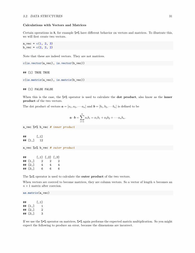
Calculations with Vectors and Matrices
Certain operations in R, for example %*% have different behavior on vectors and matrices. To illustrate this,we will first create two vectors.
a_vec = c(1, 2, 3)b_vec = c(2, 2, 2)
Note that these are indeed vectors. They are not matrices.
c(is.vector(a_vec), is.vector(b_vec))
## [1] TRUE TRUE
c(is.matrix(a_vec), is.matrix(b_vec))
## [1] FALSE FALSE
When this is the case, the %*% operator is used to calculate the dot product, also know as the innerproduct of the two vectors.The dot product of vectors a = [a1, a2, · · · an] and b = [b1, b2, · · · bn] is defined to be
a · b =n∑
i=1aibi = a1b1 + a2b2 + · · · anbn.
a_vec %*% b_vec # inner product
## [,1]## [1,] 12
a_vec %o% b_vec # outer product
## [,1] [,2] [,3]## [1,] 2 2 2## [2,] 4 4 4## [3,] 6 6 6
The %o% operator is used to calculate the outer product of the two vectors.When vectors are coerced to become matrices, they are column vectors. So a vector of length n becomes ann × 1 matrix after coercion.
as.matrix(a_vec)
## [,1]## [1,] 1## [2,] 2## [3,] 3
If we use the %*% operator on matrices, %*% again performs the expected matrix multiplication. So you mightexpect the following to produce an error, because the dimensions are incorrect.

32 CHAPTER 3. DATA AND PROGRAMMING
as.matrix(a_vec) %*% b_vec
## [,1] [,2] [,3]## [1,] 2 2 2## [2,] 4 4 4## [3,] 6 6 6
At face value this is a 3 × 1 matrix, multiplied by a 3 × 1 matrix. However, when b_vec is automaticallycoerced to be a matrix, R decided to make it a “row vector”, a 1 × 3 matrix, so that the multiplication hasconformable dimensions.If we had coerced both, then R would produce an error.
as.matrix(a_vec) %*% as.matrix(b_vec)
Another way to calculate a dot product is with the crossprod() function. Given two vectors, thecrossprod() function calculates their dot product. The function has a rather misleading name.
crossprod(a_vec, b_vec) # inner product
## [,1]## [1,] 12
tcrossprod(a_vec, b_vec) # outer product
## [,1] [,2] [,3]## [1,] 2 2 2## [2,] 4 4 4## [3,] 6 6 6
These functions could be very useful later. When used with matrices X and Y as arguments, it calculates
X⊤Y.
When dealing with linear models, the calculation
X⊤X
is used repeatedly.
C_mat = matrix(c(1, 2, 3, 4, 5, 6), 2, 3)D_mat = matrix(c(2, 2, 2, 2, 2, 2), 2, 3)
This is useful both as a shortcut for a frequent calculation and as a more efficient implementation than usingt() and %*%.
crossprod(C_mat, D_mat)
## [,1] [,2] [,3]## [1,] 6 6 6## [2,] 14 14 14## [3,] 22 22 22

3.2. DATA STRUCTURES 33
t(C_mat) %*% D_mat
## [,1] [,2] [,3]## [1,] 6 6 6## [2,] 14 14 14## [3,] 22 22 22
all.equal(crossprod(C_mat, D_mat), t(C_mat) %*% D_mat)
## [1] TRUE
crossprod(C_mat, C_mat)
## [,1] [,2] [,3]## [1,] 5 11 17## [2,] 11 25 39## [3,] 17 39 61
t(C_mat) %*% C_mat
## [,1] [,2] [,3]## [1,] 5 11 17## [2,] 11 25 39## [3,] 17 39 61
all.equal(crossprod(C_mat, C_mat), t(C_mat) %*% C_mat)
## [1] TRUE
3.2.6 Lists
A list is a one-dimensional heterogeneous data structure. So it is indexed like a vector with a single integervalue, but each element can contain an element of any type.
# creationlist(42, "Hello", TRUE)
## [[1]]## [1] 42#### [[2]]## [1] "Hello"#### [[3]]## [1] TRUE

34 CHAPTER 3. DATA AND PROGRAMMING
ex_list = list(a = c(1, 2, 3, 4),b = TRUE,c = "Hello!",d = function(arg = 42) {print("Hello World!")},e = diag(5)
)
Lists can be subset using two syntaxes, the $ operator, and square brackets []. The $ operator returns anamed element of a list. The [] syntax returns a list, while the [[]] returns an element of a list.
• ex_list[1] returns a list contain the first element.• ex_list[[1]] returns the first element of the list, in this case, a vector.
# subsettingex_list$e
## [,1] [,2] [,3] [,4] [,5]## [1,] 1 0 0 0 0## [2,] 0 1 0 0 0## [3,] 0 0 1 0 0## [4,] 0 0 0 1 0## [5,] 0 0 0 0 1
ex_list[1:2]
## $a## [1] 1 2 3 4#### $b## [1] TRUE
ex_list[1]
## $a## [1] 1 2 3 4
ex_list[[1]]
## [1] 1 2 3 4
ex_list[c("e", "a")]
## $e## [,1] [,2] [,3] [,4] [,5]## [1,] 1 0 0 0 0## [2,] 0 1 0 0 0## [3,] 0 0 1 0 0## [4,] 0 0 0 1 0## [5,] 0 0 0 0 1#### $a## [1] 1 2 3 4

3.2. DATA STRUCTURES 35
ex_list["e"]
## $e## [,1] [,2] [,3] [,4] [,5]## [1,] 1 0 0 0 0## [2,] 0 1 0 0 0## [3,] 0 0 1 0 0## [4,] 0 0 0 1 0## [5,] 0 0 0 0 1
ex_list[["e"]]
## [,1] [,2] [,3] [,4] [,5]## [1,] 1 0 0 0 0## [2,] 0 1 0 0 0## [3,] 0 0 1 0 0## [4,] 0 0 0 1 0## [5,] 0 0 0 0 1
ex_list$d
## function(arg = 42) {print("Hello World!")}
ex_list$d(arg = 1)
## [1] "Hello World!"
3.2.7 Data Frames
We have previously seen vectors and matrices for storing data as we introduced R. We will now introduce adata frame which will be the most common way that we store and interact with data in this course.
example_data = data.frame(x = c(1, 3, 5, 7, 9, 1, 3, 5, 7, 9),y = c(rep("Hello", 9), "Goodbye"),z = rep(c(TRUE, FALSE), 5))
Unlike a matrix, which can be thought of as a vector rearranged into rows and columns, a data frame is notrequired to have the same data type for each element. A data frame is a list of vectors. So, each vectormust contain the same data type, but the different vectors can store different data types.
example_data
## x y z## 1 1 Hello TRUE## 2 3 Hello FALSE## 3 5 Hello TRUE## 4 7 Hello FALSE## 5 9 Hello TRUE## 6 1 Hello FALSE

36 CHAPTER 3. DATA AND PROGRAMMING
## 7 3 Hello TRUE## 8 5 Hello FALSE## 9 7 Hello TRUE## 10 9 Goodbye FALSE
Unlike a list which has more flexibility, the elements of a data frame must all be vectors, and have the samelength.
example_data$x
## [1] 1 3 5 7 9 1 3 5 7 9
all.equal(length(example_data$x),length(example_data$y),length(example_data$z))
## [1] TRUE
str(example_data)
## 'data.frame': 10 obs. of 3 variables:## $ x: num 1 3 5 7 9 1 3 5 7 9## $ y: Factor w/ 2 levels "Goodbye","Hello": 2 2 2 2 2 2 2 2 2 1## $ z: logi TRUE FALSE TRUE FALSE TRUE FALSE ...
nrow(example_data)
## [1] 10
ncol(example_data)
## [1] 3
dim(example_data)
## [1] 10 3
The data.frame() function above is one way to create a data frame. We can also import data from variousfile types in into R, as well as use data stored in packages.The example data above can also be found here as a .csv file. To read this data into R, we would use theread_csv() function from the readr package. Note that R has a built in function read.csv() that operatesvery similarly. The readr function read_csv() has a number of advantages. For example, it is much fasterreading larger data. It also uses the tibble package to read the data as a tibble.
library(readr)example_data_from_csv = read_csv("data/example-data.csv")
This particular line of code assumes that the file example_data.csv exists in a folder called data in yourcurrent working directory.

3.2. DATA STRUCTURES 37
example_data_from_csv
## # A tibble: 10 x 3## x y z## <int> <chr> <lgl>## 1 1 Hello TRUE## 2 3 Hello FALSE## 3 5 Hello TRUE## 4 7 Hello FALSE## 5 9 Hello TRUE## 6 1 Hello FALSE## 7 3 Hello TRUE## 8 5 Hello FALSE## 9 7 Hello TRUE## 10 9 Goodbye FALSE
A tibble is simply a data frame that prints with sanity. Notice in the output above that we are givenadditional information such as dimension and variable type.
The as_tibble() function can be used to coerce a regular data frame to a tibble.
library(tibble)example_data = as_tibble(example_data)example_data
## # A tibble: 10 x 3## x y z## <dbl> <fct> <lgl>## 1 1 Hello TRUE## 2 3 Hello FALSE## 3 5 Hello TRUE## 4 7 Hello FALSE## 5 9 Hello TRUE## 6 1 Hello FALSE## 7 3 Hello TRUE## 8 5 Hello FALSE## 9 7 Hello TRUE## 10 9 Goodbye FALSE
Alternatively, we could use the “Import Dataset” feature in RStudio which can be found in the environmentwindow. (By default, the top-right pane of RStudio.) Once completed, this process will automaticallygenerate the code to import a file. The resulting code will be shown in the console window. In recentversions of RStudio, read_csv() is used by default, thus reading in a tibble.
Earlier we looked at installing packages, in particular the ggplot2 package. (A package for visualization.While not necessary for this course, it is quickly growing in popularity.)
library(ggplot2)
Inside the ggplot2 package is a dataset called mpg. By loading the package using the library() function,we can now access mpg.
When using data from inside a package, there are three things we would generally like to do:

38 CHAPTER 3. DATA AND PROGRAMMING
• Look at the raw data.• Understand the data. (Where did it come from? What are the variables? Etc.)• Visualize the data.
To look at the data, we have two useful commands: head() and str().
head(mpg, n = 10)
## # A tibble: 10 x 11## manufacturer model displ year cyl trans drv cty hwy fl class## <chr> <chr> <dbl> <int> <int> <chr> <chr> <int> <int> <chr> <chr>## 1 audi a4 1.8 1999 4 auto(l~ f 18 29 p comp~## 2 audi a4 1.8 1999 4 manual~ f 21 29 p comp~## 3 audi a4 2 2008 4 manual~ f 20 31 p comp~## 4 audi a4 2 2008 4 auto(a~ f 21 30 p comp~## 5 audi a4 2.8 1999 6 auto(l~ f 16 26 p comp~## 6 audi a4 2.8 1999 6 manual~ f 18 26 p comp~## 7 audi a4 3.1 2008 6 auto(a~ f 18 27 p comp~## 8 audi a4 qua~ 1.8 1999 4 manual~ 4 18 26 p comp~## 9 audi a4 qua~ 1.8 1999 4 auto(l~ 4 16 25 p comp~## 10 audi a4 qua~ 2 2008 4 manual~ 4 20 28 p comp~
The function head() will display the first n observations of the data frame. The head() function was moreuseful before tibbles. Notice that mpg is a tibble already, so the output from head() indicates there are only10 observations. Note that this applies to head(mpg, n = 10) and not mpg itself. Also note that tibblesprint a limited number of rows and columns by default. The last line of the printed output indicates withrows and columns were omitted.
mpg
## # A tibble: 234 x 11## manufacturer model displ year cyl trans drv cty hwy fl class## <chr> <chr> <dbl> <int> <int> <chr> <chr> <int> <int> <chr> <chr>## 1 audi a4 1.8 1999 4 auto(l~ f 18 29 p comp~## 2 audi a4 1.8 1999 4 manual~ f 21 29 p comp~## 3 audi a4 2 2008 4 manual~ f 20 31 p comp~## 4 audi a4 2 2008 4 auto(a~ f 21 30 p comp~## 5 audi a4 2.8 1999 6 auto(l~ f 16 26 p comp~## 6 audi a4 2.8 1999 6 manual~ f 18 26 p comp~## 7 audi a4 3.1 2008 6 auto(a~ f 18 27 p comp~## 8 audi a4 qua~ 1.8 1999 4 manual~ 4 18 26 p comp~## 9 audi a4 qua~ 1.8 1999 4 auto(l~ 4 16 25 p comp~## 10 audi a4 qua~ 2 2008 4 manual~ 4 20 28 p comp~## # ... with 224 more rows
The function str() will display the “structure” of the data frame. It will display the number of observationsand variables, list the variables, give the type of each variable, and show some elements of each variable.This information can also be found in the “Environment” window in RStudio.
str(mpg)

3.2. DATA STRUCTURES 39
## Classes 'tbl_df', 'tbl' and 'data.frame': 234 obs. of 11 variables:## $ manufacturer: chr "audi" "audi" "audi" "audi" ...## $ model : chr "a4" "a4" "a4" "a4" ...## $ displ : num 1.8 1.8 2 2 2.8 2.8 3.1 1.8 1.8 2 ...## $ year : int 1999 1999 2008 2008 1999 1999 2008 1999 1999 2008 ...## $ cyl : int 4 4 4 4 6 6 6 4 4 4 ...## $ trans : chr "auto(l5)" "manual(m5)" "manual(m6)" "auto(av)" ...## $ drv : chr "f" "f" "f" "f" ...## $ cty : int 18 21 20 21 16 18 18 18 16 20 ...## $ hwy : int 29 29 31 30 26 26 27 26 25 28 ...## $ fl : chr "p" "p" "p" "p" ...## $ class : chr "compact" "compact" "compact" "compact" ...
It is important to note that while matrices have rows and columns, data frames (tibbles) instead haveobservations and variables. When displayed in the console or viewer, each row is an observation and eachcolumn is a variable. However generally speaking, their order does not matter, it is simply a side-effect ofhow the data was entered or stored.In this dataset an observation is for a particular model-year of a car, and the variables describe attributesof the car, for example its highway fuel efficiency.To understand more about the data set, we use the ? operator to pull up the documentation for the data.
?mpg
R has a number of functions for quickly working with and extracting basic information from data frames. Toquickly obtain a vector of the variable names, we use the names() function.
names(mpg)
## [1] "manufacturer" "model" "displ" "year" "cyl"## [6] "trans" "drv" "cty" "hwy" "fl"## [11] "class"
To access one of the variables as a vector, we use the $ operator.
mpg$year
## [1] 1999 1999 2008 2008 1999 1999 2008 1999 1999 2008 2008 1999 1999 2008 2008## [16] 1999 2008 2008 2008 2008 2008 1999 2008 1999 1999 2008 2008 2008 2008 2008## [31] 1999 1999 1999 2008 1999 2008 2008 1999 1999 1999 1999 2008 2008 2008 1999## [46] 1999 2008 2008 2008 2008 1999 1999 2008 2008 2008 1999 1999 1999 2008 2008## [61] 2008 1999 2008 1999 2008 2008 2008 2008 2008 2008 1999 1999 2008 1999 1999## [76] 1999 2008 1999 1999 1999 2008 2008 1999 1999 1999 1999 1999 2008 1999 2008## [91] 1999 1999 2008 2008 1999 1999 2008 2008 2008 1999 1999 1999 1999 1999 2008## [106] 2008 2008 2008 1999 1999 2008 2008 1999 1999 2008 1999 1999 2008 2008 2008## [121] 2008 2008 2008 2008 1999 1999 2008 2008 2008 2008 1999 2008 2008 1999 1999## [136] 1999 2008 1999 2008 2008 1999 1999 1999 2008 2008 2008 2008 1999 1999 2008## [151] 1999 1999 2008 2008 1999 1999 1999 2008 2008 1999 1999 2008 2008 2008 2008## [166] 1999 1999 1999 1999 2008 2008 2008 2008 1999 1999 1999 1999 2008 2008 1999## [181] 1999 2008 2008 1999 1999 2008 1999 1999 2008 2008 1999 1999 2008 1999 1999## [196] 1999 2008 2008 1999 2008 1999 1999 2008 1999 1999 2008 2008 1999 1999 2008## [211] 2008 1999 1999 1999 1999 2008 2008 2008 2008 1999 1999 1999 1999 1999 1999## [226] 2008 2008 1999 1999 2008 2008 1999 1999 2008

40 CHAPTER 3. DATA AND PROGRAMMING
mpg$hwy
## [1] 29 29 31 30 26 26 27 26 25 28 27 25 25 25 25 24 25 23 20 15 20 17 17 26 23## [26] 26 25 24 19 14 15 17 27 30 26 29 26 24 24 22 22 24 24 17 22 21 23 23 19 18## [51] 17 17 19 19 12 17 15 17 17 12 17 16 18 15 16 12 17 17 16 12 15 16 17 15 17## [76] 17 18 17 19 17 19 19 17 17 17 16 16 17 15 17 26 25 26 24 21 22 23 22 20 33## [101] 32 32 29 32 34 36 36 29 26 27 30 31 26 26 28 26 29 28 27 24 24 24 22 19 20## [126] 17 12 19 18 14 15 18 18 15 17 16 18 17 19 19 17 29 27 31 32 27 26 26 25 25## [151] 17 17 20 18 26 26 27 28 25 25 24 27 25 26 23 26 26 26 26 25 27 25 27 20 20## [176] 19 17 20 17 29 27 31 31 26 26 28 27 29 31 31 26 26 27 30 33 35 37 35 15 18## [201] 20 20 22 17 19 18 20 29 26 29 29 24 44 29 26 29 29 29 29 23 24 44 41 29 26## [226] 28 29 29 29 28 29 26 26 26
We can use the dim(), nrow() and ncol() functions to obtain information about the dimension of the dataframe.
dim(mpg)
## [1] 234 11
nrow(mpg)
## [1] 234
ncol(mpg)
## [1] 11
Here nrow() is also the number of observations, which in most cases is the sample size.Subsetting data frames can work much like subsetting matrices using square brackets, [,]. Here, we findfuel efficient vehicles earning over 35 miles per gallon and only display manufacturer, model and year.
mpg[mpg$hwy > 35, c("manufacturer", "model", "year")]
## # A tibble: 6 x 3## manufacturer model year## <chr> <chr> <int>## 1 honda civic 2008## 2 honda civic 2008## 3 toyota corolla 2008## 4 volkswagen jetta 1999## 5 volkswagen new beetle 1999## 6 volkswagen new beetle 1999
An alternative would be to use the subset() function, which has a much more readable syntax.
subset(mpg, subset = hwy > 35, select = c("manufacturer", "model", "year"))
Lastly, we could use the filter and select functions from the dplyr package which introduces the %>%operator from the magrittr package. This is not necessary for this course, however the dplyr package issomething you should be aware of as it is becoming a popular tool in the R world.
3.3. PROGRAMMING BASICS 41
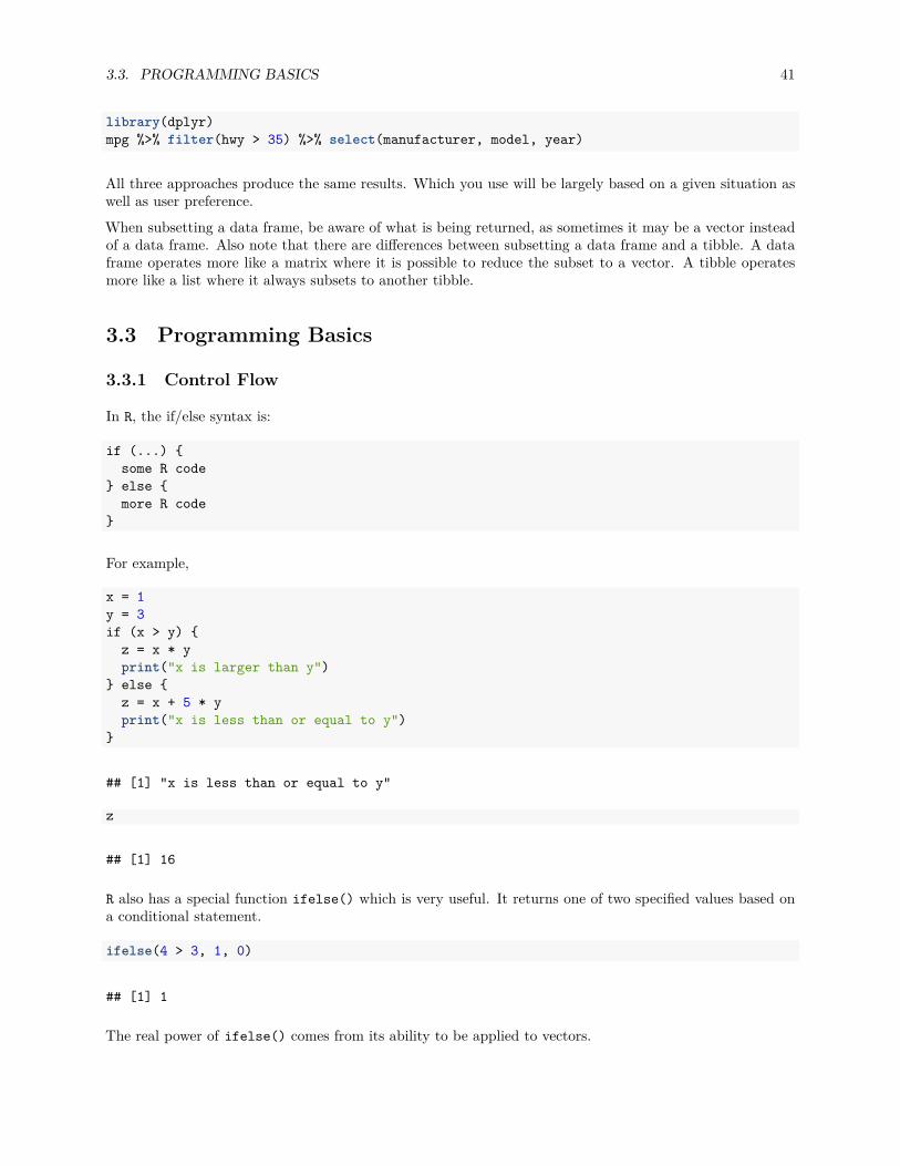
library(dplyr)mpg %>% filter(hwy > 35) %>% select(manufacturer, model, year)
All three approaches produce the same results. Which you use will be largely based on a given situation aswell as user preference.
When subsetting a data frame, be aware of what is being returned, as sometimes it may be a vector insteadof a data frame. Also note that there are differences between subsetting a data frame and a tibble. A dataframe operates more like a matrix where it is possible to reduce the subset to a vector. A tibble operatesmore like a list where it always subsets to another tibble.
3.3 Programming Basics
3.3.1 Control Flow
In R, the if/else syntax is:
if (...) {some R code
} else {more R code
}
For example,
x = 1y = 3if (x > y) {z = x * yprint("x is larger than y")
} else {z = x + 5 * yprint("x is less than or equal to y")
}
## [1] "x is less than or equal to y"
z
## [1] 16
R also has a special function ifelse() which is very useful. It returns one of two specified values based ona conditional statement.
ifelse(4 > 3, 1, 0)
## [1] 1
The real power of ifelse() comes from its ability to be applied to vectors.

42 CHAPTER 3. DATA AND PROGRAMMING
fib = c(1, 1, 2, 3, 5, 8, 13, 21)ifelse(fib > 6, "Foo", "Bar")
## [1] "Bar" "Bar" "Bar" "Bar" "Bar" "Foo" "Foo" "Foo"
Now a for loop example,
x = 11:15for (i in 1:5) {x[i] = x[i] * 2
}
x
## [1] 22 24 26 28 30
Note that this for loop is very normal in many programming languages, but not in R. In R we would not usea loop, instead we would simply use a vectorized operation.
x = 11:15x = x * 2x
## [1] 22 24 26 28 30
3.3.2 Functions
So far we have been using functions, but haven’t actually discussed some of their details.
function_name(arg1 = 10, arg2 = 20)
To use a function, you simply type its name, followed by an open parenthesis, then specify values of itsarguments, then finish with a closing parenthesis.
An argument is a variable which is used in the body of the function. Specifying the values of the argumentsis essentially providing the inputs to the function.
We can also write our own functions in R. For example, we often like to “standardize” variables, that is,subtracting the sample mean, and dividing by the sample standard deviation.
x − x
s
In R we would write a function to do this. When writing a function, there are three thing you must do.
• Give the function a name. Preferably something that is short, but descriptive.• Specify the arguments using function()• Write the body of the function within curly braces, {}.
3.3. PROGRAMMING BASICS 43
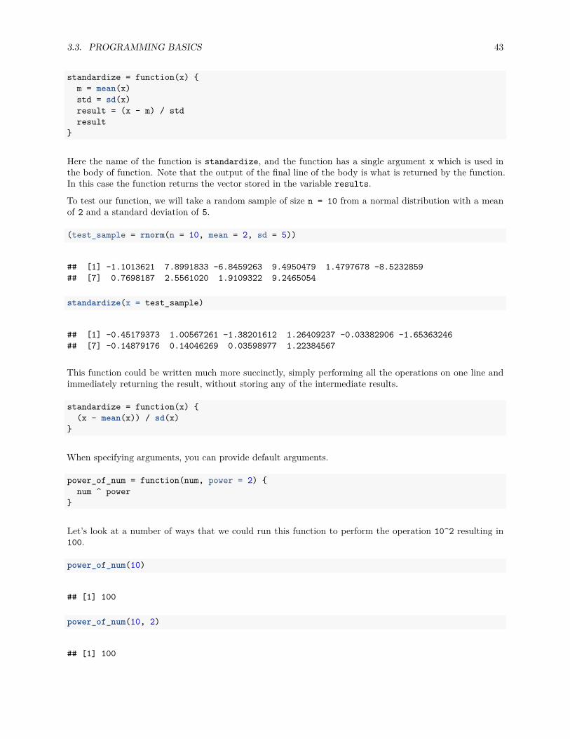
standardize = function(x) {m = mean(x)std = sd(x)result = (x - m) / stdresult
}
Here the name of the function is standardize, and the function has a single argument x which is used inthe body of function. Note that the output of the final line of the body is what is returned by the function.In this case the function returns the vector stored in the variable results.
To test our function, we will take a random sample of size n = 10 from a normal distribution with a meanof 2 and a standard deviation of 5.
(test_sample = rnorm(n = 10, mean = 2, sd = 5))
## [1] -1.1013621 7.8991833 -6.8459263 9.4950479 1.4797678 -8.5232859## [7] 0.7698187 2.5561020 1.9109322 9.2465054
standardize(x = test_sample)
## [1] -0.45179373 1.00567261 -1.38201612 1.26409237 -0.03382906 -1.65363246## [7] -0.14879176 0.14046269 0.03598977 1.22384567
This function could be written much more succinctly, simply performing all the operations on one line andimmediately returning the result, without storing any of the intermediate results.
standardize = function(x) {(x - mean(x)) / sd(x)
}
When specifying arguments, you can provide default arguments.
power_of_num = function(num, power = 2) {num ^ power
}
Let’s look at a number of ways that we could run this function to perform the operation 10^2 resulting in100.
power_of_num(10)
## [1] 100
power_of_num(10, 2)
## [1] 100
44 CHAPTER 3. DATA AND PROGRAMMING
power_of_num(num = 10, power = 2)
## [1] 100
power_of_num(power = 2, num = 10)
## [1] 100
Note that without using the argument names, the order matters. The following code will not evaluate tothe same output as the previous example.
power_of_num(2, 10)
## [1] 1024
Also, the following line of code would produce an error since arguments without a default value must bespecified.
power_of_num(power = 5)
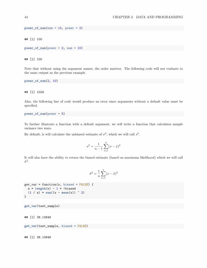
To further illustrate a function with a default argument, we will write a function that calculates samplevariance two ways.
By default, is will calculate the unbiased estimate of σ2, which we will call s2.
s2 = 1n − 1
n∑i=1
(x − x)2
It will also have the ability to return the biased estimate (based on maximum likelihood) which we will callσ2.
σ2 = 1n
n∑i=1
(x − x)2
get_var = function(x, biased = FALSE) {n = length(x) - 1 * !biased(1 / n) * sum((x - mean(x)) ^ 2)
}
get_var(test_sample)
## [1] 38.13648
get_var(test_sample, biased = FALSE)
## [1] 38.13648

3.3. PROGRAMMING BASICS 45
var(test_sample)
## [1] 38.13648
We see the function is working as expected, and when returning the unbiased estimate it matches R’s builtin function var(). Finally, let’s examine the biased estimate of σ2.
get_var(test_sample, biased = TRUE)
## [1] 34.32283

46 CHAPTER 3. DATA AND PROGRAMMING
Chapter 4
Summarizing Data
4.1 Summary Statistics
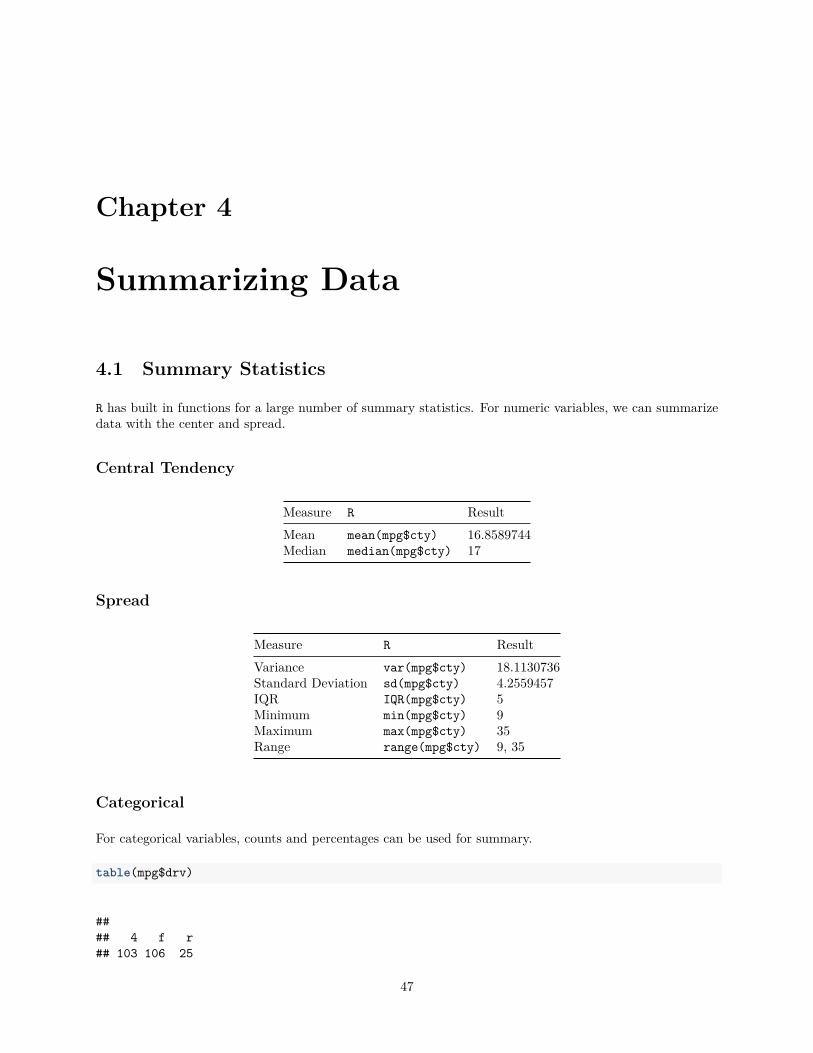
R has built in functions for a large number of summary statistics. For numeric variables, we can summarizedata with the center and spread.
Central Tendency
Measure R ResultMean mean(mpg$cty) 16.8589744Median median(mpg$cty) 17
Spread
Measure R ResultVariance var(mpg$cty) 18.1130736Standard Deviation sd(mpg$cty) 4.2559457IQR IQR(mpg$cty) 5Minimum min(mpg$cty) 9Maximum max(mpg$cty) 35Range range(mpg$cty) 9, 35
Categorical
For categorical variables, counts and percentages can be used for summary.
table(mpg$drv)
#### 4 f r## 103 106 25
47

48 CHAPTER 4. SUMMARIZING DATA
table(mpg$drv) / nrow(mpg)
#### 4 f r## 0.4401709 0.4529915 0.1068376
4.2 Plotting
Now that we have some data to work with, and we have learned about the data at the most basic level, ournext tasks is to visualize the data. Often, a proper visualization can illuminate features of the data that caninform further analysis.
We will look at four methods of visualizing data that we will use throughout the course:
• Histograms• Barplots• Boxplots• Scatterplots
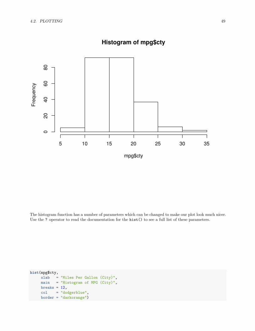
4.2.1 Histograms
When visualizing a single numerical variable, a histogram will be our go-to tool, which can be created in Rusing the hist() function.
hist(mpg$cty)
4.2. PLOTTING 49
Histogram of mpg$cty
mpg$cty
Freq
uenc
y
5 10 15 20 25 30 35
020
4060
80
The histogram function has a number of parameters which can be changed to make our plot look much nicer.Use the ? operator to read the documentation for the hist() to see a full list of these parameters.
hist(mpg$cty,xlab = "Miles Per Gallon (City)",main = "Histogram of MPG (City)",breaks = 12,col = "dodgerblue",border = "darkorange")

50 CHAPTER 4. SUMMARIZING DATA
Histogram of MPG (City)
Miles Per Gallon (City)
Freq
uenc
y
10 15 20 25 30 35
010
2030
40
Importantly, you should always be sure to label your axes and give the plot a title. The argument breaksis specific to hist(). Entering an integer will give a suggestion to R for how many bars to use for thehistogram. By default R will attempt to intelligently guess a good number of breaks, but as we can see here,it is sometimes useful to modify this yourself.
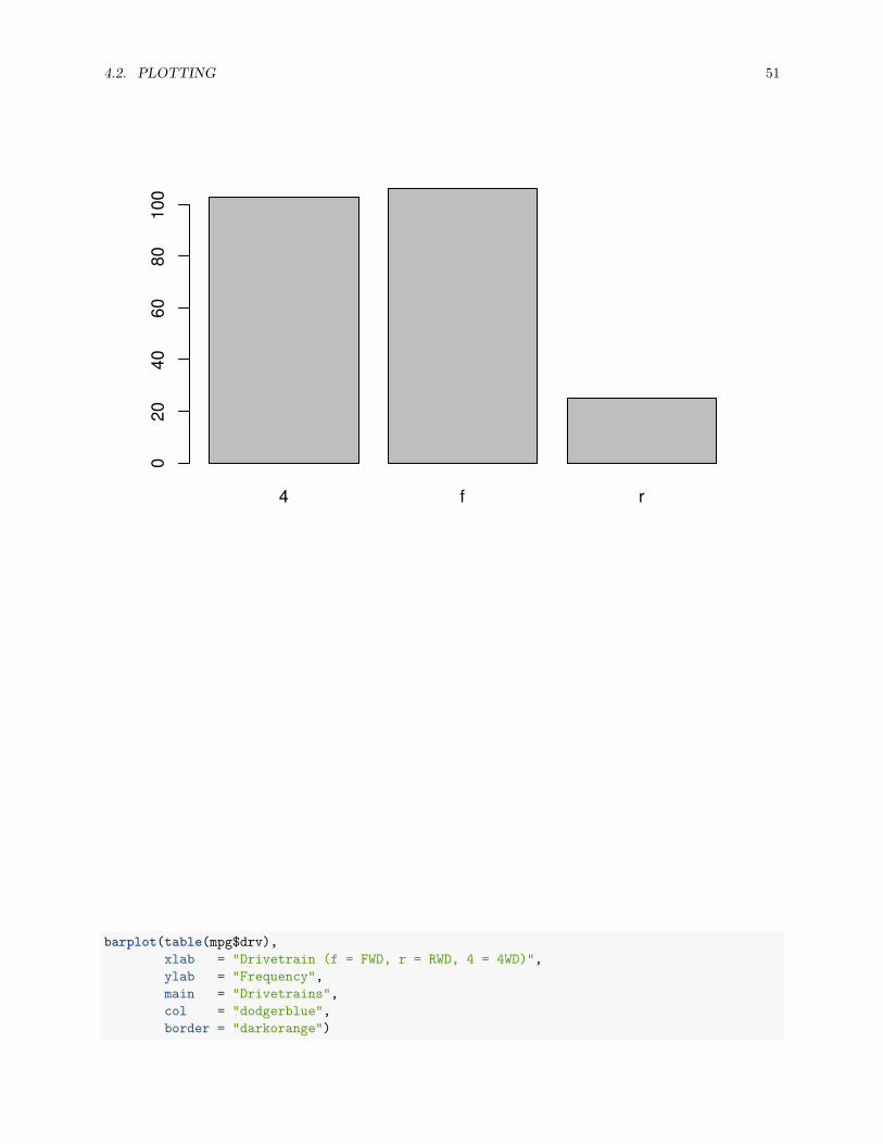
4.2.2 Barplots
Somewhat similar to a histogram, a barplot can provide a visual summary of a categorical variable, or anumeric variable with a finite number of values, like a ranking from 1 to 10.
barplot(table(mpg$drv))
4.2. PLOTTING 51
4 f r
020
4060
8010
0
barplot(table(mpg$drv),xlab = "Drivetrain (f = FWD, r = RWD, 4 = 4WD)",ylab = "Frequency",main = "Drivetrains",col = "dodgerblue",border = "darkorange")

52 CHAPTER 4. SUMMARIZING DATA
4 f r
Drivetrains
Drivetrain (f = FWD, r = RWD, 4 = 4WD)
Freq
uenc
y
020
4060
8010
0
4.2.3 Boxplots
To visualize the relationship between a numerical and categorical variable, we will use a boxplot. In thempg dataset, the drv variable takes a small, finite number of values. A car can only be front wheel drive, 4wheel drive, or rear wheel drive.
unique(mpg$drv)
## [1] "f" "4" "r"
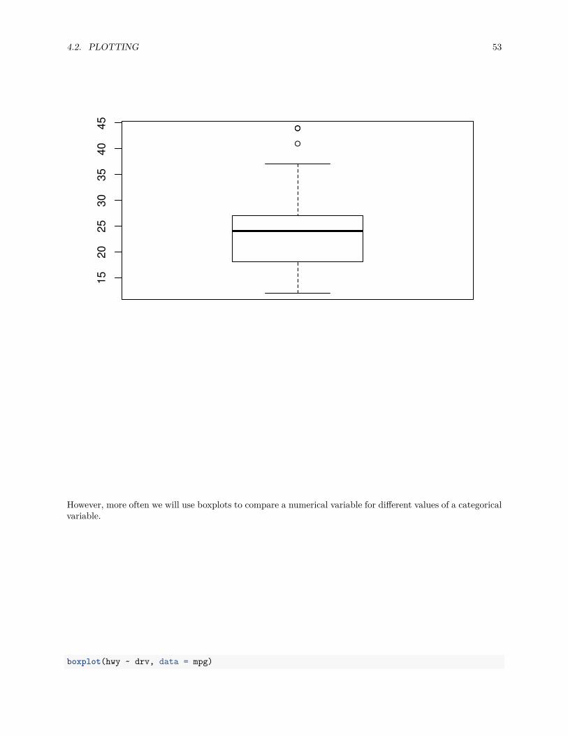
First note that we can use a single boxplot as an alternative to a histogram for visualizing a single numericalvariable. To do so in R, we use the boxplot() function.
boxplot(mpg$hwy)
4.2. PLOTTING 53
1520
2530
3540
45
However, more often we will use boxplots to compare a numerical variable for different values of a categoricalvariable.
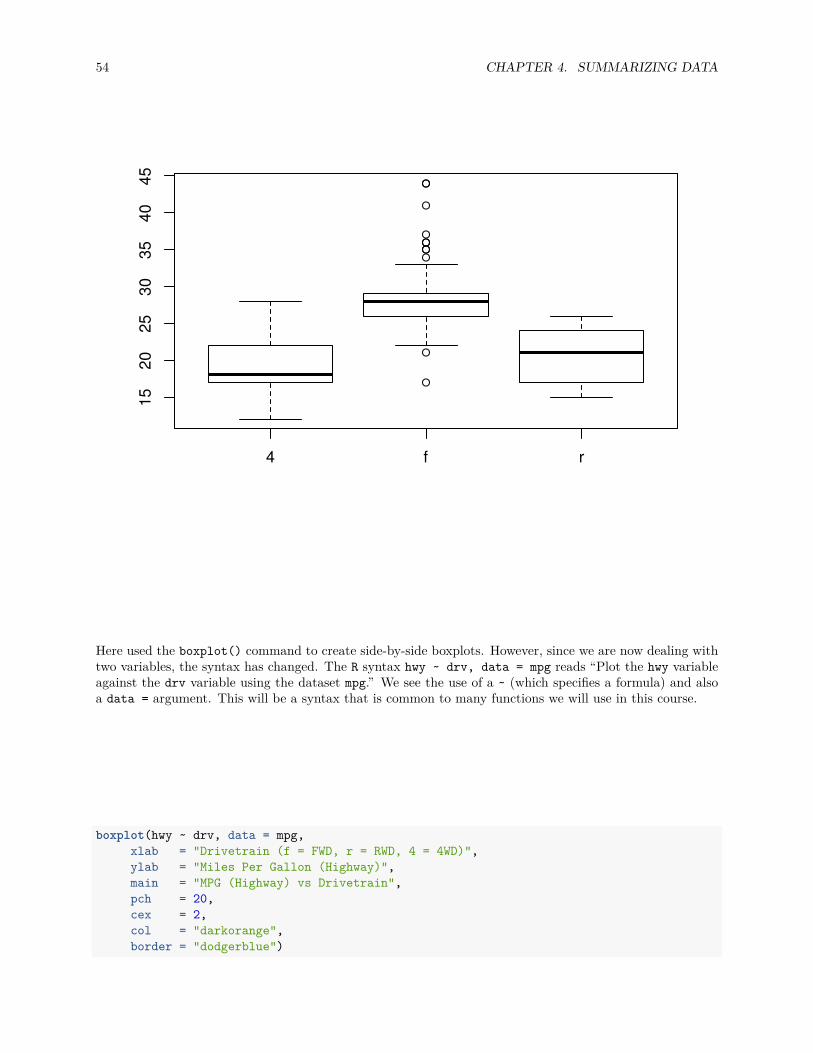
boxplot(hwy ~ drv, data = mpg)
54 CHAPTER 4. SUMMARIZING DATA
4 f r
1520
2530
3540
45
Here used the boxplot() command to create side-by-side boxplots. However, since we are now dealing withtwo variables, the syntax has changed. The R syntax hwy ~ drv, data = mpg reads “Plot the hwy variableagainst the drv variable using the dataset mpg.” We see the use of a ~ (which specifies a formula) and alsoa data = argument. This will be a syntax that is common to many functions we will use in this course.
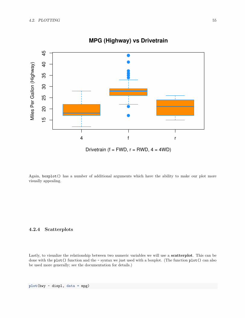
boxplot(hwy ~ drv, data = mpg,xlab = "Drivetrain (f = FWD, r = RWD, 4 = 4WD)",ylab = "Miles Per Gallon (Highway)",main = "MPG (Highway) vs Drivetrain",pch = 20,cex = 2,col = "darkorange",border = "dodgerblue")
4.2. PLOTTING 55
4 f r
1520
2530
3540
45MPG (Highway) vs Drivetrain
Drivetrain (f = FWD, r = RWD, 4 = 4WD)
Mile
s P
er G
allo
n (H
ighw
ay)
Again, boxplot() has a number of additional arguments which have the ability to make our plot morevisually appealing.
4.2.4 Scatterplots
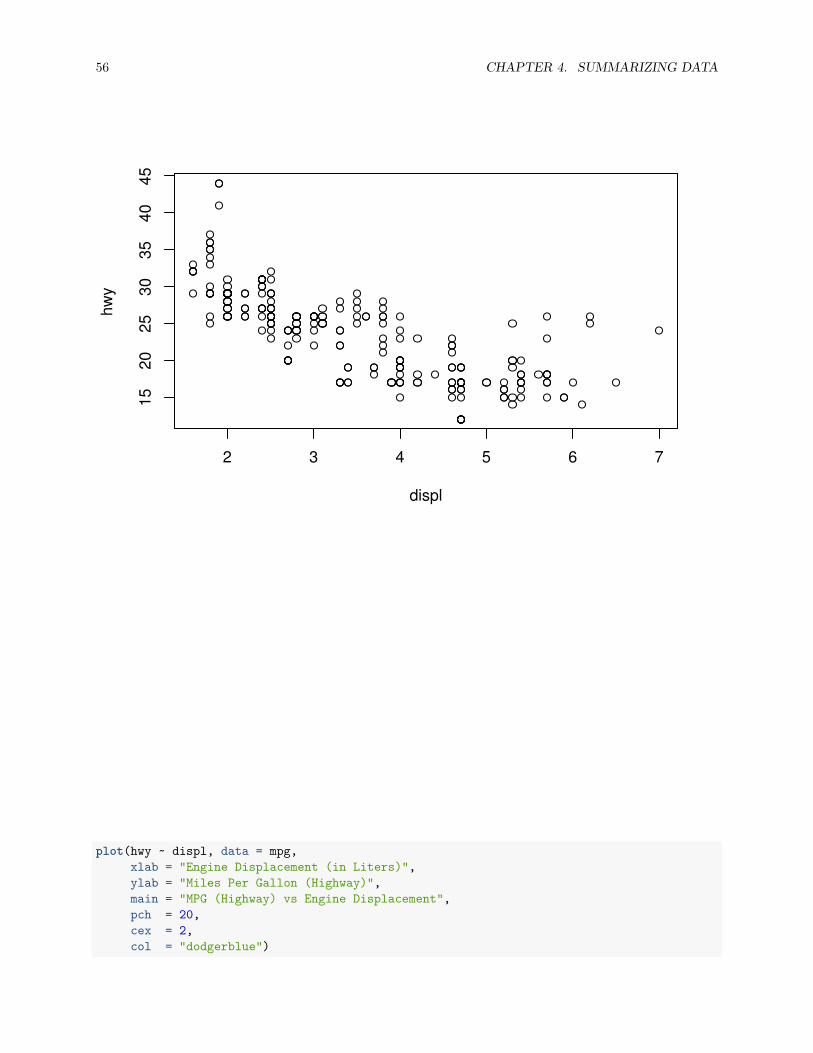
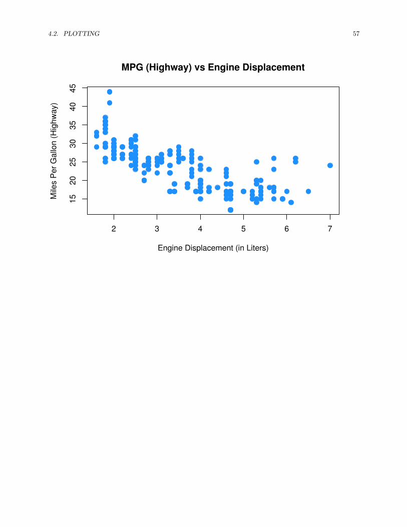
Lastly, to visualize the relationship between two numeric variables we will use a scatterplot. This can bedone with the plot() function and the ~ syntax we just used with a boxplot. (The function plot() can alsobe used more generally; see the documentation for details.)
plot(hwy ~ displ, data = mpg)
56 CHAPTER 4. SUMMARIZING DATA
2 3 4 5 6 7
1520
2530
3540
45
displ
hwy
plot(hwy ~ displ, data = mpg,xlab = "Engine Displacement (in Liters)",ylab = "Miles Per Gallon (Highway)",main = "MPG (Highway) vs Engine Displacement",pch = 20,cex = 2,col = "dodgerblue")
4.2. PLOTTING 57
2 3 4 5 6 7
1520
2530
3540
45MPG (Highway) vs Engine Displacement
Engine Displacement (in Liters)
Mile
s P
er G
allo
n (H
ighw
ay)

58 CHAPTER 4. SUMMARIZING DATA

Chapter 5
Probability and Statistics in R
5.1 Probability in R
5.1.1 Distributions
When working with different statistical distributions, we often want to make probabilistic statements basedon the distribution.We typically want to know one of four things:
• The density (pdf) at a particular value.• The distribution (cdf) at a particular value.• The quantile value corresponding to a particular probability.• A random draw of values from a particular distribution.
This used to be done with statistical tables printed in the back of textbooks. Now, R has functions forobtaining density, distribution, quantile and random values.The general naming structure of the relevant R functions is:
• dname calculates density (pdf) at input x.• pname calculates distribution (cdf) at input x.• qname calculates the quantile at an input probability.• rname generates a random draw from a particular distribution.
Note that name represents the name of the given distribution.For example, consider a random variable X which is N(µ = 2, σ2 = 25). (Note, we are parameterizing usingthe variance σ2. R however uses the standard deviation.)To calculate the value of the pdf at x = 3, that is, the height of the curve at x = 3, use:
dnorm(x = 3, mean = 2, sd = 5)
## [1] 0.07820854
To calculate the value of the cdf at x = 3, that is, P (X ≤ 3), the probability that X is less than or equal to3, use:
59
60 CHAPTER 5. PROBABILITY AND STATISTICS IN R
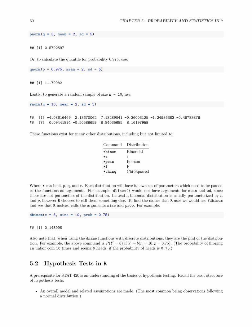
pnorm(q = 3, mean = 2, sd = 5)
## [1] 0.5792597
Or, to calculate the quantile for probability 0.975, use:
qnorm(p = 0.975, mean = 2, sd = 5)
## [1] 11.79982
Lastly, to generate a random sample of size n = 10, use:
rnorm(n = 10, mean = 2, sd = 5)
## [1] -4.08616469 2.13670062 7.13289041 -0.36003125 -1.24936383 -0.48783376## [7] 0.09441894 -0.50586659 8.84035685 8.16197959
These functions exist for many other distributions, including but not limited to:
Command Distribution*binom Binomial*t t*pois Poisson*f F*chisq Chi-Squared
Where * can be d, p, q, and r. Each distribution will have its own set of parameters which need to be passedto the functions as arguments. For example, dbinom() would not have arguments for mean and sd, sincethose are not parameters of the distribution. Instead a binomial distribution is usually parameterized by nand p, however R chooses to call them something else. To find the names that R uses we would use ?dbinomand see that R instead calls the arguments size and prob. For example:
dbinom(x = 6, size = 10, prob = 0.75)
## [1] 0.145998
Also note that, when using the dname functions with discrete distributions, they are the pmf of the distribu-tion. For example, the above command is P (Y = 6) if Y ∼ b(n = 10, p = 0.75). (The probability of flippingan unfair coin 10 times and seeing 6 heads, if the probability of heads is 0.75.)
5.2 Hypothesis Tests in R
A prerequisite for STAT 420 is an understanding of the basics of hypothesis testing. Recall the basic structureof hypothesis tests:
• An overall model and related assumptions are made. (The most common being observations followinga normal distribution.)
5.2. HYPOTHESIS TESTS IN R 61
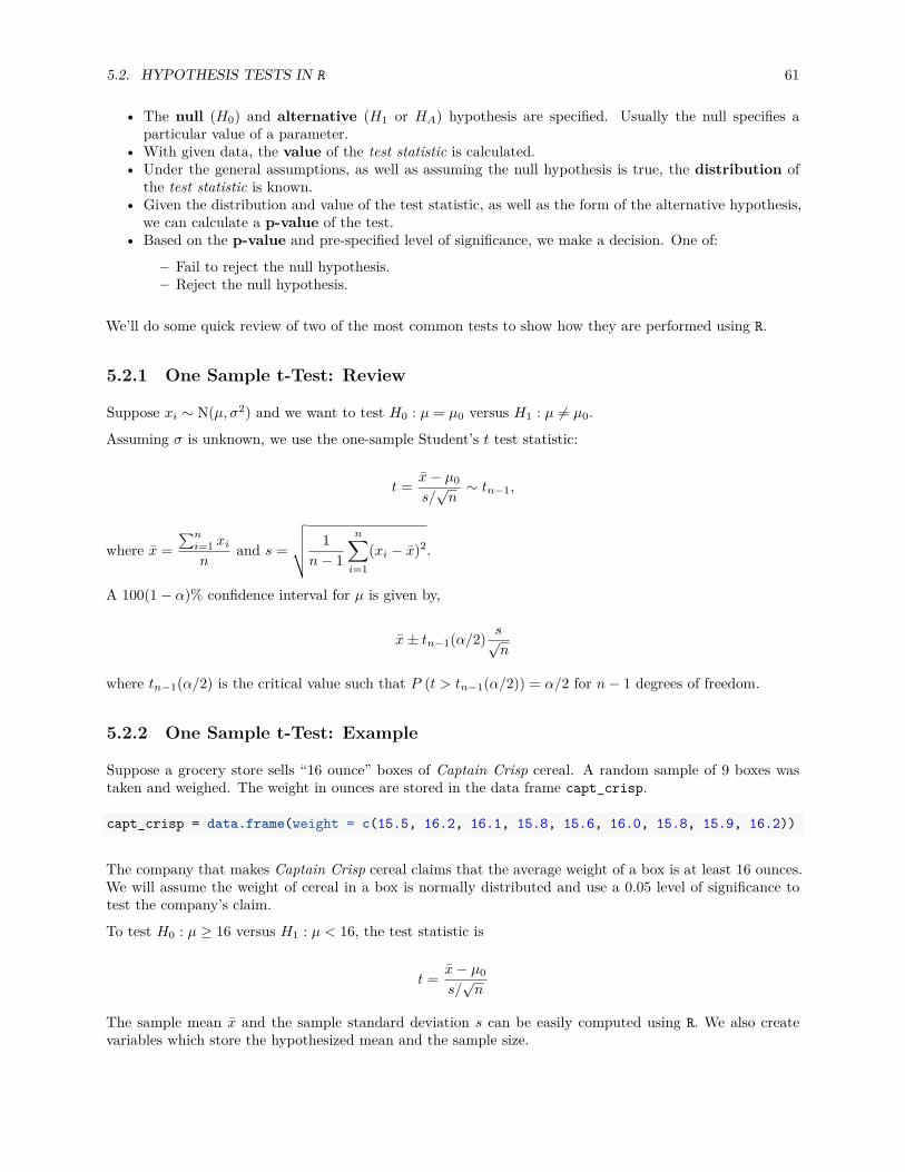
• The null (H0) and alternative (H1 or HA) hypothesis are specified. Usually the null specifies aparticular value of a parameter.
• With given data, the value of the test statistic is calculated.• Under the general assumptions, as well as assuming the null hypothesis is true, the distribution of
the test statistic is known.• Given the distribution and value of the test statistic, as well as the form of the alternative hypothesis,
we can calculate a p-value of the test.• Based on the p-value and pre-specified level of significance, we make a decision. One of:
– Fail to reject the null hypothesis.– Reject the null hypothesis.
We’ll do some quick review of two of the most common tests to show how they are performed using R.
5.2.1 One Sample t-Test: Review
Suppose xi ∼ N(µ, σ2) and we want to test H0 : µ = µ0 versus H1 : µ = µ0.
Assuming σ is unknown, we use the one-sample Student’s t test statistic:
t = x − µ0
s/√
n∼ tn−1,
where x =∑n
i=1 xi
nand s =
√√√√ 1n − 1
n∑i=1
(xi − x)2.
A 100(1 − α)% confidence interval for µ is given by,
x ± tn−1(α/2) s√n
where tn−1(α/2) is the critical value such that P (t > tn−1(α/2)) = α/2 for n − 1 degrees of freedom.
5.2.2 One Sample t-Test: Example
Suppose a grocery store sells “16 ounce” boxes of Captain Crisp cereal. A random sample of 9 boxes wastaken and weighed. The weight in ounces are stored in the data frame capt_crisp.
capt_crisp = data.frame(weight = c(15.5, 16.2, 16.1, 15.8, 15.6, 16.0, 15.8, 15.9, 16.2))
The company that makes Captain Crisp cereal claims that the average weight of a box is at least 16 ounces.We will assume the weight of cereal in a box is normally distributed and use a 0.05 level of significance totest the company’s claim.
To test H0 : µ ≥ 16 versus H1 : µ < 16, the test statistic is
t = x − µ0
s/√
n
The sample mean x and the sample standard deviation s can be easily computed using R. We also createvariables which store the hypothesized mean and the sample size.

62 CHAPTER 5. PROBABILITY AND STATISTICS IN R
x_bar = mean(capt_crisp$weight)s = sd(capt_crisp$weight)mu_0 = 16n = 9
We can then easily compute the test statistic.
t = (x_bar - mu_0) / (s / sqrt(n))t
## [1] -1.2
Under the null hypothesis, the test statistic has a t distribution with n − 1 degrees of freedom, in this case 8.
To complete the test, we need to obtain the p-value of the test. Since this is a one-sided test with a less-thanalternative, we need to area to the left of -1.2 for a t distribution with 8 degrees of freedom. That is,
P (t8 < −1.2)
pt(t, df = n - 1)
## [1] 0.1322336
We now have the p-value of our test, which is greater than our significance level (0.05), so we fail to rejectthe null hypothesis.
Alternatively, this entire process could have been completed using one line of R code.
t.test(x = capt_crisp$weight, mu = 16, alternative = c("less"), conf.level = 0.95)
#### One Sample t-test#### data: capt_crisp$weight## t = -1.2, df = 8, p-value = 0.1322## alternative hypothesis: true mean is less than 16## 95 percent confidence interval:## -Inf 16.05496## sample estimates:## mean of x## 15.9
We supply R with the data, the hypothesized value of µ, the alternative, and the confidence level. R thenreturns a wealth of information including:
• The value of the test statistic.• The degrees of freedom of the distribution under the null hypothesis.• The p-value of the test.• The confidence interval which corresponds to the test.• An estimate of µ.

5.2. HYPOTHESIS TESTS IN R 63
Since the test was one-sided, R returned a one-sided confidence interval. If instead we wanted a two-sidedinterval for the mean weight of boxes of Captain Crisp cereal we could modify our code.
capt_test_results = t.test(capt_crisp$weight, mu = 16,alternative = c("two.sided"), conf.level = 0.95)
This time we have stored the results. By doing so, we can directly access portions of the output fromt.test(). To see what information is available we use the names() function.
names(capt_test_results)
## [1] "statistic" "parameter" "p.value" "conf.int" "estimate"## [6] "null.value" "alternative" "method" "data.name"
We are interested in the confidence interval which is stored in conf.int.
capt_test_results$conf.int
## [1] 15.70783 16.09217## attr(,"conf.level")## [1] 0.95
Let’s check this interval “by hand.” The one piece of information we are missing is the critical value,tn−1(α/2) = t8(0.025), which can be calculated in R using the qt() function.
qt(0.975, df = 8)
## [1] 2.306004
So, the 95% CI for the mean weight of a cereal box is calculated by plugging into the formula,
x ± tn−1(α/2) s√n
c(mean(capt_crisp$weight) - qt(0.975, df = 8) * sd(capt_crisp$weight) / sqrt(9),mean(capt_crisp$weight) + qt(0.975, df = 8) * sd(capt_crisp$weight) / sqrt(9))
## [1] 15.70783 16.09217
5.2.3 Two Sample t-Test: Review
Suppose xi ∼ N(µx, σ2) and yi ∼ N(µy, σ2).
Want to test H0 : µx − µy = µ0 versus H1 : µx − µy = µ0.
Assuming σ is unknown, use the two-sample Student’s t test statistic:
t = (x − y) − µ0
sp
√1n + 1
m
∼ tn+m−2,
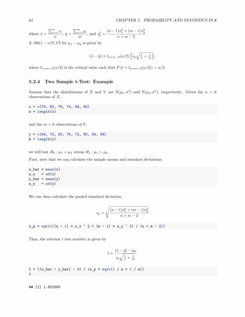
64 CHAPTER 5. PROBABILITY AND STATISTICS IN R
where x =∑n
i=1 xi
n, y =
∑mi=1 yi
m, and s2
p =(n − 1)s2
x + (m − 1)s2y
n + m − 2.
A 100(1 − α)% CI for µx − µy is given by
(x − y) ± tn+m−2(α/2)(
sp
√1n + 1
m
),
where tn+m−2(α/2) is the critical value such that P (t > tn+m−2(α/2)) = α/2.
5.2.4 Two Sample t-Test: Example
Assume that the distributions of X and Y are N(µ1, σ2) and N(µ2, σ2), respectively. Given the n = 6observations of X,
x = c(70, 82, 78, 74, 94, 82)n = length(x)
and the m = 8 observations of Y ,
y = c(64, 72, 60, 76, 72, 80, 84, 68)m = length(y)
we will test H0 : µ1 = µ2 versus H1 : µ1 > µ2.
First, note that we can calculate the sample means and standard deviations.
x_bar = mean(x)s_x = sd(x)y_bar = mean(y)s_y = sd(y)
We can then calculate the pooled standard deviation.
sp =
√(n − 1)s2
x + (m − 1)s2y
n + m − 2
s_p = sqrt(((n - 1) * s_x ^ 2 + (m - 1) * s_y ^ 2) / (n + m - 2))
Thus, the relevant t test statistic is given by
t = (x − y) − µ0
sp
√1n + 1
m
.
t = ((x_bar - y_bar) - 0) / (s_p * sqrt(1 / n + 1 / m))t
## [1] 1.823369

5.2. HYPOTHESIS TESTS IN R 65
Note that t ∼ tn+m−2 = t12, so we can calculate the p-value, which is
P (t12 > 1.8233692).
1 - pt(t, df = n + m - 2)
## [1] 0.04661961
But, then again, we could have simply performed this test in one line of R.
t.test(x, y, alternative = c("greater"), var.equal = TRUE)
#### Two Sample t-test#### data: x and y## t = 1.8234, df = 12, p-value = 0.04662## alternative hypothesis: true difference in means is greater than 0## 95 percent confidence interval:## 0.1802451 Inf## sample estimates:## mean of x mean of y## 80 72
Recall that a two-sample t-test can be done with or without an equal variance assumption. Here var.equal= TRUE tells R we would like to perform the test under the equal variance assumption.Above we carried out the analysis using two vectors x and y. In general, we will have a preference for usingdata frames.
t_test_data = data.frame(values = c(x, y),group = c(rep("A", length(x)), rep("B", length(y))))
We now have the data stored in a single variables (values) and have created a second variable (group) whichindicates which “sample” the value belongs to.
t_test_data
## values group## 1 70 A## 2 82 A## 3 78 A## 4 74 A## 5 94 A## 6 82 A## 7 64 B## 8 72 B## 9 60 B## 10 76 B## 11 72 B## 12 80 B## 13 84 B## 14 68 B
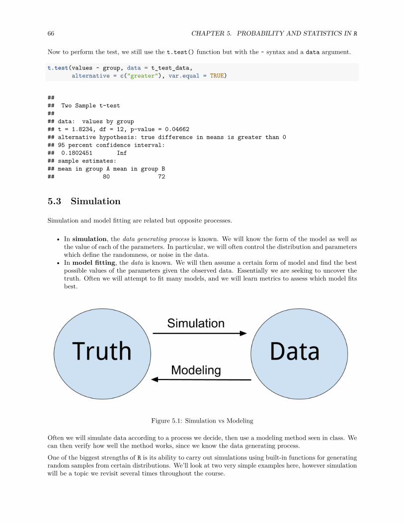
66 CHAPTER 5. PROBABILITY AND STATISTICS IN R
Now to perform the test, we still use the t.test() function but with the ~ syntax and a data argument.
t.test(values ~ group, data = t_test_data,alternative = c("greater"), var.equal = TRUE)
#### Two Sample t-test#### data: values by group## t = 1.8234, df = 12, p-value = 0.04662## alternative hypothesis: true difference in means is greater than 0## 95 percent confidence interval:## 0.1802451 Inf## sample estimates:## mean in group A mean in group B## 80 72
5.3 Simulation
Simulation and model fitting are related but opposite processes.
• In simulation, the data generating process is known. We will know the form of the model as well asthe value of each of the parameters. In particular, we will often control the distribution and parameterswhich define the randomness, or noise in the data.
• In model fitting, the data is known. We will then assume a certain form of model and find the bestpossible values of the parameters given the observed data. Essentially we are seeking to uncover thetruth. Often we will attempt to fit many models, and we will learn metrics to assess which model fitsbest.
Figure 5.1: Simulation vs Modeling
Often we will simulate data according to a process we decide, then use a modeling method seen in class. Wecan then verify how well the method works, since we know the data generating process.
One of the biggest strengths of R is its ability to carry out simulations using built-in functions for generatingrandom samples from certain distributions. We’ll look at two very simple examples here, however simulationwill be a topic we revisit several times throughout the course.

5.3. SIMULATION 67
5.3.1 Paired Differences
Consider the model:
X11, X12, . . . , X1n ∼ N(µ1, σ2)X21, X22, . . . , X2n ∼ N(µ2, σ2)
Assume that µ1 = 6, µ2 = 5, σ2 = 4 and n = 25.
Let
X1 = 1n
n∑i=1
X1i
X2 = 1n
n∑i=1
X2i
D = X1 − X2.
Suppose we would like to calculate P (0 < D < 2). First we will need to obtain the distribution of D.
Recall,
X1 ∼ N
(µ1,
σ2
n
)and
X2 ∼ N
(µ2,
σ2
n
).
Then,
D = X1 − X2 ∼ N
(µ1 − µ2,
σ2
n+ σ2
n
)= N
(6 − 5,
425
+ 425
).
So,
D ∼ N(µ = 1, σ2 = 0.32).
Thus,
P (0 < D < 2) = P (D < 2) − P (D < 0).
This can then be calculated using R without a need to first standardize, or use a table.
pnorm(2, mean = 1, sd = sqrt(0.32)) - pnorm(0, mean = 1, sd = sqrt(0.32))
## [1] 0.9229001

68 CHAPTER 5. PROBABILITY AND STATISTICS IN R
An alternative approach, would be to simulate a large number of observations of D then use the empiricaldistribution to calculate the probability.
Our strategy will be to repeatedly:
• Generate a sample of 25 random observations from N(µ1 = 6, σ2 = 4). Call the mean of this samplex1s.
• Generate a sample of 25 random observations from N(µ1 = 5, σ2 = 4). Call the mean of this samplex2s.
• Calculate the differences of the means, ds = x1s − x2s.
We will repeat the process a large number of times. Then we will use the distribution of the simulatedobservations of ds as an estimate for the true distribution of D.
set.seed(42)num_samples = 10000differences = rep(0, num_samples)
Before starting our for loop to perform the operation, we set a seed for reproducibility, create and set avariable num_samples which will define the number of repetitions, and lastly create a variables differenceswhich will store the simulate values, ds.
By using set.seed() we can reproduce the random results of rnorm() each time starting from that line.
for (s in 1:num_samples) {x1 = rnorm(n = 25, mean = 6, sd = 2)x2 = rnorm(n = 25, mean = 5, sd = 2)differences[s] = mean(x1) - mean(x2)
}
To estimate P (0 < D < 2) we will find the proportion of values of ds (among the 10000 values of ds generated)that are between 0 and 2.
mean(0 < differences & differences < 2)
## [1] 0.9222
Recall that above we derived the distribution of D to be N(µ = 1, σ2 = 0.32)
If we look at a histogram of the differences, we find that it looks very much like a normal distribution.
hist(differences, breaks = 20,main = "Empirical Distribution of D",xlab = "Simulated Values of D",col = "dodgerblue",border = "darkorange")

5.3. SIMULATION 69
Empirical Distribution of D
Simulated Values of D
Freq
uenc
y
-1 0 1 2 3
020
060
010
0014
00
Also the sample mean and variance are very close to to what we would expect.
mean(differences)
## [1] 1.001423
var(differences)
## [1] 0.3230183
We could have also accomplished this task with a single line of more “idiomatic” R.
set.seed(42)diffs = replicate(10000, mean(rnorm(25, 6, 2)) - mean(rnorm(25, 5, 2)))
Use ?replicate to take a look at the documentation for the replicate function and see if you can under-stand how this line performs the same operations that our for loop above executed.
mean(differences == diffs)
## [1] 1
We see that by setting the same seed for the randomization, we actually obtain identical results!

70 CHAPTER 5. PROBABILITY AND STATISTICS IN R
5.3.2 Distribution of a Sample Mean
For another example of simulation, we will simulate observations from a Poisson distribution, and examinethe empirical distribution of the sample mean of these observations.
Recall, if
X ∼ Pois(µ)
then
E[X] = µ
and
V ar[X] = µ.
Also, recall that for a random variable X with finite mean µ and finite variance σ2, the central limit theoremtells us that the mean, X of a random sample of size n is approximately normal for large values of n.Specifically, as n → ∞,
Xd→ N
(µ,
σ2
n
).
The following verifies this result for a Poisson distribution with µ = 10 and a sample size of n = 50.
set.seed(1337)mu = 10sample_size = 50samples = 100000x_bars = rep(0, samples)
for(i in 1:samples){x_bars[i] = mean(rpois(sample_size, lambda = mu))
}
x_bar_hist = hist(x_bars, breaks = 50,main = "Histogram of Sample Means",xlab = "Sample Means")

5.3. SIMULATION 71
Histogram of Sample Means
Sample Means
Freq
uenc
y
8 9 10 11 12
020
0040
0060
0080
00
Now we will compare sample statistics from the empirical distribution with their known values based on theparent distribution.
c(mean(x_bars), mu)
## [1] 10.00008 10.00000
c(var(x_bars), mu / sample_size)
## [1] 0.1989732 0.2000000
c(sd(x_bars), sqrt(mu) / sqrt(sample_size))
## [1] 0.4460641 0.4472136
And here, we will calculate the proportion of sample means that are within 2 standard deviations of thepopulation mean.
mean(x_bars > mu - 2 * sqrt(mu) / sqrt(sample_size) &x_bars < mu + 2 * sqrt(mu) / sqrt(sample_size))
## [1] 0.95429

72 CHAPTER 5. PROBABILITY AND STATISTICS IN R
This last histogram uses a bit of a trick to approximately shade the bars that are within two standarddeviations of the mean.)
shading = ifelse(x_bar_hist$breaks > mu - 2 * sqrt(mu) / sqrt(sample_size) &x_bar_hist$breaks < mu + 2 * sqrt(mu) / sqrt(sample_size),"darkorange", "dodgerblue")
x_bar_hist = hist(x_bars, breaks = 50, col = shading,main = "Histogram of Sample Means, Two Standard Deviations",xlab = "Sample Means")
Histogram of Sample Means, Two Standard Deviations
Sample Means
Freq
uenc
y
8 9 10 11 12
020
0040
0060
0080
00

Chapter 6
R Resources
So far, we have seen a lot of R, and a lot of R quickly. Again, the preceding chapters were in no way meantto be a complete reference for the R language, but rather an introduction to many of the concepts we willneed in this text. The following resources are not necessary for the remainder of this text, but you may findthem useful if you would like a deeper understanding of R:
6.1 Beginner Tutorials and References
• Try R from Code School.
– An interactive introduction to the basics of R. Useful for getting up to speed on R’s syntax.
• Quick-R by Robert Kabacoff.
– A good reference for R basics.
• R Tutorial by Chi Yau.
– A combination reference and tutorial for R basics.
• R Programming for Data Science by Roger Peng
– A great text for R programming beginners. Discusses R from the ground up, highlighting program-ming details we might not discuss.
6.2 Intermediate References
• R for Data Science by Hadley Wickham and Garrett Grolemund.
– Similar to Advanced R, but focuses more on data analysis, while still introducing programmingconcepts. Especially useful for working in the tidyverse.
• The Art of R Programming by Norman Matloff.
– Gentle introduction to the programming side of R. (Whereas we will focus more on the dataanalysis side.) A free electronic version is available through the Illinois library.
73

74 CHAPTER 6. R RESOURCES
6.3 Advanced References
• Advanced R by Hadley Wickham.
– From the author of several extremely popular R packages. Good follow-up to The Art of RProgramming. (And more up-to-date material.)
• The R Inferno by Patrick Burns.
– Likens learning the tricks of R to descending through the levels of hell. Very advanced material,but may be important if R becomes a part of your everyday toolkit.
• Efficient R Programming by Colin Gillespie and Robin Lovelace
– Discusses both efficient R programs, as well as programming in R efficiently.
6.4 Quick Comparisons to Other Languages
Those who are familiar with other languages may find the following “cheatsheets” helpful for transitioningto R.
• MATLAB, NumPy, Julia• Stata• SAS - Look for a resource still! Suggestions welcome.
6.5 RStudio and RMarkdown Videos
The following video playlists were made as an introduction to R, RStudio, and RMarkdown for STAT 420 atUIUC. If you are currently using this text for a Coursera course, you can also find updated videos there.
• R and RStudio• Data in R• RMarkdown
Note that RStudio and RMarkdown are constantly receiving excellent support and updates, so these videosmay already contain some outdated information.
RStudio provides their own tutorial for RMarkdown. They also have an excellent RStudio “cheatsheets”which visually identifies many of the features available in the IDE.
6.6 RMarkdown Template
This .zip file contains the files necessary to produce this rendered document. This document is a morecomplete version of a template than what is seen in the above videos.
Chapter 7
Simple Linear Regression
“All models are wrong, but some are useful.”— George E. P. Box
After reading this chapter you will be able to:
• Understand the concept of a model.• Describe two ways in which regression coefficients are derived.• Estimate and visualize a regression model using R.• Interpret regression coefficients and statistics in the context of real-world problems.• Use a regression model to make predictions.
7.1 Modeling
Let’s consider a simple example of how the speed of a car affects its stopping distance, that is, how far ittravels before it comes to a stop. To examine this relationship, we will use the cars dataset which, is adefault R dataset. Thus, we don’t need to load a package first; it is immediately available.
To get a first look at the data you can use the View() function inside RStudio.
View(cars)
We could also take a look at the variable names, the dimension of the data frame, and some sample obser-vations with str().
str(cars)
## 'data.frame': 50 obs. of 2 variables:## $ speed: num 4 4 7 7 8 9 10 10 10 11 ...## $ dist : num 2 10 4 22 16 10 18 26 34 17 ...
As we have seen before with data frames, there are a number of additional functions to access some of thisinformation directly.
75

76 CHAPTER 7. SIMPLE LINEAR REGRESSION
dim(cars)
## [1] 50 2
nrow(cars)
## [1] 50
ncol(cars)
## [1] 2
Other than the two variable names and the number of observations, this data is still just a bunch of numbers,so we should probably obtain some context.
?cars
Reading the documentation we learn that this is data gathered during the 1920s about the speed of carsand the resulting distance it takes for the car to come to a stop. The interesting task here is to determinehow far a car travels before stopping, when traveling at a certain speed. So, we will first plot the stoppingdistance against the speed.
plot(dist ~ speed, data = cars,xlab = "Speed (in Miles Per Hour)",ylab = "Stopping Distance (in Feet)",main = "Stopping Distance vs Speed",pch = 20,cex = 2,col = "grey")
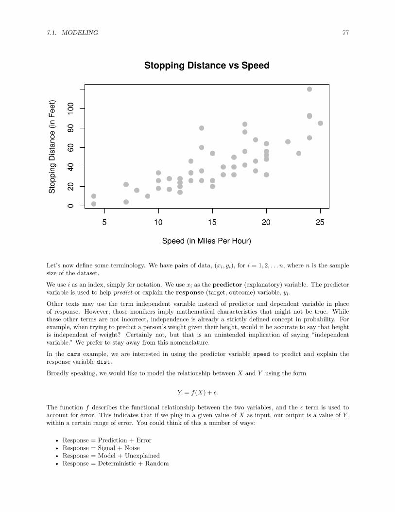
7.1. MODELING 77
5 10 15 20 25
020
4060
8010
0Stopping Distance vs Speed
Speed (in Miles Per Hour)
Sto
ppin
g D
ista
nce
(in F
eet)
Let’s now define some terminology. We have pairs of data, (xi, yi), for i = 1, 2, . . . n, where n is the samplesize of the dataset.
We use i as an index, simply for notation. We use xi as the predictor (explanatory) variable. The predictorvariable is used to help predict or explain the response (target, outcome) variable, yi.
Other texts may use the term independent variable instead of predictor and dependent variable in placeof response. However, those monikers imply mathematical characteristics that might not be true. Whilethese other terms are not incorrect, independence is already a strictly defined concept in probability. Forexample, when trying to predict a person’s weight given their height, would it be accurate to say that heightis independent of weight? Certainly not, but that is an unintended implication of saying “independentvariable.” We prefer to stay away from this nomenclature.
In the cars example, we are interested in using the predictor variable speed to predict and explain theresponse variable dist.
Broadly speaking, we would like to model the relationship between X and Y using the form
Y = f(X) + ϵ.
The function f describes the functional relationship between the two variables, and the ϵ term is used toaccount for error. This indicates that if we plug in a given value of X as input, our output is a value of Y ,within a certain range of error. You could think of this a number of ways:
• Response = Prediction + Error• Response = Signal + Noise• Response = Model + Unexplained• Response = Deterministic + Random
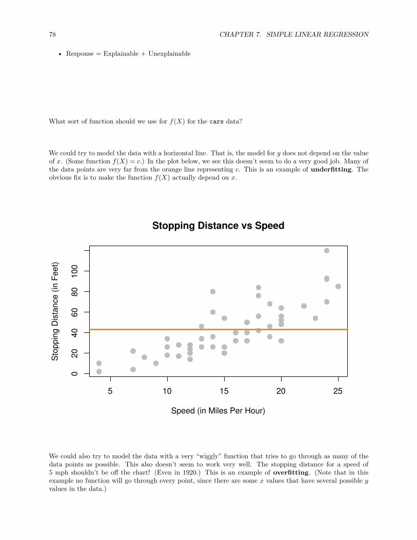
78 CHAPTER 7. SIMPLE LINEAR REGRESSION
• Response = Explainable + Unexplainable
What sort of function should we use for f(X) for the cars data?
We could try to model the data with a horizontal line. That is, the model for y does not depend on the valueof x. (Some function f(X) = c.) In the plot below, we see this doesn’t seem to do a very good job. Many ofthe data points are very far from the orange line representing c. This is an example of underfitting. Theobvious fix is to make the function f(X) actually depend on x.
5 10 15 20 25
020
4060
8010
0
Stopping Distance vs Speed
Speed (in Miles Per Hour)
Sto
ppin
g D
ista
nce
(in F
eet)
We could also try to model the data with a very “wiggly” function that tries to go through as many of thedata points as possible. This also doesn’t seem to work very well. The stopping distance for a speed of5 mph shouldn’t be off the chart! (Even in 1920.) This is an example of overfitting. (Note that in thisexample no function will go through every point, since there are some x values that have several possible yvalues in the data.)
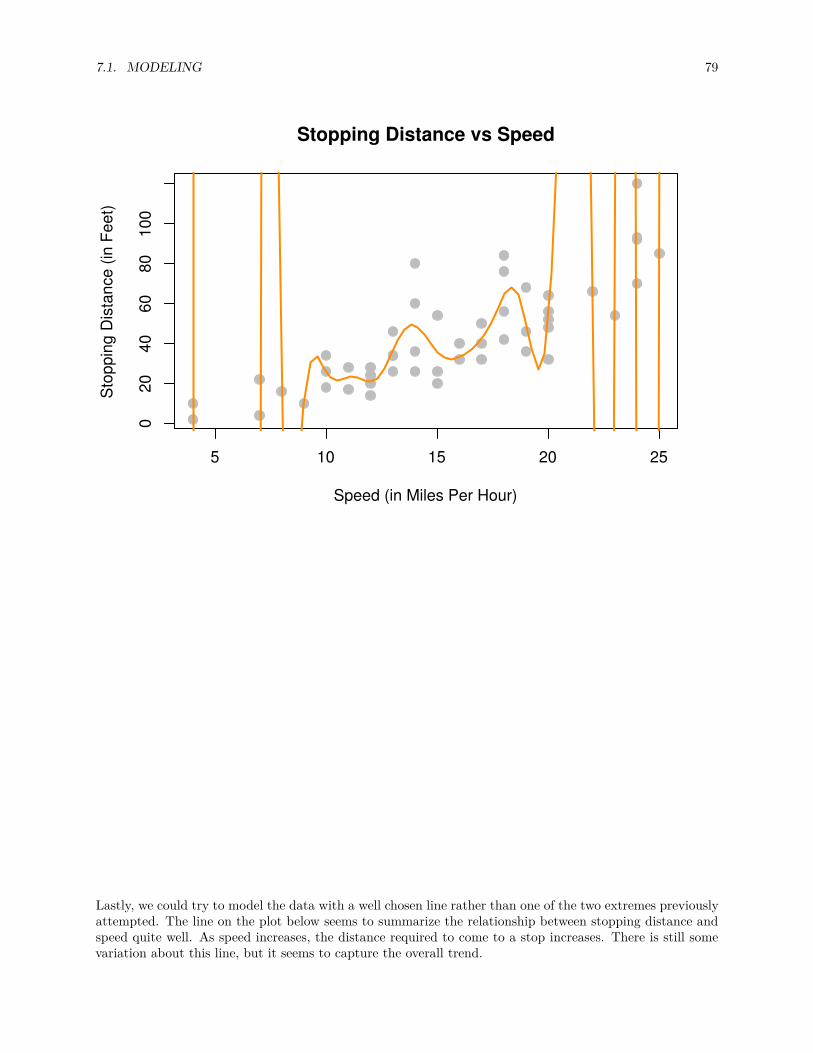
7.1. MODELING 79
5 10 15 20 25
020
4060
8010
0Stopping Distance vs Speed
Speed (in Miles Per Hour)
Sto
ppin
g D
ista
nce
(in F
eet)
Lastly, we could try to model the data with a well chosen line rather than one of the two extremes previouslyattempted. The line on the plot below seems to summarize the relationship between stopping distance andspeed quite well. As speed increases, the distance required to come to a stop increases. There is still somevariation about this line, but it seems to capture the overall trend.
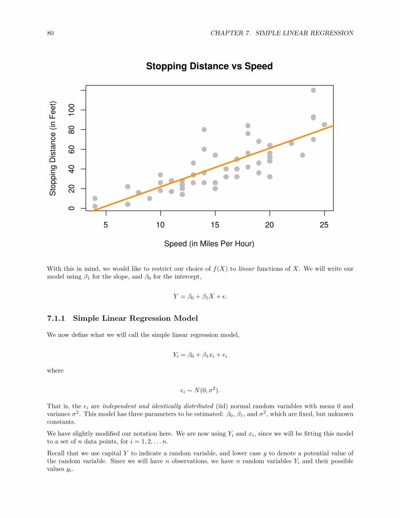
80 CHAPTER 7. SIMPLE LINEAR REGRESSION
5 10 15 20 25
020
4060
8010
0Stopping Distance vs Speed
Speed (in Miles Per Hour)
Sto
ppin
g D
ista
nce
(in F
eet)
With this in mind, we would like to restrict our choice of f(X) to linear functions of X. We will write ourmodel using β1 for the slope, and β0 for the intercept,
Y = β0 + β1X + ϵ.
7.1.1 Simple Linear Regression Model
We now define what we will call the simple linear regression model,
Yi = β0 + β1xi + ϵi
where
ϵi ∼ N(0, σ2).
That is, the ϵi are independent and identically distributed (iid) normal random variables with mean 0 andvariance σ2. This model has three parameters to be estimated: β0, β1, and σ2, which are fixed, but unknownconstants.
We have slightly modified our notation here. We are now using Yi and xi, since we will be fitting this modelto a set of n data points, for i = 1, 2, . . . n.
Recall that we use capital Y to indicate a random variable, and lower case y to denote a potential value ofthe random variable. Since we will have n observations, we have n random variables Yi and their possiblevalues yi.
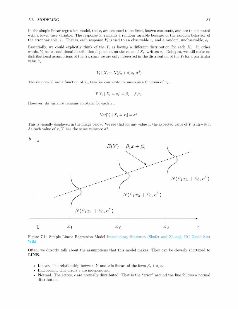
7.1. MODELING 81
In the simple linear regression model, the xi are assumed to be fixed, known constants, and are thus notatedwith a lower case variable. The response Yi remains a random variable because of the random behavior ofthe error variable, ϵi. That is, each response Yi is tied to an observable xi and a random, unobservable, ϵi.
Essentially, we could explicitly think of the Yi as having a different distribution for each Xi. In otherwords, Yi has a conditional distribution dependent on the value of Xi, written xi. Doing so, we still make nodistributional assumptions of the Xi, since we are only interested in the distribution of the Yi for a particularvalue xi.
Yi | Xi ∼ N(β0 + β1xi, σ2)
The random Yi are a function of xi, thus we can write its mean as a function of xi,
E[Yi | Xi = xi] = β0 + β1xi.
However, its variance remains constant for each xi,
Var[Yi | Xi = xi] = σ2.
This is visually displayed in the image below. We see that for any value x, the expected value of Y is β0 +β1x.At each value of x, Y has the same variance σ2.
Figure 7.1: Simple Linear Regression Model Introductory Statistics (Shafer and Zhang), UC David StatWiki
Often, we directly talk about the assumptions that this model makes. They can be cleverly shortened toLINE.
• Linear. The relationship between Y and x is linear, of the form β0 + β1x.• Indepedent. The errors ϵ are independent.• Normal. The errors, ϵ are normally distributed. That is the “error” around the line follows a normal
distribution.

82 CHAPTER 7. SIMPLE LINEAR REGRESSION
• Equal Variance. At each value of x, the variance of Y is the same, σ2.
We are also assuming that the values of x are fixed, that is, not random. We do not make a distributionalassumption about the predictor variable.
As a side note, we will often refer to simple linear regression as SLR. Some explanation of the name SLR:
• Simple refers to the fact that we are using a single predictor variable. Later we will use multiplepredictor variables.
• Linear tells us that our model for Y is a linear combination of the predictors X. (In this case justthe one.) Right now, this always results in a model that is a line, but later we will see how this is notalways the case.
• Regression simply means that we are attempting to measure the relationship between a responsevariable and (one or more) predictor variables. In the case of SLR, both the response and the predictorare numeric variables.
So SLR models Y as a linear function of X, but how do we actually define a good line? There are an infinitenumber of lines we could use, so we will attempt to find one with “small errors.” That is a line with as manypoints as close to it as possible. The questions now becomes, how do we find such a line? There are manyapproaches we could take.
We could find the line that has the smallest maximum distance from any of the points to the line. That is,
argminβ0,β1
max |yi − (β0 + β1xi)|.
We could find the line that minimizes the sum of all the distances from the points to the line. That is,
argminβ0,β1
n∑i=1
|yi − (β0 + β1xi)|.
We could find the line that minimizes the sum of all the squared distances from the points to the line. Thatis,
argminβ0,β1
n∑i=1
(yi − (β0 + β1xi))2.
This last option is called the method of least squares. It is essentially the de-facto method for fitting aline to data. (You may have even seen it before in a linear algebra course.) Its popularity is largely dueto the fact that it is mathematically “easy.” (Which was important historically, as computers are a moderncontraption.) It is also very popular because many relationships are well approximated by a linear function.
7.2 Least Squares Approach
Given observations (xi, yi), for i = 1, 2, . . . n, we want to find values of β0 and β1 which minimize
f(β0, β1) =n∑
i=1(yi − (β0 + β1xi))2 =
n∑i=1
(yi − β0 − β1xi)2.
We will call these values β0 and β1.
7.2. LEAST SQUARES APPROACH 83
First, we take a partial derivative with respect to both β0 and β1.
∂f
∂β0= −2
n∑i=1
(yi − β0 − β1xi)
∂f
∂β1= −2
n∑i=1
(xi)(yi − β0 − β1xi)
We then set each of the partial derivatives equal to zero and solving the resulting system of equations.
n∑i=1
(yi − β0 − β1xi) = 0
n∑i=1
(xi)(yi − β0 − β1xi) = 0
While solving the system of equations, one common algebraic rearrangement results in the normal equa-tions.
nβ0 + β1
n∑i=1
xi =n∑
i=1yi
β0
n∑i=1
xi + β1
n∑i=1
x2i =
n∑i=1
xiyi
Finally, we finish solving the system of equations.
β1 =∑n
i=1 xiyi −(∑n
i=1xi)(∑n
i=1yi)
n∑ni=1 x2
i −(∑n
i=1xi)2
n
= Sxy
Sxx
β0 = y − β1x
Here, we have defined some notation for the expression we’ve obtained. Note that they have alternativeforms which are much easier to work with. (We won’t do it here, but you can try to prove the equalitiesbelow on your own, for “fun.”) We use the capital letter S to denote “summation” which replaces the capitalletter Σ when we calculate these values based on observed data, (xi, yi). The subscripts such as xy denoteover which variables the function (z − z) is applied.
Sxy =n∑
i=1xiyi −
(∑n
i=1 xi)(∑n
i=1 yi)n
=n∑
i=1(xi − x)(yi − y)
Sxx =n∑
i=1x2
i −(∑n
i=1 xi)2
n=
n∑i=1
(xi − x)2
Syy =n∑
i=1y2
i −(∑n
i=1 yi)2
n=
n∑i=1
(yi − y)2
Note that these summations S are not to be confused with sample standard deviation s.
By using the above alternative expressions for Sxy and Sxx, we arrive at a cleaner, more useful expressionfor β1.
84 CHAPTER 7. SIMPLE LINEAR REGRESSION
β1 = Sxy
Sxx=∑n
i=1(xi − x)(yi − y)∑ni=1(xi − x)2
Traditionally we would now calculate β0 and β1 by hand for the cars dataset. However because we are livingin the 21st century and are intelligent (or lazy or efficient, depending on your perspective), we will utilize Rto do the number crunching for us.
To keep some notation consistent with above mathematics, we will store the response variable as y and thepredictor variable as x.
x = cars$speedy = cars$dist
We then calculate the three sums of squares defined above.
Sxy = sum((x - mean(x)) * (y - mean(y)))Sxx = sum((x - mean(x)) ^ 2)Syy = sum((y - mean(y)) ^ 2)c(Sxy, Sxx, Syy)
## [1] 5387.40 1370.00 32538.98
Then finally calculate β0 and β1.
beta_1_hat = Sxy / Sxxbeta_0_hat = mean(y) - beta_1_hat * mean(x)c(beta_0_hat, beta_1_hat)
## [1] -17.579095 3.932409
What do these values tell us about our dataset?
The slope parameter β1 tells us that for an increase in speed of one mile per hour, the mean stoppingdistance increases by β1. It is important to specify that we are talking about the mean. Recall that β0 +β1xis the estimated mean of Y , in this case stopping distance, for a particular value of x. (In this case speed.)So β1 tells us how the mean of Y is affected by a change in x.
Similarly, the estimate β1 = 3.93 tells us that for an increase in speed of one mile per hour, the estimatedmean stopping distance increases by 3.93 feet. Here we should be sure to specify we are discussing anestimated quantity. Recall that y is the estimated mean of Y , so β1 tells us how the estimated mean of Yis affected by changing x.
The intercept parameter β0 tells us the mean stopping distance for a car traveling zero miles per hour. (Notmoving.) The estimate β0 = −17.58 tells us that the estimated mean stopping distance for a car travelingzero miles per hour is −17.58 feet. So when you apply the brakes to a car that is not moving, it movesbackwards? This doesn’t seem right. (Extrapolation, which we will see later, is the issue here.)
7.2.1 Making Predictions
We can now write the fitted or estimated line,
y = β0 + β1x.

7.2. LEAST SQUARES APPROACH 85
In this case,
y = −17.58 + 3.93x.
We can now use this line to make predictions. First, let’s see the possible x values in the cars dataset. Sincesome x values may appear more than once, we use the unique() to return each unique value only once.
unique(cars$speed)
## [1] 4 7 8 9 10 11 12 13 14 15 16 17 18 19 20 22 23 24 25
Let’s make a prediction for the stopping distance of a car traveling at 8 miles per hour.
y = −17.58 + 3.93 × 8
beta_0_hat + beta_1_hat * 8
## [1] 13.88018
This tells us that the estimated mean stopping distance of a car traveling at 8 miles per hour is 13.88.
Now let’s make a prediction for the stopping distance of a car traveling at 21 miles per hour. This isconsidered interpolation as 21 is not an observed value of x. (But is in the data range.) We can use thespecial %in% operator to quickly verify this in R.
8 %in% unique(cars$speed)
## [1] TRUE
21 %in% unique(cars$speed)
## [1] FALSE
min(cars$speed) < 21 & 21 < max(cars$speed)
## [1] TRUE
y = −17.58 + 3.93 × 21
beta_0_hat + beta_1_hat * 21
## [1] 65.00149
Lastly, we can make a prediction for the stopping distance of a car traveling at 50 miles per hour. This isconsidered extrapolation as 50 is not an observed value of x and is outside data range. We should be lessconfident in predictions of this type.

86 CHAPTER 7. SIMPLE LINEAR REGRESSION
range(cars$speed)
## [1] 4 25
range(cars$speed)[1] < 50 & 50 < range(cars$speed)[2]
## [1] FALSE
y = −17.58 + 3.93 × 50
beta_0_hat + beta_1_hat * 50
## [1] 179.0413
Cars travel 50 miles per hour rather easily today, but not in the 1920s!This is also an issue we saw when interpreting β0 = −17.58, which is equivalent to making a prediction atx = 0. We should not be confident in the estimated linear relationship outside of the range of data we haveobserved.
7.2.2 Residuals
If we think of our model as “Response = Prediction + Error,” we can then write it as
y = y + e.
We then define a residual to be the observed value minus the predicted value.
ei = yi − yi
Let’s calculate the residual for the prediction we made for a car traveling 8 miles per hour. First, we needto obtain the observed value of y for this x value.
which(cars$speed == 8)
## [1] 5
cars[5, ]
## speed dist## 5 8 16
cars[which(cars$speed == 8), ]
## speed dist## 5 8 16
We can then calculate the residual.
e = 16 − 13.88 = 2.12
7.2. LEAST SQUARES APPROACH 87
16 - (beta_0_hat + beta_1_hat * 8)
## [1] 2.119825
The positive residual value indicates that the observed stopping distance is actually 2.12 feet more than whatwas predicted.
7.2.3 Variance Estimation
We’ll now use the residuals for each of the points to create an estimate for the variance, σ2.
Recall that,
E[Yi | Xi = xi] = β0 + β1xi.
So,
yi = β0 + β1xi
is a natural estimate for the mean of Yi for a given value of xi.
Also, recall that when we specified the model, we had three unknown parameters; β0, β1, and σ2. Themethod of least squares gave us estimates for β0 and β1, however, we have yet to see an estimate for σ2. Wewill now define s2
e which will be an estimate for σ2.
s2e = 1
n − 2
n∑i=1
(yi − (β0 + β1xi))2
= 1n − 2
n∑i=1
(yi − yi)2
= 1n − 2
n∑i=1
e2i
This probably seems like a natural estimate, aside from the use of n − 2, which we will put off explaininguntil the next chapter. It should actually look rather similar to something we have seen before.
s2 = 1n − 1
n∑i=1
(xi − x)2
Here, s2 is the estimate of σ2 when we have a single random variable X. In this case x is an estimate of µwhich is assumed to be the same for each x.
Now, in the regression case, with s2e each y has a different mean because of the relationship with x. Thus,
for each yi, we use a different estimate of the mean, that is yi.
y_hat = beta_0_hat + beta_1_hat * xe = y - y_hatn = length(e)s2_e = sum(e^2) / (n - 2)s2_e
88 CHAPTER 7. SIMPLE LINEAR REGRESSION
## [1] 236.5317
Just as with the univariate measure of variance, this value of 236.53 doesn’t have a practical interpretationin terms of stopping distance. Taking the square root, however, computes the standard deviation of theresiduals, also known as residual standard error.
s_e = sqrt(s2_e)s_e
## [1] 15.37959
This tells us that our estimates of mean stopping distance are “typically” off by 15.38 feet.
7.3 Decomposition of Variation
We can re-express yi − y, which measures the deviation of an observation from the sample mean, in thefollowing way,
yi − y = (yi − yi) + (yi − y).
This is the common mathematical trick of “adding zero.” In this case we both added and subtracted yi.Here, yi − yi measures the deviation of an observation from the fitted regression line and yi − y measuresthe deviation of the fitted regression line from the sample mean.If we square then sum both sides of the equation above, we can obtain the following,
n∑i=1
(yi − y)2 =n∑
i=1(yi − yi)2 +
n∑i=1
(yi − y)2.
This should be somewhat alarming or amazing. How is this true? For now we will leave this questionsunanswered. (Think about this, and maybe try to prove it.) We will now define three of the quantities seenin this equation.
Sum of Squares Total
SST =n∑
i=1(yi − y)2
The quantity “Sum of Squares Total,” or SST, represents the total variation of the observed y values. Thisshould be a familiar looking expression. Note that,
s2 = 1n − 1
n∑i=1
(yi − y)2 = 1n − 1
SST.
Sum of Squares Regression
SSReg =n∑
i=1(yi − y)2
The quantity “Sum of Squares Regression,” SSReg, represents the explained variation of the observed yvalues.
7.3. DECOMPOSITION OF VARIATION 89
Sum of Squares Error
SSE = RSS =n∑
i=1(yi − yi)2
The quantity “Sum of Squares Error,” SSE, represents the unexplained variation of the observed y values.You will often see SSE written as RSS, or “Residual Sum of Squares.”
SST = sum((y - mean(y)) ^ 2)SSReg = sum((y_hat - mean(y)) ^ 2)SSE = sum((y - y_hat) ^ 2)c(SST = SST, SSReg = SSReg, SSE = SSE)
## SST SSReg SSE## 32538.98 21185.46 11353.52
Note that,
s2e = SSE
n − 2.
SSE / (n - 2)
## [1] 236.5317
We can use R to verify that this matches our previous calculation of s2e.
s2_e == SSE / (n - 2)
## [1] TRUE
These three measures also do not have an important practical interpretation individually. But together,they’re about to reveal a new statistic to help measure the strength of a SLR model.
7.3.1 Coefficient of Determination
The coefficient of determination, R2, is defined as
R2 = SSRegSST =
∑ni=1(yi − y)2∑ni=1(yi − y)2
= SST − SSESST = 1 − SSE
SST
= 1 −∑n
i=1(yi − yi)2∑ni=1(yi − y)2 = 1 −
∑ni=1 e2
i∑ni=1(yi − y)2
The coefficient of determination is interpreted as the proportion of observed variation in y that can beexplained by the simple linear regression model.
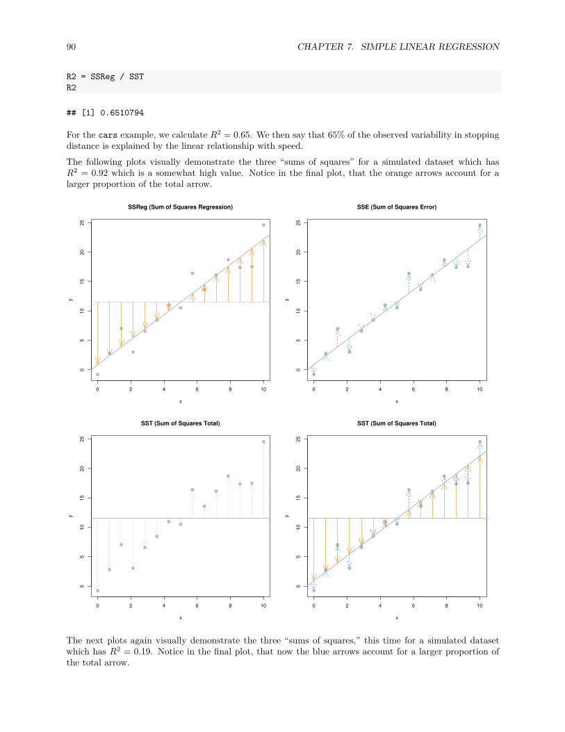
90 CHAPTER 7. SIMPLE LINEAR REGRESSION
R2 = SSReg / SSTR2
## [1] 0.6510794
For the cars example, we calculate R2 = 0.65. We then say that 65% of the observed variability in stoppingdistance is explained by the linear relationship with speed.The following plots visually demonstrate the three “sums of squares” for a simulated dataset which hasR2 = 0.92 which is a somewhat high value. Notice in the final plot, that the orange arrows account for alarger proportion of the total arrow.
0 2 4 6 8 10
05
1015
2025
SSReg (Sum of Squares Regression)
x
y
0 2 4 6 8 10
05
1015
2025
SSE (Sum of Squares Error)
x
y
0 2 4 6 8 10
05
1015
2025
SST (Sum of Squares Total)
x
y
0 2 4 6 8 10
05
1015
2025
SST (Sum of Squares Total)
x
y
The next plots again visually demonstrate the three “sums of squares,” this time for a simulated datasetwhich has R2 = 0.19. Notice in the final plot, that now the blue arrows account for a larger proportion ofthe total arrow.
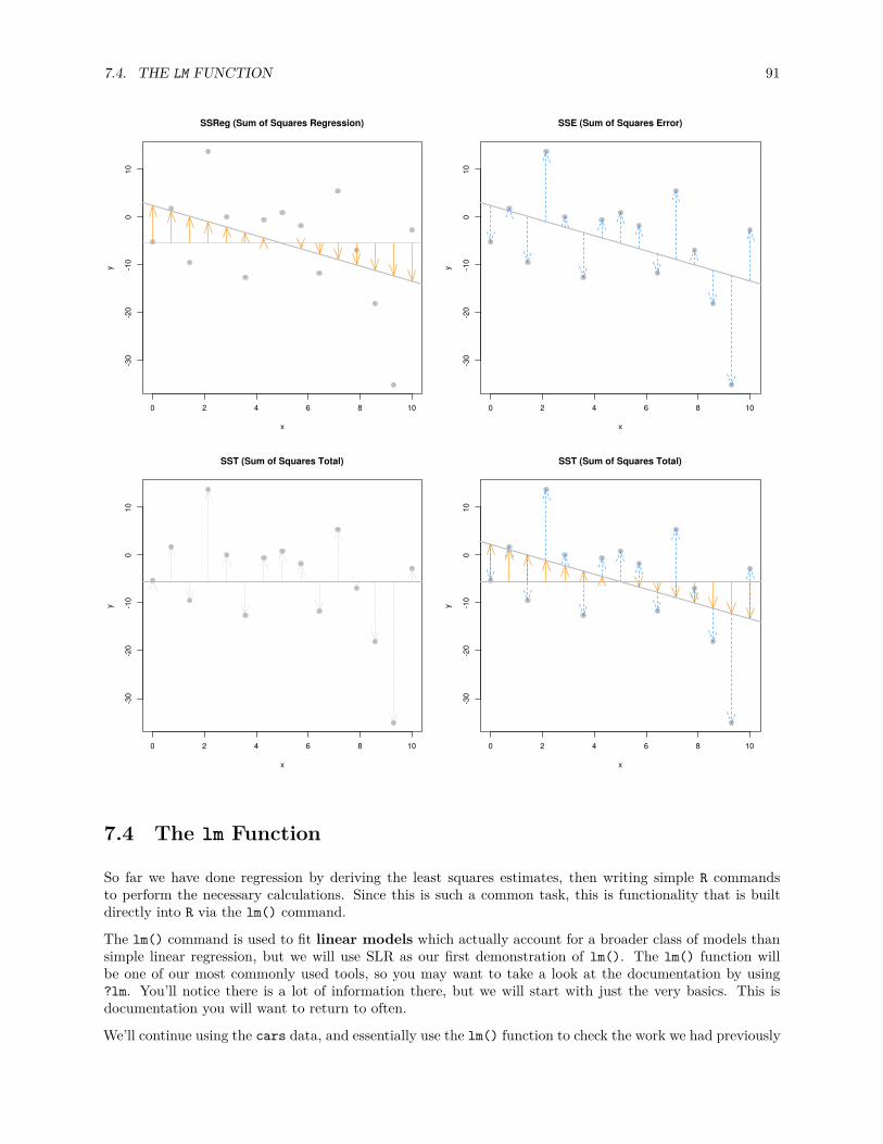
7.4. THE LM FUNCTION 91
0 2 4 6 8 10
-30
-20
-10
010
SSReg (Sum of Squares Regression)
x
y
0 2 4 6 8 10
-30
-20
-10
010
SSE (Sum of Squares Error)
x
y
0 2 4 6 8 10
-30
-20
-10
010
SST (Sum of Squares Total)
x
y
0 2 4 6 8 10
-30
-20
-10
010
SST (Sum of Squares Total)
x
y
7.4 The lm Function
So far we have done regression by deriving the least squares estimates, then writing simple R commandsto perform the necessary calculations. Since this is such a common task, this is functionality that is builtdirectly into R via the lm() command.
The lm() command is used to fit linear models which actually account for a broader class of models thansimple linear regression, but we will use SLR as our first demonstration of lm(). The lm() function willbe one of our most commonly used tools, so you may want to take a look at the documentation by using?lm. You’ll notice there is a lot of information there, but we will start with just the very basics. This isdocumentation you will want to return to often.
We’ll continue using the cars data, and essentially use the lm() function to check the work we had previously

92 CHAPTER 7. SIMPLE LINEAR REGRESSION
done.
stop_dist_model = lm(dist ~ speed, data = cars)
This line of code fits our very first linear model. The syntax should look somewhat familiar. We use thedist ~ speed syntax to tell R we would like to model the response variable dist as a linear function of thepredictor variable speed. In general, you should think of the syntax as response ~ predictor. The data= cars argument then tells R that that dist and speed variables are from the dataset cars. We then storethis result in a variable stop_dist_model.
The variable stop_dist_model now contains a wealth of information, and we will now see how to extractand use that information. The first thing we will do is simply output whatever is stored immediately in thevariable stop_dist_model.
stop_dist_model
#### Call:## lm(formula = dist ~ speed, data = cars)#### Coefficients:## (Intercept) speed## -17.579 3.932
We see that it first tells us the formula we input into R, that is lm(formula = dist ~ speed, data =cars). We also see the coefficients of the model. We can check that these are what we had calculatedpreviously. (Minus some rounding that R is doing when displaying the results. They are stored with fullprecision.)
c(beta_0_hat, beta_1_hat)
## [1] -17.579095 3.932409
Next, it would be nice to add the fitted line to the scatterplot. To do so we will use the abline() function.
plot(dist ~ speed, data = cars,xlab = "Speed (in Miles Per Hour)",ylab = "Stopping Distance (in Feet)",main = "Stopping Distance vs Speed",pch = 20,cex = 2,col = "grey")
abline(stop_dist_model, lwd = 3, col = "darkorange")
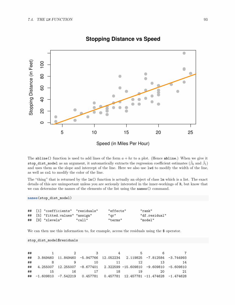
7.4. THE LM FUNCTION 93
5 10 15 20 25
020
4060
8010
0Stopping Distance vs Speed
Speed (in Miles Per Hour)
Sto
ppin
g D
ista
nce
(in F
eet)
The abline() function is used to add lines of the form a + bx to a plot. (Hence abline.) When we give itstop_dist_model as an argument, it automatically extracts the regression coefficient estimates (β0 and β1)and uses them as the slope and intercept of the line. Here we also use lwd to modify the width of the line,as well as col to modify the color of the line.
The “thing” that is returned by the lm() function is actually an object of class lm which is a list. The exactdetails of this are unimportant unless you are seriously interested in the inner-workings of R, but know thatwe can determine the names of the elements of the list using the names() command.
names(stop_dist_model)
## [1] "coefficients" "residuals" "effects" "rank"## [5] "fitted.values" "assign" "qr" "df.residual"## [9] "xlevels" "call" "terms" "model"
We can then use this information to, for example, access the residuals using the $ operator.
stop_dist_model$residuals
## 1 2 3 4 5 6 7## 3.849460 11.849460 -5.947766 12.052234 2.119825 -7.812584 -3.744993## 8 9 10 11 12 13 14## 4.255007 12.255007 -8.677401 2.322599 -15.609810 -9.609810 -5.609810## 15 16 17 18 19 20 21## -1.609810 -7.542219 0.457781 0.457781 12.457781 -11.474628 -1.474628
94 CHAPTER 7. SIMPLE LINEAR REGRESSION
## 22 23 24 25 26 27 28## 22.525372 42.525372 -21.407036 -15.407036 12.592964 -13.339445 -5.339445## 29 30 31 32 33 34 35## -17.271854 -9.271854 0.728146 -11.204263 2.795737 22.795737 30.795737## 36 37 38 39 40 41 42## -21.136672 -11.136672 10.863328 -29.069080 -13.069080 -9.069080 -5.069080## 43 44 45 46 47 48 49## 2.930920 -2.933898 -18.866307 -6.798715 15.201285 16.201285 43.201285## 50## 4.268876
Another way to access stored information in stop_dist_model are the coef(), resid(), and fitted()functions. These return the coefficients, residuals, and fitted values, respectively.
coef(stop_dist_model)
## (Intercept) speed## -17.579095 3.932409
resid(stop_dist_model)
## 1 2 3 4 5 6 7## 3.849460 11.849460 -5.947766 12.052234 2.119825 -7.812584 -3.744993## 8 9 10 11 12 13 14## 4.255007 12.255007 -8.677401 2.322599 -15.609810 -9.609810 -5.609810## 15 16 17 18 19 20 21## -1.609810 -7.542219 0.457781 0.457781 12.457781 -11.474628 -1.474628## 22 23 24 25 26 27 28## 22.525372 42.525372 -21.407036 -15.407036 12.592964 -13.339445 -5.339445## 29 30 31 32 33 34 35## -17.271854 -9.271854 0.728146 -11.204263 2.795737 22.795737 30.795737## 36 37 38 39 40 41 42## -21.136672 -11.136672 10.863328 -29.069080 -13.069080 -9.069080 -5.069080## 43 44 45 46 47 48 49## 2.930920 -2.933898 -18.866307 -6.798715 15.201285 16.201285 43.201285## 50## 4.268876
fitted(stop_dist_model)
## 1 2 3 4 5 6 7 8## -1.849460 -1.849460 9.947766 9.947766 13.880175 17.812584 21.744993 21.744993## 9 10 11 12 13 14 15 16## 21.744993 25.677401 25.677401 29.609810 29.609810 29.609810 29.609810 33.542219## 17 18 19 20 21 22 23 24## 33.542219 33.542219 33.542219 37.474628 37.474628 37.474628 37.474628 41.407036## 25 26 27 28 29 30 31 32## 41.407036 41.407036 45.339445 45.339445 49.271854 49.271854 49.271854 53.204263## 33 34 35 36 37 38 39 40## 53.204263 53.204263 53.204263 57.136672 57.136672 57.136672 61.069080 61.069080## 41 42 43 44 45 46 47 48## 61.069080 61.069080 61.069080 68.933898 72.866307 76.798715 76.798715 76.798715

7.4. THE LM FUNCTION 95
## 49 50## 76.798715 80.731124
An R function that is useful in many situations is summary(). We see that when it is called on our model, itreturns a good deal of information. By the end of the course, you will know what every value here is usedfor. For now, you should immediately notice the coefficient estimates, and you may recognize the R2 valuewe saw earlier.
summary(stop_dist_model)
#### Call:## lm(formula = dist ~ speed, data = cars)#### Residuals:## Min 1Q Median 3Q Max## -29.069 -9.525 -2.272 9.215 43.201#### Coefficients:## Estimate Std. Error t value Pr(>|t|)## (Intercept) -17.5791 6.7584 -2.601 0.0123 *## speed 3.9324 0.4155 9.464 1.49e-12 ***## ---## Signif. codes: 0 '***' 0.001 '**' 0.01 '*' 0.05 '.' 0.1 ' ' 1#### Residual standard error: 15.38 on 48 degrees of freedom## Multiple R-squared: 0.6511, Adjusted R-squared: 0.6438## F-statistic: 89.57 on 1 and 48 DF, p-value: 1.49e-12
The summary() command also returns a list, and we can again use names() to learn what about the elementsof this list.
names(summary(stop_dist_model))
## [1] "call" "terms" "residuals" "coefficients"## [5] "aliased" "sigma" "df" "r.squared"## [9] "adj.r.squared" "fstatistic" "cov.unscaled"
So, for example, if we wanted to directly access the value of R2, instead of copy and pasting it out of theprinted statement from summary(), we could do so.
summary(stop_dist_model)$r.squared
## [1] 0.6510794
Another value we may want to access is se, which R calls sigma.
summary(stop_dist_model)$sigma
## [1] 15.37959

96 CHAPTER 7. SIMPLE LINEAR REGRESSION
Note that this is the same result seen earlier as s_e. You may also notice that this value was displayed aboveas a result of the summary() command, which R labeled the “Residual Standard Error.”
se = RSE =
√√√√ 1n − 2
n∑i=1
e2i
Often it is useful to talk about se (or RSE) instead of s2e because of their units. The units of se in the cars
example is feet, while the units of s2e is feet-squared.
Another useful function, which we will use almost as often as lm() is the predict() function.
predict(stop_dist_model, newdata = data.frame(speed = 8))
## 1## 13.88018
The above code reads “predict the stopping distance of a car traveling 8 miles per hour using thestop_dist_model.” Importantly, the second argument to predict() is a data frame that we make in place.We do this so that we can specify that 8 is a value of speed, so that predict knows how to use it with themodel stored in stop_dist_model. We see that this result is what we had calculated “by hand” previously.We could also predict multiple values at once.
predict(stop_dist_model, newdata = data.frame(speed = c(8, 21, 50)))
## 1 2 3## 13.88018 65.00149 179.04134
y = −17.58 + 3.93 × 8 = 13.88y = −17.58 + 3.93 × 21 = 65y = −17.58 + 3.93 × 50 = 179.04
Or we could calculate the fitted value for each of the original data points. We can simply supply the originaldata frame, cars, since it contains a variables called speed which has the values we would like to predict at.
predict(stop_dist_model, newdata = cars)
## 1 2 3 4 5 6 7 8## -1.849460 -1.849460 9.947766 9.947766 13.880175 17.812584 21.744993 21.744993## 9 10 11 12 13 14 15 16## 21.744993 25.677401 25.677401 29.609810 29.609810 29.609810 29.609810 33.542219## 17 18 19 20 21 22 23 24## 33.542219 33.542219 33.542219 37.474628 37.474628 37.474628 37.474628 41.407036## 25 26 27 28 29 30 31 32## 41.407036 41.407036 45.339445 45.339445 49.271854 49.271854 49.271854 53.204263## 33 34 35 36 37 38 39 40## 53.204263 53.204263 53.204263 57.136672 57.136672 57.136672 61.069080 61.069080## 41 42 43 44 45 46 47 48## 61.069080 61.069080 61.069080 68.933898 72.866307 76.798715 76.798715 76.798715## 49 50## 76.798715 80.731124

7.5. MAXIMUM LIKELIHOOD ESTIMATION (MLE) APPROACH 97
# predict(stop_dist_model, newdata = data.frame(speed = cars$speed))
This is actually equivalent to simply calling predict() on stop_dist_model without a second argument.
predict(stop_dist_model)
## 1 2 3 4 5 6 7 8## -1.849460 -1.849460 9.947766 9.947766 13.880175 17.812584 21.744993 21.744993## 9 10 11 12 13 14 15 16## 21.744993 25.677401 25.677401 29.609810 29.609810 29.609810 29.609810 33.542219## 17 18 19 20 21 22 23 24## 33.542219 33.542219 33.542219 37.474628 37.474628 37.474628 37.474628 41.407036## 25 26 27 28 29 30 31 32## 41.407036 41.407036 45.339445 45.339445 49.271854 49.271854 49.271854 53.204263## 33 34 35 36 37 38 39 40## 53.204263 53.204263 53.204263 57.136672 57.136672 57.136672 61.069080 61.069080## 41 42 43 44 45 46 47 48## 61.069080 61.069080 61.069080 68.933898 72.866307 76.798715 76.798715 76.798715## 49 50## 76.798715 80.731124
Note that then in this case, this is the same as using fitted().
fitted(stop_dist_model)
## 1 2 3 4 5 6 7 8## -1.849460 -1.849460 9.947766 9.947766 13.880175 17.812584 21.744993 21.744993## 9 10 11 12 13 14 15 16## 21.744993 25.677401 25.677401 29.609810 29.609810 29.609810 29.609810 33.542219## 17 18 19 20 21 22 23 24## 33.542219 33.542219 33.542219 37.474628 37.474628 37.474628 37.474628 41.407036## 25 26 27 28 29 30 31 32## 41.407036 41.407036 45.339445 45.339445 49.271854 49.271854 49.271854 53.204263## 33 34 35 36 37 38 39 40## 53.204263 53.204263 53.204263 57.136672 57.136672 57.136672 61.069080 61.069080## 41 42 43 44 45 46 47 48## 61.069080 61.069080 61.069080 68.933898 72.866307 76.798715 76.798715 76.798715## 49 50## 76.798715 80.731124
7.5 Maximum Likelihood Estimation (MLE) Approach
Recall the model,
Yi = β0 + β1xi + ϵi
where ϵi ∼ N(0, σ2).
Then we can find the mean and variance of each Yi.

98 CHAPTER 7. SIMPLE LINEAR REGRESSION
E[Yi | Xi = xi] = β0 + β1xi
and
Var[Yi | Xi = xi] = σ2.
Addtionaly, the Yi follow a normal distribution conditioned on the xi.
Yi | Xi ∼ N(β0 + β1xi, σ2)
Recall that the pdf of a random variable X ∼ N(µ, σ2) is given by
fX(x; µ, σ2) = 1√2πσ2
exp
[−1
2
(x − µ
σ
)2]
.
Then we can write the pdf of each of the Yi as
fYi(yi; xi, β0, β1, σ2) = 1√
2πσ2exp
[−1
2
(yi − (β0 + β1xi)
σ
)2]
.
Given n data points (xi, yi) we can write the likelihood, which is a function of the three parameters β0, β1,and σ2. Since the data have been observed, we use lower case yi to denote that these values are no longerrandom.
L(β0, β1, σ2) =n∏
i=1
1√2πσ2
exp
[−1
2
(yi − β0 − β1xi
σ
)2]
Our goal is to find values of β0, β1, and σ2 which maximize this function, which is a straightforwardmultivariate calculus problem.
We’ll start by doing a bit of rearranging to make our task easier.
L(β0, β1, σ2) =(
1√2πσ2
)n
exp
[− 1
2σ2
n∑i=1
(yi − β0 − β1xi)2
]
Then, as is often the case when finding MLEs, for mathematical convenience we will take the naturallogarithm of the likelihood function since log is a monotonically increasing function. Then we will proceedto maximize the log-likelihood, and the resulting estimates will be the same as if we had not taken the log.
log L(β0, β1, σ2) = −n
2log(2π) − n
2log(σ2) − 1
2σ2
n∑i=1
(yi − β0 − β1xi)2
Note that we use log to mean the natural logarithm. We now take a partial derivative with respect to eachof the parameters.
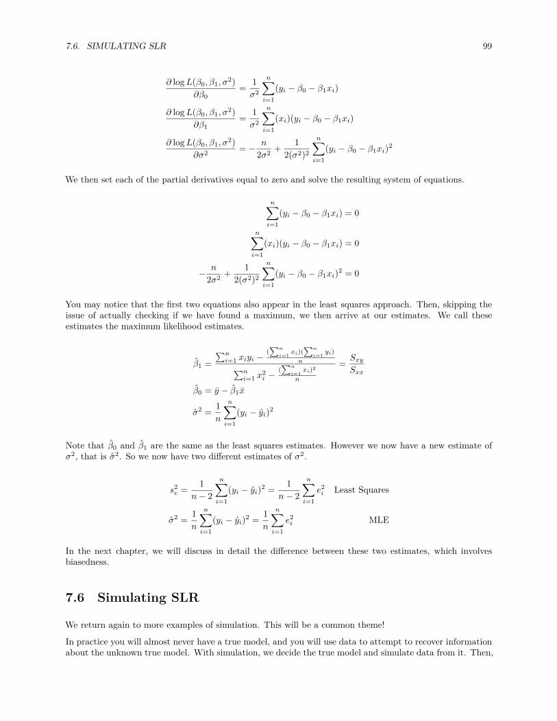
7.6. SIMULATING SLR 99
∂ log L(β0, β1, σ2)∂β0
= 1σ2
n∑i=1
(yi − β0 − β1xi)
∂ log L(β0, β1, σ2)∂β1
= 1σ2
n∑i=1
(xi)(yi − β0 − β1xi)
∂ log L(β0, β1, σ2)∂σ2 = − n
2σ2 + 12(σ2)2
n∑i=1
(yi − β0 − β1xi)2
We then set each of the partial derivatives equal to zero and solve the resulting system of equations.
n∑i=1
(yi − β0 − β1xi) = 0
n∑i=1
(xi)(yi − β0 − β1xi) = 0
− n
2σ2 + 12(σ2)2
n∑i=1
(yi − β0 − β1xi)2 = 0
You may notice that the first two equations also appear in the least squares approach. Then, skipping theissue of actually checking if we have found a maximum, we then arrive at our estimates. We call theseestimates the maximum likelihood estimates.
β1 =∑n
i=1 xiyi −(∑n
i=1xi)(∑n
i=1yi)
n∑ni=1 x2
i −(∑n
i=1xi)2
n
= Sxy
Sxx
β0 = y − β1x
σ2 = 1n
n∑i=1
(yi − yi)2
Note that β0 and β1 are the same as the least squares estimates. However we now have a new estimate ofσ2, that is σ2. So we now have two different estimates of σ2.
s2e = 1
n − 2
n∑i=1
(yi − yi)2 = 1n − 2
n∑i=1
e2i Least Squares
σ2 = 1n
n∑i=1
(yi − yi)2 = 1n
n∑i=1
e2i MLE
In the next chapter, we will discuss in detail the difference between these two estimates, which involvesbiasedness.
7.6 Simulating SLR
We return again to more examples of simulation. This will be a common theme!
In practice you will almost never have a true model, and you will use data to attempt to recover informationabout the unknown true model. With simulation, we decide the true model and simulate data from it. Then,
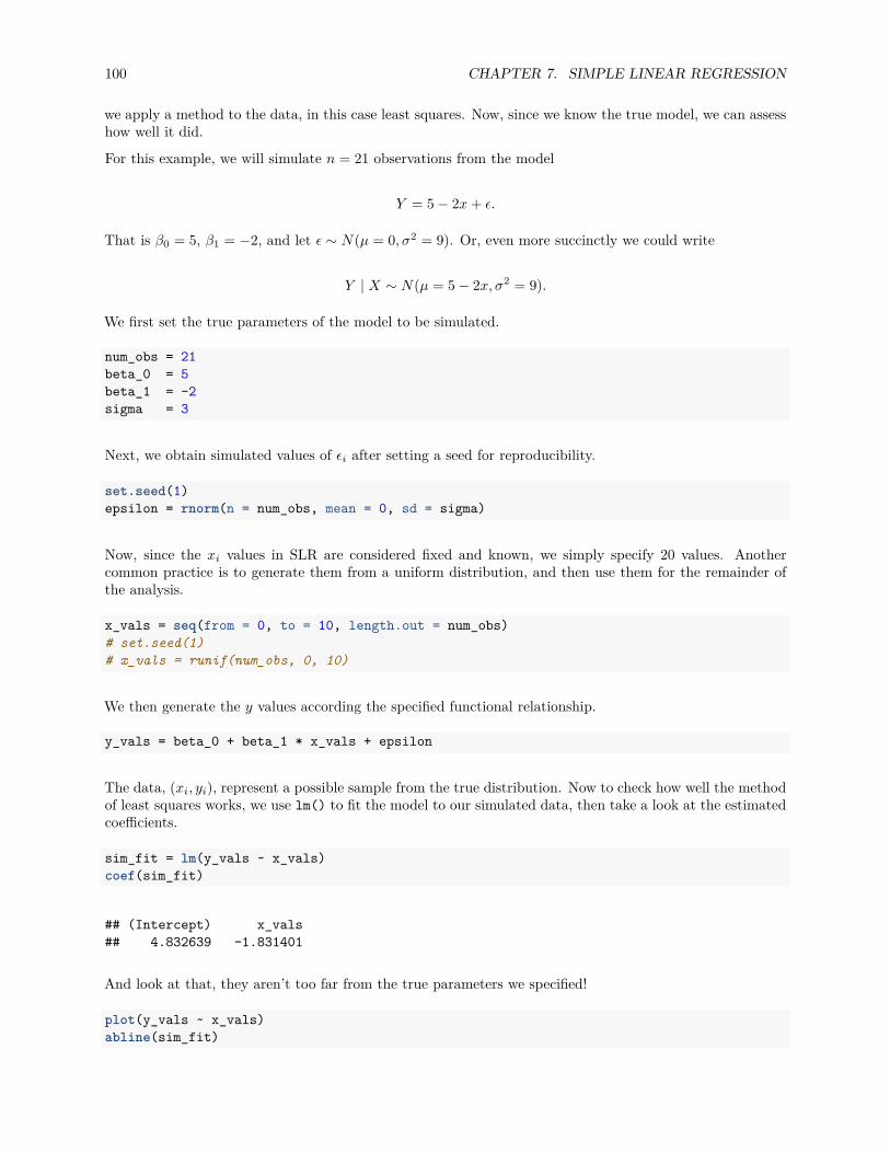
100 CHAPTER 7. SIMPLE LINEAR REGRESSION
we apply a method to the data, in this case least squares. Now, since we know the true model, we can assesshow well it did.
For this example, we will simulate n = 21 observations from the model
Y = 5 − 2x + ϵ.
That is β0 = 5, β1 = −2, and let ϵ ∼ N(µ = 0, σ2 = 9). Or, even more succinctly we could write
Y | X ∼ N(µ = 5 − 2x, σ2 = 9).
We first set the true parameters of the model to be simulated.
num_obs = 21beta_0 = 5beta_1 = -2sigma = 3
Next, we obtain simulated values of ϵi after setting a seed for reproducibility.
set.seed(1)epsilon = rnorm(n = num_obs, mean = 0, sd = sigma)
Now, since the xi values in SLR are considered fixed and known, we simply specify 20 values. Anothercommon practice is to generate them from a uniform distribution, and then use them for the remainder ofthe analysis.
x_vals = seq(from = 0, to = 10, length.out = num_obs)# set.seed(1)# x_vals = runif(num_obs, 0, 10)
We then generate the y values according the specified functional relationship.
y_vals = beta_0 + beta_1 * x_vals + epsilon
The data, (xi, yi), represent a possible sample from the true distribution. Now to check how well the methodof least squares works, we use lm() to fit the model to our simulated data, then take a look at the estimatedcoefficients.
sim_fit = lm(y_vals ~ x_vals)coef(sim_fit)
## (Intercept) x_vals## 4.832639 -1.831401
And look at that, they aren’t too far from the true parameters we specified!
plot(y_vals ~ x_vals)abline(sim_fit)
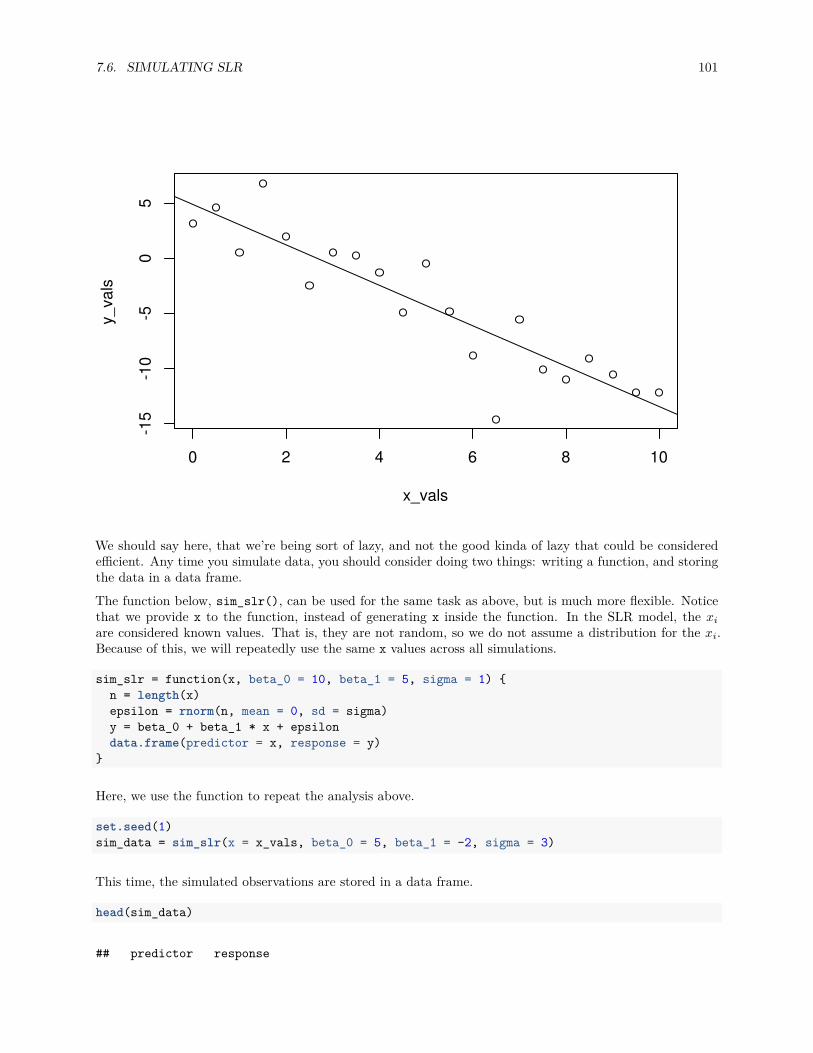
7.6. SIMULATING SLR 101
0 2 4 6 8 10
-15
-10
-50
5
x_vals
y_va
ls
We should say here, that we’re being sort of lazy, and not the good kinda of lazy that could be consideredefficient. Any time you simulate data, you should consider doing two things: writing a function, and storingthe data in a data frame.
The function below, sim_slr(), can be used for the same task as above, but is much more flexible. Noticethat we provide x to the function, instead of generating x inside the function. In the SLR model, the xi
are considered known values. That is, they are not random, so we do not assume a distribution for the xi.Because of this, we will repeatedly use the same x values across all simulations.
sim_slr = function(x, beta_0 = 10, beta_1 = 5, sigma = 1) {n = length(x)epsilon = rnorm(n, mean = 0, sd = sigma)y = beta_0 + beta_1 * x + epsilondata.frame(predictor = x, response = y)
}
Here, we use the function to repeat the analysis above.
set.seed(1)sim_data = sim_slr(x = x_vals, beta_0 = 5, beta_1 = -2, sigma = 3)
This time, the simulated observations are stored in a data frame.
head(sim_data)
## predictor response

102 CHAPTER 7. SIMPLE LINEAR REGRESSION
## 1 0.0 3.1206386## 2 0.5 4.5509300## 3 1.0 0.4931142## 4 1.5 6.7858424## 5 2.0 1.9885233## 6 2.5 -2.4614052
Now when we fit the model with lm() we can use a data argument, a very good practice.
sim_fit = lm(response ~ predictor, data = sim_data)coef(sim_fit)
## (Intercept) predictor## 4.832639 -1.831401
And this time, we’ll make the plot look a lot nicer.
plot(response ~ predictor, data = sim_data,xlab = "Simulated Predictor Variable",ylab = "Simulated Response Variable",main = "Simulated Regression Data",pch = 20,cex = 2,col = "grey")
abline(sim_fit, lwd = 3, lty = 1, col = "darkorange")abline(beta_0, beta_1, lwd = 3, lty = 2, col = "dodgerblue")legend("topright", c("Estimate", "Truth"), lty = c(1, 2), lwd = 2,
col = c("darkorange", "dodgerblue"))
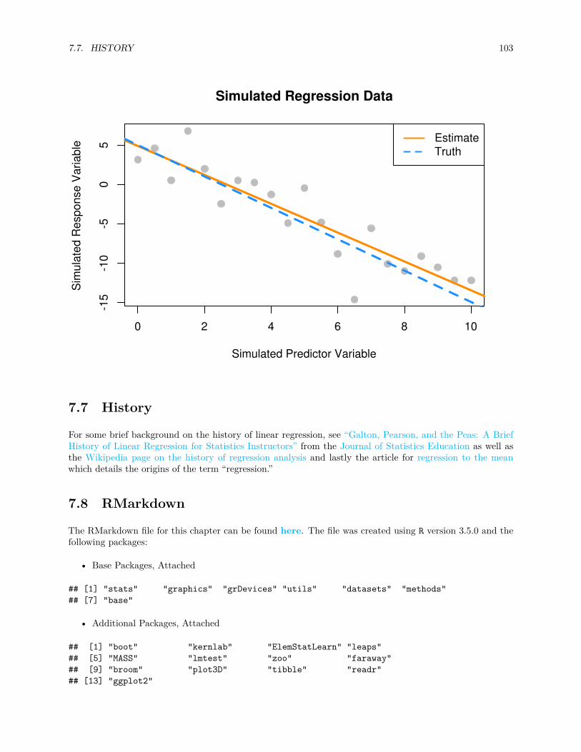
7.7. HISTORY 103
0 2 4 6 8 10
-15
-10
-50
5Simulated Regression Data
Simulated Predictor Variable
Sim
ulat
ed R
espo
nse
Var
iabl
e EstimateTruth
7.7 History
For some brief background on the history of linear regression, see “Galton, Pearson, and the Peas: A BriefHistory of Linear Regression for Statistics Instructors” from the Journal of Statistics Education as well asthe Wikipedia page on the history of regression analysis and lastly the article for regression to the meanwhich details the origins of the term “regression.”
7.8 RMarkdown
The RMarkdown file for this chapter can be found here. The file was created using R version 3.5.0 and thefollowing packages:
• Base Packages, Attached
## [1] "stats" "graphics" "grDevices" "utils" "datasets" "methods"## [7] "base"
• Additional Packages, Attached
## [1] "boot" "kernlab" "ElemStatLearn" "leaps"## [5] "MASS" "lmtest" "zoo" "faraway"## [9] "broom" "plot3D" "tibble" "readr"## [13] "ggplot2"

104 CHAPTER 7. SIMPLE LINEAR REGRESSION
• Additional Packages, Not Attached
## [1] "xfun" "purrr" "reshape2" "splines" "lattice"## [6] "colorspace" "htmltools" "yaml" "utf8" "rlang"## [11] "nloptr" "pillar" "foreign" "glue" "bindrcpp"## [16] "plyr" "bindr" "stringr" "munsell" "gtable"## [21] "codetools" "psych" "evaluate" "labeling" "misc3d"## [26] "knitr" "parallel" "highr" "Rcpp" "scales"## [31] "backports" "lme4" "mnormt" "hms" "digest"## [36] "stringi" "bookdown" "dplyr" "grid" "rprojroot"## [41] "cli" "tools" "magrittr" "lazyeval" "crayon"## [46] "tidyr" "pkgconfig" "Matrix" "minqa" "assertthat"## [51] "rmarkdown" "rstudioapi" "R6" "nlme" "compiler"
Chapter 8
Inference for Simple LinearRegression
“There are three types of lies: lies, damn lies, and statistics.”— Benjamin Disraeli
After reading this chapter you will be able to:
• Understand the distributions of regression estimates.• Create interval estimates for regression parameters, mean response, and predictions.• Test for significance of regression.
Last chapter we defined the simple linear regression model,
Yi = β0 + β1xi + ϵi
where ϵi ∼ N(0, σ2). We then used observations (xi, yi), for i = 1, 2, . . . n, to find values of β0 and β1 whichminimized
f(β0, β1) =n∑
i=1(yi − (β0 + β1xi))2.
We called these values β0 and β1, which we found to be
β1 = Sxy
Sxx=∑n
i=1(xi − x)(yi − y)∑ni=1(xi − x)2
β0 = y − β1x.
We also estimated σ2 using s2e. In other words, we found that se is an estimate of σ, where;
se = RSE =
√√√√ 1n − 2
n∑i=1
e2i
which we also called RSE, for “Residual Standard Error.”When applied to the cars data, we obtained the following results:
105

106 CHAPTER 8. INFERENCE FOR SIMPLE LINEAR REGRESSION
stop_dist_model = lm(dist ~ speed, data = cars)summary(stop_dist_model)
#### Call:## lm(formula = dist ~ speed, data = cars)#### Residuals:## Min 1Q Median 3Q Max## -29.069 -9.525 -2.272 9.215 43.201#### Coefficients:## Estimate Std. Error t value Pr(>|t|)## (Intercept) -17.5791 6.7584 -2.601 0.0123 *## speed 3.9324 0.4155 9.464 1.49e-12 ***## ---## Signif. codes: 0 '***' 0.001 '**' 0.01 '*' 0.05 '.' 0.1 ' ' 1#### Residual standard error: 15.38 on 48 degrees of freedom## Multiple R-squared: 0.6511, Adjusted R-squared: 0.6438## F-statistic: 89.57 on 1 and 48 DF, p-value: 1.49e-12
Last chapter, we only discussed the Estimate, Residual standard error, and Multiple R-squared values.In this chapter, we will discuss all of the information under Coefficients as well as F-statistic.
plot(dist ~ speed, data = cars,xlab = "Speed (in Miles Per Hour)",ylab = "Stopping Distance (in Feet)",main = "Stopping Distance vs Speed",pch = 20,cex = 2,col = "grey")
abline(stop_dist_model, lwd = 5, col = "darkorange")
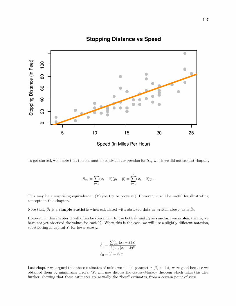
107
5 10 15 20 25
020
4060
8010
0Stopping Distance vs Speed
Speed (in Miles Per Hour)
Sto
ppin
g D
ista
nce
(in F
eet)
To get started, we’ll note that there is another equivalent expression for Sxy which we did not see last chapter,
Sxy =n∑
i=1(xi − x)(yi − y) =
n∑i=1
(xi − x)yi.
This may be a surprising equivalence. (Maybe try to prove it.) However, it will be useful for illustratingconcepts in this chapter.
Note that, β1 is a sample statistic when calculated with observed data as written above, as is β0.
However, in this chapter it will often be convenient to use both β1 and β0 as random variables, that is, wehave not yet observed the values for each Yi. When this is the case, we will use a slightly different notation,substituting in capital Yi for lower case yi.
β1 =∑n
i=1(xi − x)Yi∑ni=1(xi − x)2
β0 = Y − β1x
Last chapter we argued that these estimates of unknown model parameters β0 and β1 were good because weobtained them by minimizing errors. We will now discuss the Gauss–Markov theorem which takes this ideafurther, showing that these estimates are actually the “best” estimates, from a certain point of view.
108 CHAPTER 8. INFERENCE FOR SIMPLE LINEAR REGRESSION
8.1 Gauss–Markov Theorem
The Gauss–Markov theorem tells us that when estimating the parameters of the simple linear regressionmodel β0 and β1, the β0 and β1 which we derived are the best linear unbiased estimates, or BLUE forshort. (The actual conditions for the Gauss–Markov theorem are more relaxed than the SLR model.)
We will now discuss linear, unbiased, and best as is relates to these estimates.
Linear
Recall, in the SLR setup that the xi values are considered fixed and known quantities. Then a linearestimate is one which can be written as a linear combination of the Yi. In the case of β1 we see
β1 =∑n
i=1(xi − x)Yi∑ni=1(xi − x)2 =
n∑i=1
kiYi = k1Y1 + k2Y2 + · · · knYn
where ki = (xi − x)∑ni=1(xi − x)2 .
In a similar fashion, we could show that β0 can be written as a linear combination of the Yi. Thus both β0and β1 are linear estimators.
Unbiased
Now that we know our estimates are linear, how good are these estimates? One measure of the “goodness”of an estimate is its bias. Specifically, we prefer estimates that are unbiased, meaning their expected valueis the parameter being estimated.
In the case of the regression estimates, we have,
E[β0] = β0
E[β1] = β1.
This tells us that, when the conditions of the SLR model are met, on average our estimates will be correct.However, as we saw last chapter when simulating from the SLR model, that does not mean that eachindividual estimate will be correct. Only that, if we repeated the process an infinite number of times, onaverage the estimate would be correct.
Best
Now, if we restrict ourselves to both linear and unbiased estimates, how do we define the best estimate? Theestimate with the minimum variance.
First note that it is very easy to create an estimate for β1 that has very low variance, but is not unbiased.For example, define:
θBAD = 5.
Then, since θBAD is a constant value,
Var[θBAD] = 0.
8.2. SAMPLING DISTRIBUTIONS 109
However since,
E[θBAD] = 5
we say that θBAD is a biased estimator unless β1 = 5, which we would not know ahead of time. For thisreason, it is a terrible estimate (unless by chance β1 = 5) even though it has the smallest possible variance.This is part of the reason we restrict ourselves to unbiased estimates. What good is an estimate, if it estimatesthe wrong quantity?
So now, the natural question is, what are the variances of β0 and β1? They are,
Var[β0] = σ2(
1n
+ x2
Sxx
)Var[β1] = σ2
Sxx.
These quantify the variability of the estimates due to random chance during sampling. Are these “the best”?Are these variances as small as we can possibility get? You’ll just have to take our word for it that they arebecause showing that this is true is beyond the scope of this course.
8.2 Sampling Distributions
Now that we have “redefined” the estimates for β0 and β1 as random variables, we can discuss their samplingdistribution, which is the distribution when a statistic is considered a random variable.
Since both β0 and β1 are a linear combination of the Yi and each Yi is normally distributed, then both β0and β1 also follow a normal distribution.
Then, putting all of the above together, we arrive at the distributions of β0 and β1.
For β1 we say,
β1 = Sxy
Sxx=∑n
i=1(xi − x)Yi∑ni=1(xi − x)2 ∼ N
(β1,
σ2∑ni=1(xi − x)2
).
Or more succinctly,
β1 ∼ N
(β1,
σ2
Sxx
).
And for β0,
β0 = Y − β1x ∼ N
(β0,
σ2∑ni=1 x2
i
n∑n
i=1(xi − x)2
).
Or more succinctly,
β0 ∼ N
(β0, σ2
(1n
+ x2
Sxx
))At this point we have neglected to prove a number of these results. Instead of working through the tediousderivations of these sampling distributions, we will instead justify these results to ourselves using simulation.
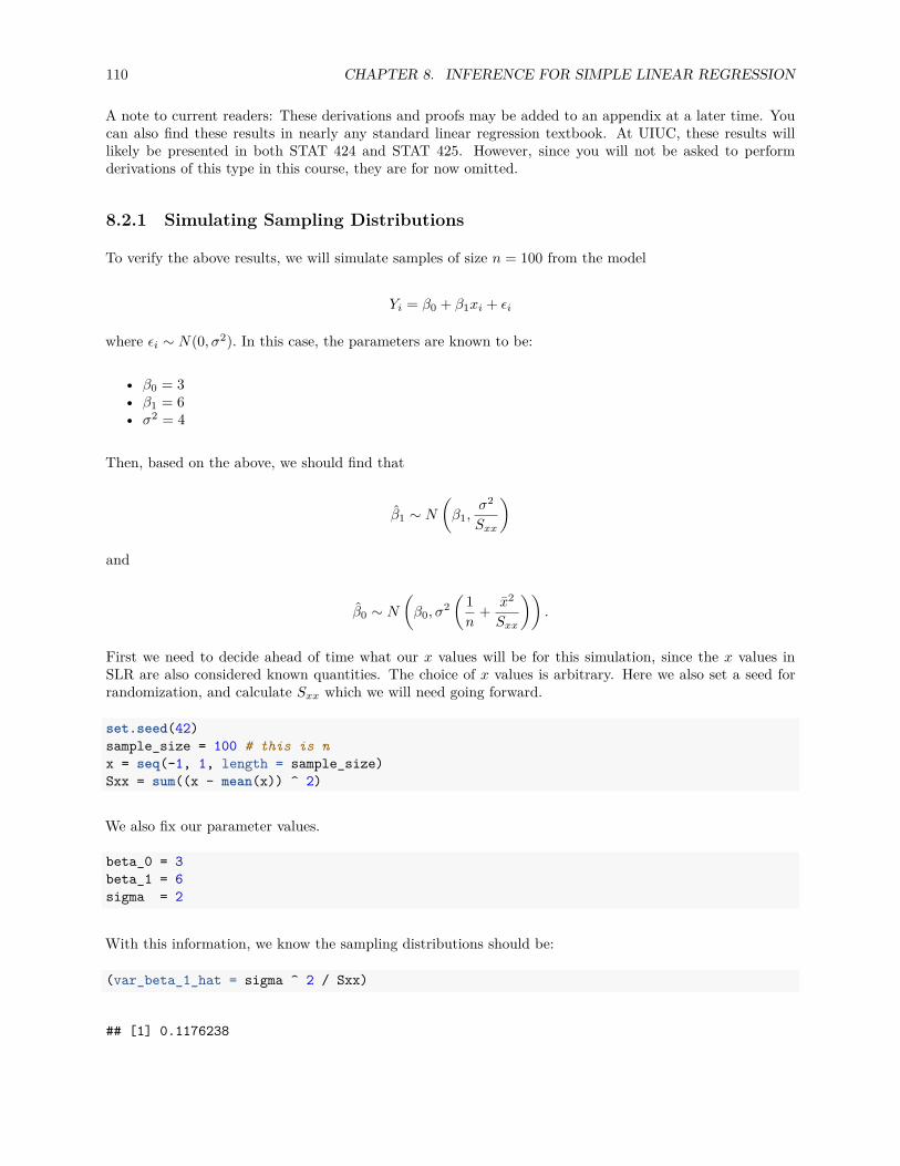
110 CHAPTER 8. INFERENCE FOR SIMPLE LINEAR REGRESSION
A note to current readers: These derivations and proofs may be added to an appendix at a later time. Youcan also find these results in nearly any standard linear regression textbook. At UIUC, these results willlikely be presented in both STAT 424 and STAT 425. However, since you will not be asked to performderivations of this type in this course, they are for now omitted.
8.2.1 Simulating Sampling Distributions
To verify the above results, we will simulate samples of size n = 100 from the model
Yi = β0 + β1xi + ϵi
where ϵi ∼ N(0, σ2). In this case, the parameters are known to be:
• β0 = 3• β1 = 6• σ2 = 4
Then, based on the above, we should find that
β1 ∼ N
(β1,
σ2
Sxx
)and
β0 ∼ N
(β0, σ2
(1n
+ x2
Sxx
)).
First we need to decide ahead of time what our x values will be for this simulation, since the x values inSLR are also considered known quantities. The choice of x values is arbitrary. Here we also set a seed forrandomization, and calculate Sxx which we will need going forward.
set.seed(42)sample_size = 100 # this is nx = seq(-1, 1, length = sample_size)Sxx = sum((x - mean(x)) ^ 2)
We also fix our parameter values.
beta_0 = 3beta_1 = 6sigma = 2
With this information, we know the sampling distributions should be:
(var_beta_1_hat = sigma ^ 2 / Sxx)
## [1] 0.1176238

8.2. SAMPLING DISTRIBUTIONS 111
(var_beta_0_hat = sigma ^ 2 * (1 / sample_size + mean(x) ^ 2 / Sxx))
## [1] 0.04
β1 ∼ N(6, 0.1176238)
and
β0 ∼ N(3, 0.04).
That is,
E[β1] = 6
Var[β1] = 0.1176238
and
E[β0] = 3
Var[β0] = 0.04.
We now simulate data from this model 10,000 times. Note this may not be the most R way of doing thesimulation. We perform the simulation in this manner in an attempt at clarity. For example, we couldhave used the sim_slr() function from the previous chapter. We also simply store variables in the globalenvironment instead of creating a data frame for each new simulated dataset.
num_samples = 10000beta_0_hats = rep(0, num_samples)beta_1_hats = rep(0, num_samples)
for(i in 1:num_samples) {eps = rnorm(sample_size, mean = 0, sd = sigma)y = beta_0 + beta_1 * x + eps
sim_model = lm(y ~ x)
beta_0_hats[i] = coef(sim_model)[1]beta_1_hats[i] = coef(sim_model)[2]
}
Each time we simulated the data, we obtained values of the estimated coefficiets. The variables beta_0_hatsand beta_1_hats now store 10,000 simulated values of β0 and β1 respectively.
We first verify the distribution of β1.
mean(beta_1_hats) # empirical mean
## [1] 6.001998
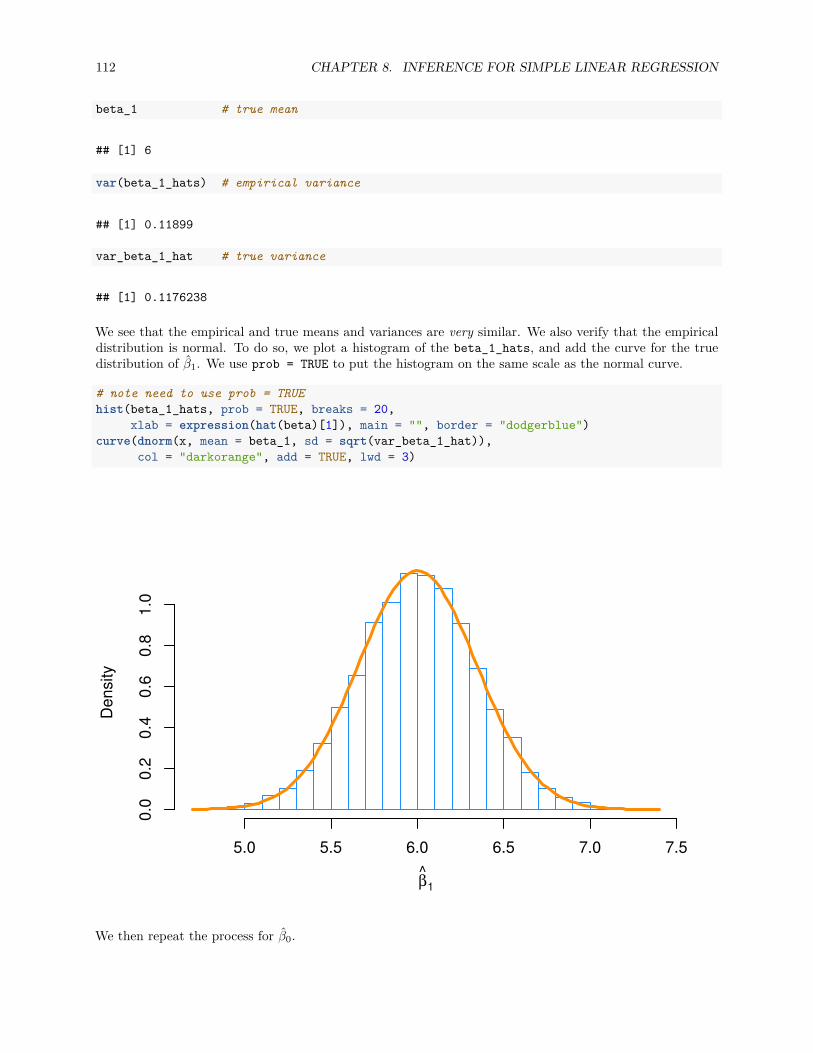
112 CHAPTER 8. INFERENCE FOR SIMPLE LINEAR REGRESSION
beta_1 # true mean
## [1] 6
var(beta_1_hats) # empirical variance
## [1] 0.11899
var_beta_1_hat # true variance
## [1] 0.1176238
We see that the empirical and true means and variances are very similar. We also verify that the empiricaldistribution is normal. To do so, we plot a histogram of the beta_1_hats, and add the curve for the truedistribution of β1. We use prob = TRUE to put the histogram on the same scale as the normal curve.
# note need to use prob = TRUEhist(beta_1_hats, prob = TRUE, breaks = 20,
xlab = expression(hat(beta)[1]), main = "", border = "dodgerblue")curve(dnorm(x, mean = beta_1, sd = sqrt(var_beta_1_hat)),
col = "darkorange", add = TRUE, lwd = 3)
β1
Den
sity
5.0 5.5 6.0 6.5 7.0 7.5
0.0
0.2
0.4
0.6
0.8
1.0
We then repeat the process for β0.
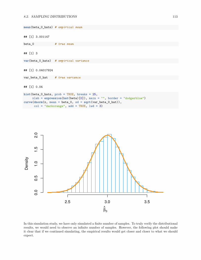
8.2. SAMPLING DISTRIBUTIONS 113
mean(beta_0_hats) # empirical mean
## [1] 3.001147
beta_0 # true mean
## [1] 3
var(beta_0_hats) # empirical variance
## [1] 0.04017924
var_beta_0_hat # true variance
## [1] 0.04
hist(beta_0_hats, prob = TRUE, breaks = 25,xlab = expression(hat(beta)[0]), main = "", border = "dodgerblue")
curve(dnorm(x, mean = beta_0, sd = sqrt(var_beta_0_hat)),col = "darkorange", add = TRUE, lwd = 3)
β0
Den
sity
2.5 3.0 3.5
0.0
0.5
1.0
1.5
2.0
In this simulation study, we have only simulated a finite number of samples. To truly verify the distributionalresults, we would need to observe an infinite number of samples. However, the following plot should makeit clear that if we continued simulating, the empirical results would get closer and closer to what we shouldexpect.
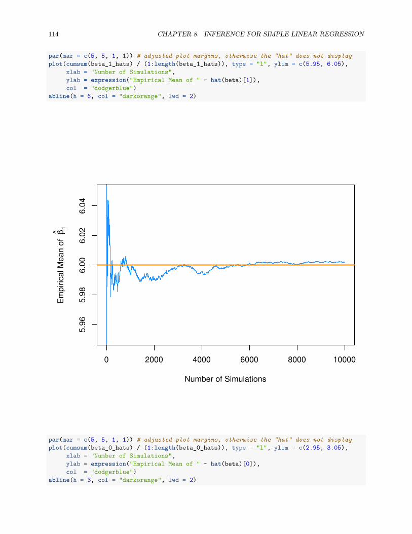
114 CHAPTER 8. INFERENCE FOR SIMPLE LINEAR REGRESSION
par(mar = c(5, 5, 1, 1)) # adjusted plot margins, otherwise the "hat" does not displayplot(cumsum(beta_1_hats) / (1:length(beta_1_hats)), type = "l", ylim = c(5.95, 6.05),
xlab = "Number of Simulations",ylab = expression("Empirical Mean of " ~ hat(beta)[1]),col = "dodgerblue")
abline(h = 6, col = "darkorange", lwd = 2)
0 2000 4000 6000 8000 10000
5.96
5.98
6.00
6.02
6.04
Number of Simulations
Em
piric
al M
ean
of β
1
par(mar = c(5, 5, 1, 1)) # adjusted plot margins, otherwise the "hat" does not displayplot(cumsum(beta_0_hats) / (1:length(beta_0_hats)), type = "l", ylim = c(2.95, 3.05),
xlab = "Number of Simulations",ylab = expression("Empirical Mean of " ~ hat(beta)[0]),col = "dodgerblue")
abline(h = 3, col = "darkorange", lwd = 2)
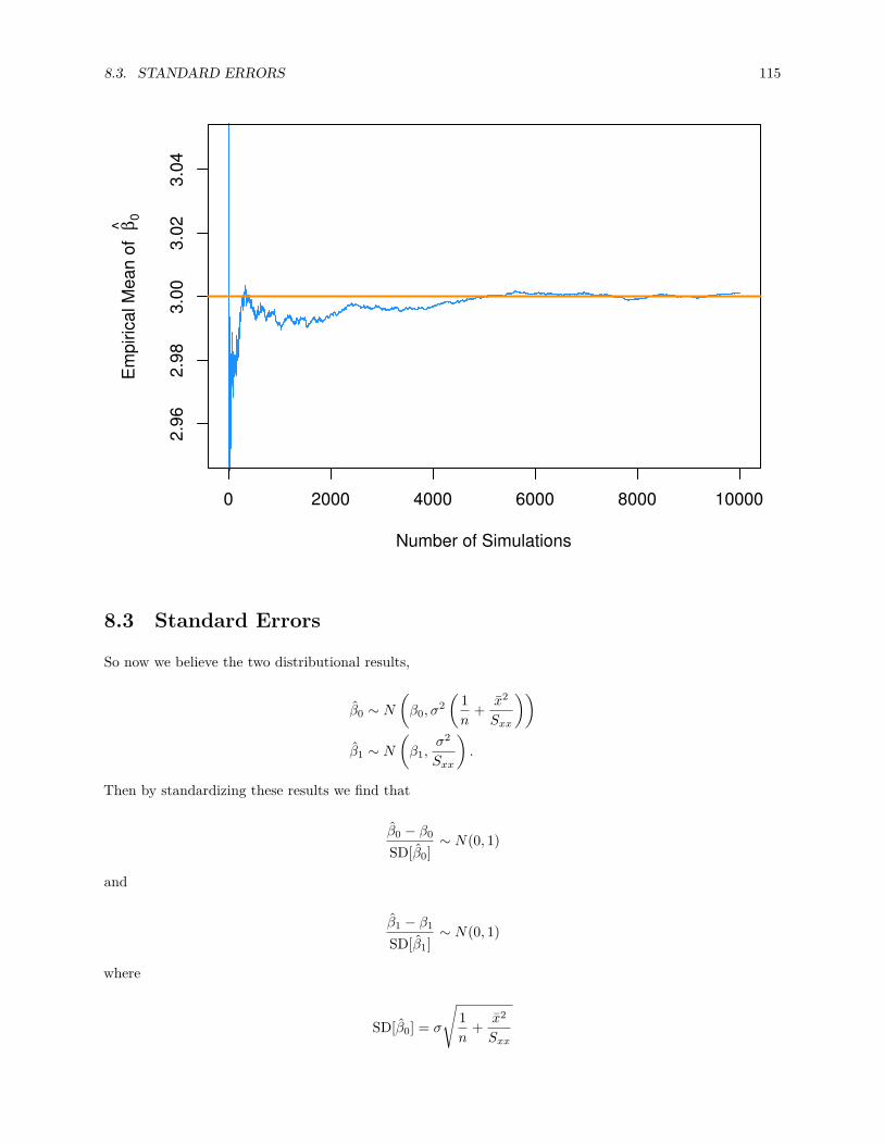
8.3. STANDARD ERRORS 115
0 2000 4000 6000 8000 10000
2.96
2.98
3.00
3.02
3.04
Number of Simulations
Em
piric
al M
ean
of β
0
8.3 Standard Errors
So now we believe the two distributional results,
β0 ∼ N
(β0, σ2
(1n
+ x2
Sxx
))β1 ∼ N
(β1,
σ2
Sxx
).
Then by standardizing these results we find that
β0 − β0
SD[β0]∼ N(0, 1)
and
β1 − β1
SD[β1]∼ N(0, 1)
where
SD[β0] = σ
√1n
+ x2
Sxx

116 CHAPTER 8. INFERENCE FOR SIMPLE LINEAR REGRESSION
and
SD[β1] = σ√Sxx
.
Since we don’t know σ in practice, we will have to estimate it using se, which we plug into our existingexpression for the standard deviations of our estimates.
These two new expressions are called standard errors which are the estimated standard deviations of thesampling distributions.
SE[β0] = se
√1n
+ x2
Sxx
SE[β1] = se√Sxx
Now if we divide by the standard error, instead of the standard deviation, we obtain the following resultswhich will allow us to make confidence intervals and perform hypothesis testing.
β0 − β0
SE[β0]∼ tn−2
β1 − β1
SE[β1]∼ tn−2
To see this, first note that,
RSSσ2 = (n − 2)s2
e
σ2 ∼ χ2n−2.
Also recall that a random variable T defined as,
T = Z√χ2
d
d
follows a t distribution with d degrees of freedom, where χ2d is a χ2 random variable with d degrees of freedom.
We write,
T ∼ td
to say that the random variable T follows a t distribution with d degrees of freedom.
Then we use the classic trick of “multiply by 1” and some rearranging to arrive at

8.3. STANDARD ERRORS 117
β1 − β1
SE[β1]= β1 − β1
se/√
Sxx
= β1 − β1
se/√
Sxx
· σ/√
Sxx
σ/√
Sxx
= β1 − β1
σ/√
Sxx
· σ/√
Sxx
se/√
Sxx
= β1 − β1
σ/√
Sxx
/√s2
e
σ2
= β1 − β1
SD[β1]
/√ (n−2)s2e
σ2
n − 2∼ Z√
χ2n−2
n−2
∼ tn−2
where Z ∼ N(0, 1).
Recall that a t distribution is similar to a standard normal, but with heavier tails. As the degrees of freedomincreases, the t distribution becomes more and more like a standard normal. Below we plot a standardnormal distribution as well as two examples of a t distribution with different degrees of freedom. Notice howthe t distribution with the larger degrees of freedom is more similar to the standard normal curve.
# define grid of x valuesx = seq(-4, 4, length = 100)
# plot curve for standard normalplot(x, dnorm(x), type = "l", lty = 1, lwd = 2,
xlab = "x", ylab = "Density", main = "Normal vs t Distributions")# add curves for t distributionslines(x, dt(x, df = 1), lty = 3, lwd = 2, col = "darkorange")lines(x, dt(x, df = 10), lty = 2, lwd = 2, col = "dodgerblue")
# add legendlegend("topright", title = "Distributions",
legend = c("t, df = 1", "t, df = 10", "Standard Normal"),lwd = 2, lty=c(3, 2, 1), col = c("darkorange", "dodgerblue", "black"))
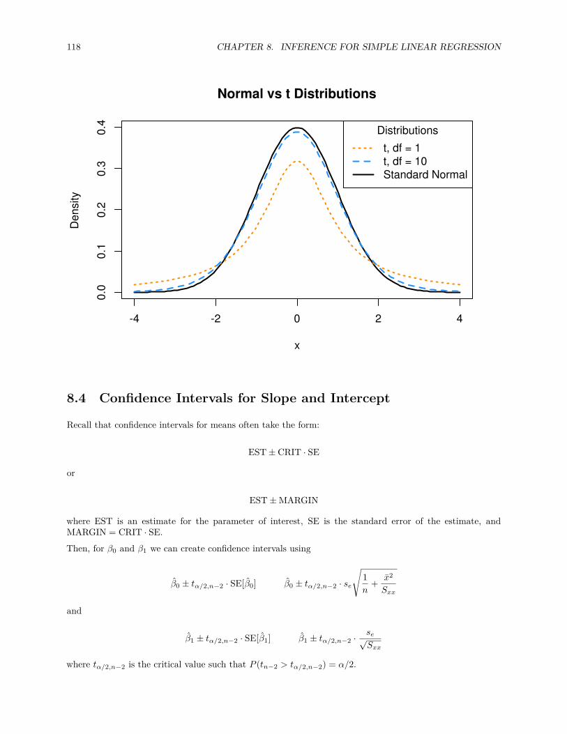
118 CHAPTER 8. INFERENCE FOR SIMPLE LINEAR REGRESSION
-4 -2 0 2 4
0.0
0.1
0.2
0.3
0.4
Normal vs t Distributions
x
Den
sity
Distributions
t, df = 1t, df = 10Standard Normal
8.4 Confidence Intervals for Slope and Intercept
Recall that confidence intervals for means often take the form:
EST ± CRIT · SE
or
EST ± MARGIN
where EST is an estimate for the parameter of interest, SE is the standard error of the estimate, andMARGIN = CRIT · SE.Then, for β0 and β1 we can create confidence intervals using
β0 ± tα/2,n−2 · SE[β0] β0 ± tα/2,n−2 · se
√1n
+ x2
Sxx
and
β1 ± tα/2,n−2 · SE[β1] β1 ± tα/2,n−2 · se√Sxx
where tα/2,n−2 is the critical value such that P (tn−2 > tα/2,n−2) = α/2.

8.5. HYPOTHESIS TESTS 119
8.5 Hypothesis Tests
“We may speak of this hypothesis as the ‘null hypothesis’, and it should be noted that the nullhypothesis is never proved or established, but is possibly disproved, in the course of experimen-tation.”
— Ronald Aylmer Fisher
Recall that a test statistic (TS) for testing means often take the form:
TS = EST − HYPSE
where EST is an estimate for the parameter of interest, HYP is a hypothesized value of the parameter, andSE is the standard error of the estimate.
So, to test
H0 : β0 = β00 vs H1 : β0 = β00
we use the test statistic
t = β0 − β00
SE[β0]= β0 − β00
se
√1n + x2
Sxx
which, under the null hypothesis, follows a t distribution with n−2 degrees of freedom. We use β00 to denotethe hypothesized value of β0.
Similarly, to test
H0 : β1 = β10 vs H1 : β1 = β10
we use the test statistic
t = β1 − β10
SE[β1]= β1 − β10
se/√
Sxx
which again, under the null hypothesis, follows a t distribution with n − 2 degrees of freedom. We now useβ10 to denote the hypothesized value of β1.
8.6 cars Example
We now return to the cars example from last chapter to illustrate these concepts. We first fit the modelusing lm() then use summary() to view the results in greater detail.
stop_dist_model = lm(dist ~ speed, data = cars)summary(stop_dist_model)
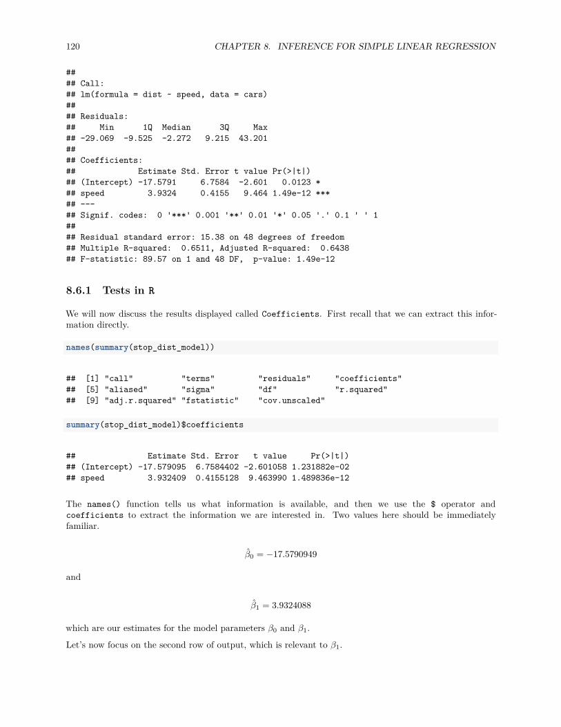
120 CHAPTER 8. INFERENCE FOR SIMPLE LINEAR REGRESSION
#### Call:## lm(formula = dist ~ speed, data = cars)#### Residuals:## Min 1Q Median 3Q Max## -29.069 -9.525 -2.272 9.215 43.201#### Coefficients:## Estimate Std. Error t value Pr(>|t|)## (Intercept) -17.5791 6.7584 -2.601 0.0123 *## speed 3.9324 0.4155 9.464 1.49e-12 ***## ---## Signif. codes: 0 '***' 0.001 '**' 0.01 '*' 0.05 '.' 0.1 ' ' 1#### Residual standard error: 15.38 on 48 degrees of freedom## Multiple R-squared: 0.6511, Adjusted R-squared: 0.6438## F-statistic: 89.57 on 1 and 48 DF, p-value: 1.49e-12
8.6.1 Tests in R
We will now discuss the results displayed called Coefficients. First recall that we can extract this infor-mation directly.
names(summary(stop_dist_model))
## [1] "call" "terms" "residuals" "coefficients"## [5] "aliased" "sigma" "df" "r.squared"## [9] "adj.r.squared" "fstatistic" "cov.unscaled"
summary(stop_dist_model)$coefficients
## Estimate Std. Error t value Pr(>|t|)## (Intercept) -17.579095 6.7584402 -2.601058 1.231882e-02## speed 3.932409 0.4155128 9.463990 1.489836e-12
The names() function tells us what information is available, and then we use the $ operator andcoefficients to extract the information we are interested in. Two values here should be immediatelyfamiliar.
β0 = −17.5790949
and
β1 = 3.9324088
which are our estimates for the model parameters β0 and β1.
Let’s now focus on the second row of output, which is relevant to β1.
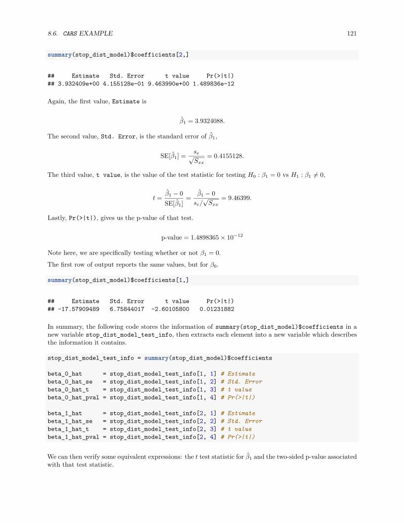
8.6. CARS EXAMPLE 121
summary(stop_dist_model)$coefficients[2,]
## Estimate Std. Error t value Pr(>|t|)## 3.932409e+00 4.155128e-01 9.463990e+00 1.489836e-12
Again, the first value, Estimate is
β1 = 3.9324088.
The second value, Std. Error, is the standard error of β1,
SE[β1] = se√Sxx
= 0.4155128.
The third value, t value, is the value of the test statistic for testing H0 : β1 = 0 vs H1 : β1 = 0,
t = β1 − 0SE[β1]
= β1 − 0se/
√Sxx
= 9.46399.
Lastly, Pr(>|t|), gives us the p-value of that test.
p-value = 1.4898365 × 10⁻¹²
Note here, we are specifically testing whether or not β1 = 0.
The first row of output reports the same values, but for β0.
summary(stop_dist_model)$coefficients[1,]
## Estimate Std. Error t value Pr(>|t|)## -17.57909489 6.75844017 -2.60105800 0.01231882
In summary, the following code stores the information of summary(stop_dist_model)$coefficients in anew variable stop_dist_model_test_info, then extracts each element into a new variable which describesthe information it contains.
stop_dist_model_test_info = summary(stop_dist_model)$coefficients
beta_0_hat = stop_dist_model_test_info[1, 1] # Estimatebeta_0_hat_se = stop_dist_model_test_info[1, 2] # Std. Errorbeta_0_hat_t = stop_dist_model_test_info[1, 3] # t valuebeta_0_hat_pval = stop_dist_model_test_info[1, 4] # Pr(>|t|)
beta_1_hat = stop_dist_model_test_info[2, 1] # Estimatebeta_1_hat_se = stop_dist_model_test_info[2, 2] # Std. Errorbeta_1_hat_t = stop_dist_model_test_info[2, 3] # t valuebeta_1_hat_pval = stop_dist_model_test_info[2, 4] # Pr(>|t|)
We can then verify some equivalent expressions: the t test statistic for β1 and the two-sided p-value associatedwith that test statistic.

122 CHAPTER 8. INFERENCE FOR SIMPLE LINEAR REGRESSION
(beta_1_hat - 0) / beta_1_hat_se
## [1] 9.46399
beta_1_hat_t
## [1] 9.46399
2 * pt(abs(beta_1_hat_t), df = length(resid(stop_dist_model)) - 2, lower.tail = FALSE)
## [1] 1.489836e-12
beta_1_hat_pval
## [1] 1.489836e-12
8.6.2 Significance of Regression, t-Test
We pause to discuss the significance of regression test. First, note that based on the above distributionalresults, we could test β0 and β1 against any particular value, and perform both one and two-sided tests.
However, one very specific test,
H0 : β1 = 0 vs H1 : β1 = 0
is used most often. Let’s think about this test in terms of the simple linear regression model,
Yi = β0 + β1xi + ϵi.
If we assume the null hypothesis is true, then β1 = 0 and we have the model,
Yi = β0 + ϵi.
In this model, the response does not depend on the predictor. So then we could think of this test in thefollowing way,
• Under H0 there is not a significant linear relationship between x and y.• Under H1 there is a significance linear relationship between x and y.
For the cars example,
• Under H0 there is not a significant linear relationship between speed and stopping distance.• Under H1 there is a significant linear relationship between speed and stopping distance.
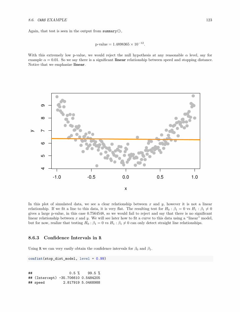
8.6. CARS EXAMPLE 123
Again, that test is seen in the output from summary(),
p-value = 1.4898365 × 10⁻¹².
With this extremely low p-value, we would reject the null hypothesis at any reasonable α level, say forexample α = 0.01. So we say there is a significant linear relationship between speed and stopping distance.Notice that we emphasize linear.
-1.0 -0.5 0.0 0.5 1.0
45
67
89
x
y
In this plot of simulated data, we see a clear relationship between x and y, however it is not a linearrelationship. If we fit a line to this data, it is very flat. The resulting test for H0 : β1 = 0 vs H1 : β1 = 0gives a large p-value, in this case 0.7564548, so we would fail to reject and say that there is no significantlinear relationship between x and y. We will see later how to fit a curve to this data using a “linear” model,but for now, realize that testing H0 : β1 = 0 vs H1 : β1 = 0 can only detect straight line relationships.
8.6.3 Confidence Intervals in R
Using R we can very easily obtain the confidence intervals for β0 and β1.
confint(stop_dist_model, level = 0.99)
## 0.5 % 99.5 %## (Intercept) -35.706610 0.5484205## speed 2.817919 5.0468988

124 CHAPTER 8. INFERENCE FOR SIMPLE LINEAR REGRESSION
This automatically calculates 99% confidence intervals for both β0 and β1, the first row for β0, the secondrow for β1.
For the cars example when interpreting these intervals, we say, we are 99% confident that for an increasein speed of 1 mile per hour, the average increase in stopping distance is between 2.8179187 and 5.0468988feet, which is the interval for β1.
Note that this 99% confidence interval does not contain the hypothesized value of 0. Since it does notcontain 0, it is equivalent to rejecting the test of H0 : β1 = 0 vs H1 : β1 = 0 at α = 0.01, which we had seenpreviously.
You should be somewhat suspicious of the confidence interval for β0, as it covers negative values, whichcorrespond to negative stopping distances. Technically the interpretation would be that we are 99% confidentthat the average stopping distance of a car traveling 0 miles per hour is between -35.7066103 and 0.5484205feet, but we don’t really believe that, since we are actually certain that it would be non-negative.
Note, we can extract specific values from this output a number of ways. This code is not run, and instead,you should check how it relates to the output of the code above.
confint(stop_dist_model, level = 0.99)[1,]confint(stop_dist_model, level = 0.99)[1, 1]confint(stop_dist_model, level = 0.99)[1, 2]confint(stop_dist_model, parm = "(Intercept)", level = 0.99)confint(stop_dist_model, level = 0.99)[2,]confint(stop_dist_model, level = 0.99)[2, 1]confint(stop_dist_model, level = 0.99)[2, 2]confint(stop_dist_model, parm = "speed", level = 0.99)
We can also verify that calculations that R is performing for the β1 interval.
# store estimatebeta_1_hat = coef(stop_dist_model)[2]
# store standard errorbeta_1_hat_se = summary(stop_dist_model)$coefficients[2, 2]
# calculate critical value for two-sided 99% CIcrit = qt(0.995, df = length(resid(stop_dist_model)) - 2)
# est - margin, est + marginc(beta_1_hat - crit * beta_1_hat_se, beta_1_hat + crit * beta_1_hat_se)
## speed speed## 2.817919 5.046899
8.7 Confidence Interval for Mean Response
In addition to confidence intervals for β0 and β1, there are two other common interval estimates used withregression. The first is called a confidence interval for the mean response. Often, we would like aninterval estimate for the mean, E[Y | X = x] for a particular value of x.
In this situation we use y(x) as our estimate of E[Y | X = x]. We modify our notation slightly to make itclear that the the predicted value is a function of the x value.

8.7. CONFIDENCE INTERVAL FOR MEAN RESPONSE 125
y(x) = β0 + β1x
Recall that,
E[Y | X = x] = β0 + β1x.
Thus, y(x) is a good estimate since it is unbiased:
E[y(x)] = β0 + β1x.
We could then derive,
Var[y(x)] = σ2(
1n
+ (x − x)2
Sxx
).
Like the other estimates we have seen, y(x) also follows a normal distribution. Since β0 and β1 are linearcombinations of normal random variables, y(x) is as well.
y(x) ∼ N
(β0 + β1x, σ2
(1n
+ (x − x)2
Sxx
))
And lastly, since we need to estimate this variance, we arrive at the standard error of our estimate,
SE[y(x)] = se
√1n
+ (x − x)2
Sxx.
We can then use this to find the confidence interval for the mean response,
y(x) ± tα/2,n−2 · se
√1n
+ (x − x)2
Sxx
To find confidence intervals for the mean response using R, we use the predict() function. We give thefunction our fitted model as well as new data, stored as a data frame. (This is important, so that R knows thename of the predictor variable.) Here, we are finding the confidence interval for the mean stopping distancewhen a car is travelling 5 miles per hour and when a car is travelling 21 miles per hour.
new_speeds = data.frame(speed = c(5, 21))predict(stop_dist_model, newdata = new_speeds,
interval = c("confidence"), level = 0.99)
## fit lwr upr## 1 2.082949 -10.89309 15.05898## 2 65.001489 56.45836 73.54462
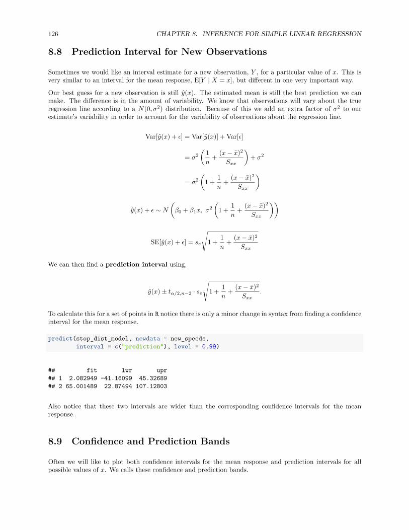
126 CHAPTER 8. INFERENCE FOR SIMPLE LINEAR REGRESSION
8.8 Prediction Interval for New Observations
Sometimes we would like an interval estimate for a new observation, Y , for a particular value of x. This isvery similar to an interval for the mean response, E[Y | X = x], but different in one very important way.
Our best guess for a new observation is still y(x). The estimated mean is still the best prediction we canmake. The difference is in the amount of variability. We know that observations will vary about the trueregression line according to a N(0, σ2) distribution. Because of this we add an extra factor of σ2 to ourestimate’s variability in order to account for the variability of observations about the regression line.
Var[y(x) + ϵ] = Var[y(x)] + Var[ϵ]
= σ2(
1n
+ (x − x)2
Sxx
)+ σ2
= σ2(
1 + 1n
+ (x − x)2
Sxx
)
y(x) + ϵ ∼ N
(β0 + β1x, σ2
(1 + 1
n+ (x − x)2
Sxx
))
SE[y(x) + ϵ] = se
√1 + 1
n+ (x − x)2
Sxx
We can then find a prediction interval using,
y(x) ± tα/2,n−2 · se
√1 + 1
n+ (x − x)2
Sxx.
To calculate this for a set of points in R notice there is only a minor change in syntax from finding a confidenceinterval for the mean response.
predict(stop_dist_model, newdata = new_speeds,interval = c("prediction"), level = 0.99)
## fit lwr upr## 1 2.082949 -41.16099 45.32689## 2 65.001489 22.87494 107.12803
Also notice that these two intervals are wider than the corresponding confidence intervals for the meanresponse.
8.9 Confidence and Prediction Bands
Often we will like to plot both confidence intervals for the mean response and prediction intervals for allpossible values of x. We calls these confidence and prediction bands.

8.9. CONFIDENCE AND PREDICTION BANDS 127
speed_grid = seq(min(cars$speed), max(cars$speed), by = 0.01)dist_ci_band = predict(stop_dist_model,
newdata = data.frame(speed = speed_grid),interval = "confidence", level = 0.99)
dist_pi_band = predict(stop_dist_model,newdata = data.frame(speed = speed_grid),interval = "prediction", level = 0.99)
plot(dist ~ speed, data = cars,xlab = "Speed (in Miles Per Hour)",ylab = "Stopping Distance (in Feet)",main = "Stopping Distance vs Speed",pch = 20,cex = 2,col = "grey",ylim = c(min(dist_pi_band), max(dist_pi_band)))
abline(stop_dist_model, lwd = 5, col = "darkorange")
lines(speed_grid, dist_ci_band[,"lwr"], col = "dodgerblue", lwd = 3, lty = 2)lines(speed_grid, dist_ci_band[,"upr"], col = "dodgerblue", lwd = 3, lty = 2)lines(speed_grid, dist_pi_band[,"lwr"], col = "dodgerblue", lwd = 3, lty = 3)lines(speed_grid, dist_pi_band[,"upr"], col = "dodgerblue", lwd = 3, lty = 3)points(mean(cars$speed), mean(cars$dist), pch = "+", cex = 3)
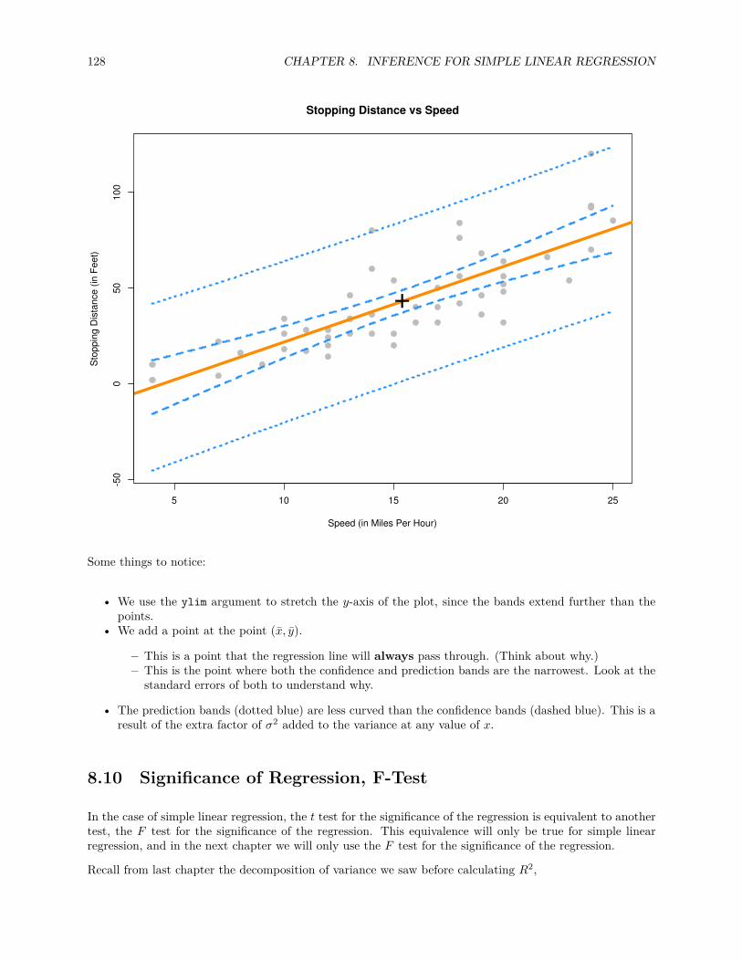
128 CHAPTER 8. INFERENCE FOR SIMPLE LINEAR REGRESSION
5 10 15 20 25
-50
050
100
Stopping Distance vs Speed
Speed (in Miles Per Hour)
Sto
ppin
g D
ista
nce
(in F
eet)
+
Some things to notice:
• We use the ylim argument to stretch the y-axis of the plot, since the bands extend further than thepoints.
• We add a point at the point (x, y).
– This is a point that the regression line will always pass through. (Think about why.)– This is the point where both the confidence and prediction bands are the narrowest. Look at the
standard errors of both to understand why.
• The prediction bands (dotted blue) are less curved than the confidence bands (dashed blue). This is aresult of the extra factor of σ2 added to the variance at any value of x.
8.10 Significance of Regression, F-Test
In the case of simple linear regression, the t test for the significance of the regression is equivalent to anothertest, the F test for the significance of the regression. This equivalence will only be true for simple linearregression, and in the next chapter we will only use the F test for the significance of the regression.
Recall from last chapter the decomposition of variance we saw before calculating R2,
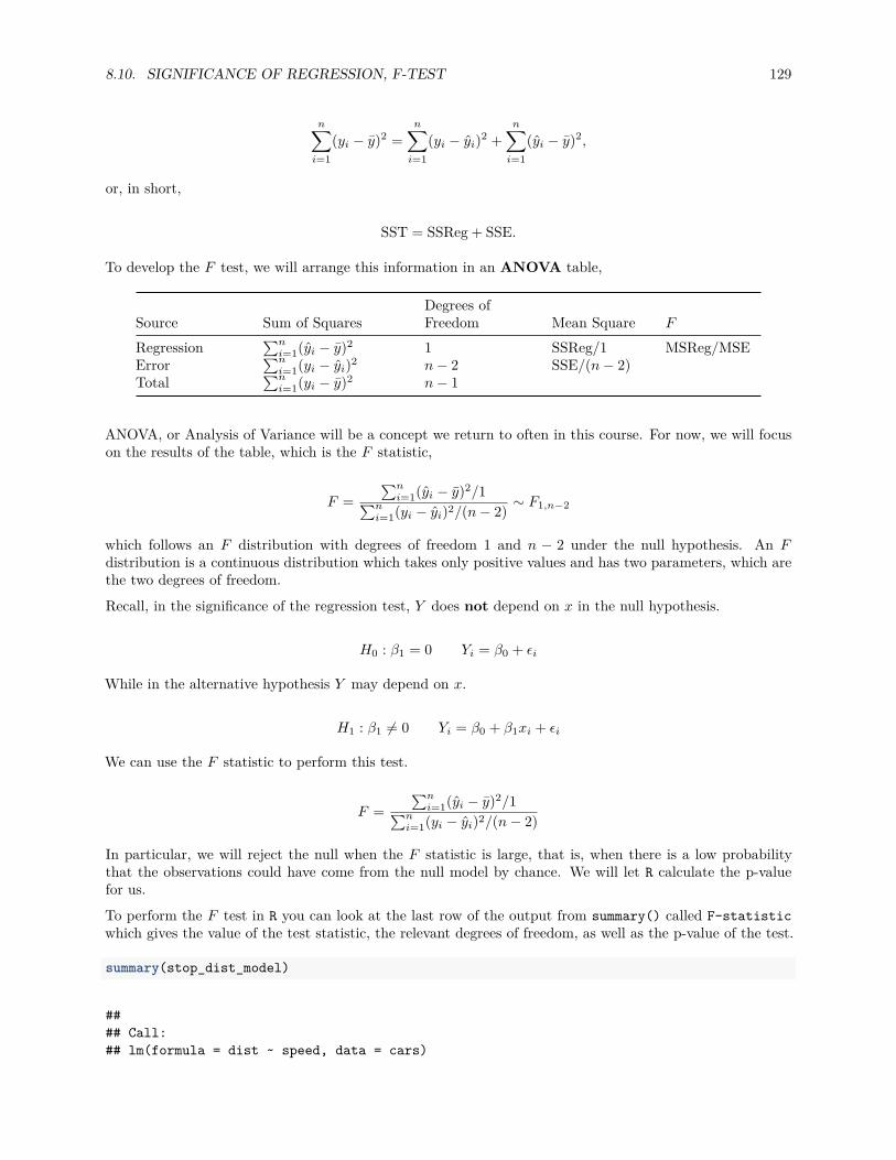
8.10. SIGNIFICANCE OF REGRESSION, F-TEST 129
n∑i=1
(yi − y)2 =n∑
i=1(yi − yi)2 +
n∑i=1
(yi − y)2,
or, in short,
SST = SSReg + SSE.
To develop the F test, we will arrange this information in an ANOVA table,
Source Sum of SquaresDegrees ofFreedom Mean Square F
Regression∑n
i=1(yi − y)2 1 SSReg/1 MSReg/MSEError
∑ni=1(yi − yi)2 n − 2 SSE/(n − 2)
Total∑n
i=1(yi − y)2 n − 1
ANOVA, or Analysis of Variance will be a concept we return to often in this course. For now, we will focuson the results of the table, which is the F statistic,
F =∑n
i=1(yi − y)2/1∑ni=1(yi − yi)2/(n − 2)
∼ F1,n−2
which follows an F distribution with degrees of freedom 1 and n − 2 under the null hypothesis. An Fdistribution is a continuous distribution which takes only positive values and has two parameters, which arethe two degrees of freedom.
Recall, in the significance of the regression test, Y does not depend on x in the null hypothesis.
H0 : β1 = 0 Yi = β0 + ϵi
While in the alternative hypothesis Y may depend on x.
H1 : β1 = 0 Yi = β0 + β1xi + ϵi
We can use the F statistic to perform this test.
F =∑n
i=1(yi − y)2/1∑ni=1(yi − yi)2/(n − 2)
In particular, we will reject the null when the F statistic is large, that is, when there is a low probabilitythat the observations could have come from the null model by chance. We will let R calculate the p-valuefor us.
To perform the F test in R you can look at the last row of the output from summary() called F-statisticwhich gives the value of the test statistic, the relevant degrees of freedom, as well as the p-value of the test.
summary(stop_dist_model)
#### Call:## lm(formula = dist ~ speed, data = cars)

130 CHAPTER 8. INFERENCE FOR SIMPLE LINEAR REGRESSION
#### Residuals:## Min 1Q Median 3Q Max## -29.069 -9.525 -2.272 9.215 43.201#### Coefficients:## Estimate Std. Error t value Pr(>|t|)## (Intercept) -17.5791 6.7584 -2.601 0.0123 *## speed 3.9324 0.4155 9.464 1.49e-12 ***## ---## Signif. codes: 0 '***' 0.001 '**' 0.01 '*' 0.05 '.' 0.1 ' ' 1#### Residual standard error: 15.38 on 48 degrees of freedom## Multiple R-squared: 0.6511, Adjusted R-squared: 0.6438## F-statistic: 89.57 on 1 and 48 DF, p-value: 1.49e-12
Additionally, you can use the anova() function to display the information in an ANOVA table.
anova(stop_dist_model)
## Analysis of Variance Table#### Response: dist## Df Sum Sq Mean Sq F value Pr(>F)## speed 1 21186 21185.5 89.567 1.49e-12 ***## Residuals 48 11354 236.5## ---## Signif. codes: 0 '***' 0.001 '**' 0.01 '*' 0.05 '.' 0.1 ' ' 1
This also gives a p-value for the test. You should notice that the p-value from the t test was the same. Youmight also notice that the value of the test statistic for the t test, 9.46399, can be squared to obtain thevalue of the F statistic, 89.5671065.Note that there is another equivalent way to do this in R, which we will return to often to compare twomodels.
anova(lm(dist ~ 1, data = cars), lm(dist ~ speed, data = cars))
## Analysis of Variance Table#### Model 1: dist ~ 1## Model 2: dist ~ speed## Res.Df RSS Df Sum of Sq F Pr(>F)## 1 49 32539## 2 48 11354 1 21186 89.567 1.49e-12 ***## ---## Signif. codes: 0 '***' 0.001 '**' 0.01 '*' 0.05 '.' 0.1 ' ' 1
The model statement lm(dist ~ 1, data = cars) applies the model Yi = β0 + ϵi to the cars data. Notethat y = y when Yi = β0 + ϵi.The model statement lm(dist ~ speed, data = cars) applies the model Yi = β0 + β1xi + ϵi.We can then think of this usage of anova() as directly comparing the two models. (Notice we get the samep-value again.)
Chapter 9
Multiple Linear Regression
“Life is really simple, but we insist on making it complicated.”— Confucius
After reading this chapter you will be able to:
• Construct and interpret linear regression models with more than one predictor.• Understand how regression models are derived using matrices.• Create interval estimates and perform hypothesis tests for multiple regression parameters.• Formulate and interpret interval estimates for the mean response under various conditions.• Compare nested models using an ANOVA F-Test.
The last two chapters we saw how to fit a model that assumed a linear relationship between a responsevariable and a single predictor variable. Specifically, we defined the simple linear regression model,
Yi = β0 + β1xi + ϵi
where ϵi ∼ N(0, σ2).
However, it is rarely the case that a dataset will have a single predictor variable. It is also rarely the casethat a response variable will only depend on a single variable. So in this chapter, we will extend our currentlinear model to allow a response to depend on multiple predictors.
# read the data from the webautompg = read.table("http://archive.ics.uci.edu/ml/machine-learning-databases/auto-mpg/auto-mpg.data",quote = "\"",comment.char = "",stringsAsFactors = FALSE)
# give the dataframe headerscolnames(autompg) = c("mpg", "cyl", "disp", "hp", "wt", "acc", "year", "origin", "name")# remove missing data, which is stored as "?"autompg = subset(autompg, autompg$hp != "?")# remove the plymouth reliant, as it causes some issuesautompg = subset(autompg, autompg$name != "plymouth reliant")# give the dataset row names, based on the engine, year and namerownames(autompg) = paste(autompg$cyl, "cylinder", autompg$year, autompg$name)
131

132 CHAPTER 9. MULTIPLE LINEAR REGRESSION
# remove the variable for name, as well as originautompg = subset(autompg, select = c("mpg", "cyl", "disp", "hp", "wt", "acc", "year"))# change horsepower from character to numericautompg$hp = as.numeric(autompg$hp)# check final structure of datastr(autompg)
## 'data.frame': 390 obs. of 7 variables:## $ mpg : num 18 15 18 16 17 15 14 14 14 15 ...## $ cyl : int 8 8 8 8 8 8 8 8 8 8 ...## $ disp: num 307 350 318 304 302 429 454 440 455 390 ...## $ hp : num 130 165 150 150 140 198 220 215 225 190 ...## $ wt : num 3504 3693 3436 3433 3449 ...## $ acc : num 12 11.5 11 12 10.5 10 9 8.5 10 8.5 ...## $ year: int 70 70 70 70 70 70 70 70 70 70 ...
We will once again discuss a dataset with information about cars. This dataset, which can be found at theUCI Machine Learning Repository contains a response variable mpg which stores the city fuel efficiency ofcars, as well as several predictor variables for the attributes of the vehicles. We load the data, and performsome basic tidying before moving on to analysis.
For now we will focus on using two variables, wt and year, as predictor variables. That is, we would like tomodel the fuel efficiency (mpg) of a car as a function of its weight (wt) and model year (year). To do so, wewill define the following linear model,
Yi = β0 + β1xi1 + β2xi2 + ϵi, i = 1, 2, . . . , n
where ϵi ∼ N(0, σ2). In this notation we will define:
• xi1 as the weight (wt) of the ith car.• xi2 as the model year (year) of the ith car.
The picture below will visualize what we would like to accomplish. The data points (xi1, xi2, yi) now exist in3-dimensional space, so instead of fitting a line to the data, we will fit a plane. (We’ll soon move to higherdimensions, so this will be the last example that is easy to visualize and think about this way.)

133
wt
20003000
4000
5000
year
70
72
74
76
788082m
pg
0
10
20
30
40
0
10
20
30
40
How do we find such a plane? Well, we would like a plane that is as close as possible to the data points.That is, we would like it to minimize the errors it is making. How will we define these errors? Squareddistance of course! So, we would like to minimize
f(β0, β1, β2) =n∑
i=1(yi − (β0 + β1xi1 + β2xi2))2
with respect to β0, β1, and β2. How do we do so? It is another straightforward multivariate calculus problem.All we have done is add an extra variable since we did this last time. So again, we take a derivative withrespect to each of β0, β1, and β2 and set them equal to zero, then solve the resulting system of equations.That is,

134 CHAPTER 9. MULTIPLE LINEAR REGRESSION
∂f
∂β0= 0
∂f
∂β1= 0
∂f
∂β2= 0
After doing so, we will once again obtain the normal equations.
nβ0 + β1
n∑i=1
xi1 + β2
n∑i=1
xi2 =n∑
i=1yi
β0
n∑i=1
xi1 + β1
n∑i=1
x2i1 + β2
n∑i=1
xi1xi2 =n∑
i=1xi1yi
β0
n∑i=1
xi2 + β1
n∑i=1
xi1xi2 + β2
n∑i=1
x2i2 =
n∑i=1
xi2yi
We now have three equations and three variables, which we could solve, or we could simply let R solve forus.
mpg_model = lm(mpg ~ wt + year, data = autompg)coef(mpg_model)
## (Intercept) wt year## -14.637641945 -0.006634876 0.761401955
y = −14.6376419 + −0.0066349x1 + 0.761402x2
Here we have once again fit our model using lm(), however we have introduced a new syntactical element.The formula mpg ~ wt + year now reads: “model the response variable mpg as a linear function of wt andyear”. That is, it will estimate an intercept, as well as slope coefficients for wt and year. We then extractthese as we have done before using coef().In the multiple linear regression setting, some of the interpretations of the coefficients change slightly.Here, β0 = −14.6376419 is our estimate for β0, the mean miles per gallon for a car that weighs 0 poundsand was built in 1900. We see our estimate here is negative, which is a physical impossibility. However, thisisn’t unexpected, as we shouldn’t expect our model to be accurate for cars from 1900 which weigh 0 pounds.(Because they never existed!) This isn’t much of a change from SLR. That is, β0 is still simply the meanwhen all of the predictors are 0.The interpretation of the coefficients in front of our predictors are slightly different than before. For exampleβ1 = −0.0066349 is our estimate for β1, the average change in miles per gallon for an increase in weight (x1)of one-pound for a car of a certain model year, that is, for a fixed value of x2. Note that this coefficientis actually the same for any given value of x2. Later, we will look at models that allow for a different changein mean response for different values of x2. Also note that this estimate is negative, which we would expectsince, in general, fuel efficiency decreases for larger vehicles. Recall that in the multiple linear regressionsetting, this interpretation is dependent on a fixed value for x2, that is, “for a car of a certain model year.” Itis possible that the indirect relationship between fuel efficiency and weight does not hold when an additionalfactor, say year, is included, and thus we could have the sign of our coefficient flipped.Lastly, β2 = 0.761402 is our estimate for β2, the average change in miles per gallon for a one-year increasein model year (x2) for a car of a certain weight, that is, for a fixed value of x1. It is not surprising that the
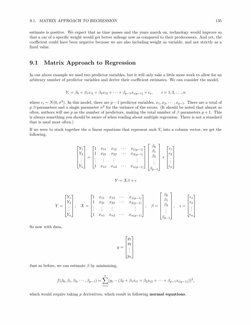
9.1. MATRIX APPROACH TO REGRESSION 135
estimate is positive. We expect that as time passes and the years march on, technology would improve sothat a car of a specific weight would get better mileage now as compared to their predecessors. And yet, thecoefficient could have been negative because we are also including weight as variable, and not strictly as afixed value.
9.1 Matrix Approach to Regression
In our above example we used two predictor variables, but it will only take a little more work to allow for anarbitrary number of predictor variables and derive their coefficient estimates. We can consider the model,
Yi = β0 + β1xi1 + β2xi2 + · · · + βp−1xi(p−1) + ϵi, i = 1, 2, . . . , n
where ϵi ∼ N(0, σ2). In this model, there are p − 1 predictor variables, x1, x2, · · · , xp−1. There are a total ofp β-parameters and a single parameter σ2 for the variance of the errors. (It should be noted that almost asoften, authors will use p as the number of predictors, making the total number of β parameters p + 1. Thisis always something you should be aware of when reading about multiple regression. There is not a standardthat is used most often.)
If we were to stack together the n linear equations that represent each Yi into a column vector, we get thefollowing.
Y1Y2...
Yn
=
1 x11 x12 · · · x1(p−1)1 x21 x22 · · · x2(p−1)...
......
...1 xn1 xn2 · · · xn(p−1)
β0β1β2...
βp−1
+
ϵ1ϵ2...
ϵn
Y = Xβ + ϵ
Y =
Y1Y2...
Yn
, X =
1 x11 x12 · · · x1(p−1)1 x21 x22 · · · x2(p−1)...
......
...1 xn1 xn2 · · · xn(p−1)
, β =
β0β1β2...
βp−1
, ϵ =
ϵ1ϵ2...
ϵn
So now with data,
y =
y1y2...
yn
Just as before, we can estimate β by minimizing,
f(β0, β1, β2, · · · , βp−1) =n∑
i=1(yi − (β0 + β1xi1 + β2xi2 + · · · + βp−1xi(p−1)))2,
which would require taking p derivatives, which result in following normal equations.
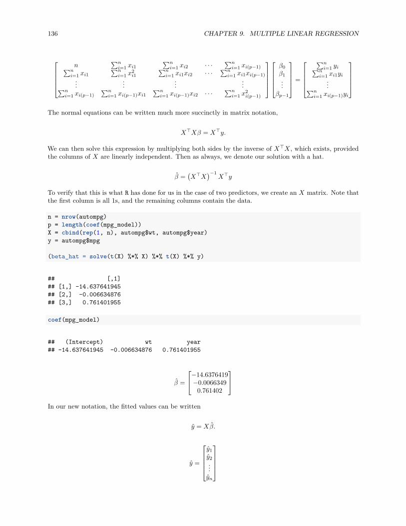
136 CHAPTER 9. MULTIPLE LINEAR REGRESSION
n
∑ni=1 xi1
∑ni=1 xi2 · · ·
∑ni=1 xi(p−1)∑n
i=1 xi1∑n
i=1 x2i1
∑ni=1 xi1xi2 · · ·
∑ni=1 xi1xi(p−1)
......
......∑n
i=1 xi(p−1)∑n
i=1 xi(p−1)xi1∑n
i=1 xi(p−1)xi2 · · ·∑n
i=1 x2i(p−1)
β0β1...
βp−1
=
∑n
i=1 yi∑ni=1 xi1yi
...∑ni=1 xi(p−1)yi
The normal equations can be written much more succinctly in matrix notation,
X⊤Xβ = X⊤y.
We can then solve this expression by multiplying both sides by the inverse of X⊤X, which exists, providedthe columns of X are linearly independent. Then as always, we denote our solution with a hat.
β =(X⊤X
)−1X⊤y
To verify that this is what R has done for us in the case of two predictors, we create an X matrix. Note thatthe first column is all 1s, and the remaining columns contain the data.
n = nrow(autompg)p = length(coef(mpg_model))X = cbind(rep(1, n), autompg$wt, autompg$year)y = autompg$mpg
(beta_hat = solve(t(X) %*% X) %*% t(X) %*% y)
## [,1]## [1,] -14.637641945## [2,] -0.006634876## [3,] 0.761401955
coef(mpg_model)
## (Intercept) wt year## -14.637641945 -0.006634876 0.761401955
β =
−14.6376419−0.0066349
0.761402
In our new notation, the fitted values can be written
y = Xβ.
y =
y1y2...
yn

9.1. MATRIX APPROACH TO REGRESSION 137
Then, we can create a vector for the residual values,
e =
e1e2...
en
=
y1y2...
yn
−
y1y2...
yn
.
And lastly, we can update our estimate for σ2.
s2e =
∑ni=1(yi − yi)2
n − p= e⊤e
n − p
Recall, we like this estimate because it is unbiased, that is,
E[s2e] = σ2
Note that the change from the SLR estimate to now is in the denominator. Specifically we now divide byn − p instead of n − 2. Or actually, we should note that in the case of SLR, there are two β parameters andthus p = 2.
Also note that if we fit the model Yi = β + ϵi that y = y and p = 1 and s2e would become
s2e =
∑ni=1(yi − y)2
n − 1
which is likely the very first sample standard deviation you saw in a mathematical statistics class. The samereason for n − 1 in this case, that we estimated one parameter, so we lose one degree of freedom. Now, ingeneral, we are estimating p parameters, the β parameters, so we lose p degrees of freedom.
Also, recall that most often we will be interested in se, the residual standard error as R calls it,
se =
√∑ni=1(yi − yi)2
n − p.
In R, we could directly access se for a fitted model, as we have seen before.
summary(mpg_model)$sigma
## [1] 3.431367
And we can now verify that our math above is indeed calculating the same quantities.
y_hat = X %*% solve(t(X) %*% X) %*% t(X) %*% ye = y - y_hatsqrt(t(e) %*% e / (n - p))
## [,1]## [1,] 3.431367
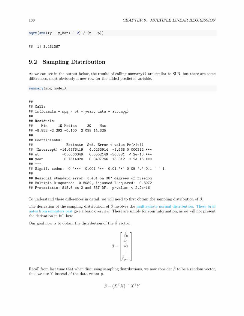
138 CHAPTER 9. MULTIPLE LINEAR REGRESSION
sqrt(sum((y - y_hat) ^ 2) / (n - p))
## [1] 3.431367
9.2 Sampling Distribution
As we can see in the output below, the results of calling summary() are similar to SLR, but there are somedifferences, most obviously a new row for the added predictor variable.
summary(mpg_model)
#### Call:## lm(formula = mpg ~ wt + year, data = autompg)#### Residuals:## Min 1Q Median 3Q Max## -8.852 -2.292 -0.100 2.039 14.325#### Coefficients:## Estimate Std. Error t value Pr(>|t|)## (Intercept) -14.6376419 4.0233914 -3.638 0.000312 ***## wt -0.0066349 0.0002149 -30.881 < 2e-16 ***## year 0.7614020 0.0497266 15.312 < 2e-16 ***## ---## Signif. codes: 0 '***' 0.001 '**' 0.01 '*' 0.05 '.' 0.1 ' ' 1#### Residual standard error: 3.431 on 387 degrees of freedom## Multiple R-squared: 0.8082, Adjusted R-squared: 0.8072## F-statistic: 815.6 on 2 and 387 DF, p-value: < 2.2e-16
To understand these differences in detail, we will need to first obtain the sampling distribution of β.
The derivation of the sampling distribution of β involves the multivariate normal distribution. These briefnotes from semesters past give a basic overview. These are simply for your information, as we will not presentthe derivation in full here.
Our goal now is to obtain the distribution of the β vector,
β =
β0β1β2...
βp−1
Recall from last time that when discussing sampling distributions, we now consider β to be a random vector,thus we use Y instead of the data vector y.
β =(X⊤X
)−1X⊤Y

9.2. SAMPLING DISTRIBUTION 139
Then it is a consequence of the multivariate normal distribution that,
β ∼ N(
β, σ2 (X⊤X)−1)
.
We then have
E[β] = β
and for any βj we have
E[βj ] = βj .
We also have
Var[β] = σ2 (X⊤X)−1
and for any βj we have
Var[βj ] = σ2Cjj
where
C =(X⊤X
)−1
and the elements of C are denoted
C =
C00 C01 C02 · · · C0(p−1)C10 C11 C12 · · · C1(p−1)C20 C21 C22 · · · C2(p−1)
......
......
C(p−1)0 C(p−1)1 C(p−1)2 · · · C(p−1)(p−1)
.
Essentially, the diagonal elements correspond to the β vector.
Then the standard error for the β vector is given by
SE[β] = se
√(X⊤X)−1
and for a particular βj
SE[βj ] = se
√Cjj .
Lastly, each of the βj follows a normal distribution,
βj ∼ N(βj , σ2Cjj
).
thus

140 CHAPTER 9. MULTIPLE LINEAR REGRESSION
βj − βj
se
√Cjj
∼ tn−p.
Now that we have the necessary distributional results, we can move on to perform tests and make intervalestimates.
9.2.1 Single Parameter Tests
The first test we will see is a test for a single βj .
H0 : βj = 0 vs H1 : βj = 0
Again, the test statistic takes the form
TS = EST − HYPSE .
In particular,
t = βj − βj
SE[βj ]= βj − 0
se
√Cjj
,
which, under the null hypothesis, follows a t distribution with n − p degrees of freedom.Recall our model for mpg,
Yi = β0 + β1xi1 + β2xi2 + ϵi, i = 1, 2, . . . , n
where ϵi ∼ N(0, σ2).
• xi1 as the weight (wt) of the ith car.• xi2 as the model year (year) of the ith car.
Then the test
H0 : β1 = 0 vs H1 : β1 = 0
can be found in the summary() output, in particular:
summary(mpg_model)$coef
## Estimate Std. Error t value Pr(>|t|)## (Intercept) -14.637641945 4.0233913563 -3.638135 3.118311e-04## wt -0.006634876 0.0002148504 -30.881372 1.850466e-106## year 0.761401955 0.0497265950 15.311765 1.036597e-41
The estimate (Estimate), standard error (Std. Error), test statistic (t value), and p-value (Pr(>|t|)) forthis test are displayed in the second row, labeled wt. Remember that the p-value given here is specificallyfor a two-sided test, where the hypothesized value is 0.Also note in this case, by hypothesizing that β1 = 0 the null and alternative essentially specify two differentmodels:
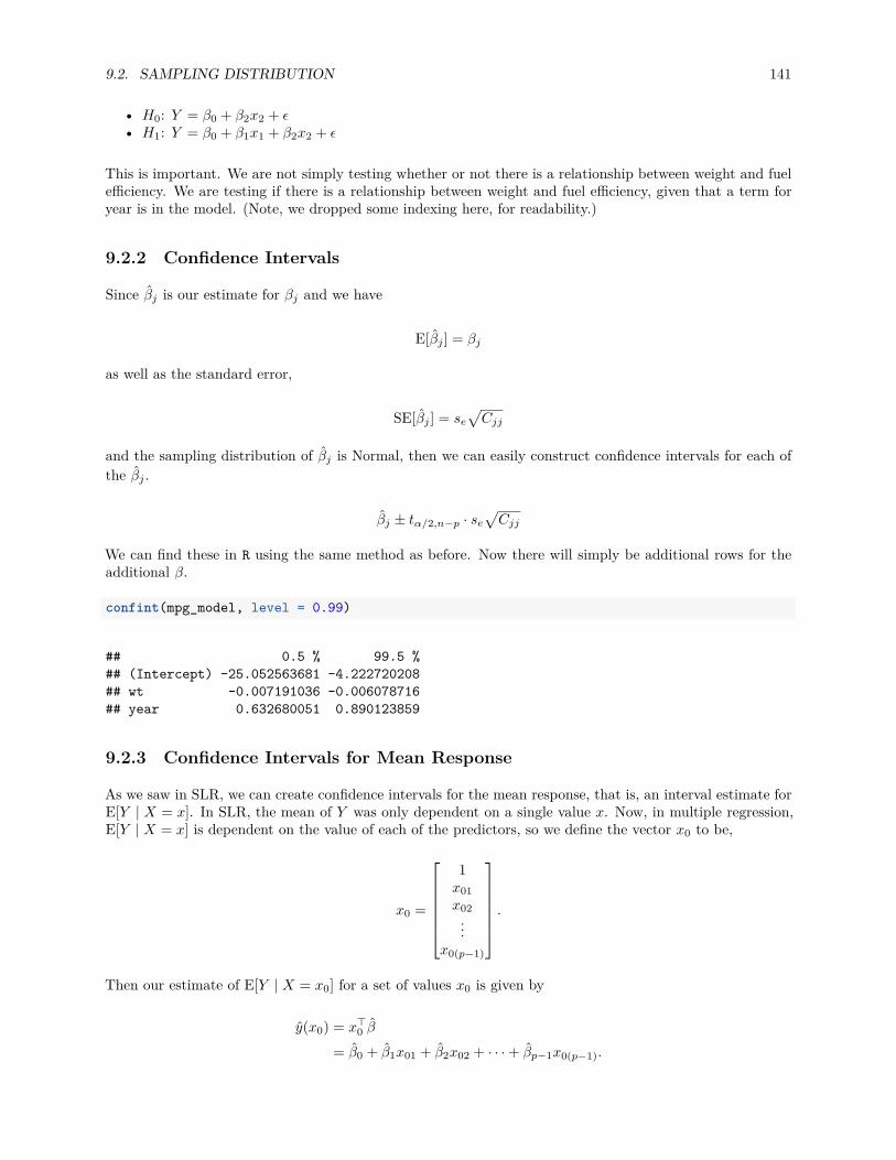
9.2. SAMPLING DISTRIBUTION 141
• H0: Y = β0 + β2x2 + ϵ• H1: Y = β0 + β1x1 + β2x2 + ϵ
This is important. We are not simply testing whether or not there is a relationship between weight and fuelefficiency. We are testing if there is a relationship between weight and fuel efficiency, given that a term foryear is in the model. (Note, we dropped some indexing here, for readability.)
9.2.2 Confidence Intervals
Since βj is our estimate for βj and we have
E[βj ] = βj
as well as the standard error,
SE[βj ] = se
√Cjj
and the sampling distribution of βj is Normal, then we can easily construct confidence intervals for each ofthe βj .
βj ± tα/2,n−p · se
√Cjj
We can find these in R using the same method as before. Now there will simply be additional rows for theadditional β.
confint(mpg_model, level = 0.99)
## 0.5 % 99.5 %## (Intercept) -25.052563681 -4.222720208## wt -0.007191036 -0.006078716## year 0.632680051 0.890123859
9.2.3 Confidence Intervals for Mean Response
As we saw in SLR, we can create confidence intervals for the mean response, that is, an interval estimate forE[Y | X = x]. In SLR, the mean of Y was only dependent on a single value x. Now, in multiple regression,E[Y | X = x] is dependent on the value of each of the predictors, so we define the vector x0 to be,
x0 =
1
x01x02
...x0(p−1)
.
Then our estimate of E[Y | X = x0] for a set of values x0 is given by
y(x0) = x⊤0 β
= β0 + β1x01 + β2x02 + · · · + βp−1x0(p−1).
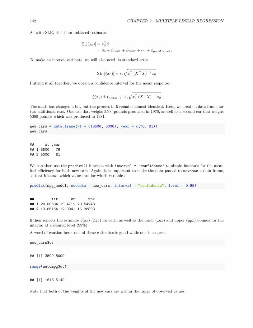
142 CHAPTER 9. MULTIPLE LINEAR REGRESSION
As with SLR, this is an unbiased estimate.
E[y(x0)] = x⊤0 β
= β0 + β1x01 + β2x02 + · · · + βp−1x0(p−1)
To make an interval estimate, we will also need its standard error.
SE[y(x0)] = se
√x⊤
0 (X⊤X)−1x0
Putting it all together, we obtain a confidence interval for the mean response.
y(x0) ± tα/2,n−p · se
√x⊤
0 (X⊤X)−1x0
The math has changed a bit, but the process in R remains almost identical. Here, we create a data frame fortwo additional cars. One car that weighs 3500 pounds produced in 1976, as well as a second car that weighs5000 pounds which was produced in 1981.
new_cars = data.frame(wt = c(3500, 5000), year = c(76, 81))new_cars
## wt year## 1 3500 76## 2 5000 81
We can then use the predict() function with interval = "confidence" to obtain intervals for the meanfuel efficiency for both new cars. Again, it is important to make the data passed to newdata a data frame,so that R knows which values are for which variables.
predict(mpg_model, newdata = new_cars, interval = "confidence", level = 0.99)
## fit lwr upr## 1 20.00684 19.4712 20.54248## 2 13.86154 12.3341 15.38898
R then reports the estimate y(x0) (fit) for each, as well as the lower (lwr) and upper (upr) bounds for theinterval at a desired level (99%).
A word of caution here: one of these estimates is good while one is suspect.
new_cars$wt
## [1] 3500 5000
range(autompg$wt)
## [1] 1613 5140
Note that both of the weights of the new cars are within the range of observed values.

9.2. SAMPLING DISTRIBUTION 143
new_cars$year
## [1] 76 81
range(autompg$year)
## [1] 70 82
As are the years of each of the new cars.
plot(year ~ wt, data = autompg, pch = 20, col = "dodgerblue", cex = 1.5)points(new_cars, col = "darkorange", cex = 3, pch = "X")
1500 2000 2500 3000 3500 4000 4500 5000
7072
7476
7880
82
wt
year X
X
However, we have to consider weight and year together now. And based on the above plot, one of the newcars is within the “blob” of observed values, while the other, the car from 1981 weighing 5000 pounds, isnoticeably outside of the observed values. This is a hidden extrapolation which you should be aware of whenusing multiple regression.
Shifting gears back to the new data pair that can be reasonably estimated, we do a quick verification of someof the mathematics in R.
x0 = c(1, 3500, 76)x0 %*% beta_hat

144 CHAPTER 9. MULTIPLE LINEAR REGRESSION
## [,1]## [1,] 20.00684
x0 =
1350076
β =
−14.6376419−0.0066349
0.761402
y(x0) = x⊤0 β =
[1 3500 76
] −14.6376419−0.0066349
0.761402
= 20.0068411
Also note that, using a particular value for x0, we can essentially extract certain βj values.
beta_hat
## [,1]## [1,] -14.637641945## [2,] -0.006634876## [3,] 0.761401955
x0 = c(0, 0, 1)x0 %*% beta_hat
## [,1]## [1,] 0.761402
With this in mind, confidence intervals for the individual βj are actually a special case of a confidence intervalfor mean response.
9.2.4 Prediction Intervals
As with SLR, creating prediction intervals involves one slight change to the standard error to account forthe fact that we are now considering an observation, instead of a mean.
Here we use y(x0) to estimate Y0, a new observation of Y at the predictor vector x0.
y(x0) = x⊤0 β
= β0 + β1x01 + β2x02 + · · · + βp−1x0(p−1)
E[y(x0)] = x⊤0 β
= β0 + β1x01 + β2x02 + · · · + βp−1x0(p−1)
As we did with SLR, we need to account for the additional variability of an observation about its mean.
SE[y(x0) + ϵ] = se
√1 + x⊤
0 (X⊤X)−1x0
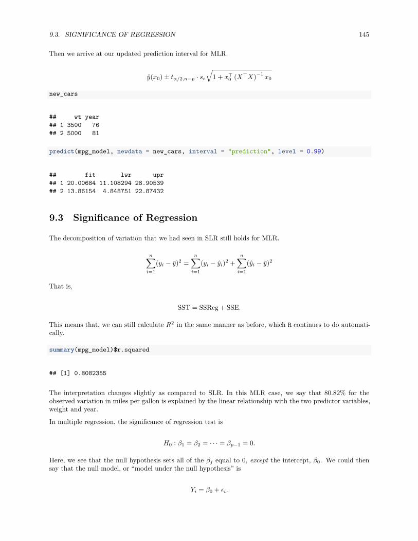
9.3. SIGNIFICANCE OF REGRESSION 145
Then we arrive at our updated prediction interval for MLR.
y(x0) ± tα/2,n−p · se
√1 + x⊤
0 (X⊤X)−1x0
new_cars
## wt year## 1 3500 76## 2 5000 81
predict(mpg_model, newdata = new_cars, interval = "prediction", level = 0.99)
## fit lwr upr## 1 20.00684 11.108294 28.90539## 2 13.86154 4.848751 22.87432
9.3 Significance of Regression
The decomposition of variation that we had seen in SLR still holds for MLR.
n∑i=1
(yi − y)2 =n∑
i=1(yi − yi)2 +
n∑i=1
(yi − y)2
That is,
SST = SSReg + SSE.
This means that, we can still calculate R2 in the same manner as before, which R continues to do automati-cally.
summary(mpg_model)$r.squared
## [1] 0.8082355
The interpretation changes slightly as compared to SLR. In this MLR case, we say that 80.82% for theobserved variation in miles per gallon is explained by the linear relationship with the two predictor variables,weight and year.
In multiple regression, the significance of regression test is
H0 : β1 = β2 = · · · = βp−1 = 0.
Here, we see that the null hypothesis sets all of the βj equal to 0, except the intercept, β0. We could thensay that the null model, or “model under the null hypothesis” is
Yi = β0 + ϵi.
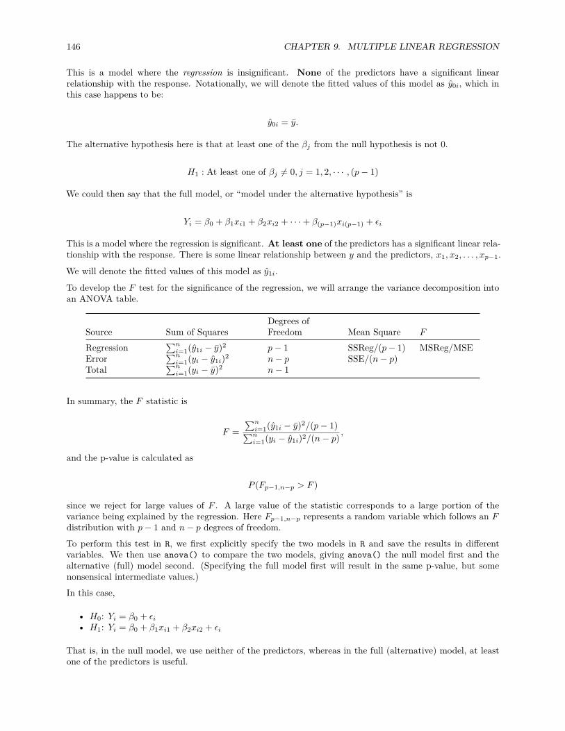
146 CHAPTER 9. MULTIPLE LINEAR REGRESSION
This is a model where the regression is insignificant. None of the predictors have a significant linearrelationship with the response. Notationally, we will denote the fitted values of this model as y0i, which inthis case happens to be:
y0i = y.
The alternative hypothesis here is that at least one of the βj from the null hypothesis is not 0.
H1 : At least one of βj = 0, j = 1, 2, · · · , (p − 1)
We could then say that the full model, or “model under the alternative hypothesis” is
Yi = β0 + β1xi1 + β2xi2 + · · · + β(p−1)xi(p−1) + ϵi
This is a model where the regression is significant. At least one of the predictors has a significant linear rela-tionship with the response. There is some linear relationship between y and the predictors, x1, x2, . . . , xp−1.
We will denote the fitted values of this model as y1i.
To develop the F test for the significance of the regression, we will arrange the variance decomposition intoan ANOVA table.
Source Sum of SquaresDegrees ofFreedom Mean Square F
Regression∑n
i=1(y1i − y)2 p − 1 SSReg/(p − 1) MSReg/MSEError
∑ni=1(yi − y1i)2 n − p SSE/(n − p)
Total∑n
i=1(yi − y)2 n − 1
In summary, the F statistic is
F =∑n
i=1(y1i − y)2/(p − 1)∑ni=1(yi − y1i)2/(n − p)
,
and the p-value is calculated as
P (Fp−1,n−p > F )
since we reject for large values of F . A large value of the statistic corresponds to a large portion of thevariance being explained by the regression. Here Fp−1,n−p represents a random variable which follows an Fdistribution with p − 1 and n − p degrees of freedom.To perform this test in R, we first explicitly specify the two models in R and save the results in differentvariables. We then use anova() to compare the two models, giving anova() the null model first and thealternative (full) model second. (Specifying the full model first will result in the same p-value, but somenonsensical intermediate values.)In this case,
• H0: Yi = β0 + ϵi
• H1: Yi = β0 + β1xi1 + β2xi2 + ϵi
That is, in the null model, we use neither of the predictors, whereas in the full (alternative) model, at leastone of the predictors is useful.
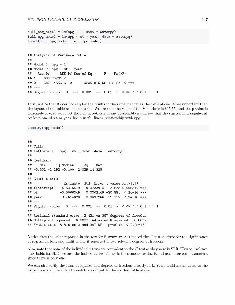
9.3. SIGNIFICANCE OF REGRESSION 147
null_mpg_model = lm(mpg ~ 1, data = autompg)full_mpg_model = lm(mpg ~ wt + year, data = autompg)anova(null_mpg_model, full_mpg_model)
## Analysis of Variance Table#### Model 1: mpg ~ 1## Model 2: mpg ~ wt + year## Res.Df RSS Df Sum of Sq F Pr(>F)## 1 389 23761.7## 2 387 4556.6 2 19205 815.55 < 2.2e-16 ***## ---## Signif. codes: 0 '***' 0.001 '**' 0.01 '*' 0.05 '.' 0.1 ' ' 1
First, notice that R does not display the results in the same manner as the table above. More important thanthe layout of the table are its contents. We see that the value of the F statistic is 815.55, and the p-value isextremely low, so we reject the null hypothesis at any reasonable α and say that the regression is significant.At least one of wt or year has a useful linear relationship with mpg.
summary(mpg_model)
#### Call:## lm(formula = mpg ~ wt + year, data = autompg)#### Residuals:## Min 1Q Median 3Q Max## -8.852 -2.292 -0.100 2.039 14.325#### Coefficients:## Estimate Std. Error t value Pr(>|t|)## (Intercept) -14.6376419 4.0233914 -3.638 0.000312 ***## wt -0.0066349 0.0002149 -30.881 < 2e-16 ***## year 0.7614020 0.0497266 15.312 < 2e-16 ***## ---## Signif. codes: 0 '***' 0.001 '**' 0.01 '*' 0.05 '.' 0.1 ' ' 1#### Residual standard error: 3.431 on 387 degrees of freedom## Multiple R-squared: 0.8082, Adjusted R-squared: 0.8072## F-statistic: 815.6 on 2 and 387 DF, p-value: < 2.2e-16
Notice that the value reported in the row for F-statistic is indeed the F test statistic for the significanceof regression test, and additionally it reports the two relevant degrees of freedom.
Also, note that none of the individual t-tests are equivalent to the F -test as they were in SLR. This equivalenceonly holds for SLR because the individual test for β1 is the same as testing for all non-intercept parameters,since there is only one.
We can also verify the sums of squares and degrees of freedom directly in R. You should match these to thetable from R and use this to match R’s output to the written table above.

148 CHAPTER 9. MULTIPLE LINEAR REGRESSION
# SSRegsum((fitted(full_mpg_model) - fitted(null_mpg_model)) ^ 2)
## [1] 19205.03
# SSEsum(resid(full_mpg_model) ^ 2)
## [1] 4556.646
# SSTsum(resid(null_mpg_model) ^ 2)
## [1] 23761.67
# Degrees of Freedom: Regressionlength(coef(full_mpg_model)) - length(coef(null_mpg_model))
## [1] 2
# Degrees of Freedom: Errorlength(resid(full_mpg_model)) - length(coef(full_mpg_model))
## [1] 387
# Degrees of Freedom: Totallength(resid(null_mpg_model)) - length(coef(null_mpg_model))
## [1] 389
9.4 Nested Models
The significance of regression test is actually a special case of testing what we will call nested models.More generally we can compare two models, where one model is “nested” inside the other, meaning onemodel contains a subset of the predictors from only the larger model.
Consider the following full model,
Yi = β0 + β1xi1 + β2xi2 + · · · + β(p−1)xi(p−1) + ϵi
This model has p − 1 predictors, for a total of p β-parameters. We will denote the fitted values of this modelas y1i.
Let the null model be
Yi = β0 + β1xi1 + β2xi2 + · · · + β(q−1)xi(q−1) + ϵi
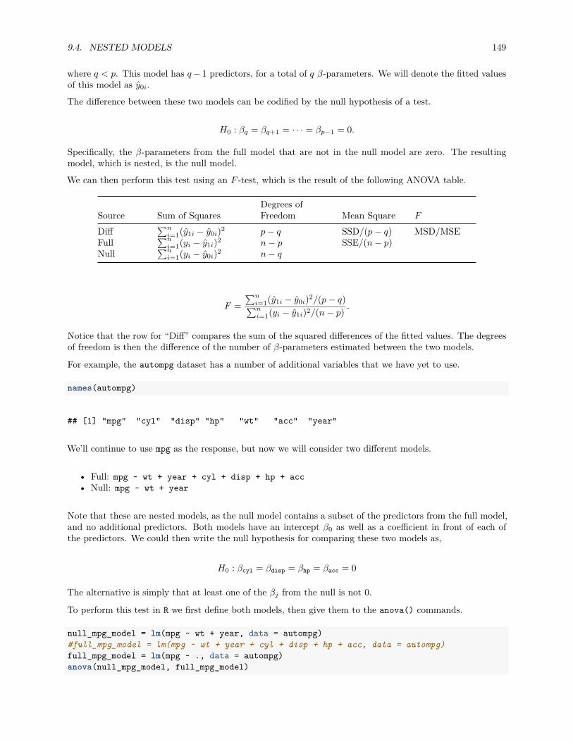
9.4. NESTED MODELS 149
where q < p. This model has q − 1 predictors, for a total of q β-parameters. We will denote the fitted valuesof this model as y0i.
The difference between these two models can be codified by the null hypothesis of a test.
H0 : βq = βq+1 = · · · = βp−1 = 0.
Specifically, the β-parameters from the full model that are not in the null model are zero. The resultingmodel, which is nested, is the null model.
We can then perform this test using an F -test, which is the result of the following ANOVA table.
Source Sum of SquaresDegrees ofFreedom Mean Square F
Diff∑n
i=1(y1i − y0i)2 p − q SSD/(p − q) MSD/MSEFull
∑ni=1(yi − y1i)2 n − p SSE/(n − p)
Null∑n
i=1(yi − y0i)2 n − q
F =∑n
i=1(y1i − y0i)2/(p − q)∑ni=1(yi − y1i)2/(n − p)
.
Notice that the row for “Diff” compares the sum of the squared differences of the fitted values. The degreesof freedom is then the difference of the number of β-parameters estimated between the two models.
For example, the autompg dataset has a number of additional variables that we have yet to use.
names(autompg)
## [1] "mpg" "cyl" "disp" "hp" "wt" "acc" "year"
We’ll continue to use mpg as the response, but now we will consider two different models.
• Full: mpg ~ wt + year + cyl + disp + hp + acc• Null: mpg ~ wt + year
Note that these are nested models, as the null model contains a subset of the predictors from the full model,and no additional predictors. Both models have an intercept β0 as well as a coefficient in front of each ofthe predictors. We could then write the null hypothesis for comparing these two models as,
H0 : βcyl = βdisp = βhp = βacc = 0
The alternative is simply that at least one of the βj from the null is not 0.
To perform this test in R we first define both models, then give them to the anova() commands.
null_mpg_model = lm(mpg ~ wt + year, data = autompg)#full_mpg_model = lm(mpg ~ wt + year + cyl + disp + hp + acc, data = autompg)full_mpg_model = lm(mpg ~ ., data = autompg)anova(null_mpg_model, full_mpg_model)

150 CHAPTER 9. MULTIPLE LINEAR REGRESSION
## Analysis of Variance Table#### Model 1: mpg ~ wt + year## Model 2: mpg ~ cyl + disp + hp + wt + acc + year## Res.Df RSS Df Sum of Sq F Pr(>F)## 1 387 4556.6## 2 383 4530.5 4 26.18 0.5533 0.6967
Here we have used the formula mpg ~ . to define to full model. This is the same as the commented outline. Specifically, this a common shortcut in R which reads, “model mpg as the response with each of theremaining variables in the data frame as predictors.”
Here we see that the value of the F statistic is 0.553, and the p-value is very large, so we fail to reject thenull hypothesis at any reasonable α and say that none of cyl, disp, hp, and acc are significant with wt andyear already in the model.
Again, we verify the sums of squares and degrees of freedom directly in R. You should match these to thetable from R, and use this to match R’s output to the written table above.
# SSDiffsum((fitted(full_mpg_model) - fitted(null_mpg_model)) ^ 2)
## [1] 26.17981
# SSE (For Full)sum(resid(full_mpg_model) ^ 2)
## [1] 4530.466
# SST (For Null)sum(resid(null_mpg_model) ^ 2)
## [1] 4556.646
# Degrees of Freedom: Difflength(coef(full_mpg_model)) - length(coef(null_mpg_model))
## [1] 4
# Degrees of Freedom: Fulllength(resid(full_mpg_model)) - length(coef(full_mpg_model))
## [1] 383
# Degrees of Freedom: Nulllength(resid(null_mpg_model)) - length(coef(null_mpg_model))
## [1] 387

9.5. SIMULATION 151
9.5 Simulation
Since we ignored the derivation of certain results, we will again use simulation to convince ourselves of someof the above results. In particular, we will simulate samples of size n = 100 from the model
Yi = 5 + −2xi1 + 6xi2 + ϵi, i = 1, 2, . . . , n
where ϵi ∼ N(0, σ2 = 16). Here we have two predictors, so p = 3.
set.seed(1337)n = 100 # sample sizep = 3
beta_0 = 5beta_1 = -2beta_2 = 6sigma = 4
As is the norm with regression, the x values are considered fixed and known quantities, so we will simulatethose first, and they remain the same for the rest of the simulation study. Also note we create an x0 whichis all 1, which we need to create our X matrix. If you look at the matrix formulation of regression, this unitvector of all 1s is a “predictor” that puts the intercept into the model. We also calculate the C matrix forlater use.
x0 = rep(1, n)x1 = sample(seq(1, 10, length = n))x2 = sample(seq(1, 10, length = n))X = cbind(x0, x1, x2)C = solve(t(X) %*% X)
We then simulate the response according the model above. Lastly, we place the two predictors and responseinto a data frame. Note that we do not place x0 in the data frame. This is a result of R adding an interceptby default.
eps = rnorm(n, mean = 0, sd = sigma)y = beta_0 + beta_1 * x1 + beta_2 * x2 + epssim_data = data.frame(x1, x2, y)
Plotting this data and fitting the regression produces the following plot.
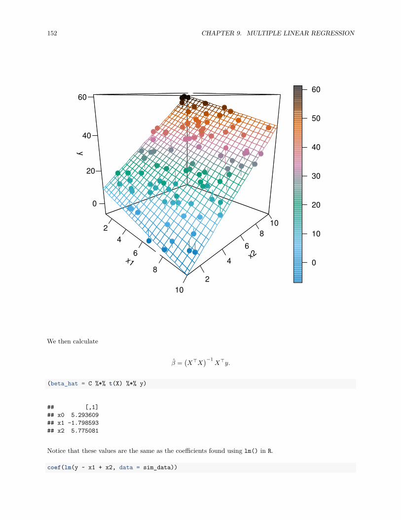
152 CHAPTER 9. MULTIPLE LINEAR REGRESSION
x1
24
6
8
10
x2
2
4
6
810
y
0
20
40
60
0
10
20
30
40
50
60
We then calculate
β =(X⊤X
)−1X⊤y.
(beta_hat = C %*% t(X) %*% y)
## [,1]## x0 5.293609## x1 -1.798593## x2 5.775081
Notice that these values are the same as the coefficients found using lm() in R.
coef(lm(y ~ x1 + x2, data = sim_data))
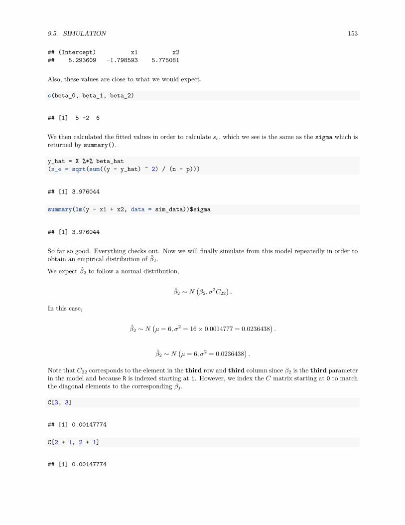
9.5. SIMULATION 153
## (Intercept) x1 x2## 5.293609 -1.798593 5.775081
Also, these values are close to what we would expect.
c(beta_0, beta_1, beta_2)
## [1] 5 -2 6
We then calculated the fitted values in order to calculate se, which we see is the same as the sigma which isreturned by summary().
y_hat = X %*% beta_hat(s_e = sqrt(sum((y - y_hat) ^ 2) / (n - p)))
## [1] 3.976044
summary(lm(y ~ x1 + x2, data = sim_data))$sigma
## [1] 3.976044
So far so good. Everything checks out. Now we will finally simulate from this model repeatedly in order toobtain an empirical distribution of β2.
We expect β2 to follow a normal distribution,
β2 ∼ N(β2, σ2C22
).
In this case,
β2 ∼ N(µ = 6, σ2 = 16 × 0.0014777 = 0.0236438
).
β2 ∼ N(µ = 6, σ2 = 0.0236438
).
Note that C22 corresponds to the element in the third row and third column since β2 is the third parameterin the model and because R is indexed starting at 1. However, we index the C matrix starting at 0 to matchthe diagonal elements to the corresponding βj .
C[3, 3]
## [1] 0.00147774
C[2 + 1, 2 + 1]
## [1] 0.00147774

154 CHAPTER 9. MULTIPLE LINEAR REGRESSION
sigma ^ 2 * C[2 + 1, 2 + 1]
## [1] 0.02364383
We now perform the simulation a large number of times. Each time, we update the y variable in the dataframe, leaving the x variables the same. We then fit a model, and store β2.
num_sims = 10000beta_hat_2 = rep(0, num_sims)for(i in 1:num_sims) {eps = rnorm(n, mean = 0 , sd = sigma)sim_data$y = beta_0 * x0 + beta_1 * x1 + beta_2 * x2 + epsfit = lm(y ~ x1 + x2, data = sim_data)beta_hat_2[i] = coef(fit)[3]
}
We then see that the mean of the simulated values is close to the true value of β2.
mean(beta_hat_2)
## [1] 5.99871
beta_2
## [1] 6
We also see that the variance of the simulated values is close to the true variance of β2.
Var[β2] = σ2 · C22 = 16 × 0.0014777 = 0.0236438
var(beta_hat_2)
## [1] 0.02360853
sigma ^ 2 * C[2 + 1, 2 + 1]
## [1] 0.02364383
The standard deviations found from the simulated data and the parent population are also very close.
sd(beta_hat_2)
## [1] 0.1536507
sqrt(sigma ^ 2 * C[2 + 1, 2 + 1])
## [1] 0.1537655
Lastly, we plot a histogram of the simulated values, and overlay the true distribution.
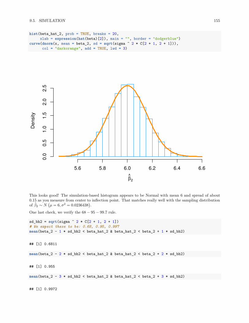
9.5. SIMULATION 155
hist(beta_hat_2, prob = TRUE, breaks = 20,xlab = expression(hat(beta)[2]), main = "", border = "dodgerblue")
curve(dnorm(x, mean = beta_2, sd = sqrt(sigma ^ 2 * C[2 + 1, 2 + 1])),col = "darkorange", add = TRUE, lwd = 3)
β2
Den
sity
5.6 5.8 6.0 6.2 6.4 6.6
0.0
0.5
1.0
1.5
2.0
2.5
This looks good! The simulation-based histogram appears to be Normal with mean 6 and spread of about0.15 as you measure from center to inflection point. That matches really well with the sampling distributionof β2 ∼ N
(µ = 6, σ2 = 0.0236438
).
One last check, we verify the 68 − 95 − 99.7 rule.
sd_bh2 = sqrt(sigma ^ 2 * C[2 + 1, 2 + 1])# We expect these to be: 0.68, 0.95, 0.997mean(beta_2 - 1 * sd_bh2 < beta_hat_2 & beta_hat_2 < beta_2 + 1 * sd_bh2)
## [1] 0.6811
mean(beta_2 - 2 * sd_bh2 < beta_hat_2 & beta_hat_2 < beta_2 + 2 * sd_bh2)
## [1] 0.955
mean(beta_2 - 3 * sd_bh2 < beta_hat_2 & beta_hat_2 < beta_2 + 3 * sd_bh2)
## [1] 0.9972

156 CHAPTER 9. MULTIPLE LINEAR REGRESSION
Chapter 10
Model Building
“Statisticians, like artists, have the bad habit of falling in love with their models.”— George Box
Let’s take a step back and consider the process of finding a model for data at a higher level. We areattempting to find a model for a response variable y based on a number of predictors x1, x2, x3, . . . , xp−1.Essentially, we are trying to discover the functional relationship between y and the predictors. In the previouschapter we were fitting models for a car’s fuel efficiency (mpg) as a function of its attributes (wt, year, cyl,disp, hp, acc). We also consider y to be a function of some noise. Rarely if ever do we expect there to bean exact functional relationship between the predictors and the response.
y = f(x1, x2, x3, . . . , xp−1) + ϵ
We can think of this as
response = signal + noise.
We could consider all sorts of complicated functions for f . You will likely encounter several ways of doingthis in future machine learning courses. So far in this course we have focused on (multiple) linear regression.That is
y = f(x1, x2, x3, . . . , xp−1) + ϵ
= β0 + β1x1 + β2x2 + · · · + βp−1xp−1 + ϵ
In the big picture of possible models that we could fit to this data, this is a rather restrictive model. Whatdo we mean by a restrictive model?
10.1 Family, Form, and Fit
When modeling data, there are a number of choices that need to be made.
• What family of models will be considered?• What form of the model will be used?• How will the model be fit?
Let’s work backwards and discuss each of these.
157

158 CHAPTER 10. MODEL BUILDING
10.1.1 Fit
Consider one of the simplest models we could fit to data, simple linear regression.
y = f(x1, x2, x3, . . . , xp−1) + ϵ = β0 + β1x1 + ϵ
So here, despite having multiple predictors, we chose to use only one. How is this model fit? We will almostexclusively use the method of least squares, but recall, we had seen alternative methods of fitting this model.
argminβ0,β1
max |yi − (β0 + β1xi)|
argminβ0,β1
n∑i=1
|yi − (β0 + β1xi)|
argminβ0,β1
n∑i=1
(yi − (β0 + β1xi))2
Any of these methods (we will always use the last, least squares) will obtain estimates of the unknownparameters β0 and β1. Since those are the only unknowns of the specified model, we have then fit the model.The fitted model is then
y = f(x1, x2, x3, . . . , xp−1) = β0 + β1x1
Note that, now we have dropped the term for the noise. We don’t make any effort to model the noise, onlythe signal.
10.1.2 Form
What are the different forms a model could take? Currently, for the linear models we have considered, theonly method for altering the form of the model is to control the predictors used. For example, one form ofthe multiple linear regression model is simple linear regression.
y = f(x1, x2, x3, . . . , xp−1) + ϵ = β0 + β1x1 + ϵ
We could also consider a SLR model with a different predictor, thus altering the form of the model.
y = f(x1, x2, x3, . . . , xp−1) + ϵ = β0 + β2x2 + ϵ
Often, we’ll use multiple predictors in our model. Very often, we will at least try a model with all possiblepredictors.
y = f(x1, x2, x3, . . . , xp−1) + ϵ
= β0 + β1x1 + β2x2 + · · · + βp−1xp−1 + ϵ
We could also use some, but not all of the predictors.
y = f(x1, x2, x3, . . . , xp−1) + ϵ
= β0 + β1x1 + β3x3 + β5x5 + ϵ
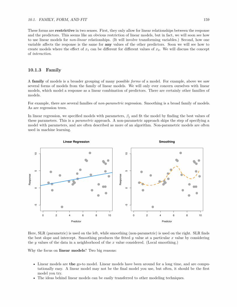
10.1. FAMILY, FORM, AND FIT 159
These forms are restrictive in two senses. First, they only allow for linear relationships between the responseand the predictors. This seems like an obvious restriction of linear models, but in fact, we will soon see howto use linear models for non-linear relationships. (It will involve transforming variables.) Second, how onevariable affects the response is the same for any values of the other predictors. Soon we will see how tocreate models where the effect of x1 can be different for different values of x2. We will discuss the conceptof interaction.
10.1.3 Family
A family of models is a broader grouping of many possible forms of a model. For example, above we sawseveral forms of models from the family of linear models. We will only ever concern ourselves with linearmodels, which model a response as a linear combination of predictors. There are certainly other families ofmodels.
For example, there are several families of non-parametric regression. Smoothing is a broad family of models.As are regression trees.
In linear regression, we specified models with parameters, βj and fit the model by finding the best values ofthese parameters. This is a parametric approach. A non-parametric approach skips the step of specifying amodel with parameters, and are often described as more of an algorithm. Non-parametric models are oftenused in machine learning.
0 2 4 6 8 10
-50
510
Linear Regression
Predictor
Res
pons
e
0 2 4 6 8 10
-50
510
Smoothing
Predictor
Res
pons
e
Here, SLR (parametric) is used on the left, while smoothing (non-parametric) is used on the right. SLR findsthe best slope and intercept. Smoothing produces the fitted y value at a particular x value by consideringthe y values of the data in a neighborhood of the x value considered. (Local smoothing.)
Why the focus on linear models? Two big reasons:
• Linear models are the go-to model. Linear models have been around for a long time, and are compu-tationally easy. A linear model may not be the final model you use, but often, it should be the firstmodel you try.
• The ideas behind linear models can be easily transferred to other modeling techniques.
160 CHAPTER 10. MODEL BUILDING
10.1.4 Assumed Model, Fitted Model
When searching for a model, we often need to make assumptions. These assumptions are codified in thefamily and form of the model. For example
y = β0 + β1x1 + β3x3 + β5x5 + ϵ
assumes that y is a linear combination of x1, x3, and x5 as well as some noise. This assumes that the effectof x1 on y is β1, which is the same for all values of x3 and x5. That is, we are using the family of linearmodels with a particular form.
Suppose we then fit this model to some data and obtain the fitted model. For example, in R we would use
fit = lm(y ~ x1 + x3 + x5, data = some_data)
This is R’s way of saying the family is linear and specifying the form from above. An additive model withthe specified predictors as well as an intercept. We then obtain
y = 1.5 + 0.9x1 + 1.1x3 + 2.3x5.
This is our best guess for the function f in
y = f(x1, x2, x3, . . . , xp−1) + ϵ
for the assumed family and form. Fitting a model only gives us the best fit for the family and form thatwe specify. So the natural question is; how to we choose the correct family and form? We’ll focus on formsince we are focusing on the family of linear models.
10.2 Explanation versus Prediction
What is the purpose of fitting a model to data? Usually it is to accomplish one of two goals. We can usea model to explain the relationship between the response and the predictors. Models can also be used topredict the response based on the predictors. Often, a good model will do both, but we’ll discuss both goalsseparately since the process of finding models for explaining and predicting have some differences.
For our purposes, since we are only considering linear models, searching for a good model is essentiallysearching for a good form of a model.
10.2.1 Explanation
If the goal of a model is to explain the relationship between the response and the predictors, we are lookingfor a model that is small and interpretable, but still fits the data well. When discussing linear models,the size of a model is essentially the number of β parameters used.
Suppose we would like to find a model that explains fuel efficiency (mpg) based on a car’s attributes (wt,year, cyl, disp, hp, acc). Perhaps we are a car manufacturer trying to engineer a fuel efficient vehicle. Ifthis is the case, we are interested in both which predictor variables are useful for explaining the car’s fuelefficiency, as well as how those variables effect fuel efficiency. By understanding this relationship, we can usethis knowledge to our advantage when designing a car.
To explain a relationship, we are interested in keeping models as small as possible, since smaller models areeasy to interpret. The fewer predictors the less considerations we need to make in our design process.

10.2. EXPLANATION VERSUS PREDICTION 161
Note that linear models of any size are rather interpretable to begin with. Later in your data analysis careers,you will see more complicated models that may fit data better, but are much harder, if not impossible tointerpret. These models aren’t nearly as useful for explaining a relationship. This is another reason to alwaysattempt a linear model. If it fits as well as more complicated methods, it will be the easiest to understand.
To find small and interpretable models, we will eventually use selection procedures, which search among manypossible forms of a model. For now we will do this in a more ad-hoc manner using inference techniques wehave already encountered. To use inference as we have seen it, we need an additional assumption in additionto the family and form of the model.
y = β0 + β1x1 + β3x3 + β5x5 + ϵ
Our additional assumption is about the error term.
ϵ ∼ N(0, σ2)
This assumption, that the errors are normally distributed with some common variance is the key to all ofthe inference we have done so far. We will discuss this is great detail later.
So with our inference tools (ANOVA and t-test) we have two potential strategies. Start with a very smallmodel (no predictors) and attempt to add predictors. Or, start with a big model (all predictors) and attemptto remove predictors.
10.2.1.1 Correlation and Causation
A word of caution when using a model to explain a relationship. There are two terms often used to describea relationship between two variables: causation and correlation. Correlation is often also referred to asassociation.
Just because two variables are correlated does not necessarily mean that one causes the other. For example,consider modeling mpg as only a function of hp.
plot(mpg ~ hp, data = autompg, col = "dodgerblue", pch = 20, cex = 1.5)
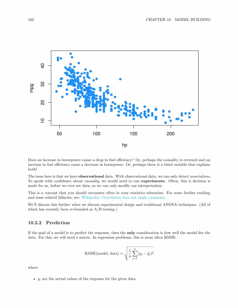
162 CHAPTER 10. MODEL BUILDING
50 100 150 200
1020
3040
hp
mpg
Does an increase in horsepower cause a drop in fuel efficiency? Or, perhaps the causality is reversed and anincrease in fuel efficiency cause a decrease in horsepower. Or, perhaps there is a third variable that explainsboth!
The issue here is that we have observational data. With observational data, we can only detect associations.To speak with confidence about causality, we would need to run experiments. Often, this is decision ismade for us, before we ever see data, so we can only modify our interpretation.
This is a concept that you should encounter often in your statistics education. For some further reading,and some related fallacies, see: Wikipedia: Correlation does not imply causation.
We’ll discuss this further when we discuss experimental design and traditional ANOVA techniques. (All ofwhich has recently been re-branded as A/B testing.)
10.2.2 Prediction
If the goal of a model is to predict the response, then the only consideration is how well the model fits thedata. For this, we will need a metric. In regression problems, this is most often RMSE.
RMSE(model, data) =
√√√√ 1n
n∑i=1
(yi − yi)2
where
• yi are the actual values of the response for the given data

10.2. EXPLANATION VERSUS PREDICTION 163
• yi are the predicted values using the fitted model and the predictors from the data
Correlation and causation are not an issue here. If a predictor is correlated with the response, it is usefulfor prediction. For example, in elementary school aged children their shoe size certainly doesn’t cause themto read at a higher level, however we could very easily use shoe size to make a prediction about a child’sreading ability. The larger their shoe size, the better they read. There’s a lurking variable here though, theirage! (Don’t send your kids to school with size 14 shoes, it won’t make them read better!)
Also, since we are not performing inference, the extra assumption about the errors is not needed. The onlything we care about is how close the fitted model is to the data. Least squares is least squares. For aspecified model, it will find the values of the parameters which will minimize the squared error loss. Yourresults might be largely uninterpretable and useless for inference, but for prediction none of that matters.
Suppose instead of the manufacturer who would like to build a car, we are a consumer who wishes to purchasea new car. However this particular car is so new, it has not been rigorously tested, so we are unsure of whatfuel efficiency to expect. (And, as skeptics, we don’t trust what the manufacturer is telling us.) In this case,we would like to use the model to help predict the fuel efficiency of this car based on its attributes, whichare the predictors of the model. The smaller the errors the model makes, the more confident we are in itsprediction.
10.2.2.1 Test-Train Split
The trouble with using RMSE to identify how well a model fits data, is that RMSE is always (equal or)lower for a larger model. This would suggest that we should always use the largest model possible whenlooking for a model that predicts well. The problem with this is the potential to overfit to the data. So, wewant a model that fits well, but does not overfit. To understand overfitting, we need to think about applyinga model to seen and unseen data.
Suppose we fit a model using all data available and we evaluate RMSE on this fitted model and all of theseen data. We will call this data the training data, and this RMSE the train RMSE.
Now, suppose we magically encounter some additional additional data. To truly asses how well the modelpredicts, we should evaluate how well our models predicts the response of this data. We will call this datathe test data and this RMSE the test RMSE.
• Train RMSE: model fit on seen data, evaluated on seen data• Test RMSE: model fit on seen data, evaluated on unseen data
Below, we simulate some data and fit two models. We will call the solid blue line the “simple” model. Thedashed orange line will be called the “complex” model, which was fit with methods we do not yet know.
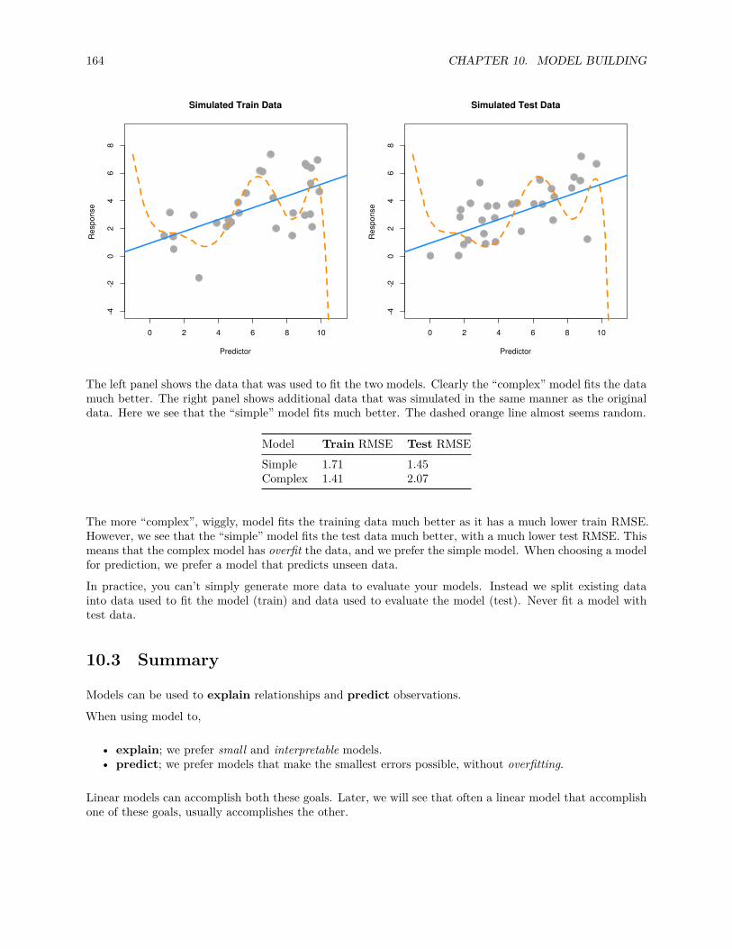
164 CHAPTER 10. MODEL BUILDING
0 2 4 6 8 10
-4-2
02
46
8Simulated Train Data
Predictor
Res
pons
e
0 2 4 6 8 10
-4-2
02
46
8
Simulated Test Data
Predictor
Res
pons
e
The left panel shows the data that was used to fit the two models. Clearly the “complex” model fits the datamuch better. The right panel shows additional data that was simulated in the same manner as the originaldata. Here we see that the “simple” model fits much better. The dashed orange line almost seems random.
Model Train RMSE Test RMSESimple 1.71 1.45Complex 1.41 2.07
The more “complex”, wiggly, model fits the training data much better as it has a much lower train RMSE.However, we see that the “simple” model fits the test data much better, with a much lower test RMSE. Thismeans that the complex model has overfit the data, and we prefer the simple model. When choosing a modelfor prediction, we prefer a model that predicts unseen data.
In practice, you can’t simply generate more data to evaluate your models. Instead we split existing datainto data used to fit the model (train) and data used to evaluate the model (test). Never fit a model withtest data.
10.3 Summary
Models can be used to explain relationships and predict observations.
When using model to,
• explain; we prefer small and interpretable models.• predict; we prefer models that make the smallest errors possible, without overfitting.
Linear models can accomplish both these goals. Later, we will see that often a linear model that accomplishone of these goals, usually accomplishes the other.

Chapter 11
Categorical Predictors andInteractions
“The greatest value of a picture is when it forces us to notice what we never expected to see.”— John Tukey
After reading this chapter you will be able to:
• Include and interpret categorical variables in a linear regression model by way of dummy variables.• Understand the implications of using a model with a categorical variable in two ways: levels serving
as unique predictors versus levels serving as a comparison to a baseline.• Construct and interpret linear regression models with interaction terms.• Identify categorical variables in a data set and convert them into factor variables, if necessary, using
R.
So far in each of our analyses, we have only used numeric variables as predictors. We have also only usedadditive models, meaning the effect any predictor had on the response was not dependent on the otherpredictors. In this chapter, we will remove both of these restrictions. We will fit models with categoricalpredictors, and use models that allow predictors to interact. The mathematics of multiple regression willremain largely unchanging, however, we will pay close attention to interpretation, as well as some differencein R usage.
11.1 Dummy Variables
For this chapter, we will briefly use the built in dataset mtcars before returning to our autompg dataset thatwe created in the last chapter. The mtcars dataset is somewhat smaller, so we’ll quickly take a look at theentire dataset.
mtcars
## mpg cyl disp hp drat wt qsec vs am gear carb## Mazda RX4 21.0 6 160.0 110 3.90 2.620 16.46 0 1 4 4## Mazda RX4 Wag 21.0 6 160.0 110 3.90 2.875 17.02 0 1 4 4## Datsun 710 22.8 4 108.0 93 3.85 2.320 18.61 1 1 4 1## Hornet 4 Drive 21.4 6 258.0 110 3.08 3.215 19.44 1 0 3 1
165

166 CHAPTER 11. CATEGORICAL PREDICTORS AND INTERACTIONS
## Hornet Sportabout 18.7 8 360.0 175 3.15 3.440 17.02 0 0 3 2## Valiant 18.1 6 225.0 105 2.76 3.460 20.22 1 0 3 1## Duster 360 14.3 8 360.0 245 3.21 3.570 15.84 0 0 3 4## Merc 240D 24.4 4 146.7 62 3.69 3.190 20.00 1 0 4 2## Merc 230 22.8 4 140.8 95 3.92 3.150 22.90 1 0 4 2## Merc 280 19.2 6 167.6 123 3.92 3.440 18.30 1 0 4 4## Merc 280C 17.8 6 167.6 123 3.92 3.440 18.90 1 0 4 4## Merc 450SE 16.4 8 275.8 180 3.07 4.070 17.40 0 0 3 3## Merc 450SL 17.3 8 275.8 180 3.07 3.730 17.60 0 0 3 3## Merc 450SLC 15.2 8 275.8 180 3.07 3.780 18.00 0 0 3 3## Cadillac Fleetwood 10.4 8 472.0 205 2.93 5.250 17.98 0 0 3 4## Lincoln Continental 10.4 8 460.0 215 3.00 5.424 17.82 0 0 3 4## Chrysler Imperial 14.7 8 440.0 230 3.23 5.345 17.42 0 0 3 4## Fiat 128 32.4 4 78.7 66 4.08 2.200 19.47 1 1 4 1## Honda Civic 30.4 4 75.7 52 4.93 1.615 18.52 1 1 4 2## Toyota Corolla 33.9 4 71.1 65 4.22 1.835 19.90 1 1 4 1## Toyota Corona 21.5 4 120.1 97 3.70 2.465 20.01 1 0 3 1## Dodge Challenger 15.5 8 318.0 150 2.76 3.520 16.87 0 0 3 2## AMC Javelin 15.2 8 304.0 150 3.15 3.435 17.30 0 0 3 2## Camaro Z28 13.3 8 350.0 245 3.73 3.840 15.41 0 0 3 4## Pontiac Firebird 19.2 8 400.0 175 3.08 3.845 17.05 0 0 3 2## Fiat X1-9 27.3 4 79.0 66 4.08 1.935 18.90 1 1 4 1## Porsche 914-2 26.0 4 120.3 91 4.43 2.140 16.70 0 1 5 2## Lotus Europa 30.4 4 95.1 113 3.77 1.513 16.90 1 1 5 2## Ford Pantera L 15.8 8 351.0 264 4.22 3.170 14.50 0 1 5 4## Ferrari Dino 19.7 6 145.0 175 3.62 2.770 15.50 0 1 5 6## Maserati Bora 15.0 8 301.0 335 3.54 3.570 14.60 0 1 5 8## Volvo 142E 21.4 4 121.0 109 4.11 2.780 18.60 1 1 4 2
We will be interested in three of the variables: mpg, hp, and am.
• mpg: fuel efficiency, in miles per gallon.• hp: horsepower, in foot-pounds per second.• am: transmission. Automatic or manual.
As we often do, we will start by plotting the data. We are interested in mpg as the response variable, and hpas a predictor.
plot(mpg ~ hp, data = mtcars, cex = 2)
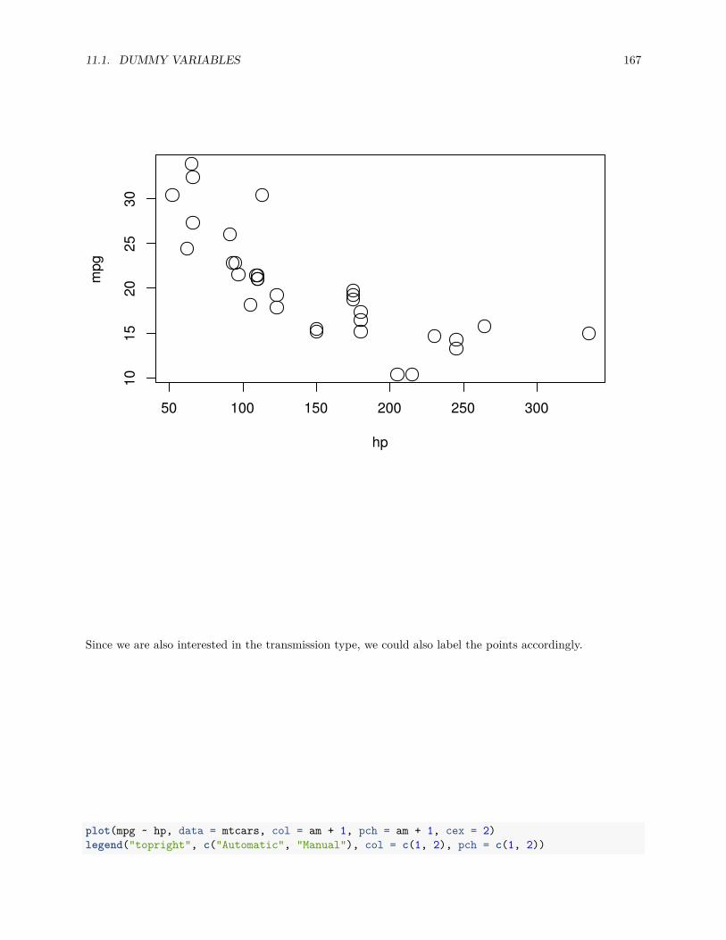
11.1. DUMMY VARIABLES 167
50 100 150 200 250 300
1015
2025
30
hp
mpg
Since we are also interested in the transmission type, we could also label the points accordingly.
plot(mpg ~ hp, data = mtcars, col = am + 1, pch = am + 1, cex = 2)legend("topright", c("Automatic", "Manual"), col = c(1, 2), pch = c(1, 2))
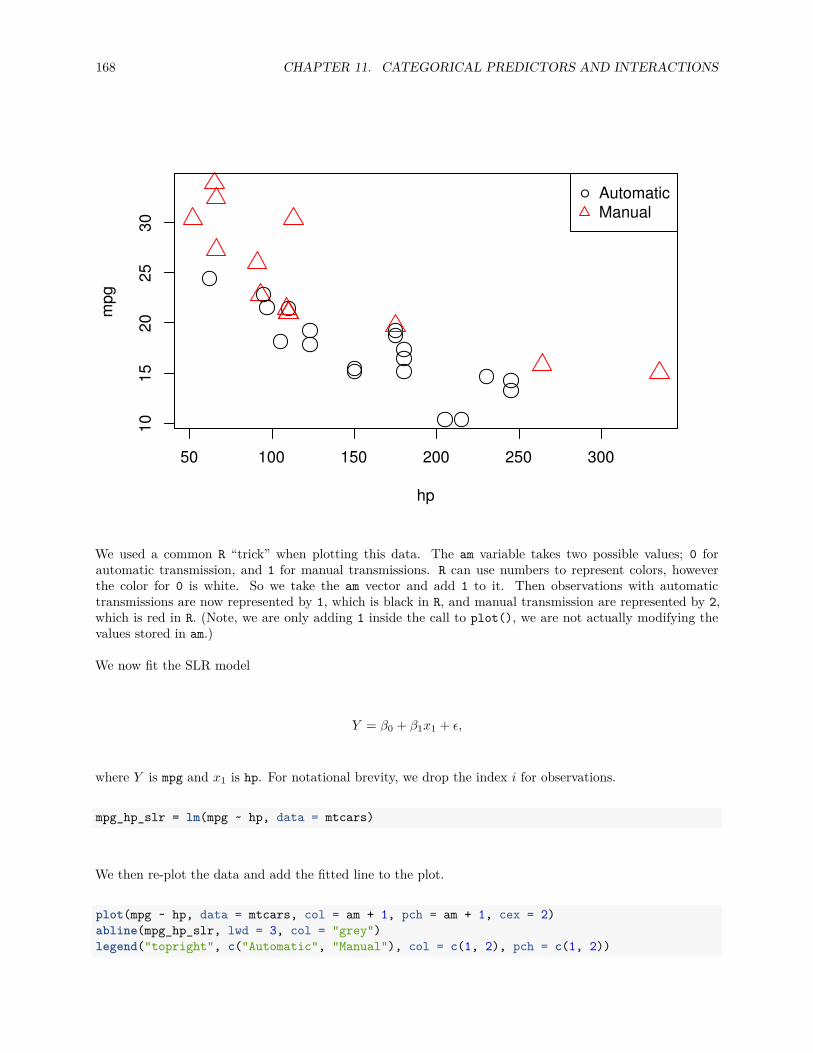
168 CHAPTER 11. CATEGORICAL PREDICTORS AND INTERACTIONS
50 100 150 200 250 300
1015
2025
30
hp
mpg
AutomaticManual
We used a common R “trick” when plotting this data. The am variable takes two possible values; 0 forautomatic transmission, and 1 for manual transmissions. R can use numbers to represent colors, howeverthe color for 0 is white. So we take the am vector and add 1 to it. Then observations with automatictransmissions are now represented by 1, which is black in R, and manual transmission are represented by 2,which is red in R. (Note, we are only adding 1 inside the call to plot(), we are not actually modifying thevalues stored in am.)
We now fit the SLR model
Y = β0 + β1x1 + ϵ,
where Y is mpg and x1 is hp. For notational brevity, we drop the index i for observations.
mpg_hp_slr = lm(mpg ~ hp, data = mtcars)
We then re-plot the data and add the fitted line to the plot.
plot(mpg ~ hp, data = mtcars, col = am + 1, pch = am + 1, cex = 2)abline(mpg_hp_slr, lwd = 3, col = "grey")legend("topright", c("Automatic", "Manual"), col = c(1, 2), pch = c(1, 2))
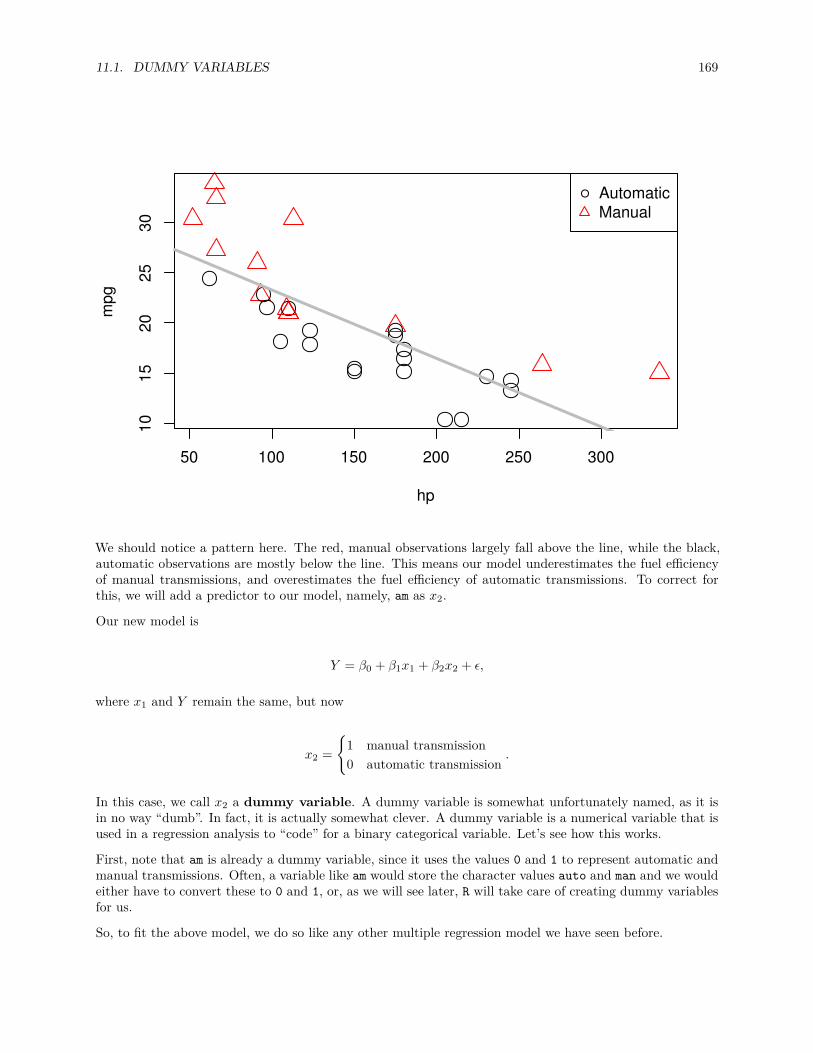
11.1. DUMMY VARIABLES 169
50 100 150 200 250 300
1015
2025
30
hp
mpg
AutomaticManual
We should notice a pattern here. The red, manual observations largely fall above the line, while the black,automatic observations are mostly below the line. This means our model underestimates the fuel efficiencyof manual transmissions, and overestimates the fuel efficiency of automatic transmissions. To correct forthis, we will add a predictor to our model, namely, am as x2.
Our new model is
Y = β0 + β1x1 + β2x2 + ϵ,
where x1 and Y remain the same, but now
x2 =
{1 manual transmission0 automatic transmission
.
In this case, we call x2 a dummy variable. A dummy variable is somewhat unfortunately named, as it isin no way “dumb”. In fact, it is actually somewhat clever. A dummy variable is a numerical variable that isused in a regression analysis to “code” for a binary categorical variable. Let’s see how this works.
First, note that am is already a dummy variable, since it uses the values 0 and 1 to represent automatic andmanual transmissions. Often, a variable like am would store the character values auto and man and we wouldeither have to convert these to 0 and 1, or, as we will see later, R will take care of creating dummy variablesfor us.
So, to fit the above model, we do so like any other multiple regression model we have seen before.

170 CHAPTER 11. CATEGORICAL PREDICTORS AND INTERACTIONS
mpg_hp_add = lm(mpg ~ hp + am, data = mtcars)
Briefly checking the output, we see that R has estimated the three β parameters.
mpg_hp_add
#### Call:## lm(formula = mpg ~ hp + am, data = mtcars)#### Coefficients:## (Intercept) hp am## 26.58491 -0.05889 5.27709
Since x2 can only take values 0 and 1, we can effectively write two different models, one for manual and onefor automatic transmissions.
For automatic transmissions, that is x2 = 0, we have,
Y = β0 + β1x1 + ϵ.
Then for manual transmissions, that is x2 = 1, we have,
Y = (β0 + β2) + β1x1 + ϵ.
Notice that these models share the same slope, β1, but have different intercepts, differing by β2. So thechange in mpg is the same for both models, but on average mpg differs by β2 between the two transmissiontypes.
We’ll now calculate the estimated slope and intercept of these two models so that we can add them to a plot.Note that:
• β0 = coef(mpg_hp_add)[1] = 26.5849137• β1 = coef(mpg_hp_add)[2] = -0.0588878• β2 = coef(mpg_hp_add)[3] = 5.2770853
We can then combine these to calculate the estimated slope and intercepts.
int_auto = coef(mpg_hp_add)[1]int_manu = coef(mpg_hp_add)[1] + coef(mpg_hp_add)[3]
slope_auto = coef(mpg_hp_add)[2]slope_manu = coef(mpg_hp_add)[2]
Re-plotting the data, we use these slopes and intercepts to add the “two” fitted models to the plot.
plot(mpg ~ hp, data = mtcars, col = am + 1, pch = am + 1, cex = 2)abline(int_auto, slope_auto, col = 1, lty = 1, lwd = 2) # add line for autoabline(int_manu, slope_manu, col = 2, lty = 2, lwd = 2) # add line for manuallegend("topright", c("Automatic", "Manual"), col = c(1, 2), pch = c(1, 2))
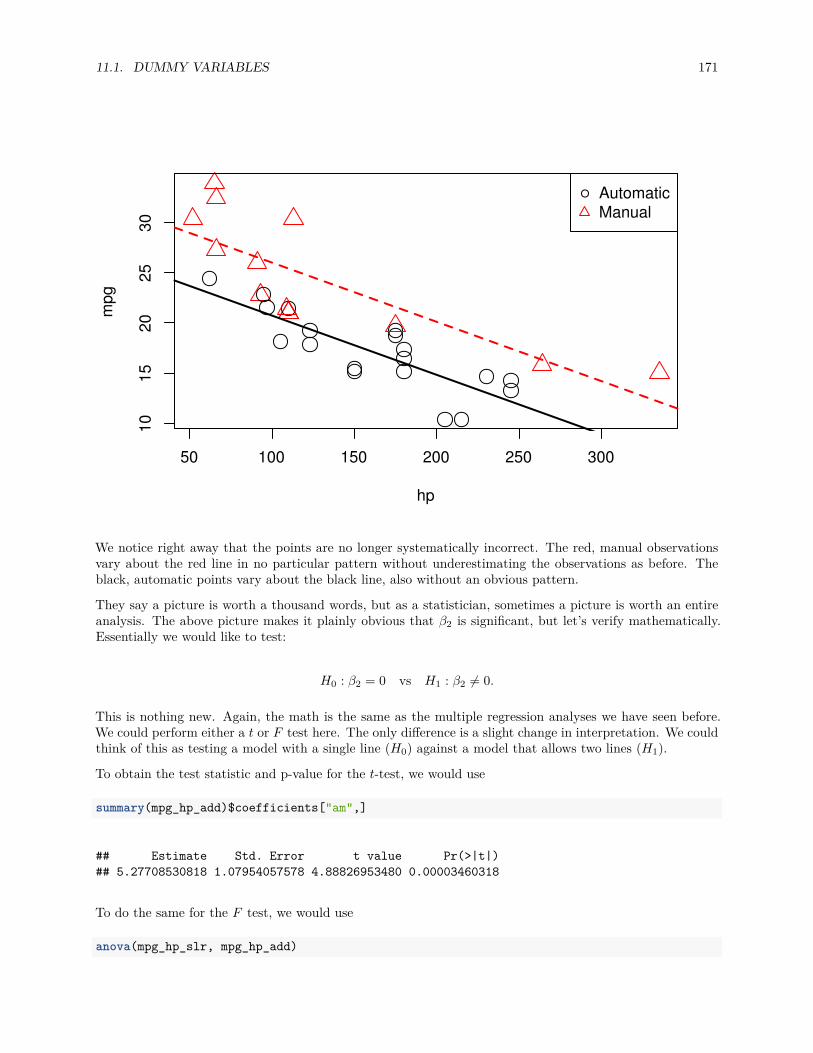
11.1. DUMMY VARIABLES 171
50 100 150 200 250 300
1015
2025
30
hp
mpg
AutomaticManual
We notice right away that the points are no longer systematically incorrect. The red, manual observationsvary about the red line in no particular pattern without underestimating the observations as before. Theblack, automatic points vary about the black line, also without an obvious pattern.
They say a picture is worth a thousand words, but as a statistician, sometimes a picture is worth an entireanalysis. The above picture makes it plainly obvious that β2 is significant, but let’s verify mathematically.Essentially we would like to test:
H0 : β2 = 0 vs H1 : β2 = 0.
This is nothing new. Again, the math is the same as the multiple regression analyses we have seen before.We could perform either a t or F test here. The only difference is a slight change in interpretation. We couldthink of this as testing a model with a single line (H0) against a model that allows two lines (H1).
To obtain the test statistic and p-value for the t-test, we would use
summary(mpg_hp_add)$coefficients["am",]
## Estimate Std. Error t value Pr(>|t|)## 5.27708530818 1.07954057578 4.88826953480 0.00003460318
To do the same for the F test, we would use
anova(mpg_hp_slr, mpg_hp_add)

172 CHAPTER 11. CATEGORICAL PREDICTORS AND INTERACTIONS
## Analysis of Variance Table#### Model 1: mpg ~ hp## Model 2: mpg ~ hp + am## Res.Df RSS Df Sum of Sq F Pr(>F)## 1 30 447.67## 2 29 245.44 1 202.24 23.895 0.0000346 ***## ---## Signif. codes: 0 '***' 0.001 '**' 0.01 '*' 0.05 '.' 0.1 ' ' 1
Notice that these are indeed testing the same thing, as the p-values are exactly equal. (And the F teststatistic is the t test statistic squared.)
Recapping some interpretations:
• β0 = 26.5849137 is the estimated average mpg for a car with an automatic transmission and 0 hp.
• β0 + β2 = 31.8619991 is the estimated average mpg for a car with a manual transmission and 0 hp.
• β2 = 5.2770853 is the estimated difference in average mpg for cars with manual transmissions ascompared to those with automatic transmission, for any hp.
• β1 = −0.0588878 is the estimated change in average mpg for an increase in one hp, for either trans-mission types.
We should take special notice of those last two. In the model,
Y = β0 + β1x1 + β2x2 + ϵ,
we see β1 is the average change in Y for an increase in x1, no matter the value of x2. Also, β2 is always thedifference in the average of Y for any value of x1. These are two restrictions we won’t always want, so weneed a way to specify a more flexible model.
Here we restricted ourselves to a single numerical predictor x1 and one dummy variable x2. However, theconcept of a dummy variable can be used with larger multiple regression models. We only use a singlenumerical predictor here for ease of visualization since we can think of the “two lines” interpretation. Butin general, we can think of a dummy variable as creating “two models,” one for each category of a binarycategorical variable.
11.2 Interactions
To remove the “same slope” restriction, we will now discuss interaction. To illustrate this concept, we willreturn to the autompg dataset we created in the last chapter, with a few more modifications.
# read data frame from the webautompg = read.table("http://archive.ics.uci.edu/ml/machine-learning-databases/auto-mpg/auto-mpg.data",quote = "\"",comment.char = "",stringsAsFactors = FALSE)
# give the dataframe headerscolnames(autompg) = c("mpg", "cyl", "disp", "hp", "wt", "acc", "year", "origin", "name")# remove missing data, which is stored as "?"

11.2. INTERACTIONS 173
autompg = subset(autompg, autompg$hp != "?")# remove the plymouth reliant, as it causes some issuesautompg = subset(autompg, autompg$name != "plymouth reliant")# give the dataset row names, based on the engine, year and namerownames(autompg) = paste(autompg$cyl, "cylinder", autompg$year, autompg$name)# remove the variable for nameautompg = subset(autompg, select = c("mpg", "cyl", "disp", "hp", "wt", "acc", "year", "origin"))# change horsepower from character to numericautompg$hp = as.numeric(autompg$hp)# create a dummary variable for foreign vs domestic cars. domestic = 1.autompg$domestic = as.numeric(autompg$origin == 1)# remove 3 and 5 cylinder cars (which are very rare.)autompg = autompg[autompg$cyl != 5,]autompg = autompg[autompg$cyl != 3,]# the following line would verify the remaining cylinder possibilities are 4, 6, 8#unique(autompg$cyl)# change cyl to a factor variableautompg$cyl = as.factor(autompg$cyl)
str(autompg)
## 'data.frame': 383 obs. of 9 variables:## $ mpg : num 18 15 18 16 17 15 14 14 14 15 ...## $ cyl : Factor w/ 3 levels "4","6","8": 3 3 3 3 3 3 3 3 3 3 ...## $ disp : num 307 350 318 304 302 429 454 440 455 390 ...## $ hp : num 130 165 150 150 140 198 220 215 225 190 ...## $ wt : num 3504 3693 3436 3433 3449 ...## $ acc : num 12 11.5 11 12 10.5 10 9 8.5 10 8.5 ...## $ year : int 70 70 70 70 70 70 70 70 70 70 ...## $ origin : int 1 1 1 1 1 1 1 1 1 1 ...## $ domestic: num 1 1 1 1 1 1 1 1 1 1 ...
We’ve removed cars with 3 and 5 cylinders , as well as created a new variable domestic which indicateswhether or not a car was built in the United States. Removing the 3 and 5 cylinders is simply for ease ofdemonstration later in the chapter and would not be done in practice. The new variable domestic takes thevalue 1 if the car was built in the United States, and 0 otherwise, which we will refer to as “foreign.” (Weare arbitrarily using the United States as the reference point here.) We have also made cyl and origin intofactor variables, which we will discuss later.We’ll now be concerned with three variables: mpg, disp, and domestic. We will use mpg as the response.We can fit a model,
Y = β0 + β1x1 + β2x2 + ϵ,
where
• Y is mpg, the fuel efficiency in miles per gallon,• x1 is disp, the displacement in cubic inches,• x2 is domestic as described above, which is a dummy variable.
x2 =
{1 Domestic0 Foreign
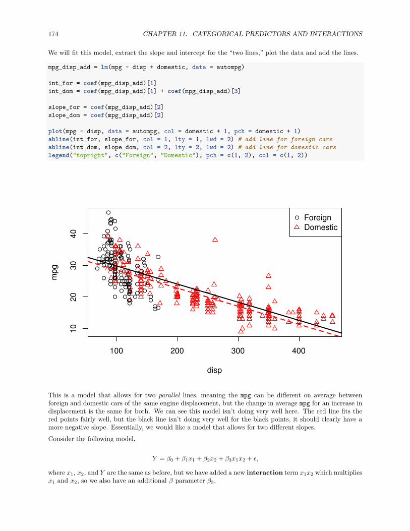
174 CHAPTER 11. CATEGORICAL PREDICTORS AND INTERACTIONS
We will fit this model, extract the slope and intercept for the “two lines,” plot the data and add the lines.
mpg_disp_add = lm(mpg ~ disp + domestic, data = autompg)
int_for = coef(mpg_disp_add)[1]int_dom = coef(mpg_disp_add)[1] + coef(mpg_disp_add)[3]
slope_for = coef(mpg_disp_add)[2]slope_dom = coef(mpg_disp_add)[2]
plot(mpg ~ disp, data = autompg, col = domestic + 1, pch = domestic + 1)abline(int_for, slope_for, col = 1, lty = 1, lwd = 2) # add line for foreign carsabline(int_dom, slope_dom, col = 2, lty = 2, lwd = 2) # add line for domestic carslegend("topright", c("Foreign", "Domestic"), pch = c(1, 2), col = c(1, 2))
100 200 300 400
1020
3040
disp
mpg
ForeignDomestic
This is a model that allows for two parallel lines, meaning the mpg can be different on average betweenforeign and domestic cars of the same engine displacement, but the change in average mpg for an increase indisplacement is the same for both. We can see this model isn’t doing very well here. The red line fits thered points fairly well, but the black line isn’t doing very well for the black points, it should clearly have amore negative slope. Essentially, we would like a model that allows for two different slopes.Consider the following model,
Y = β0 + β1x1 + β2x2 + β3x1x2 + ϵ,
where x1, x2, and Y are the same as before, but we have added a new interaction term x1x2 which multipliesx1 and x2, so we also have an additional β parameter β3.

11.2. INTERACTIONS 175
This model essentially creates two slopes and two intercepts, β2 being the difference in intercepts and β3being the difference in slopes. To see this, we will break down the model into the two “sub-models” forforeign and domestic cars.For foreign cars, that is x2 = 0, we have
Y = β0 + β1x1 + ϵ.
For domestic cars, that is x2 = 1, we have
Y = (β0 + β2) + (β1 + β3)x1 + ϵ.
These two models have both different slopes and intercepts.
• β0 is the average mpg for a foreign car with 0 disp.• β1 is the change in average mpg for an increase of one disp, for foreign cars.• β0 + β2 is the average mpg for a domestic car with 0 disp.• β1 + β3 is the change in average mpg for an increase of one disp, for domestic cars.
How do we fit this model in R? There are a number of ways.One method would be to simply create a new variable, then fit a model like any other.
autompg$x3 = autompg$disp * autompg$domestic # THIS CODE NOT RUN!do_not_do_this = lm(mpg ~ disp + domestic + x3, data = autompg) # THIS CODE NOT RUN!
You should only do this as a last resort. We greatly prefer not to have to modify our data simply to fit amodel. Instead, we can tell R we would like to use the existing data with an interaction term, which it willcreate automatically when we use the : operator.
mpg_disp_int = lm(mpg ~ disp + domestic + disp:domestic, data = autompg)
An alternative method, which will fit the exact same model as above would be to use the * operator. Thismethod automatically creates the interaction term, as well as any “lower order terms,” which in this caseare the first order terms for disp and domestic
mpg_disp_int2 = lm(mpg ~ disp * domestic, data = autompg)
We can quickly verify that these are doing the same thing.
coef(mpg_disp_int)
## (Intercept) disp domestic disp:domestic## 46.0548423 -0.1569239 -12.5754714 0.1025184
coef(mpg_disp_int2)
## (Intercept) disp domestic disp:domestic## 46.0548423 -0.1569239 -12.5754714 0.1025184
We see that both the variables, and their coefficient estimates are indeed the same for both models.
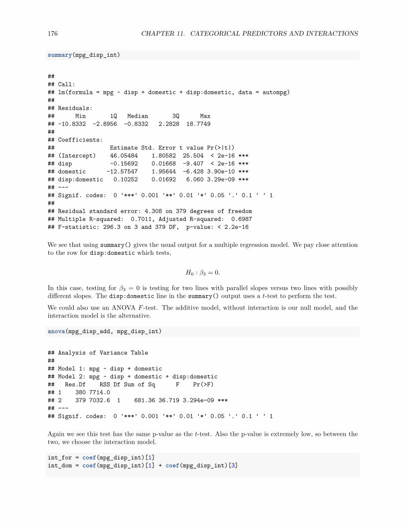
176 CHAPTER 11. CATEGORICAL PREDICTORS AND INTERACTIONS
summary(mpg_disp_int)
#### Call:## lm(formula = mpg ~ disp + domestic + disp:domestic, data = autompg)#### Residuals:## Min 1Q Median 3Q Max## -10.8332 -2.8956 -0.8332 2.2828 18.7749#### Coefficients:## Estimate Std. Error t value Pr(>|t|)## (Intercept) 46.05484 1.80582 25.504 < 2e-16 ***## disp -0.15692 0.01668 -9.407 < 2e-16 ***## domestic -12.57547 1.95644 -6.428 3.90e-10 ***## disp:domestic 0.10252 0.01692 6.060 3.29e-09 ***## ---## Signif. codes: 0 '***' 0.001 '**' 0.01 '*' 0.05 '.' 0.1 ' ' 1#### Residual standard error: 4.308 on 379 degrees of freedom## Multiple R-squared: 0.7011, Adjusted R-squared: 0.6987## F-statistic: 296.3 on 3 and 379 DF, p-value: < 2.2e-16
We see that using summary() gives the usual output for a multiple regression model. We pay close attentionto the row for disp:domestic which tests,
H0 : β3 = 0.
In this case, testing for β3 = 0 is testing for two lines with parallel slopes versus two lines with possiblydifferent slopes. The disp:domestic line in the summary() output uses a t-test to perform the test.
We could also use an ANOVA F -test. The additive model, without interaction is our null model, and theinteraction model is the alternative.
anova(mpg_disp_add, mpg_disp_int)
## Analysis of Variance Table#### Model 1: mpg ~ disp + domestic## Model 2: mpg ~ disp + domestic + disp:domestic## Res.Df RSS Df Sum of Sq F Pr(>F)## 1 380 7714.0## 2 379 7032.6 1 681.36 36.719 3.294e-09 ***## ---## Signif. codes: 0 '***' 0.001 '**' 0.01 '*' 0.05 '.' 0.1 ' ' 1
Again we see this test has the same p-value as the t-test. Also the p-value is extremely low, so between thetwo, we choose the interaction model.
int_for = coef(mpg_disp_int)[1]int_dom = coef(mpg_disp_int)[1] + coef(mpg_disp_int)[3]
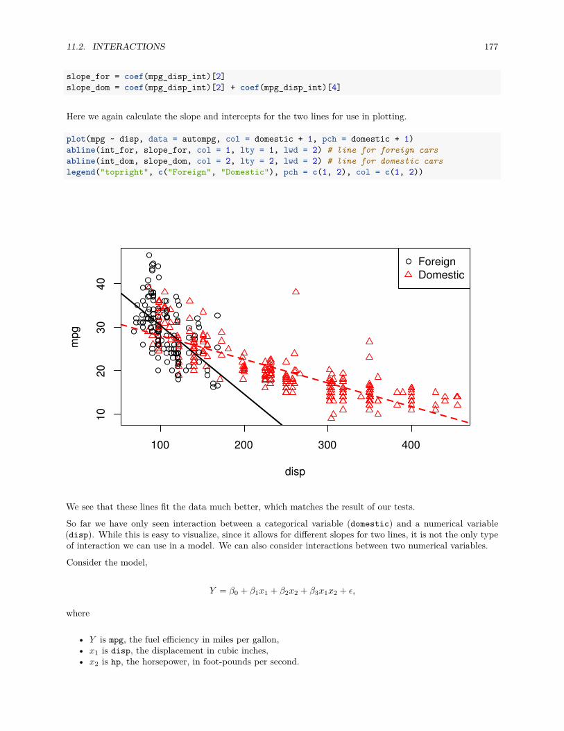
11.2. INTERACTIONS 177
slope_for = coef(mpg_disp_int)[2]slope_dom = coef(mpg_disp_int)[2] + coef(mpg_disp_int)[4]
Here we again calculate the slope and intercepts for the two lines for use in plotting.
plot(mpg ~ disp, data = autompg, col = domestic + 1, pch = domestic + 1)abline(int_for, slope_for, col = 1, lty = 1, lwd = 2) # line for foreign carsabline(int_dom, slope_dom, col = 2, lty = 2, lwd = 2) # line for domestic carslegend("topright", c("Foreign", "Domestic"), pch = c(1, 2), col = c(1, 2))
100 200 300 400
1020
3040
disp
mpg
ForeignDomestic
We see that these lines fit the data much better, which matches the result of our tests.
So far we have only seen interaction between a categorical variable (domestic) and a numerical variable(disp). While this is easy to visualize, since it allows for different slopes for two lines, it is not the only typeof interaction we can use in a model. We can also consider interactions between two numerical variables.
Consider the model,
Y = β0 + β1x1 + β2x2 + β3x1x2 + ϵ,
where
• Y is mpg, the fuel efficiency in miles per gallon,• x1 is disp, the displacement in cubic inches,• x2 is hp, the horsepower, in foot-pounds per second.
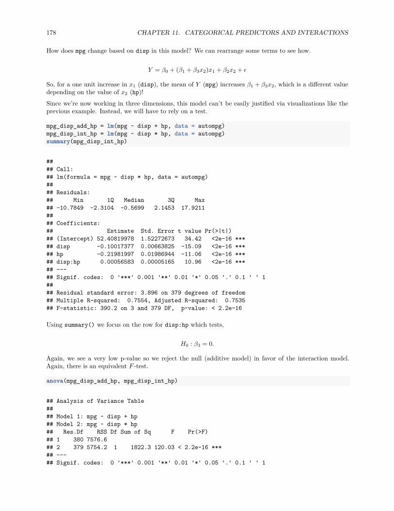
178 CHAPTER 11. CATEGORICAL PREDICTORS AND INTERACTIONS
How does mpg change based on disp in this model? We can rearrange some terms to see how.
Y = β0 + (β1 + β3x2)x1 + β2x2 + ϵ
So, for a one unit increase in x1 (disp), the mean of Y (mpg) increases β1 + β3x2, which is a different valuedepending on the value of x2 (hp)!Since we’re now working in three dimensions, this model can’t be easily justified via visualizations like theprevious example. Instead, we will have to rely on a test.
mpg_disp_add_hp = lm(mpg ~ disp + hp, data = autompg)mpg_disp_int_hp = lm(mpg ~ disp * hp, data = autompg)summary(mpg_disp_int_hp)
#### Call:## lm(formula = mpg ~ disp * hp, data = autompg)#### Residuals:## Min 1Q Median 3Q Max## -10.7849 -2.3104 -0.5699 2.1453 17.9211#### Coefficients:## Estimate Std. Error t value Pr(>|t|)## (Intercept) 52.40819978 1.52272673 34.42 <2e-16 ***## disp -0.10017377 0.00663825 -15.09 <2e-16 ***## hp -0.21981997 0.01986944 -11.06 <2e-16 ***## disp:hp 0.00056583 0.00005165 10.96 <2e-16 ***## ---## Signif. codes: 0 '***' 0.001 '**' 0.01 '*' 0.05 '.' 0.1 ' ' 1#### Residual standard error: 3.896 on 379 degrees of freedom## Multiple R-squared: 0.7554, Adjusted R-squared: 0.7535## F-statistic: 390.2 on 3 and 379 DF, p-value: < 2.2e-16
Using summary() we focus on the row for disp:hp which tests,
H0 : β3 = 0.
Again, we see a very low p-value so we reject the null (additive model) in favor of the interaction model.Again, there is an equivalent F -test.
anova(mpg_disp_add_hp, mpg_disp_int_hp)
## Analysis of Variance Table#### Model 1: mpg ~ disp + hp## Model 2: mpg ~ disp * hp## Res.Df RSS Df Sum of Sq F Pr(>F)## 1 380 7576.6## 2 379 5754.2 1 1822.3 120.03 < 2.2e-16 ***## ---## Signif. codes: 0 '***' 0.001 '**' 0.01 '*' 0.05 '.' 0.1 ' ' 1
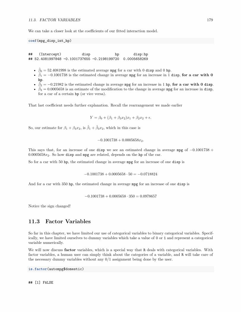
11.3. FACTOR VARIABLES 179
We can take a closer look at the coefficients of our fitted interaction model.
coef(mpg_disp_int_hp)
## (Intercept) disp hp disp:hp## 52.4081997848 -0.1001737655 -0.2198199720 0.0005658269
• β0 = 52.4081998 is the estimated average mpg for a car with 0 disp and 0 hp.• β1 = −0.1001738 is the estimated change in average mpg for an increase in 1 disp, for a car with 0
hp.• β2 = −0.21982 is the estimated change in average mpg for an increase in 1 hp, for a car with 0 disp.• β3 = 0.0005658 is an estimate of the modification to the change in average mpg for an increase in disp,
for a car of a certain hp (or vice versa).
That last coefficient needs further explanation. Recall the rearrangement we made earlier
Y = β0 + (β1 + β3x2)x1 + β2x2 + ϵ.
So, our estimate for β1 + β3x2, is β1 + β3x2, which in this case is
−0.1001738 + 0.0005658x2.
This says that, for an increase of one disp we see an estimated change in average mpg of −0.1001738 +0.0005658x2. So how disp and mpg are related, depends on the hp of the car.
So for a car with 50 hp, the estimated change in average mpg for an increase of one disp is
−0.1001738 + 0.0005658 · 50 = −0.0718824
And for a car with 350 hp, the estimated change in average mpg for an increase of one disp is
−0.1001738 + 0.0005658 · 350 = 0.0978657
Notice the sign changed!
11.3 Factor Variables
So far in this chapter, we have limited our use of categorical variables to binary categorical variables. Specif-ically, we have limited ourselves to dummy variables which take a value of 0 or 1 and represent a categoricalvariable numerically.
We will now discuss factor variables, which is a special way that R deals with categorical variables. Withfactor variables, a human user can simply think about the categories of a variable, and R will take care ofthe necessary dummy variables without any 0/1 assignment being done by the user.
is.factor(autompg$domestic)
## [1] FALSE

180 CHAPTER 11. CATEGORICAL PREDICTORS AND INTERACTIONS
Earlier when we used the domestic variable, it was not a factor variable. It was simply a numerical variablethat only took two possible values, 1 for domestic, and 0 for foreign. Let’s create a new variable origin thatstores the same information, but in a different way.
autompg$origin[autompg$domestic == 1] = "domestic"autompg$origin[autompg$domestic == 0] = "foreign"head(autompg$origin)
## [1] "domestic" "domestic" "domestic" "domestic" "domestic" "domestic"
Now the origin variable stores "domestic" for domestic cars and "foreign" for foreign cars.
is.factor(autompg$origin)
## [1] FALSE
However, this is simply a vector of character values. A vector of car models is a character variable in R. Avector of Vehicle Identification Numbers (VINs) is a character variable as well. But those don’t represent ashort list of levels that might influence a response variable. We will want to coerce this origin variable tobe something more: a factor variable.
autompg$origin = as.factor(autompg$origin)
Now when we check the structure of the autompg dataset, we see that origin is a factor variable.
str(autompg)
## 'data.frame': 383 obs. of 9 variables:## $ mpg : num 18 15 18 16 17 15 14 14 14 15 ...## $ cyl : Factor w/ 3 levels "4","6","8": 3 3 3 3 3 3 3 3 3 3 ...## $ disp : num 307 350 318 304 302 429 454 440 455 390 ...## $ hp : num 130 165 150 150 140 198 220 215 225 190 ...## $ wt : num 3504 3693 3436 3433 3449 ...## $ acc : num 12 11.5 11 12 10.5 10 9 8.5 10 8.5 ...## $ year : int 70 70 70 70 70 70 70 70 70 70 ...## $ origin : Factor w/ 2 levels "domestic","foreign": 1 1 1 1 1 1 1 1 1 1 ...## $ domestic: num 1 1 1 1 1 1 1 1 1 1 ...
Factor variables have levels which are the possible values (categories) that the variable may take, in thiscase foreign or domestic.
levels(autompg$origin)
## [1] "domestic" "foreign"
Recall that previously we have fit the model
Y = β0 + β1x1 + β2x2 + β3x1x2 + ϵ,
where
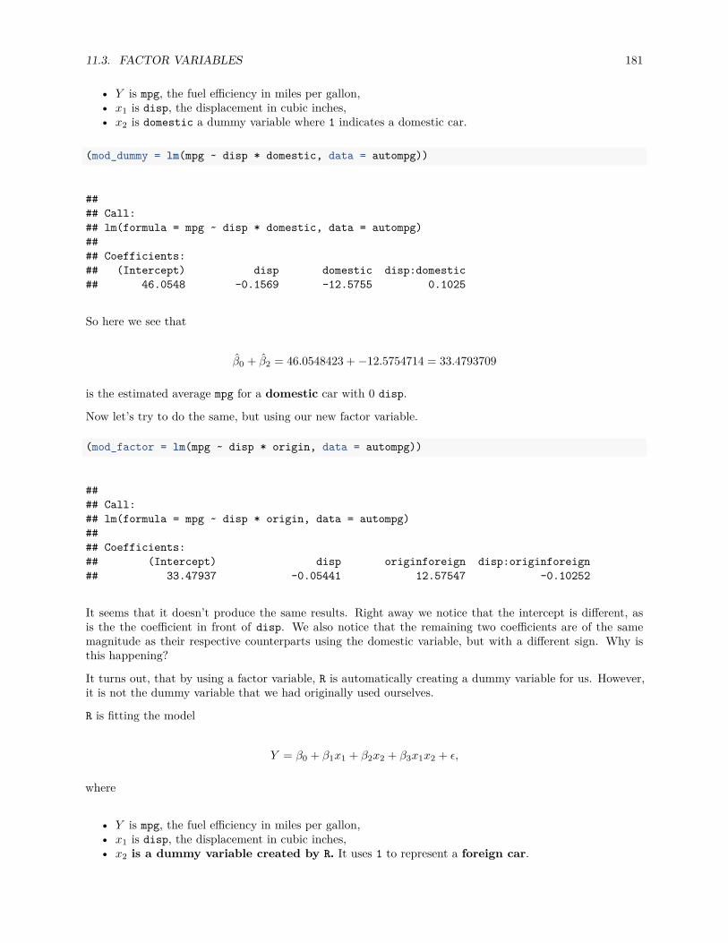
11.3. FACTOR VARIABLES 181
• Y is mpg, the fuel efficiency in miles per gallon,• x1 is disp, the displacement in cubic inches,• x2 is domestic a dummy variable where 1 indicates a domestic car.
(mod_dummy = lm(mpg ~ disp * domestic, data = autompg))
#### Call:## lm(formula = mpg ~ disp * domestic, data = autompg)#### Coefficients:## (Intercept) disp domestic disp:domestic## 46.0548 -0.1569 -12.5755 0.1025
So here we see that
β0 + β2 = 46.0548423 + −12.5754714 = 33.4793709
is the estimated average mpg for a domestic car with 0 disp.
Now let’s try to do the same, but using our new factor variable.
(mod_factor = lm(mpg ~ disp * origin, data = autompg))
#### Call:## lm(formula = mpg ~ disp * origin, data = autompg)#### Coefficients:## (Intercept) disp originforeign disp:originforeign## 33.47937 -0.05441 12.57547 -0.10252
It seems that it doesn’t produce the same results. Right away we notice that the intercept is different, asis the the coefficient in front of disp. We also notice that the remaining two coefficients are of the samemagnitude as their respective counterparts using the domestic variable, but with a different sign. Why isthis happening?
It turns out, that by using a factor variable, R is automatically creating a dummy variable for us. However,it is not the dummy variable that we had originally used ourselves.
R is fitting the model
Y = β0 + β1x1 + β2x2 + β3x1x2 + ϵ,
where
• Y is mpg, the fuel efficiency in miles per gallon,• x1 is disp, the displacement in cubic inches,• x2 is a dummy variable created by R. It uses 1 to represent a foreign car.
182 CHAPTER 11. CATEGORICAL PREDICTORS AND INTERACTIONS
So now,
β0 = 33.4793709
is the estimated average mpg for a domestic car with 0 disp, which is indeed the same as before.
When R created x2, the dummy variable, it used domestic cars as the reference level, that is the defaultvalue of the factor variable. So when the dummy variable is 0, the model represents this reference level,which is domestic. (R makes this choice because domestic comes before foreign alphabetically.)
So the two models have different estimated coefficients, but due to the different model representations, theyare actually the same model.
11.3.1 Factors with More Than Two Levels
Let’s now consider a factor variable with more than two levels. In this dataset, cyl is an example.
is.factor(autompg$cyl)
## [1] TRUE
levels(autompg$cyl)
## [1] "4" "6" "8"
Here the cyl variable has three possible levels: 4, 6, and 8. You may wonder, why not simply use cyl as anumerical variable? You certainly could.
However, that would force the difference in average mpg between 4 and 6 cylinders to be the same as thedifference in average mpg between 6 and 8 cylinders. That usually make senses for a continuous variable, butnot for a discrete variable with so few possible values. In the case of this variable, there is no such thing asa 7-cylinder engine or a 6.23-cylinder engine in personal vehicles. For these reasons, we will simply considercyl to be categorical. This is a decision that will commonly need to be made with ordinal variables. Often,with a large number of categories, the decision to treat them as numerical variables is appropriate because,otherwise, a large number of dummy variables are then needed to represent these variables.
Let’s define three dummy variables related to the cyl factor variable.
v1 =
{1 4 cylinder0 not 4 cylinder
v2 =
{1 6 cylinder0 not 6 cylinder
v3 =
{1 8 cylinder0 not 8 cylinder
Now, let’s fit an additive model in R, using mpg as the response, and disp and cyl as predictors. This shouldbe a model that uses “three regression lines” to model mpg, one for each of the possible cyl levels. They willall have the same slope (since it is an additive model), but each will have its own intercept.

11.3. FACTOR VARIABLES 183
(mpg_disp_add_cyl = lm(mpg ~ disp + cyl, data = autompg))
#### Call:## lm(formula = mpg ~ disp + cyl, data = autompg)#### Coefficients:## (Intercept) disp cyl6 cyl8## 34.99929 -0.05217 -3.63325 -2.03603
The question is, what is the model that R has fit here? It has chosen to use the model
Y = β0 + β1x + β2v2 + β3v3 + ϵ,
where
• Y is mpg, the fuel efficiency in miles per gallon,• x is disp, the displacement in cubic inches,• v2 and v3 are the dummy variables define above.
Why doesn’t R use v1? Essentially because it doesn’t need to. To create three lines, it only needs two dummyvariables since it is using a reference level, which in this case is a 4 cylinder car. The three “sub models” arethen:
• 4 Cylinder: Y = β0 + β1x + ϵ• 6 Cylinder: Y = (β0 + β2) + β1x + ϵ• 8 Cylinder: Y = (β0 + β3) + β1x + ϵ
Notice that they all have the same slope. However, using the two dummy variables, we achieve the threeintercepts.
• β0 is the average mpg for a 4 cylinder car with 0 disp.• β0 + β2 is the average mpg for a 6 cylinder car with 0 disp.• β0 + β3 is the average mpg for a 8 cylinder car with 0 disp.
So because 4 cylinder is the reference level, β0 is specific to 4 cylinders, but β2 and β3 are used to representquantities relative to 4 cylinders.As we have done before, we can extract these intercepts and slopes for the three lines, and plot themaccordingly.
int_4cyl = coef(mpg_disp_add_cyl)[1]int_6cyl = coef(mpg_disp_add_cyl)[1] + coef(mpg_disp_add_cyl)[3]int_8cyl = coef(mpg_disp_add_cyl)[1] + coef(mpg_disp_add_cyl)[4]
slope_all_cyl = coef(mpg_disp_add_cyl)[2]
plot_colors = c("Darkorange", "Darkgrey", "Dodgerblue")plot(mpg ~ disp, data = autompg, col = plot_colors[cyl], pch = as.numeric(cyl))abline(int_4cyl, slope_all_cyl, col = plot_colors[1], lty = 1, lwd = 2)abline(int_6cyl, slope_all_cyl, col = plot_colors[2], lty = 2, lwd = 2)abline(int_8cyl, slope_all_cyl, col = plot_colors[3], lty = 3, lwd = 2)legend("topright", c("4 Cylinder", "6 Cylinder", "8 Cylinder"),
col = plot_colors, lty = c(1, 2, 3), pch = c(1, 2, 3))
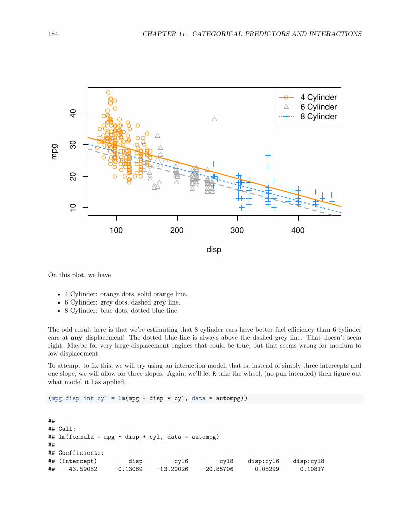
184 CHAPTER 11. CATEGORICAL PREDICTORS AND INTERACTIONS
100 200 300 400
1020
3040
disp
mpg
4 Cylinder6 Cylinder8 Cylinder
On this plot, we have
• 4 Cylinder: orange dots, solid orange line.• 6 Cylinder: grey dots, dashed grey line.• 8 Cylinder: blue dots, dotted blue line.
The odd result here is that we’re estimating that 8 cylinder cars have better fuel efficiency than 6 cylindercars at any displacement! The dotted blue line is always above the dashed grey line. That doesn’t seemright. Maybe for very large displacement engines that could be true, but that seems wrong for medium tolow displacement.
To attempt to fix this, we will try using an interaction model, that is, instead of simply three intercepts andone slope, we will allow for three slopes. Again, we’ll let R take the wheel, (no pun intended) then figure outwhat model it has applied.
(mpg_disp_int_cyl = lm(mpg ~ disp * cyl, data = autompg))
#### Call:## lm(formula = mpg ~ disp * cyl, data = autompg)#### Coefficients:## (Intercept) disp cyl6 cyl8 disp:cyl6 disp:cyl8## 43.59052 -0.13069 -13.20026 -20.85706 0.08299 0.10817

11.3. FACTOR VARIABLES 185
# could also use mpg ~ disp + cyl + disp:cyl
R has again chosen to use 4 cylinder cars as the reference level, but this also now has an effect on theinteraction terms. R has fit the model.
Y = β0 + β1x + β2v2 + β3v3 + γ2xv2 + γ3xv3 + ϵ
We’re using γ like a β parameter for simplicity, so that, for example β2 and γ2 are both associated with v2.
Now, the three “sub models” are:
• 4 Cylinder: Y = β0 + β1x + ϵ.• 6 Cylinder: Y = (β0 + β2) + (β1 + γ2)x + ϵ.• 8 Cylinder: Y = (β0 + β3) + (β1 + γ3)x + ϵ.
Interpreting some parameters and coefficients then:
• (β0 + β2) is the average mpg of a 6 cylinder car with 0 disp• (β1 + γ3) = −0.1306935 + 0.1081714 = −0.0225221 is the estimated change in average mpg for an
increase of one disp, for an 8 cylinder car.
So, as we have seen before β2 and β3 change the intercepts for 6 and 8 cylinder cars relative to the referencelevel of β0 for 4 cylinder cars.
Now, similarly γ2 and γ3 change the slopes for 6 and 8 cylinder cars relative to the reference level of β1 for4 cylinder cars.
Once again, we extract the coefficients and plot the results.
int_4cyl = coef(mpg_disp_int_cyl)[1]int_6cyl = coef(mpg_disp_int_cyl)[1] + coef(mpg_disp_int_cyl)[3]int_8cyl = coef(mpg_disp_int_cyl)[1] + coef(mpg_disp_int_cyl)[4]
slope_4cyl = coef(mpg_disp_int_cyl)[2]slope_6cyl = coef(mpg_disp_int_cyl)[2] + coef(mpg_disp_int_cyl)[5]slope_8cyl = coef(mpg_disp_int_cyl)[2] + coef(mpg_disp_int_cyl)[6]
plot_colors = c("Darkorange", "Darkgrey", "Dodgerblue")plot(mpg ~ disp, data = autompg, col = plot_colors[cyl], pch = as.numeric(cyl))abline(int_4cyl, slope_4cyl, col = plot_colors[1], lty = 1, lwd = 2)abline(int_6cyl, slope_6cyl, col = plot_colors[2], lty = 2, lwd = 2)abline(int_8cyl, slope_8cyl, col = plot_colors[3], lty = 3, lwd = 2)legend("topright", c("4 Cylinder", "6 Cylinder", "8 Cylinder"),
col = plot_colors, lty = c(1, 2, 3), pch = c(1, 2, 3))
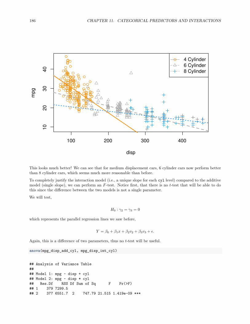
186 CHAPTER 11. CATEGORICAL PREDICTORS AND INTERACTIONS
100 200 300 400
1020
3040
disp
mpg
4 Cylinder6 Cylinder8 Cylinder
This looks much better! We can see that for medium displacement cars, 6 cylinder cars now perform betterthan 8 cylinder cars, which seems much more reasonable than before.
To completely justify the interaction model (i.e., a unique slope for each cyl level) compared to the additivemodel (single slope), we can perform an F -test. Notice first, that there is no t-test that will be able to dothis since the difference between the two models is not a single parameter.
We will test,
H0 : γ2 = γ3 = 0
which represents the parallel regression lines we saw before,
Y = β0 + β1x + β2v2 + β3v3 + ϵ.
Again, this is a difference of two parameters, thus no t-test will be useful.
anova(mpg_disp_add_cyl, mpg_disp_int_cyl)
## Analysis of Variance Table#### Model 1: mpg ~ disp + cyl## Model 2: mpg ~ disp * cyl## Res.Df RSS Df Sum of Sq F Pr(>F)## 1 379 7299.5## 2 377 6551.7 2 747.79 21.515 1.419e-09 ***
11.4. PARAMETERIZATION 187
## ---## Signif. codes: 0 '***' 0.001 '**' 0.01 '*' 0.05 '.' 0.1 ' ' 1
As expected, we see a very low p-value, and thus reject the null. We prefer the interaction model over theadditive model.
Recapping a bit:
• Null Model: Y = β0 + β1x + β2v2 + β3v3 + ϵ
– Number of parameters: q = 4
• Full Model: Y = β0 + β1x + β2v2 + β3v3 + γ2xv2 + γ3xv3 + ϵ
– Number of parameters: p = 6
length(coef(mpg_disp_int_cyl)) - length(coef(mpg_disp_add_cyl))
## [1] 2
We see there is a difference of two parameters, which is also displayed in the resulting ANOVA table from R.Notice that the following two values also appear on the ANOVA table.
nrow(autompg) - length(coef(mpg_disp_int_cyl))
## [1] 377
nrow(autompg) - length(coef(mpg_disp_add_cyl))
## [1] 379
11.4 Parameterization
So far we have been simply letting R decide how to create the dummy variables, and thus R has been decidingthe parameterization of the models. To illustrate the ability to use alternative parameterizations, we willrecreate the data, but directly creating the dummy variables ourselves.
new_param_data = data.frame(y = autompg$mpg,x = autompg$disp,v1 = 1 * as.numeric(autompg$cyl == 4),v2 = 1 * as.numeric(autompg$cyl == 6),v3 = 1 * as.numeric(autompg$cyl == 8))
head(new_param_data, 20)
## y x v1 v2 v3## 1 18 307 0 0 1## 2 15 350 0 0 1## 3 18 318 0 0 1## 4 16 304 0 0 1

188 CHAPTER 11. CATEGORICAL PREDICTORS AND INTERACTIONS
## 5 17 302 0 0 1## 6 15 429 0 0 1## 7 14 454 0 0 1## 8 14 440 0 0 1## 9 14 455 0 0 1## 10 15 390 0 0 1## 11 15 383 0 0 1## 12 14 340 0 0 1## 13 15 400 0 0 1## 14 14 455 0 0 1## 15 24 113 1 0 0## 16 22 198 0 1 0## 17 18 199 0 1 0## 18 21 200 0 1 0## 19 27 97 1 0 0## 20 26 97 1 0 0
Now,
• y is mpg• x is disp, the displacement in cubic inches,• v1, v2, and v3 are dummy variables as defined above.
First let’s try to fit an additive model using x as well as the three dummy variables.
lm(y ~ x + v1 + v2 + v3, data = new_param_data)
#### Call:## lm(formula = y ~ x + v1 + v2 + v3, data = new_param_data)#### Coefficients:## (Intercept) x v1 v2 v3## 32.96326 -0.05217 2.03603 -1.59722 NA
What is happening here? Notice that R is essentially ignoring v3, but why? Well, because R uses an intercept,it cannot also use v3. This is because
1 = v1 + v2 + v3
which means that 1, v1, v2, and v3 are linearly dependent. This would make the X⊤X matrix singular, butwe need to be able to invert it to solve the normal equations and obtain β. With the intercept, v1, and v2,R can make the necessary “three intercepts”. So, in this case v3 is the reference level.
If we remove the intercept, then we can directly obtain all “three intercepts” without a reference level.
lm(y ~ 0 + x + v1 + v2 + v3, data = new_param_data)
#### Call:## lm(formula = y ~ 0 + x + v1 + v2 + v3, data = new_param_data)##

11.4. PARAMETERIZATION 189
## Coefficients:## x v1 v2 v3## -0.05217 34.99929 31.36604 32.96326
Here, we are fitting the model
Y = µ1v1 + µ2v2 + µ3v3 + βx + ϵ.
Thus we have:
• 4 Cylinder: Y = µ1 + βx + ϵ• 6 Cylinder: Y = µ2 + βx + ϵ• 8 Cylinder: Y = µ3 + βx + ϵ
We could also do something similar with the interaction model, and give each line an intercept and slope,without the need for a reference level.
lm(y ~ 0 + v1 + v2 + v3 + x:v1 + x:v2 + x:v3, data = new_param_data)
#### Call:## lm(formula = y ~ 0 + v1 + v2 + v3 + x:v1 + x:v2 + x:v3, data = new_param_data)#### Coefficients:## v1 v2 v3 v1:x v2:x v3:x## 43.59052 30.39026 22.73346 -0.13069 -0.04770 -0.02252
Y = µ1v1 + µ2v2 + µ3v3 + β1xv1 + β2xv2 + β3xv3 + ϵ
• 4 Cylinder: Y = µ1 + β1x + ϵ• 6 Cylinder: Y = µ2 + β2x + ϵ• 8 Cylinder: Y = µ3 + β3x + ϵ
Using the original data, we have (at least) three equivalent ways to specify the interaction model with R.
lm(mpg ~ disp * cyl, data = autompg)
#### Call:## lm(formula = mpg ~ disp * cyl, data = autompg)#### Coefficients:## (Intercept) disp cyl6 cyl8 disp:cyl6 disp:cyl8## 43.59052 -0.13069 -13.20026 -20.85706 0.08299 0.10817
lm(mpg ~ 0 + cyl + disp : cyl, data = autompg)
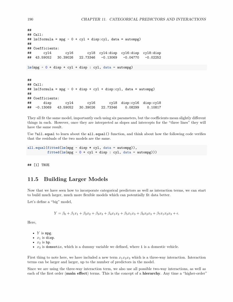
190 CHAPTER 11. CATEGORICAL PREDICTORS AND INTERACTIONS
#### Call:## lm(formula = mpg ~ 0 + cyl + disp:cyl, data = autompg)#### Coefficients:## cyl4 cyl6 cyl8 cyl4:disp cyl6:disp cyl8:disp## 43.59052 30.39026 22.73346 -0.13069 -0.04770 -0.02252
lm(mpg ~ 0 + disp + cyl + disp : cyl, data = autompg)
#### Call:## lm(formula = mpg ~ 0 + disp + cyl + disp:cyl, data = autompg)#### Coefficients:## disp cyl4 cyl6 cyl8 disp:cyl6 disp:cyl8## -0.13069 43.59052 30.39026 22.73346 0.08299 0.10817
They all fit the same model, importantly each using six parameters, but the coefficients mean slightly differentthings in each. However, once they are interpreted as slopes and intercepts for the “three lines” they willhave the same result.
Use ?all.equal to learn about the all.equal() function, and think about how the following code verifiesthat the residuals of the two models are the same.
all.equal(fitted(lm(mpg ~ disp * cyl, data = autompg)),fitted(lm(mpg ~ 0 + cyl + disp : cyl, data = autompg)))
## [1] TRUE
11.5 Building Larger Models
Now that we have seen how to incorporate categorical predictors as well as interaction terms, we can startto build much larger, much more flexible models which can potentially fit data better.
Let’s define a “big” model,
Y = β0 + β1x1 + β2x2 + β3x3 + β4x1x2 + β5x1x3 + β6x2x3 + β7x1x2x3 + ϵ.
Here,
• Y is mpg.• x1 is disp.• x2 is hp.• x3 is domestic, which is a dummy variable we defined, where 1 is a domestic vehicle.
First thing to note here, we have included a new term x1x2x3 which is a three-way interaction. Interactionterms can be larger and larger, up to the number of predictors in the model.
Since we are using the three-way interaction term, we also use all possible two-way interactions, as well aseach of the first order (main effect) terms. This is the concept of a hierarchy. Any time a “higher-order”

11.5. BUILDING LARGER MODELS 191
term is in a model, the related “lower-order” terms should also be included. Mathematically their inclusionor exclusion is sometimes irrelevant, but from an interpretation standpoint, it is best to follow the hierarchyrules.
Let’s do some rearrangement to obtain a “coefficient” in front of x1.
Y = β0 + β2x2 + β3x3 + β6x2x3 + (β1 + β4x2 + β5x3 + β7x2x3)x1 + ϵ.
Specifically, the “coefficient” in front of x1 is
(β1 + β4x2 + β5x3 + β7x2x3).
Let’s discuss this “coefficient” to help us understand the idea of the flexibility of a model. Recall that,
• β1 is the coefficient for a first order term,• β4 and β5 are coefficients for two-way interactions,• β7 is the coefficient for the three-way interaction.
If the two and three way interactions were not in the model, the whole “coefficient” would simply be
β1.
Thus, no matter the values of x2 and x3, β1 would determine the relationship between x1 (disp) and Y(mpg).
With the addition of the two-way interactions, now the “coefficient” would be
(β1 + β4x2 + β5x3).
Now, changing x1 (disp) has a different effect on Y (mpg), depending on the values of x2 and x3.
Lastly, adding the three-way interaction gives the whole “coefficient”
(β1 + β4x2 + β5x3 + β7x2x3)
which is even more flexible. Now changing x1 (disp) has a different effect on Y (mpg), depending on thevalues of x2 and x3, but in a more flexible way which we can see with some more rearrangement. Now the“coefficient” in front of x3 in this “coefficient” is dependent on x2.
(β1 + β4x2 + (β5 + β7x2)x3)
It is so flexible, it is becoming hard to interpret!
Let’s fit this three-way interaction model in R.
big_model = lm(mpg ~ disp * hp * domestic, data = autompg)summary(big_model)

192 CHAPTER 11. CATEGORICAL PREDICTORS AND INTERACTIONS
#### Call:## lm(formula = mpg ~ disp * hp * domestic, data = autompg)#### Residuals:## Min 1Q Median 3Q Max## -11.9410 -2.2147 -0.4008 1.9430 18.4094#### Coefficients:## Estimate Std. Error t value Pr(>|t|)## (Intercept) 60.6457838 6.6000851 9.189 < 2e-16 ***## disp -0.1415870 0.0634395 -2.232 0.0262 *## hp -0.3544717 0.0812261 -4.364 0.0000165 ***## domestic -12.5718884 7.0643505 -1.780 0.0759 .## disp:hp 0.0013690 0.0006727 2.035 0.0426 *## disp:domestic 0.0493298 0.0640046 0.771 0.4414## hp:domestic 0.1851530 0.0870881 2.126 0.0342 *## disp:hp:domestic -0.0009163 0.0006768 -1.354 0.1766## ---## Signif. codes: 0 '***' 0.001 '**' 0.01 '*' 0.05 '.' 0.1 ' ' 1#### Residual standard error: 3.88 on 375 degrees of freedom## Multiple R-squared: 0.76, Adjusted R-squared: 0.7556## F-statistic: 169.7 on 7 and 375 DF, p-value: < 2.2e-16
Do we actually need this large of a model? Let’s first test for the necessity of the three-way interaction term.That is,
H0 : β7 = 0.
So,
• Full Model: Y = β0 + β1x1 + β2x2 + β3x3 + β4x1x2 + β5x1x3 + β6x2x3 + β7x1x2x3 + ϵ• Null Model: Y = β0 + β1x1 + β2x2 + β3x3 + β4x1x2 + β5x1x3 + β6x2x3 + ϵ
We fit the null model in R as two_way_int_mod, then use anova() to perform an F -test as usual.
two_way_int_mod = lm(mpg ~ disp * hp + disp * domestic + hp * domestic, data = autompg)#two_way_int_mod = lm(mpg ~ (disp + hp + domestic) ^ 2, data = autompg)anova(two_way_int_mod, big_model)
## Analysis of Variance Table#### Model 1: mpg ~ disp * hp + disp * domestic + hp * domestic## Model 2: mpg ~ disp * hp * domestic## Res.Df RSS Df Sum of Sq F Pr(>F)## 1 376 5673.2## 2 375 5645.6 1 27.599 1.8332 0.1766
We see the p-value is somewhat large, so we would fail to reject. We prefer the smaller, less flexible, nullmodel, without the three-way interaction.A quick note here: the full model does still “fit better.” Notice that it has a smaller RMSE than the nullmodel, which means the full model makes smaller (squared) errors on average.

11.5. BUILDING LARGER MODELS 193
mean(resid(big_model) ^ 2)
## [1] 14.74053
mean(resid(two_way_int_mod) ^ 2)
## [1] 14.81259
However, it is not much smaller. We could even say that, the difference is insignificant. This is an idea wewill return to later in greater detail.
Now that we have chosen the model without the three-way interaction, can we go further? Do we need thetwo-way interactions? Let’s test
H0 : β4 = β5 = β6 = 0.
Remember we already chose β7 = 0, so,
• Full Model: Y = β0 + β1x1 + β2x2 + β3x3 + β4x1x2 + β5x1x3 + β6x2x3 + ϵ• Null Model: Y = β0 + β1x1 + β2x2 + β3x3 + ϵ
We fit the null model in R as additive_mod, then use anova() to perform an F -test as usual.
additive_mod = lm(mpg ~ disp + hp + domestic, data = autompg)anova(additive_mod, two_way_int_mod)
## Analysis of Variance Table#### Model 1: mpg ~ disp + hp + domestic## Model 2: mpg ~ disp * hp + disp * domestic + hp * domestic## Res.Df RSS Df Sum of Sq F Pr(>F)## 1 379 7369.7## 2 376 5673.2 3 1696.5 37.478 < 2.2e-16 ***## ---## Signif. codes: 0 '***' 0.001 '**' 0.01 '*' 0.05 '.' 0.1 ' ' 1
Here the p-value is small, so we reject the null, and we prefer the full (alternative) model. Of the models wehave considered, our final preference is for
Y = β0 + β1x1 + β2x2 + β3x3 + β4x1x2 + β5x1x3 + β6x2x3 + ϵ.

194 CHAPTER 11. CATEGORICAL PREDICTORS AND INTERACTIONS

Chapter 12
Analysis of Variance
Chapter Status: This chapter should be considered optional for a first reading of this text. Its inclusionis mostly for the benefit of some courses that use the text. Additionally, this chapter is currently somewhatunderdeveloped compared to the rest of the text. If you are interested in contributing, you can find severallines marked “TODO” in the source. Pull requests encouraged!
“To find out what happens when you change something, it is necessary to change it.”— Box, Hunter, and Hunter, Statistics for Experimenters (1978)
Thus far, we have built models for numeric responses, when the predictors are all numeric. We’ll take a minordetour to go back and consider models which only have categorical predictors. A categorical predictor isa variable which takes only a finite number of values, which are not ordered. For example a variable whichtakes possible values red, blue, green is categorical. In the context of using a categorical variable as apredictor, it would place observations into different groups (categories).
We’ve also mostly been dealing with observational data. The methods in this section are most useful inexperimental settings, but still work with observational data. (However, for determining causation, werequire experiments.)
12.1 Experiments
The biggest difference between an observational study and an experiment is how the predictor data isobtained. Is the experimenter in control?
• In an observational study, both response and predictor data are obtained via observation.• In an experiment, the predictor data are values determined by the experimenter. The experiment is
run and the response is observed.
In an experiment, the predictors, which are controlled by the experimenter, are called factors. The possiblevalues of these factors are called levels. Subjects are randomly assigned to a level of each of the factors.
The design of experiments could be a course by itself. The Wikipedia article on design of experiments givesa good overview. Originally, most of the methodology was developed for agricultural applications by R. A.Fisher, but are still in use today, now in a wide variety of application areas. Notably, these methods haveseen a resurgence as a part of “A/B Testing.”
195
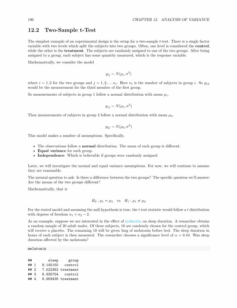
196 CHAPTER 12. ANALYSIS OF VARIANCE
12.2 Two-Sample t-Test
The simplest example of an experimental design is the setup for a two-sample t-test. There is a single factorvariable with two levels which split the subjects into two groups. Often, one level is considered the control,while the other is the treatment. The subjects are randomly assigned to one of the two groups. After beingassigned to a group, each subject has some quantity measured, which is the response variable.
Mathematically, we consider the model
yij ∼ N(µi, σ2)
where i = 1, 2 for the two groups and j = 1, 2, . . . ni. Here ni is the number of subjects in group i. So y13would be the measurement for the third member of the first group.
So measurements of subjects in group 1 follow a normal distribution with mean µ1.
y1j ∼ N(µ1, σ2)
Then measurements of subjects in group 2 follow a normal distribution with mean µ2.
y2j ∼ N(µ2, σ2)
This model makes a number of assumptions. Specifically,
• The observations follow a normal distribution. The mean of each group is different.• Equal variance for each group.• Independence. Which is believable if groups were randomly assigned.
Later, we will investigate the normal and equal variance assumptions. For now, we will continue to assumethey are reasonable.
The natural question to ask: Is there a difference between the two groups? The specific question we’ll answer:Are the means of the two groups different?
Mathematically, that is
H0 : µ1 = µ2 vs H1 : µ1 = µ2
For the stated model and assuming the null hypothesis is true, the t test statistic would follow a t distributionwith degrees of freedom n1 + n2 − 2.
As an example, suppose we are interested in the effect of melatotin on sleep duration. A researcher obtainsa random sample of 20 adult males. Of these subjects, 10 are randomly chosen for the control group, whichwill receive a placebo. The remaining 10 will be given 5mg of melatonin before bed. The sleep duration inhours of each subject is then measured. The researcher chooses a significance level of α = 0.10. Was sleepduration affected by the melatonin?
melatonin
## sleep group## 1 8.145150 control## 2 7.522362 treatment## 3 6.935754 control## 4 8.959435 treatment

12.2. TWO-SAMPLE T-TEST 197
## 5 6.985122 control## 6 8.072651 treatment## 7 8.313826 control## 8 8.086409 treatment## 9 8.922108 control## 10 8.124743 treatment## 11 8.065844 control## 12 10.943974 treatment## 13 4.833367 control## 14 7.865453 treatment## 15 6.340014 control## 16 8.963140 treatment## 17 6.158896 control## 18 5.012253 treatment## 19 3.571440 control## 20 9.784136 treatment
Here, we would like to test,
H0 : µC = µT vs H1 : µC = µT
To do so in R, we use the t.test() function, with the var.equal argument set to TRUE.
t.test(sleep ~ group, data = melatonin, var.equal = TRUE)
#### Two Sample t-test#### data: sleep by group## t = -2.0854, df = 18, p-value = 0.05154## alternative hypothesis: true difference in means is not equal to 0## 95 percent confidence interval:## -3.02378261 0.01117547## sample estimates:## mean in group control mean in group treatment## 6.827152 8.333456
At a significance level of α = 0.10, we reject the null hypothesis. It seems that the melatonin had astatistically significant effect. Be aware that statistical significance is not always the same as scientific orpractical significance. To determine practical significance, we need to investigate the effect size in thecontext of the situation. Here the effect size is the difference of the sample means.
t.test(sleep ~ group, data = melatonin, var.equal = TRUE)$estimate
## mean in group control mean in group treatment## 6.827152 8.333456
Here we see that the subjects in the melatonin group sleep an average of about 1.5 hours longer than thecontrol group. An hour and a half of sleep is certainly important!With a big enough sample size, we could make an effect size of say, four minutes statistically significant. Isit worth taking a pill every night to get an extra four minutes of sleep? (Probably not.)
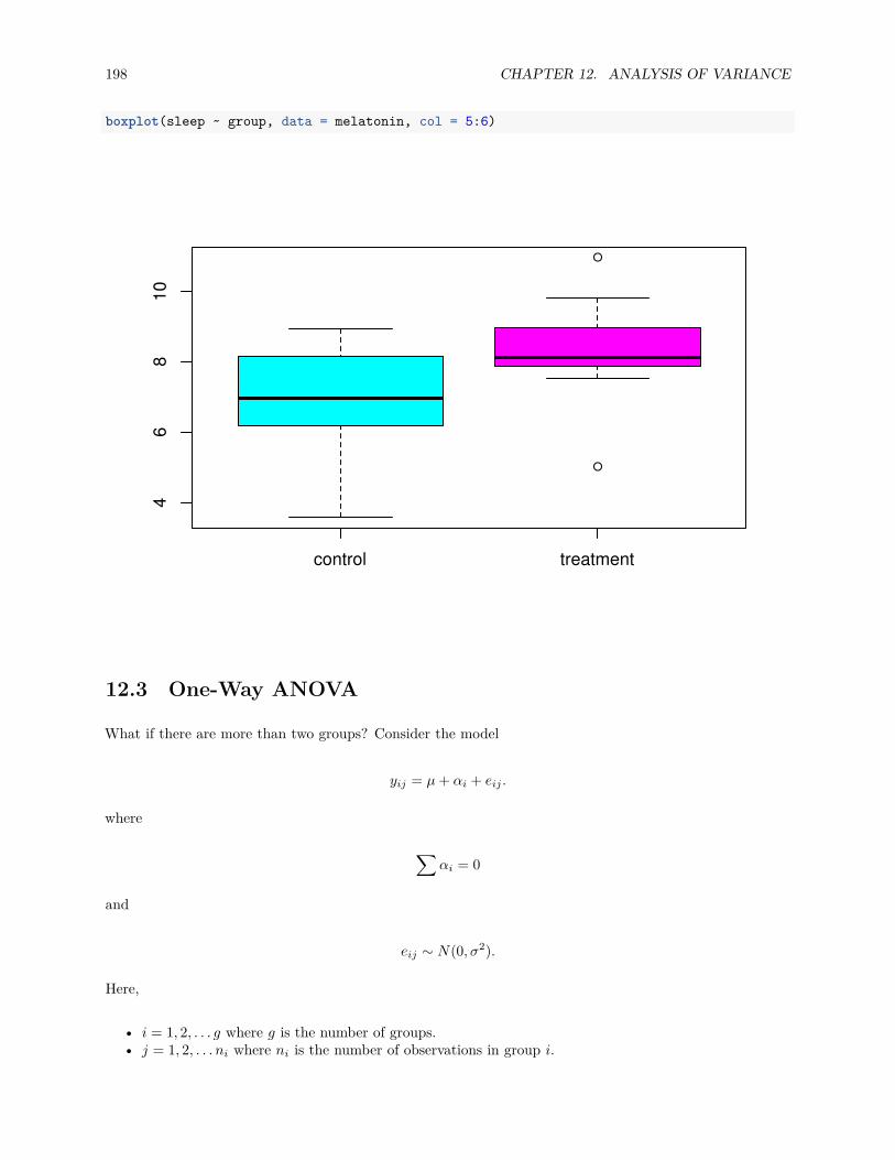
198 CHAPTER 12. ANALYSIS OF VARIANCE
boxplot(sleep ~ group, data = melatonin, col = 5:6)
control treatment
46
810
12.3 One-Way ANOVA
What if there are more than two groups? Consider the model
yij = µ + αi + eij .
where
∑αi = 0
and
eij ∼ N(0, σ2).
Here,
• i = 1, 2, . . . g where g is the number of groups.• j = 1, 2, . . . ni where ni is the number of observations in group i.

12.3. ONE-WAY ANOVA 199
Then the total sample size is
N =g∑
i=i
ni
Observations from group i follow a normal distribution
yij ∼ N(µi, σ2)
where the mean of each group is given by
µi = µ + αi.
Here αi measures the effect of group i. It is the difference between the overall mean and the mean of groupi.
Essentially, the assumptions here are the same as the two sample case, however now, we simply have moregroups.
Much like the two-sample case, we would again like to test if the means of the groups are equal.
H0 : µ1 = µ2 = . . . µg vs H1 : Not all µi are equal.
Notice that the alternative simply indicates the some of the means are not equal, not specifically which arenot equal. More on that later.
Alternatively, we could write
H0 : α1 = α2 = . . . = αg = 0 vs H1 : Not all αi are 0.
This test is called Analysis of Variance. Analysis of Variance (ANOVA) compares the variation due tospecific sources (between groups) with the variation among individuals who should be similar (within groups).In particular, ANOVA tests whether several populations have the same mean by comparing how far apartthe sample means are with how much variation there is within the samples. We use variability of means totest for equality of means, thus the use of variance in the name for a test about means.
We’ll leave out most of the details about how the estimation is done, but we’ll see later, that it is done vialeast squares. We’ll use R to obtain these estimates, but they are actually rather simple. We only need tothink about the sample means of the groups.
• yi is the sample mean of group i.• y is the overall sample mean.• s2
i is the sample variance of group i.
We’ll then decompose the variance, as we’ve seen before in regression. The total variation measures howmuch the observations vary about the overall sample mean, ignoring the groups.
SST =g∑
i=i
ni∑j=1
(yij − y)2
The variation between groups looks at how far the individual sample means are from the overall samplemean.
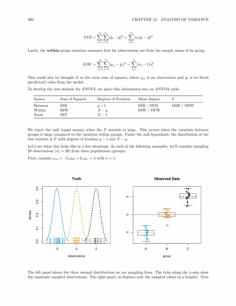
200 CHAPTER 12. ANALYSIS OF VARIANCE
SSB =g∑
i=i
ni∑j=1
(yi − y)2 =g∑
i=i
ni(yi − y)2
Lastly, the within group variation measures how far observations are from the sample mean of its group.
SSW =g∑
i=i
ni∑j=1
(yij − yi)2 =g∑
i=i
(ni − 1)s2i
This could also be thought of as the error sum of squares, where yij is an observation and yi is its fitted(predicted) value from the model.
To develop the test statistic for ANOVA, we place this information into an ANVOA table.
Source Sum of Squares Degrees of Freedom Mean Square F
Between SSB g − 1 SSB / DFB MSB / MSWWithin SSW N − g SSW / DFWTotal SST N − 1
We reject the null (equal means) when the F statistic is large. This occurs when the variation betweengroups is large compared to the variation within groups. Under the null hypothesis, the distribution of thetest statistic is F with degrees of freedom g − 1 and N − g.
Let’s see what this looks like in a few situations. In each of the following examples, we’ll consider sampling20 observations (ni = 20) from three populations (groups).
First, consider µA = −5, µB = 0, µC = 5 with σ = 1.
-5 0 5
0.0
0.1
0.2
0.3
0.4
Truth
observations
dens
ity
A B C
-50
5
Observed Data
group
The left panel shows the three normal distributions we are sampling from. The ticks along the x-axis showthe randomly sampled observations. The right panel, re-displays only the sampled values in a boxplot. Note
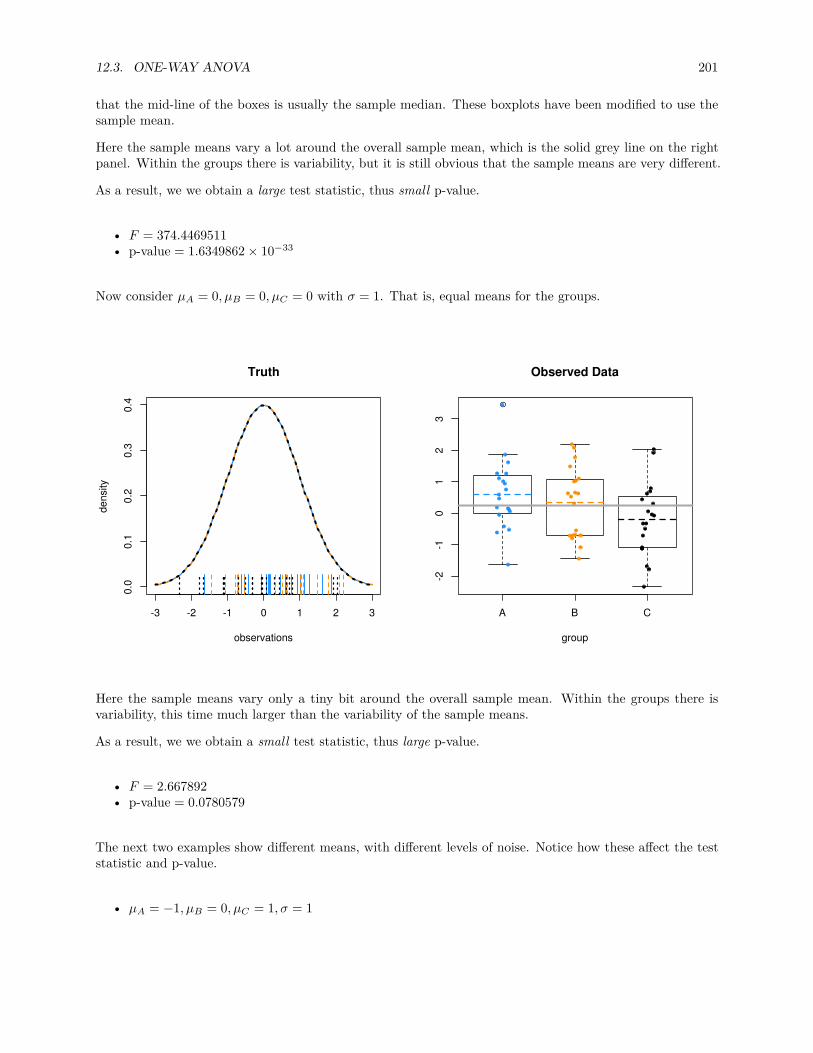
12.3. ONE-WAY ANOVA 201
that the mid-line of the boxes is usually the sample median. These boxplots have been modified to use thesample mean.
Here the sample means vary a lot around the overall sample mean, which is the solid grey line on the rightpanel. Within the groups there is variability, but it is still obvious that the sample means are very different.
As a result, we we obtain a large test statistic, thus small p-value.
• F = 374.4469511• p-value = 1.6349862 × 10⁻³³
Now consider µA = 0, µB = 0, µC = 0 with σ = 1. That is, equal means for the groups.
-3 -2 -1 0 1 2 3
0.0
0.1
0.2
0.3
0.4
Truth
observations
dens
ity
A B C
-2-1
01
23
Observed Data
group
Here the sample means vary only a tiny bit around the overall sample mean. Within the groups there isvariability, this time much larger than the variability of the sample means.
As a result, we we obtain a small test statistic, thus large p-value.
• F = 2.667892• p-value = 0.0780579
The next two examples show different means, with different levels of noise. Notice how these affect the teststatistic and p-value.
• µA = −1, µB = 0, µC = 1, σ = 1
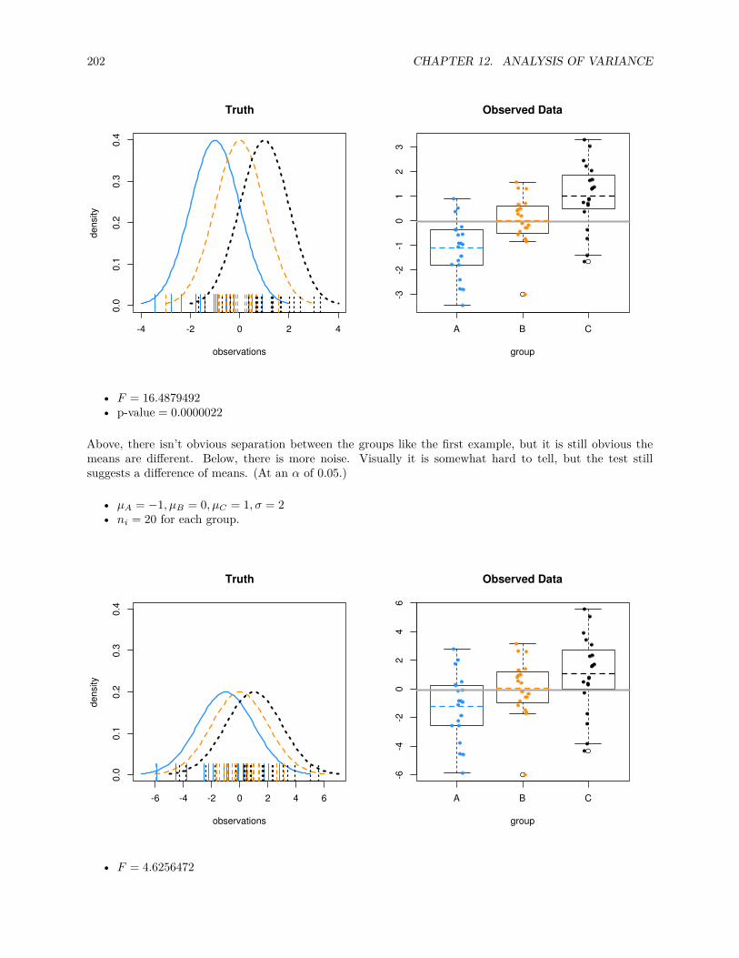
202 CHAPTER 12. ANALYSIS OF VARIANCE
-4 -2 0 2 4
0.0
0.1
0.2
0.3
0.4
Truth
observations
dens
ity
A B C
-3-2
-10
12
3
Observed Data
group
• F = 16.4879492• p-value = 0.0000022
Above, there isn’t obvious separation between the groups like the first example, but it is still obvious themeans are different. Below, there is more noise. Visually it is somewhat hard to tell, but the test stillsuggests a difference of means. (At an α of 0.05.)
• µA = −1, µB = 0, µC = 1, σ = 2• ni = 20 for each group.
-6 -4 -2 0 2 4 6
0.0
0.1
0.2
0.3
0.4
Truth
observations
dens
ity
A B C
-6-4
-20
24
6
Observed Data
group
• F = 4.6256472

12.3. ONE-WAY ANOVA 203
• p-value = 0.0137529
Let’s consider an example with real data. We’ll use the coagulation dataset from the faraway package.Here four different diets (A, B, C, D) were administered to a random sample of 24 animals. The subjects wererandomly assigned to one of the four diets. For each, their blood coagulation time was measured in seconds.
Here we would like to test
H0 : µA = µB = µC = µD
where, for example, µA is the mean blood coagulation time for an animal that ate diet A.
library(faraway)names(coagulation)
## [1] "coag" "diet"
plot(coag ~ diet, data = coagulation, col = 2:5)
A B C D
6065
70
diet
coag
We first load the data and create the relevant boxplot. The plot alone suggests a difference of means. Theaov() function is used to obtain the relevant sums of squares. Using the summary() function on the outputfrom aov() creates the desired ANOVA table. (Without the unneeded row for total.)
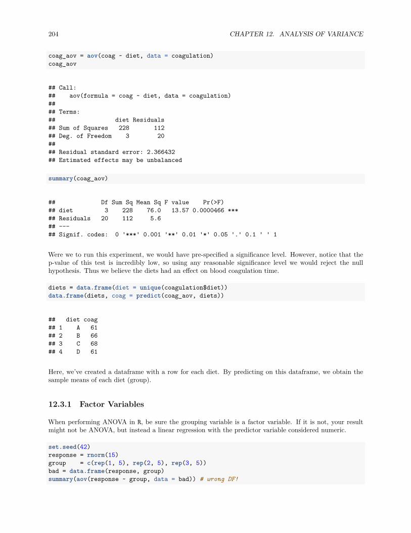
204 CHAPTER 12. ANALYSIS OF VARIANCE
coag_aov = aov(coag ~ diet, data = coagulation)coag_aov
## Call:## aov(formula = coag ~ diet, data = coagulation)#### Terms:## diet Residuals## Sum of Squares 228 112## Deg. of Freedom 3 20#### Residual standard error: 2.366432## Estimated effects may be unbalanced
summary(coag_aov)
## Df Sum Sq Mean Sq F value Pr(>F)## diet 3 228 76.0 13.57 0.0000466 ***## Residuals 20 112 5.6## ---## Signif. codes: 0 '***' 0.001 '**' 0.01 '*' 0.05 '.' 0.1 ' ' 1
Were we to run this experiment, we would have pre-specified a significance level. However, notice that thep-value of this test is incredibly low, so using any reasonable significance level we would reject the nullhypothesis. Thus we believe the diets had an effect on blood coagulation time.
diets = data.frame(diet = unique(coagulation$diet))data.frame(diets, coag = predict(coag_aov, diets))
## diet coag## 1 A 61## 2 B 66## 3 C 68## 4 D 61
Here, we’ve created a dataframe with a row for each diet. By predicting on this dataframe, we obtain thesample means of each diet (group).
12.3.1 Factor Variables
When performing ANOVA in R, be sure the grouping variable is a factor variable. If it is not, your resultmight not be ANOVA, but instead a linear regression with the predictor variable considered numeric.
set.seed(42)response = rnorm(15)group = c(rep(1, 5), rep(2, 5), rep(3, 5))bad = data.frame(response, group)summary(aov(response ~ group, data = bad)) # wrong DF!

12.3. ONE-WAY ANOVA 205
## Df Sum Sq Mean Sq F value Pr(>F)## group 1 0.017 0.0173 0.015 0.903## Residuals 13 14.698 1.1306
good = data.frame(response, group = as.factor(group))summary(aov(response ~ group, data = good))
## Df Sum Sq Mean Sq F value Pr(>F)## group 2 0.232 0.1158 0.096 0.909## Residuals 12 14.484 1.2070
is.factor(bad$group) # 1, 2, and 3 are numbers.
## [1] FALSE
is.factor(good$group) # 1, 2, and 3 are labels.
## [1] TRUE
12.3.2 Some Simulation
Here we verify the distribution of the test statistic under the null hypothesis. We simulate from a null model(equal variance) to obtain an empirical distribution of the F statistic. We add the curve for the expecteddistribution.
library(broom)
sim_anova = function(n = 10, mu_a = 0, mu_b = 0, mu_c = 0, mu_d = 0, sigma = 1, stat = TRUE) {
# create data from one-way ANOVA model with four groups of equal size# response simulated from normal with group mean, shared variance# group variable indicates group A, B, C or Dsim_data = data.frame(response = c(rnorm(n = n, mean = mu_a, sd = sigma),
rnorm(n = n, mean = mu_b, sd = sigma),rnorm(n = n, mean = mu_c, sd = sigma),rnorm(n = n, mean = mu_d, sd = sigma)),
group = c(rep("A", times = n), rep("B", times = n),rep("C", times = n), rep("D", times = n))
)
# obtain F-statistic and p-value for testing difference of meansaov_results = aov(response ~ group, data = sim_data)f_stat = glance(aov_results)$statp_val = glance(aov_results)$p.val
# return f_stat if stat = TRUE, otheriwse, p-valueifelse(stat, f_stat, p_val)
}

206 CHAPTER 12. ANALYSIS OF VARIANCE
f_stats = replicate(n = 5000, sim_anova(stat = TRUE))hist(f_stats, breaks = 100, prob = TRUE, border = "dodgerblue", main = "Empirical Distribution of F")curve(df(x, df1 = 4 - 1, df2 = 40 - 4), col = "darkorange", add = TRUE, lwd = 2)
Empirical Distribution of F
f_stats
Den
sity
0 1 2 3 4 5 6
0.0
0.2
0.4
0.6
12.3.3 Power
Now that we’re performing experiments, getting more data means finding more test subjects, running morelab tests, etc. In other words, it will cost more time and money.
We’d like to design our experiment so that we have a good chance of detecting an interesting effect size,without spending too much money. There’s no point in running an experiment if there’s only a very lowchance that it has a significant result that you care about. (Remember, not all statistically significant resultshave practical value.)
We’d like the ANOVA test to have high power for an alternative hypothesis with a minimum desired effectsize.
Power = P (Rejct H0 | H0 False)
That is, for a true difference of means that we deem interesting, we want the test to reject with highprobability.
A number of things can affect the power of a test:
• Effect size. It is easier to detect larger effects.

12.4. POST HOC TESTING 207
• Noise level σ. The less noise, the easier it is to detect signal (effect). We don’t have much ability tocontrol this, except maybe to measure more accurately.
• Significance level α. Lower significance level makes rejecting more difficult. (But also allows for lessfalse positives.)
• Sample size. Large samples means easier to detect effects.• Balanced design. An equal number of observations per group leads to higher power.
The following simulations look at the effect of significance level, effect size, and noise level on the power ofan ANOVA F -test. Homework will look into sample size and balance.
p_vals = replicate(n = 1000, sim_anova(mu_a = -1, mu_b = 0, mu_c = 0, mu_d = 1,sigma = 1.5, stat = FALSE))
mean(p_vals < 0.05)
## [1] 0.663
mean(p_vals < 0.01)
## [1] 0.39
p_vals = replicate(n = 1000, sim_anova(mu_a = -1, mu_b = 0, mu_c = 0, mu_d = 1,sigma = 2.0, stat = FALSE))
mean(p_vals < 0.05)
## [1] 0.408
mean(p_vals < 0.01)
## [1] 0.179
p_vals = replicate(n = 1000, sim_anova(mu_a = -2, mu_b = 0, mu_c = 0, mu_d = 2,sigma = 2.0, stat = FALSE))
mean(p_vals < 0.05)
## [1] 0.964
mean(p_vals < 0.01)
## [1] 0.855
12.4 Post Hoc Testing
Suppose we reject the null hypothesis from the ANOVA test for equal means. That tells us that the meansare different. But which means? All of them? Some of them? The obvious strategy is to test all possiblecomparisons of two means. We can do this easily in R.

208 CHAPTER 12. ANALYSIS OF VARIANCE
with(coagulation, pairwise.t.test(coag, diet, p.adj = "none"))
#### Pairwise comparisons using t tests with pooled SD#### data: coag and diet#### A B C## B 0.00380 - -## C 0.00018 0.15878 -## D 1.00000 0.00086 0.000023#### P value adjustment method: none
# pairwise.t.test(coagulation$coag, coagulation$diet, p.adj = "none")
Notice the pairwise.t.test() function does not have a data argument. To avoid using attach() or the $operator, we introduce the with() function. The commented line would perform the same operation.Also note that we are using the argument p.adj = "none". What is this? An adjustment (in this case notan adjustment) to the p-value of each test. Why would we need to do this?The adjustment is an attempt to correct for the multiple testing problem. (See also: Relevant XKCD. )Imagine that you knew ahead of time that you were going to perform 100 t-tests. Suppose you wish to dothis with a false positive rate of α = 0.05. If we use this significance level for each test, for 100 tests, we thenexpect 5 false positives. That means, with 100 tests, we’re almost guaranteed to have at least one error.What we’d really like, is for the family-wise error rate to be 0.05. If we consider the 100 tests to be a single“experiment” the FWER is the rate of one or more false positives for in the full experiment (100 tests).Consider it an error rate for an entire procedure, instead of a single test.With this in mind, one of the simplest adjustments we can make, is to increase the p-values for each test,depending on the number of tests. In particular the Bonferroni correction simply multiplies by the numberof tests.
p-value-bonf = min(1, ntests · p-value)
with(coagulation, pairwise.t.test(coag, diet, p.adj = "bonferroni"))
#### Pairwise comparisons using t tests with pooled SD#### data: coag and diet#### A B C## B 0.02282 - -## C 0.00108 0.95266 -## D 1.00000 0.00518 0.00014#### P value adjustment method: bonferroni
We see that these p-values are much higher than the unadjusted p-values, thus, we are less likely to rejecteach tests. As a result, the FWER is 0.05, instead of an error rate of 0.05 for each test.We can simulate the 100 test scenario to illustrate this point.

12.4. POST HOC TESTING 209
get_p_val = function() {
# create data for two groups, equal meany = rnorm(20, mean = 0, sd = 1)g = c(rep("A", 10), rep("B", 10))
# p-value of t-test when null is trueglance(t.test(y ~ g, var.equal = TRUE))$p.value
}
set.seed(1337)
# FWER with 100 tests# desired rate = 0.05# no adjustmentmean(replicate(1000, any(replicate(100, get_p_val()) < 0.05)))
## [1] 0.994
# FWER with 100 tests# desired rate = 0.05# bonferroni adjustmentmean(replicate(1000, any(p.adjust(replicate(100, get_p_val()), "bonferroni") < 0.05)))
## [1] 0.058
For the specific case of testing all two-way mean differences after an ANOVA test, there are a number ofpotential methods for making an adjustment of this type. The pros and cons of the potential methods arebeyond the scope of this course. We choose a method for its ease of use, and to a lesser extent, its developer.
Tukey’s Honest Significance difference can be applied directly to an object which was created using aov().It will adjust the p-values of the pairwise comparisons of the means to control the FWER, in this case, for0.05. Notice it also gives confidence intervals for the difference of the means.
TukeyHSD(coag_aov, conf.level = 0.95)
## Tukey multiple comparisons of means## 95% family-wise confidence level#### Fit: aov(formula = coag ~ diet, data = coagulation)#### $diet## diff lwr upr p adj## B-A 5 0.7245544 9.275446 0.0183283## C-A 7 2.7245544 11.275446 0.0009577## D-A 0 -4.0560438 4.056044 1.0000000## C-B 2 -1.8240748 5.824075 0.4766005## D-B -5 -8.5770944 -1.422906 0.0044114## D-C -7 -10.5770944 -3.422906 0.0001268
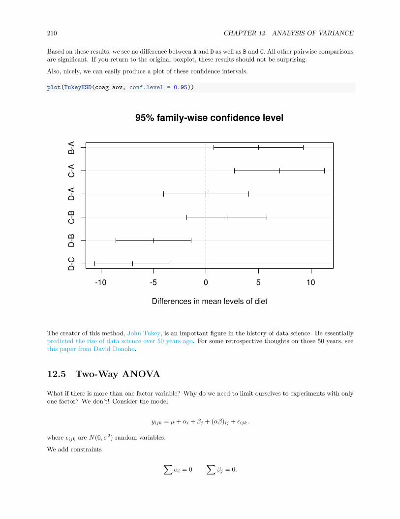
210 CHAPTER 12. ANALYSIS OF VARIANCE
Based on these results, we see no difference between A and D as well as B and C. All other pairwise comparisonsare significant. If you return to the original boxplot, these results should not be surprising.
Also, nicely, we can easily produce a plot of these confidence intervals.
plot(TukeyHSD(coag_aov, conf.level = 0.95))
-10 -5 0 5 10
D-C
D-B
C-B
D-A
C-A
B-A
95% family-wise confidence level
Differences in mean levels of diet
The creator of this method, John Tukey, is an important figure in the history of data science. He essentiallypredicted the rise of data science over 50 years ago. For some retrospective thoughts on those 50 years, seethis paper from David Donoho.
12.5 Two-Way ANOVA
What if there is more than one factor variable? Why do we need to limit ourselves to experiments with onlyone factor? We don’t! Consider the model
yijk = µ + αi + βj + (αβ)ij + ϵijk.
where ϵijk are N(0, σ2) random variables.
We add constraints
∑αi = 0
∑βj = 0.

12.5. TWO-WAY ANOVA 211
and
(αβ)1j + (αβ)2j + (αβ)3j = 0(αβ)i1 + (αβ)i2 + (αβ)i3 + (αβ)i4 = 0
for any i or j.
Here,
• i = 1, 2, . . . I where I is the number of levels of factor A.• j = 1, 2, . . . J where J is the number of levels of factor B.• k = 1, 2, . . . K where K is the number of replicates per group.
Here, we can think of a group as a combination of a level from each of the factors. So for example, one groupwill receive level 2 of factor A and level 3 of factor B. The number of replicates is the number of subjects ineach group. Here y135 would be the measurement for the fifth member (replicate) of the group for level 1 offactor A and level 3 of factor B.
We call this setup an I × J factorial design with K replicates. (Our current notation only allows forequal replicates in each group. It isn’t difficult to allow for different replicates for different groups, but we’llproceed using equal replicates per group, which if possible, is desirable.)
• αi measures the effect of level i of factor A. We call these the main effects of factor A.• βj measures the effect of level j of factor B. We call these the main effects of factor B.• (αβ)ij is a single parameter. We use αβ to note that this parameter measures the interaction between
the two main effects.
Under this setup, there are a number of models that we can compare. Consider a 2 × 2 factorial design. Thefollowing tables show the means for each of the possible groups under each model.
Interaction Model: yijk = µ + αi + βj + (αβ)ij + ϵijk
Factor B, Level 1 Factor B, Level 2Factor A, Level 1 µ + α1 + β1 + (αβ)11 µ + α1 + β2 + (αβ)12Factor A, Level 2 µ + α2 + β1 + (αβ)21 µ + α2 + β2 + (αβ)22
Additive Model: yijk = µ + αi + βj + ϵijk
Factor B, Level 1 Factor B, Level 2Factor A, Level 1 µ + α1 + β1 µ + α1 + β2Factor A, Level 2 µ + α2 + β1 µ + α2 + β2
Factor B Only Model (One-Way): yijk = µ + βj + ϵijk
Factor B, Level 1 Factor B, Level 2Factor A, Level 1 µ + β1 µ + β2Factor A, Level 2 µ + β1 µ + β2
Factor A Only Model (One-Way): yijk = µ + αi + ϵijk
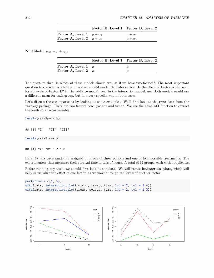
212 CHAPTER 12. ANALYSIS OF VARIANCE
Factor B, Level 1 Factor B, Level 2Factor A, Level 1 µ + α1 µ + α1Factor A, Level 2 µ + α2 µ + α2
Null Model: yijk = µ + ϵijk
Factor B, Level 1 Factor B, Level 2Factor A, Level 1 µ µFactor A, Level 2 µ µ
The question then, is which of these models should we use if we have two factors? The most importantquestion to consider is whether or not we should model the interaction. Is the effect of Factor A the samefor all levels of Factor B? In the additive model, yes. In the interaction model, no. Both models would usea different mean for each group, but in a very specific way in both cases.
Let’s discuss these comparisons by looking at some examples. We’ll first look at the rats data from thefaraway package. There are two factors here: poison and treat. We use the levels() function to extractthe levels of a factor variable.
levels(rats$poison)
## [1] "I" "II" "III"
levels(rats$treat)
## [1] "A" "B" "C" "D"
Here, 48 rats were randomly assigned both one of three poisons and one of four possible treatments. Theexperimenters then measures their survival time in tens of hours. A total of 12 groups, each with 4 replicates.
Before running any tests, we should first look at the data. We will create interaction plots, which willhelp us visualize the effect of one factor, as we move through the levels of another factor.
par(mfrow = c(1, 2))with(rats, interaction.plot(poison, treat, time, lwd = 2, col = 1:4))with(rats, interaction.plot(treat, poison, time, lwd = 2, col = 1:3))
0.2
0.3
0.4
0.5
0.6
0.7
0.8
0.9
poison
mea
n of
tim
e
I II III
treat
BDCA
0.2
0.3
0.4
0.5
0.6
0.7
0.8
0.9
treat
mea
n of
tim
e
A B C D
poison
IIIIII
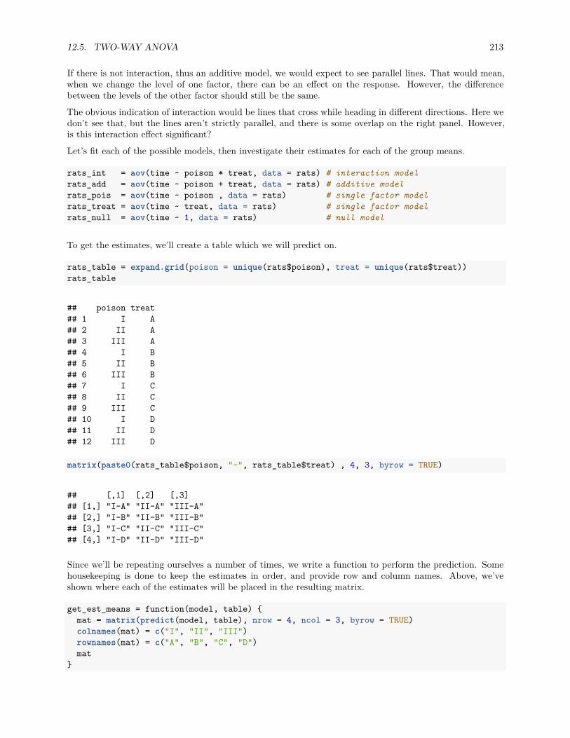
12.5. TWO-WAY ANOVA 213
If there is not interaction, thus an additive model, we would expect to see parallel lines. That would mean,when we change the level of one factor, there can be an effect on the response. However, the differencebetween the levels of the other factor should still be the same.
The obvious indication of interaction would be lines that cross while heading in different directions. Here wedon’t see that, but the lines aren’t strictly parallel, and there is some overlap on the right panel. However,is this interaction effect significant?
Let’s fit each of the possible models, then investigate their estimates for each of the group means.
rats_int = aov(time ~ poison * treat, data = rats) # interaction modelrats_add = aov(time ~ poison + treat, data = rats) # additive modelrats_pois = aov(time ~ poison , data = rats) # single factor modelrats_treat = aov(time ~ treat, data = rats) # single factor modelrats_null = aov(time ~ 1, data = rats) # null model
To get the estimates, we’ll create a table which we will predict on.
rats_table = expand.grid(poison = unique(rats$poison), treat = unique(rats$treat))rats_table
## poison treat## 1 I A## 2 II A## 3 III A## 4 I B## 5 II B## 6 III B## 7 I C## 8 II C## 9 III C## 10 I D## 11 II D## 12 III D
matrix(paste0(rats_table$poison, "-", rats_table$treat) , 4, 3, byrow = TRUE)
## [,1] [,2] [,3]## [1,] "I-A" "II-A" "III-A"## [2,] "I-B" "II-B" "III-B"## [3,] "I-C" "II-C" "III-C"## [4,] "I-D" "II-D" "III-D"
Since we’ll be repeating ourselves a number of times, we write a function to perform the prediction. Somehousekeeping is done to keep the estimates in order, and provide row and column names. Above, we’veshown where each of the estimates will be placed in the resulting matrix.
get_est_means = function(model, table) {mat = matrix(predict(model, table), nrow = 4, ncol = 3, byrow = TRUE)colnames(mat) = c("I", "II", "III")rownames(mat) = c("A", "B", "C", "D")mat
}

214 CHAPTER 12. ANALYSIS OF VARIANCE
First, we obtain the estimates from the interaction model. Note that each cell has a different value.
knitr::kable(get_est_means(model = rats_int, table = rats_table))
I II IIIA 0.4125 0.3200 0.210B 0.8800 0.8150 0.335C 0.5675 0.3750 0.235D 0.6100 0.6675 0.325
Next, we obtain the estimates from the additive model. Again, each cell has a different value. We also seethat these estimates are somewhat close to those from the interaction model.
knitr::kable(get_est_means(model = rats_add, table = rats_table))
I II IIIA 0.4522917 0.3791667 0.1110417B 0.8147917 0.7416667 0.4735417C 0.5306250 0.4575000 0.1893750D 0.6722917 0.5991667 0.3310417
To understand the difference, let’s consider the effect of the treatments.
additive_means = get_est_means(model = rats_add, table = rats_table)additive_means["A",] - additive_means["B",]
## I II III## -0.3625 -0.3625 -0.3625
interaction_means = get_est_means(model = rats_int, table = rats_table)interaction_means["A",] - interaction_means["B",]
## I II III## -0.4675 -0.4950 -0.1250
This is the key difference between the interaction and additive models. The difference between the effect oftreatments A and B is the same for each poison in the additive model. They are different in the interactionmodel.
The remaining three models are much simpler, having either only row or only column effects. Or no effectsin the case of the null model.
knitr::kable(get_est_means(model = rats_pois, table = rats_table))
I II IIIA 0.6175 0.544375 0.27625B 0.6175 0.544375 0.27625C 0.6175 0.544375 0.27625D 0.6175 0.544375 0.27625
knitr::kable(get_est_means(model = rats_treat, table = rats_table))
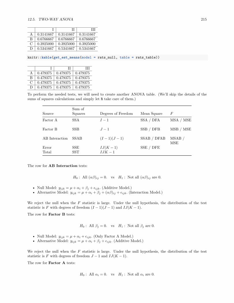
12.5. TWO-WAY ANOVA 215
I II IIIA 0.3141667 0.3141667 0.3141667B 0.6766667 0.6766667 0.6766667C 0.3925000 0.3925000 0.3925000D 0.5341667 0.5341667 0.5341667
knitr::kable(get_est_means(model = rats_null, table = rats_table))
I II IIIA 0.479375 0.479375 0.479375B 0.479375 0.479375 0.479375C 0.479375 0.479375 0.479375D 0.479375 0.479375 0.479375
To perform the needed tests, we will need to create another ANOVA table. (We’ll skip the details of thesums of squares calculations and simply let R take care of them.)
SourceSum ofSquares Degrees of Freedom Mean Square F
Factor A SSA I − 1 SSA / DFA MSA / MSE
Factor B SSB J − 1 SSB / DFB MSB / MSE
AB Interaction SSAB (I − 1)(J − 1) SSAB / DFAB MSAB /MSE
Error SSE IJ(K − 1) SSE / DFETotal SST IJK − 1
The row for AB Interaction tests:
H0 : All (αβ)ij = 0. vs H1 : Not all (αβ)ij are 0.
• Null Model: yijk = µ + αi + βj + ϵijk. (Additive Model.)• Alternative Model: yijk = µ + αi + βj + (αβ)ij + ϵijk. (Interaction Model.)
We reject the null when the F statistic is large. Under the null hypothesis, the distribution of the teststatistic is F with degrees of freedom (I − 1)(J − 1) and IJ(K − 1).
The row for Factor B tests:
H0 : All βj = 0. vs H1 : Not all βj are 0.
• Null Model: yijk = µ + αi + ϵijk. (Only Factor A Model.)• Alternative Model: yijk = µ + αi + βj + ϵijk. (Additive Model.)
We reject the null when the F statistic is large. Under the null hypothesis, the distribution of the teststatistic is F with degrees of freedom J − 1 and IJ(K − 1).
The row for Factor A tests:
H0 : All αi = 0. vs H1 : Not all αi are 0.
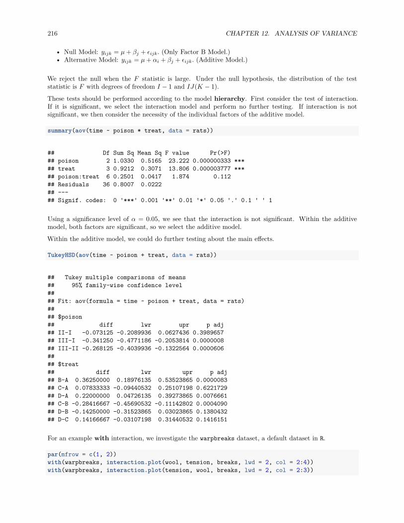
216 CHAPTER 12. ANALYSIS OF VARIANCE
• Null Model: yijk = µ + βj + ϵijk. (Only Factor B Model.)• Alternative Model: yijk = µ + αi + βj + ϵijk. (Additive Model.)
We reject the null when the F statistic is large. Under the null hypothesis, the distribution of the teststatistic is F with degrees of freedom I − 1 and IJ(K − 1).
These tests should be performed according to the model hierarchy. First consider the test of interaction.If it is significant, we select the interaction model and perform no further testing. If interaction is notsignificant, we then consider the necessity of the individual factors of the additive model.
summary(aov(time ~ poison * treat, data = rats))
## Df Sum Sq Mean Sq F value Pr(>F)## poison 2 1.0330 0.5165 23.222 0.000000333 ***## treat 3 0.9212 0.3071 13.806 0.000003777 ***## poison:treat 6 0.2501 0.0417 1.874 0.112## Residuals 36 0.8007 0.0222## ---## Signif. codes: 0 '***' 0.001 '**' 0.01 '*' 0.05 '.' 0.1 ' ' 1
Using a significance level of α = 0.05, we see that the interaction is not significant. Within the additivemodel, both factors are significant, so we select the additive model.
Within the additive model, we could do further testing about the main effects.
TukeyHSD(aov(time ~ poison + treat, data = rats))
## Tukey multiple comparisons of means## 95% family-wise confidence level#### Fit: aov(formula = time ~ poison + treat, data = rats)#### $poison## diff lwr upr p adj## II-I -0.073125 -0.2089936 0.0627436 0.3989657## III-I -0.341250 -0.4771186 -0.2053814 0.0000008## III-II -0.268125 -0.4039936 -0.1322564 0.0000606#### $treat## diff lwr upr p adj## B-A 0.36250000 0.18976135 0.53523865 0.0000083## C-A 0.07833333 -0.09440532 0.25107198 0.6221729## D-A 0.22000000 0.04726135 0.39273865 0.0076661## C-B -0.28416667 -0.45690532 -0.11142802 0.0004090## D-B -0.14250000 -0.31523865 0.03023865 0.1380432## D-C 0.14166667 -0.03107198 0.31440532 0.1416151
For an example with interaction, we investigate the warpbreaks dataset, a default dataset in R.
par(mfrow = c(1, 2))with(warpbreaks, interaction.plot(wool, tension, breaks, lwd = 2, col = 2:4))with(warpbreaks, interaction.plot(tension, wool, breaks, lwd = 2, col = 2:3))
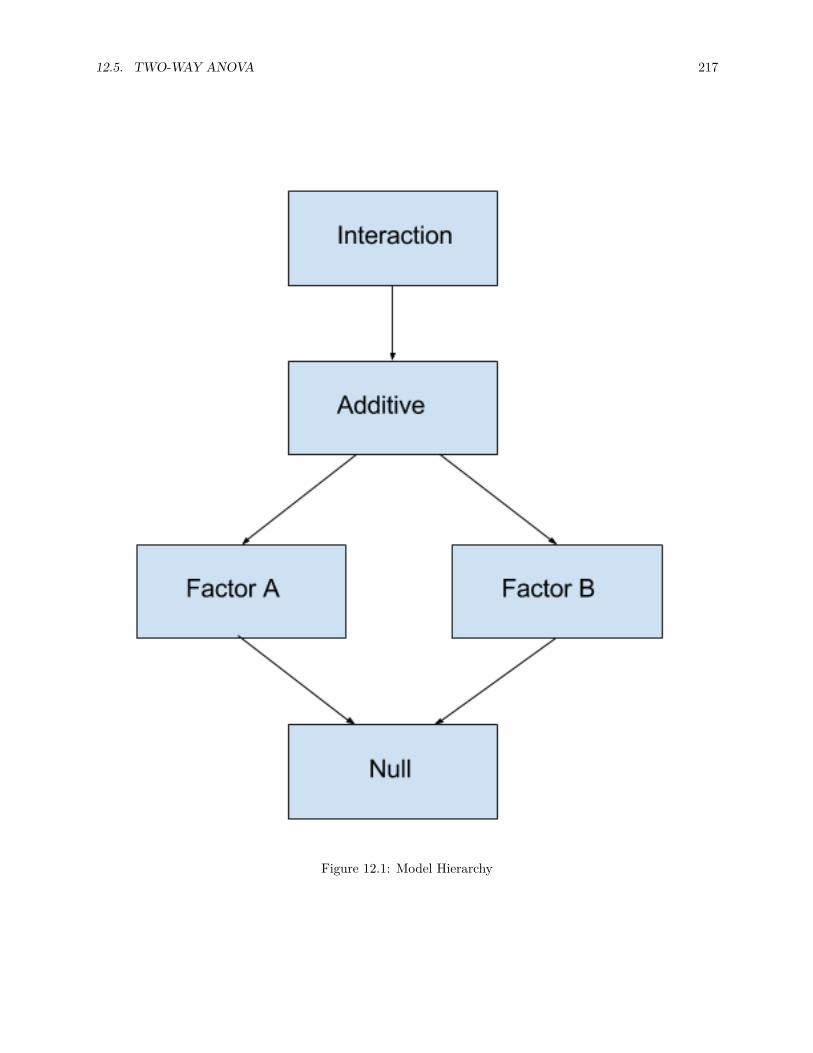
12.5. TWO-WAY ANOVA 217
Figure 12.1: Model Hierarchy
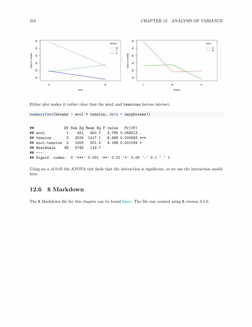
218 CHAPTER 12. ANALYSIS OF VARIANCE
2025
3035
4045
wool
mea
n of
bre
aks
A B
tension
MLH
2025
3035
4045
tension
mea
n of
bre
aks
L M H
wool
AB
Either plot makes it rather clear that the wool and tensions factors interact.
summary(aov(breaks ~ wool * tension, data = warpbreaks))
## Df Sum Sq Mean Sq F value Pr(>F)## wool 1 451 450.7 3.765 0.058213 .## tension 2 2034 1017.1 8.498 0.000693 ***## wool:tension 2 1003 501.4 4.189 0.021044 *## Residuals 48 5745 119.7## ---## Signif. codes: 0 '***' 0.001 '**' 0.01 '*' 0.05 '.' 0.1 ' ' 1
Using an α of 0.05 the ANOVA test finds that the interaction is significant, so we use the interaction modelhere.
12.6 R Markdown
The R Markdown file for this chapter can be found here. The file was created using R version 3.5.0.

Chapter 13
Model Diagnostics
“Your assumptions are your windows on the world. Scrub them off every once in a while, or thelight won’t come in.”
— Isaac Asimov
After reading this chapter you will be able to:
• Understand the assumptions of a regression model.• Assess regression model assumptions using visualizations and tests.• Understand leverage, outliers, and influential points.• Be able to identify unusual observations in regression models.
13.1 Model Assumptions
Recall the multiple linear regression model that we have defined.
Yi = β0 + β1xi1 + β2xi2 + · · · + βp−1xi(p−1) + ϵi, i = 1, 2, . . . , n.
Using matrix notation, this model can be written much more succinctly as
Y = Xβ + ϵ.
Given data, we found the estimates for the β parameters using
β =(X⊤X
)−1X⊤y.
We than noted that these estimates had mean
E[β] = β,
and variance
Var[β] = σ2 (X⊤X)−1
.
219

220 CHAPTER 13. MODEL DIAGNOSTICS
In particular, an individual parameter, say βj had a normal distribution
βj ∼ N(βj , σ2Cjj
)where C was the matrix defined as
C =(X⊤X
)−1.
We then used this fact to define
βj − βj
se
√Cjj
∼ tn−p,
which we used to perform hypothesis testing.
So far we have looked at various metrics such as RMSE, RSE and R2 to determine how well our model fitour data. Each of these in some way considers the expression
n∑i=1
(yi − yi)2.
So, essentially each of these looks at how close the data points are to the model. However is that all we careabout?
• It could be that the errors are made in a systematic way, which means that our model is misspecified.We may need additional interaction terms, or polynomial terms which we will see later.
• It is also possible that at a particular set of predictor values, the errors are very small, but at a differentset of predictor values, the errors are large.
• Perhaps most of the errors are very small, but some are very large. This would suggest that the errorsdo not follow a normal distribution.
Are these issues that we care about? If all we would like to do is predict, possibly not, since we would onlycare about the size of our errors. However, if we would like to perform inference, for example to determineif a particular predictor is important, we care a great deal. All of the distributional results, such as a t-testfor a single predictor, are derived under the assumptions of our model.
Technically, the assumptions of the model are encoded directly in a model statement such as,
Yi = β0 + β1xi1 + β2xi2 + · · · + βp−1xi(p−1) + ϵi
where ϵi ∼ N(0, σ2).
Often, the assumptions of linear regression, are stated as,
• Linearity: the response can be written as a linear combination of the predictors. (With noise aboutthis true linear relationship.)
• Independence: the errors are independent.• Normality: the distribution of the errors should follow a normal distribution.• Equal Variance: the error variance is the same at any set of predictor values.

13.2. CHECKING ASSUMPTIONS 221
The linearity assumption is encoded as
β0 + β1xi1 + β2xi2 + · · · + βp−1xi(p−1),
while the remaining three, are all encoded in
ϵi ∼ N(0, σ2),
since the ϵi are iid normal random variables with constant variance.
If these assumptions are met, great! We can perform inference, and it is valid. If these assumptions are notmet, we can still “perform” a t-test using R, but the results are not valid. The distributions of the parameterestimates will not be what we expect. Hypothesis tests will then accept or reject incorrectly. Essentially,garbage in, garbage out.
13.2 Checking Assumptions
We’ll now look at a number of tools for checking the assumptions of a linear model. To test these tools, we’lluse data simulated from three models:
Model 1: Y = 3 + 5x + ϵ, ϵ ∼ N(0, 1)
Model 2: Y = 3 + 5x + ϵ, ϵ ∼ N(0, x2)
Model 3: Y = 3 + 5x2 + ϵ, ϵ ∼ N(0, 25)
sim_1 = function(sample_size = 500) {x = runif(n = sample_size) * 5y = 3 + 5 * x + rnorm(n = sample_size, mean = 0, sd = 1)data.frame(x, y)
}
sim_2 = function(sample_size = 500) {x = runif(n = sample_size) * 5y = 3 + 5 * x + rnorm(n = sample_size, mean = 0, sd = x)data.frame(x, y)
}
sim_3 = function(sample_size = 500) {x = runif(n = sample_size) * 5y = 3 + 5 * x ^ 2 + rnorm(n = sample_size, mean = 0, sd = 5)data.frame(x, y)
}
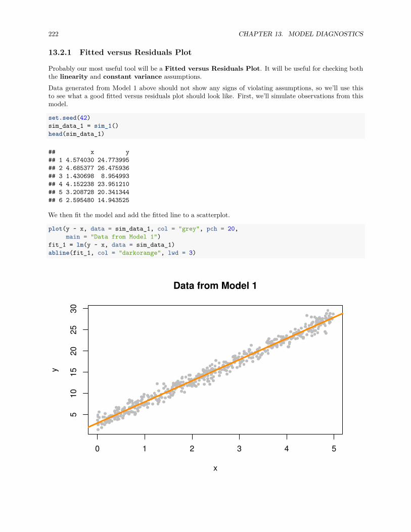
222 CHAPTER 13. MODEL DIAGNOSTICS
13.2.1 Fitted versus Residuals Plot
Probably our most useful tool will be a Fitted versus Residuals Plot. It will be useful for checking boththe linearity and constant variance assumptions.Data generated from Model 1 above should not show any signs of violating assumptions, so we’ll use thisto see what a good fitted versus residuals plot should look like. First, we’ll simulate observations from thismodel.
set.seed(42)sim_data_1 = sim_1()head(sim_data_1)
## x y## 1 4.574030 24.773995## 2 4.685377 26.475936## 3 1.430698 8.954993## 4 4.152238 23.951210## 5 3.208728 20.341344## 6 2.595480 14.943525
We then fit the model and add the fitted line to a scatterplot.
plot(y ~ x, data = sim_data_1, col = "grey", pch = 20,main = "Data from Model 1")
fit_1 = lm(y ~ x, data = sim_data_1)abline(fit_1, col = "darkorange", lwd = 3)
0 1 2 3 4 5
510
1520
2530
Data from Model 1
x
y
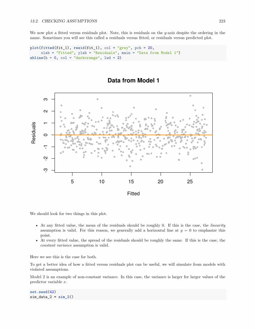
13.2. CHECKING ASSUMPTIONS 223
We now plot a fitted versus residuals plot. Note, this is residuals on the y-axis despite the ordering in thename. Sometimes you will see this called a residuals versus fitted, or residuals versus predicted plot.
plot(fitted(fit_1), resid(fit_1), col = "grey", pch = 20,xlab = "Fitted", ylab = "Residuals", main = "Data from Model 1")
abline(h = 0, col = "darkorange", lwd = 2)
5 10 15 20 25
-3-2
-10
12
3
Data from Model 1
Fitted
Res
idua
ls
We should look for two things in this plot.
• At any fitted value, the mean of the residuals should be roughly 0. If this is the case, the linearityassumption is valid. For this reason, we generally add a horizontal line at y = 0 to emphasize thispoint.
• At every fitted value, the spread of the residuals should be roughly the same. If this is the case, theconstant variance assumption is valid.
Here we see this is the case for both.
To get a better idea of how a fitted versus residuals plot can be useful, we will simulate from models withviolated assumptions.
Model 2 is an example of non-constant variance. In this case, the variance is larger for larger values of thepredictor variable x.
set.seed(42)sim_data_2 = sim_2()
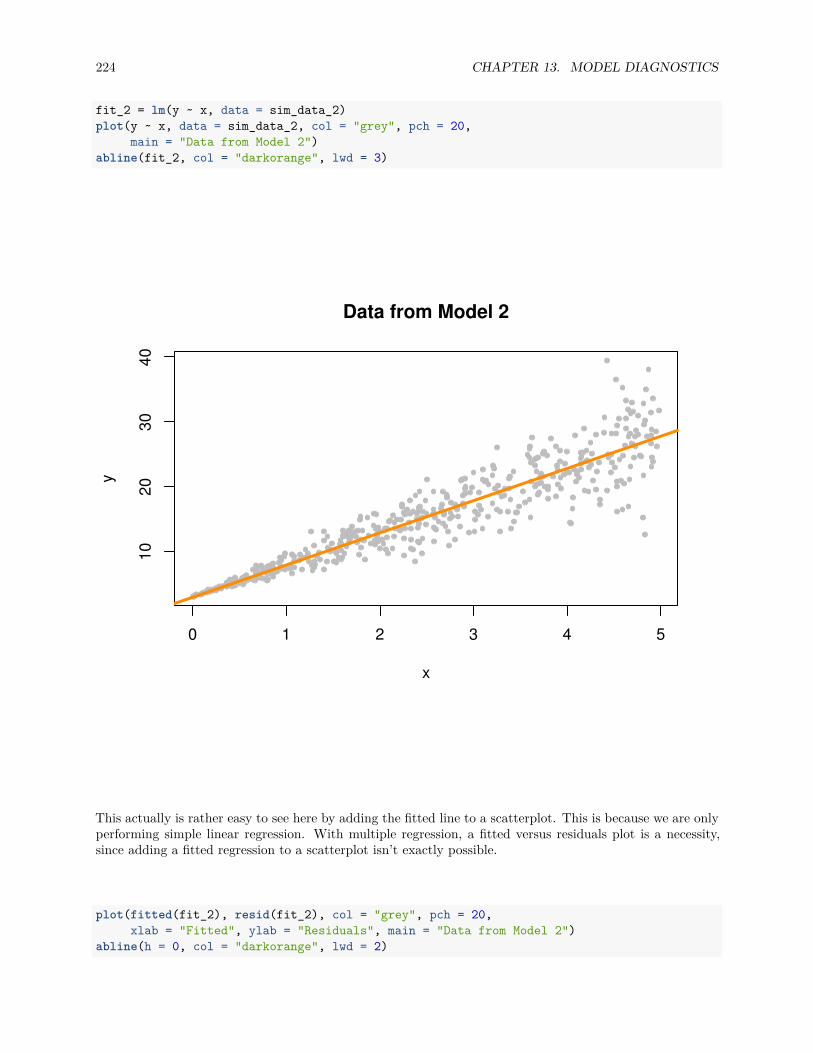
224 CHAPTER 13. MODEL DIAGNOSTICS
fit_2 = lm(y ~ x, data = sim_data_2)plot(y ~ x, data = sim_data_2, col = "grey", pch = 20,
main = "Data from Model 2")abline(fit_2, col = "darkorange", lwd = 3)
0 1 2 3 4 5
1020
3040
Data from Model 2
x
y
This actually is rather easy to see here by adding the fitted line to a scatterplot. This is because we are onlyperforming simple linear regression. With multiple regression, a fitted versus residuals plot is a necessity,since adding a fitted regression to a scatterplot isn’t exactly possible.
plot(fitted(fit_2), resid(fit_2), col = "grey", pch = 20,xlab = "Fitted", ylab = "Residuals", main = "Data from Model 2")
abline(h = 0, col = "darkorange", lwd = 2)
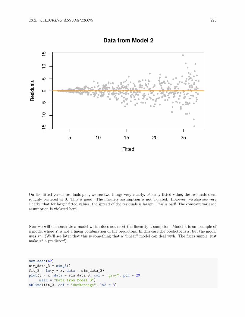
13.2. CHECKING ASSUMPTIONS 225
5 10 15 20 25
-15
-10
-50
510
15Data from Model 2
Fitted
Res
idua
ls
On the fitted versus residuals plot, we see two things very clearly. For any fitted value, the residuals seemroughly centered at 0. This is good! The linearity assumption is not violated. However, we also see veryclearly, that for larger fitted values, the spread of the residuals is larger. This is bad! The constant varianceassumption is violated here.
Now we will demonstrate a model which does not meet the linearity assumption. Model 3 is an example ofa model where Y is not a linear combination of the predictors. In this case the predictor is x, but the modeluses x2. (We’ll see later that this is something that a “linear” model can deal with. The fix is simple, justmake x2 a predictor!)
set.seed(42)sim_data_3 = sim_3()fit_3 = lm(y ~ x, data = sim_data_3)plot(y ~ x, data = sim_data_3, col = "grey", pch = 20,
main = "Data from Model 3")abline(fit_3, col = "darkorange", lwd = 3)
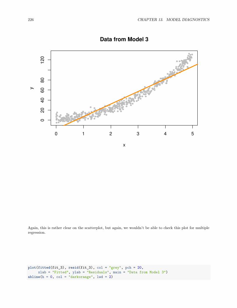
226 CHAPTER 13. MODEL DIAGNOSTICS
0 1 2 3 4 5
020
4060
8012
0Data from Model 3
x
y
Again, this is rather clear on the scatterplot, but again, we wouldn’t be able to check this plot for multipleregression.
plot(fitted(fit_3), resid(fit_3), col = "grey", pch = 20,xlab = "Fitted", ylab = "Residuals", main = "Data from Model 3")
abline(h = 0, col = "darkorange", lwd = 2)
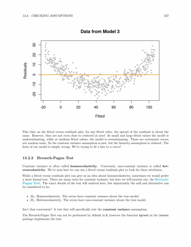
13.2. CHECKING ASSUMPTIONS 227
-20 0 20 40 60 80 100
-20
-10
010
2030
Data from Model 3
Fitted
Res
idua
ls
This time on the fitted versus residuals plot, for any fitted value, the spread of the residuals is about thesame. However, they are not even close to centered at zero! At small and large fitted values the model isunderestimating, while at medium fitted values, the model is overestimating. These are systematic errors,not random noise. So the constant variance assumption is met, but the linearity assumption is violated. Theform of our model is simply wrong. We’re trying to fit a line to a curve!
13.2.2 Breusch-Pagan Test
Constant variance is often called homoscedasticity. Conversely, non-constant variance is called het-eroscedasticity. We’ve seen how we can use a fitted versus residuals plot to look for these attributes.
While a fitted versus residuals plot can give us an idea about homoscedasticity, sometimes we would prefera more formal test. There are many tests for constant variance, but here we will present one, the Breusch-Pagan Test. The exact details of the test will omitted here, but importantly the null and alternative canbe considered to be,
• H0: Homoscedasticity. The errors have constant variance about the true model.• H1: Heteroscedasticity. The errors have non-constant variance about the true model.
Isn’t that convenient? A test that will specifically test the constant variance assumption.
The Breusch-Pagan Test can not be performed by default in R, however the function bptest in the lmtestpackage implements the test.
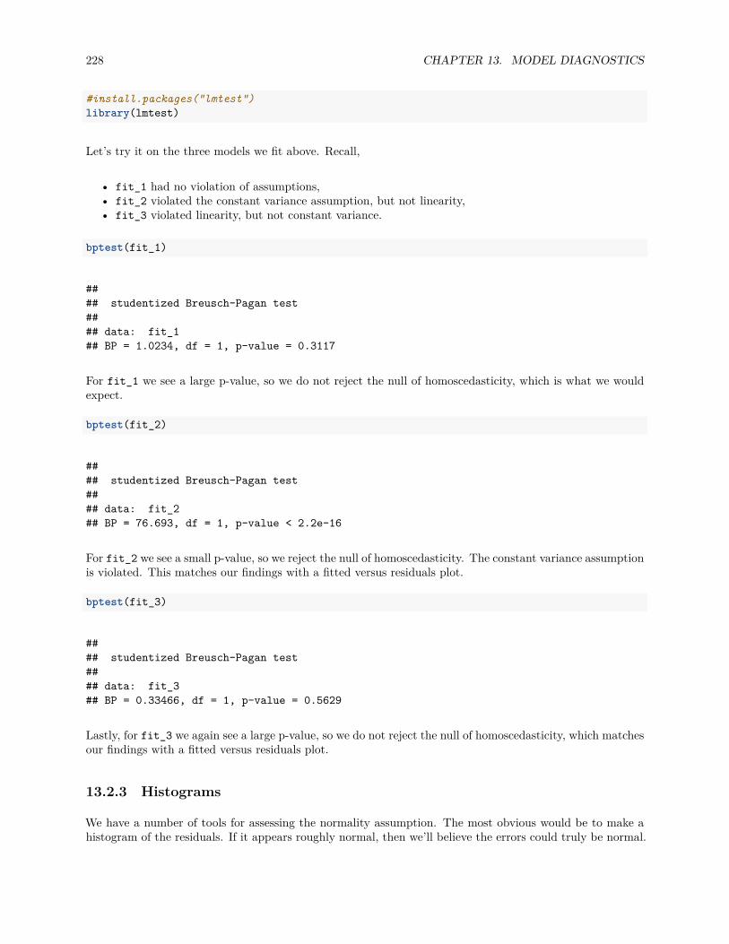
228 CHAPTER 13. MODEL DIAGNOSTICS
#install.packages("lmtest")library(lmtest)
Let’s try it on the three models we fit above. Recall,
• fit_1 had no violation of assumptions,• fit_2 violated the constant variance assumption, but not linearity,• fit_3 violated linearity, but not constant variance.
bptest(fit_1)
#### studentized Breusch-Pagan test#### data: fit_1## BP = 1.0234, df = 1, p-value = 0.3117
For fit_1 we see a large p-value, so we do not reject the null of homoscedasticity, which is what we wouldexpect.
bptest(fit_2)
#### studentized Breusch-Pagan test#### data: fit_2## BP = 76.693, df = 1, p-value < 2.2e-16
For fit_2 we see a small p-value, so we reject the null of homoscedasticity. The constant variance assumptionis violated. This matches our findings with a fitted versus residuals plot.
bptest(fit_3)
#### studentized Breusch-Pagan test#### data: fit_3## BP = 0.33466, df = 1, p-value = 0.5629
Lastly, for fit_3 we again see a large p-value, so we do not reject the null of homoscedasticity, which matchesour findings with a fitted versus residuals plot.
13.2.3 Histograms
We have a number of tools for assessing the normality assumption. The most obvious would be to make ahistogram of the residuals. If it appears roughly normal, then we’ll believe the errors could truly be normal.

13.2. CHECKING ASSUMPTIONS 229
par(mfrow = c(1, 3))hist(resid(fit_1),
xlab = "Residuals",main = "Histogram of Residuals, fit_1",col = "darkorange",border = "dodgerblue",breaks = 20)
hist(resid(fit_2),xlab = "Residuals",main = "Histogram of Residuals, fit_2",col = "darkorange",border = "dodgerblue",breaks = 20)
hist(resid(fit_3),xlab = "Residuals",main = "Histogram of Residuals, fit_3",col = "darkorange",border = "dodgerblue",breaks = 20)
Histogram of Residuals, fit_1
Residuals
Freq
uenc
y
-3 -2 -1 0 1 2 3
020
4060
8010
0
Histogram of Residuals, fit_2
Residuals
Freq
uenc
y
-15 -10 -5 0 5 10 15
050
100
150
Histogram of Residuals, fit_3
Residuals
Freq
uenc
y
-20 -10 0 10 20 30
010
2030
40
Above are histograms for each of the three regression we have been considering. Notice that the first, forfit_1 appears very normal. The third, for fit_3, appears to be very non-normal. However fit_2 is notas clear. It does have a rough bell shape, however, it also has a very sharp peak. For this reason we willusually use more powerful tools such as Q-Q plots and the Shapiro-Wilk test for assessing the normalityof errors.
13.2.4 Q-Q Plots
Another visual method for assessing the normality of errors, which is more powerful than a histogram, is anormal quantile-quantile plot, or Q-Q plot for short.
In R these are very easy to make. The qqnorm() function plots the points, and the qqline() function addsthe necessary line. We create a Q-Q plot for the residuals of fit_1 to check if the errors could truly benormally distributed.
qqnorm(resid(fit_1), main = "Normal Q-Q Plot, fit_1", col = "darkgrey")qqline(resid(fit_1), col = "dodgerblue", lwd = 2)

230 CHAPTER 13. MODEL DIAGNOSTICS
-3 -2 -1 0 1 2 3
-3-2
-10
12
3Normal Q-Q Plot, fit_1
Theoretical Quantiles
Sam
ple
Qua
ntile
s
In short, if the points of the plot do not closely follow a straight line, this would suggest that the data donot come from a normal distribution.
The calculations required to create the plot vary depending on the implementation, but essentially the y-axisis the sorted data (observed, or sample quantiles), and the x-axis is the values we would expect if the datadid come from a normal distribution (theoretical quantiles).
The Wikipedia page for Normal probability plots gives details on how this is implemented in R if you areinterested.
Also, to get a better idea of how Q-Q plots work, here is a quick function which creates a Q-Q plot:
qq_plot = function(e) {
n = length(e)normal_quantiles = qnorm(((1:n - 0.5) / n))# normal_quantiles = qnorm(((1:n) / (n + 1)))
# plot theoretical verus observed quantilesplot(normal_quantiles, sort(e),
xlab = c("Theoretical Quantiles"),ylab = c("Sample Quantiles"),col = "darkgrey")
title("Normal Q-Q Plot")
# calculate line through the first and third quartilesslope = (quantile(e, 0.75) - quantile(e, 0.25)) / (qnorm(0.75) - qnorm(0.25))
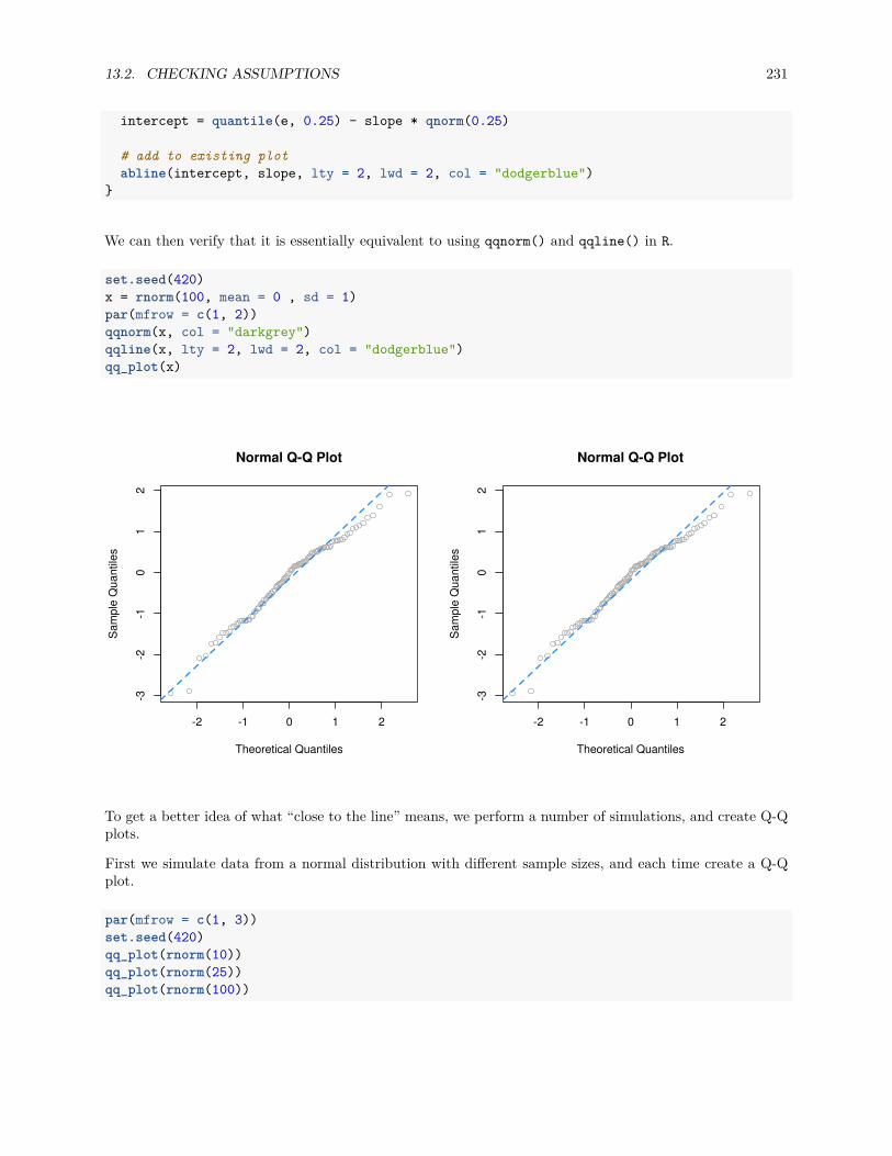
13.2. CHECKING ASSUMPTIONS 231
intercept = quantile(e, 0.25) - slope * qnorm(0.25)
# add to existing plotabline(intercept, slope, lty = 2, lwd = 2, col = "dodgerblue")
}
We can then verify that it is essentially equivalent to using qqnorm() and qqline() in R.
set.seed(420)x = rnorm(100, mean = 0 , sd = 1)par(mfrow = c(1, 2))qqnorm(x, col = "darkgrey")qqline(x, lty = 2, lwd = 2, col = "dodgerblue")qq_plot(x)
-2 -1 0 1 2
-3-2
-10
12
Normal Q-Q Plot
Theoretical Quantiles
Sam
ple
Qua
ntile
s
-2 -1 0 1 2
-3-2
-10
12
Theoretical Quantiles
Sam
ple
Qua
ntile
sNormal Q-Q Plot
To get a better idea of what “close to the line” means, we perform a number of simulations, and create Q-Qplots.
First we simulate data from a normal distribution with different sample sizes, and each time create a Q-Qplot.
par(mfrow = c(1, 3))set.seed(420)qq_plot(rnorm(10))qq_plot(rnorm(25))qq_plot(rnorm(100))
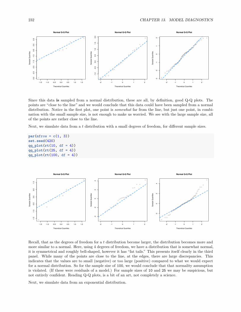
232 CHAPTER 13. MODEL DIAGNOSTICS
-1.5 -1.0 -0.5 0.0 0.5 1.0 1.5
-3.0
-2.5
-2.0
-1.5
-1.0
-0.5
0.0
0.5
Theoretical Quantiles
Sam
ple
Qua
ntile
s
Normal Q-Q Plot
-2 -1 0 1 2
-1.0
-0.5
0.0
0.5
1.0
1.5
2.0
Theoretical Quantiles
Sam
ple
Qua
ntile
s
Normal Q-Q Plot
-2 -1 0 1 2
-3-2
-10
12
Theoretical Quantiles
Sam
ple
Qua
ntile
s
Normal Q-Q Plot
Since this data is sampled from a normal distribution, these are all, by definition, good Q-Q plots. Thepoints are “close to the line” and we would conclude that this data could have been sampled from a normaldistribution. Notice in the first plot, one point is somewhat far from the line, but just one point, in combi-nation with the small sample size, is not enough to make us worried. We see with the large sample size, allof the points are rather close to the line.
Next, we simulate data from a t distribution with a small degrees of freedom, for different sample sizes.
par(mfrow = c(1, 3))set.seed(420)qq_plot(rt(10, df = 4))qq_plot(rt(25, df = 4))qq_plot(rt(100, df = 4))
-1.5 -1.0 -0.5 0.0 0.5 1.0 1.5
-1.5
-1.0
-0.5
0.0
0.5
1.0
Theoretical Quantiles
Sam
ple
Qua
ntile
s
Normal Q-Q Plot
-2 -1 0 1 2
-4-2
02
4
Theoretical Quantiles
Sam
ple
Qua
ntile
s
Normal Q-Q Plot
-2 -1 0 1 2
-20
24
Theoretical Quantiles
Sam
ple
Qua
ntile
s
Normal Q-Q Plot
Recall, that as the degrees of freedom for a t distribution become larger, the distribution becomes more andmore similar to a normal. Here, using 4 degrees of freedom, we have a distribution that is somewhat normal,it is symmetrical and roughly bell-shaped, however it has “fat tails.” This presents itself clearly in the thirdpanel. While many of the points are close to the line, at the edges, there are large discrepancies. Thisindicates that the values are to small (negative) or too large (positive) compared to what we would expectfor a normal distribution. So for the sample size of 100, we would conclude that that normality assumptionis violated. (If these were residuals of a model.) For sample sizes of 10 and 25 we may be suspicious, butnot entirely confident. Reading Q-Q plots, is a bit of an art, not completely a science.
Next, we simulate data from an exponential distribution.
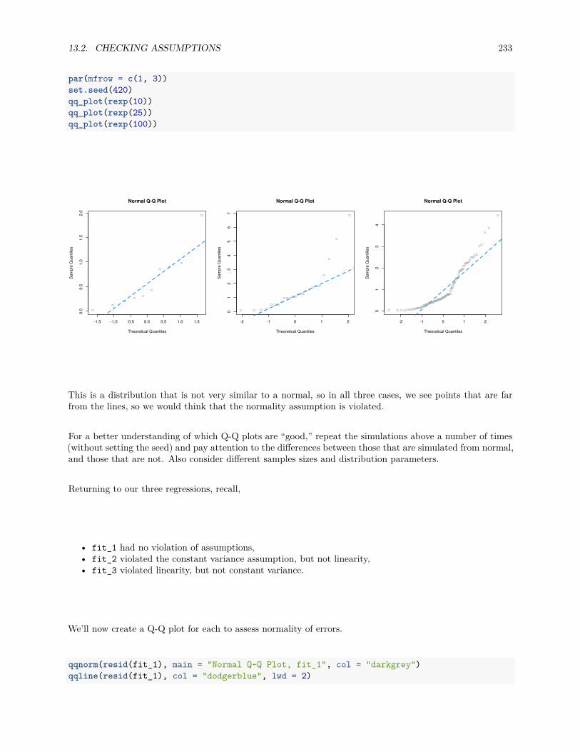
13.2. CHECKING ASSUMPTIONS 233
par(mfrow = c(1, 3))set.seed(420)qq_plot(rexp(10))qq_plot(rexp(25))qq_plot(rexp(100))
-1.5 -1.0 -0.5 0.0 0.5 1.0 1.5
0.0
0.5
1.0
1.5
2.0
Theoretical Quantiles
Sam
ple
Qua
ntile
s
Normal Q-Q Plot
-2 -1 0 1 2
01
23
45
67
Theoretical Quantiles
Sam
ple
Qua
ntile
s
Normal Q-Q Plot
-2 -1 0 1 2
01
23
4
Theoretical Quantiles
Sam
ple
Qua
ntile
s
Normal Q-Q Plot
This is a distribution that is not very similar to a normal, so in all three cases, we see points that are farfrom the lines, so we would think that the normality assumption is violated.
For a better understanding of which Q-Q plots are “good,” repeat the simulations above a number of times(without setting the seed) and pay attention to the differences between those that are simulated from normal,and those that are not. Also consider different samples sizes and distribution parameters.
Returning to our three regressions, recall,
• fit_1 had no violation of assumptions,• fit_2 violated the constant variance assumption, but not linearity,• fit_3 violated linearity, but not constant variance.
We’ll now create a Q-Q plot for each to assess normality of errors.
qqnorm(resid(fit_1), main = "Normal Q-Q Plot, fit_1", col = "darkgrey")qqline(resid(fit_1), col = "dodgerblue", lwd = 2)

234 CHAPTER 13. MODEL DIAGNOSTICS
-3 -2 -1 0 1 2 3
-3-2
-10
12
3Normal Q-Q Plot, fit_1
Theoretical Quantiles
Sam
ple
Qua
ntile
s
For fit_1, we have a near perfect Q-Q plot. We would believe the errors follow a normal distribution.
qqnorm(resid(fit_2), main = "Normal Q-Q Plot, fit_2", col = "darkgrey")qqline(resid(fit_2), col = "dodgerblue", lwd = 2)
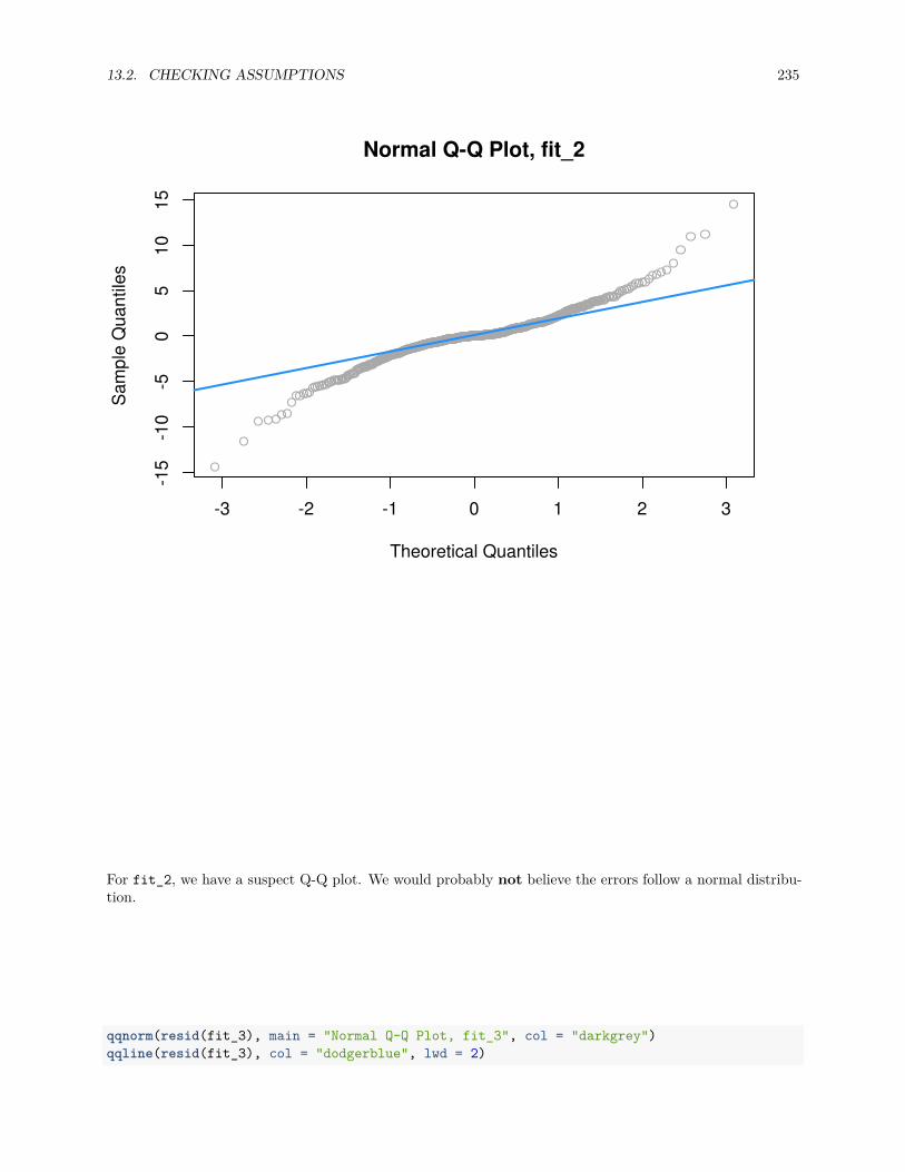
13.2. CHECKING ASSUMPTIONS 235
-3 -2 -1 0 1 2 3
-15
-10
-50
510
15Normal Q-Q Plot, fit_2
Theoretical Quantiles
Sam
ple
Qua
ntile
s
For fit_2, we have a suspect Q-Q plot. We would probably not believe the errors follow a normal distribu-tion.
qqnorm(resid(fit_3), main = "Normal Q-Q Plot, fit_3", col = "darkgrey")qqline(resid(fit_3), col = "dodgerblue", lwd = 2)

236 CHAPTER 13. MODEL DIAGNOSTICS
-3 -2 -1 0 1 2 3
-20
-10
010
2030
Normal Q-Q Plot, fit_3
Theoretical Quantiles
Sam
ple
Qua
ntile
s
Lastly, for fit_3, we again have a suspect Q-Q plot. We would probably not believe the errors follow anormal distribution.
13.2.5 Shapiro-Wilk Test
Histograms and Q-Q Plots give a nice visual representation of the residuals distribution, however if weare interested in formal testing, there are a number of options available. A commonly used test is theShapiro–Wilk test, which is implemented in R.
set.seed(42)shapiro.test(rnorm(25))
#### Shapiro-Wilk normality test#### data: rnorm(25)## W = 0.9499, p-value = 0.2495
shapiro.test(rexp(25))
#### Shapiro-Wilk normality test#### data: rexp(25)## W = 0.71164, p-value = 0.0000105

13.3. UNUSUAL OBSERVATIONS 237
This gives us the value of the test statistic and its p-value. The null hypothesis assumes the data were sampledfrom a normal distribution, thus a small p-value indicates we believe there is only a small probability thedata could have been sampled from a normal distribution.
For details, see: Wikipedia: Shapiro–Wilk test.
In the above examples, we see we fail to reject for the data sampled from normal, and reject on the non-normaldata, for any reasonable α.
Returning again to fit_1, fit_2 and fit_3, we see the result of running shapiro.test() on the residualsof each, returns a result for each that matches for decisions based on the Q-Q plots.
shapiro.test(resid(fit_1))
#### Shapiro-Wilk normality test#### data: resid(fit_1)## W = 0.99858, p-value = 0.9622
shapiro.test(resid(fit_2))
#### Shapiro-Wilk normality test#### data: resid(fit_2)## W = 0.93697, p-value = 1.056e-13
shapiro.test(resid(fit_3))
#### Shapiro-Wilk normality test#### data: resid(fit_3)## W = 0.97643, p-value = 0.0000003231
13.3 Unusual Observations
In addition to checking the assumptions of regression, we also look for any “unusual observations” in thedata. Often a small number of data points can have an extremely large influence on a regression, sometimesso much so that the regression assumptions are violated as a result of these points.
The following three plots are inspired by an example from Linear Models with R.
par(mfrow = c(1, 3))set.seed(42)ex_data = data.frame(x = 1:10,
y = 10:1 + rnorm(n = 10))ex_model = lm(y ~ x, data = ex_data)
# low leverage, large residual, small influencepoint_1 = c(5.4, 11)
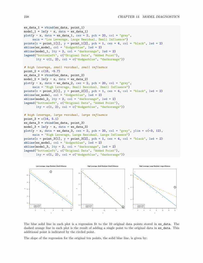
238 CHAPTER 13. MODEL DIAGNOSTICS
ex_data_1 = rbind(ex_data, point_1)model_1 = lm(y ~ x, data = ex_data_1)plot(y ~ x, data = ex_data_1, cex = 2, pch = 20, col = "grey",
main = "Low Leverage, Large Residual, Small Influence")points(x = point_1[1], y = point_1[2], pch = 1, cex = 4, col = "black", lwd = 2)abline(ex_model, col = "dodgerblue", lwd = 2)abline(model_1, lty = 2, col = "darkorange", lwd = 2)legend("bottomleft", c("Original Data", "Added Point"),
lty = c(1, 2), col = c("dodgerblue", "darkorange"))
# high leverage, small residual, small influencepoint_2 = c(18, -5.7)ex_data_2 = rbind(ex_data, point_2)model_2 = lm(y ~ x, data = ex_data_2)plot(y ~ x, data = ex_data_2, cex = 2, pch = 20, col = "grey",
main = "High Leverage, Small Residual, Small Influence")points(x = point_2[1], y = point_2[2], pch = 1, cex = 4, col = "black", lwd = 2)abline(ex_model, col = "dodgerblue", lwd = 2)abline(model_2, lty = 2, col = "darkorange", lwd = 2)legend("bottomleft", c("Original Data", "Added Point"),
lty = c(1, 2), col = c("dodgerblue", "darkorange"))
# high leverage, large residual, large influencepoint_3 = c(14, 5.1)ex_data_3 = rbind(ex_data, point_3)model_3 = lm(y ~ x, data = ex_data_3)plot(y ~ x, data = ex_data_3, cex = 2, pch = 20, col = "grey", ylim = c(-3, 12),
main = "High Leverage, Large Residual, Large Influence")points(x = point_3[1], y = point_3[2], pch = 1, cex = 4, col = "black", lwd = 2)abline(ex_model, col = "dodgerblue", lwd = 2)abline(model_3, lty = 2, col = "darkorange", lwd = 2)legend("bottomleft", c("Original Data", "Added Point"),
lty = c(1, 2), col = c("dodgerblue", "darkorange"))
2 4 6 8 10
24
68
10
Low Leverage, Large Residual, Small Influence
x
y
Original DataAdded Point
5 10 15
-50
510
High Leverage, Small Residual, Small Influence
x
y
Original DataAdded Point
2 4 6 8 10 12 14
05
10
High Leverage, Large Residual, Large Influence
x
y
Original DataAdded Point
The blue solid line in each plot is a regression fit to the 10 original data points stored in ex_data. Thedashed orange line in each plot is the result of adding a single point to the original data in ex_data. Thisadditional point is indicated by the circled point.
The slope of the regression for the original ten points, the solid blue line, is given by:

13.3. UNUSUAL OBSERVATIONS 239
coef(ex_model)[2]
## x## -0.9696033
The added point in the first plot has a small effect on the slope, which becomes:
coef(model_1)[2]
## x## -0.9749534
We will say that this point has low leverage, is an outlier due to its large residual, but has small influence.
The added point in the second plot also has a small effect on the slope, which is:
coef(model_2)[2]
## x## -0.9507397
We will say that this point has high leverage, is not an outlier due to its small residual, and has a very smallinfluence.
Lastly, the added point in the third plot has a large effect on the slope, which is now:
coef(model_3)[2]
## x## -0.5892241
This added point is influential. It both has high leverage, and is an outlier due to its large residual.
We’ve now mentioned three new concepts: leverage, outliers, and influential points, each of which we willdiscuss in detail.
13.3.1 Leverage
A data point with high leverage, is a data point that could have a large influence when fitting the model.
Recall that,
β =(X⊤X
)−1X⊤y.
Thus,
y = Xβ = X(X⊤X
)−1X⊤y
Now we define,

240 CHAPTER 13. MODEL DIAGNOSTICS
H = X(X⊤X
)−1X⊤
which we will refer to as the hat matrix. The hat matrix is used to project onto the subspace spanned bythe columns of X. It is also simply known as a projection matrix.
The hat matrix, is a matrix that takes the original y values, and adds a hat!
y = Hy
The diagonal elements of this matrix are called the leverages
Hii = hi,
where hi is the leverage for the ith observation.
Large values of hi indicate extreme values in X, which may influence regression. Note that leverages onlydepend on X.
Here, p the number of βs is also the trace (and rank) of the hat matrix.
n∑i=1
hi = p
What is a value of hi that would be considered large? There is no exact answer to this question. A commonheuristic would be to compare each leverage to two times the average leverage. A leverage larger than thisis considered an observation to be aware of. That is, if
hi > 2h
we say that observation i has large leverage. Here,
h =∑n
i=1 hi
n= p
n.
For simple linear regression, the leverage for each point is given by
hi = 1n
+ (xi − x)2
Sxx.
This expression should be familiar. (Think back to inference for SLR.) It suggests that the large leveragesoccur when x values are far from their mean. Recall that the regression goes through the point (x, y).
There are multiple ways to find leverages in R.
lev_ex = data.frame(x1 = c(0, 11, 11, 7, 4, 10, 5, 8),x2 = c(1, 5, 4, 3, 1, 4, 4, 2),y = c(11, 15, 13, 14, 0, 19, 16, 8))
plot(x2 ~ x1, data = lev_ex, cex = 2)points(7, 3, pch = 20, col = "red", cex = 2)
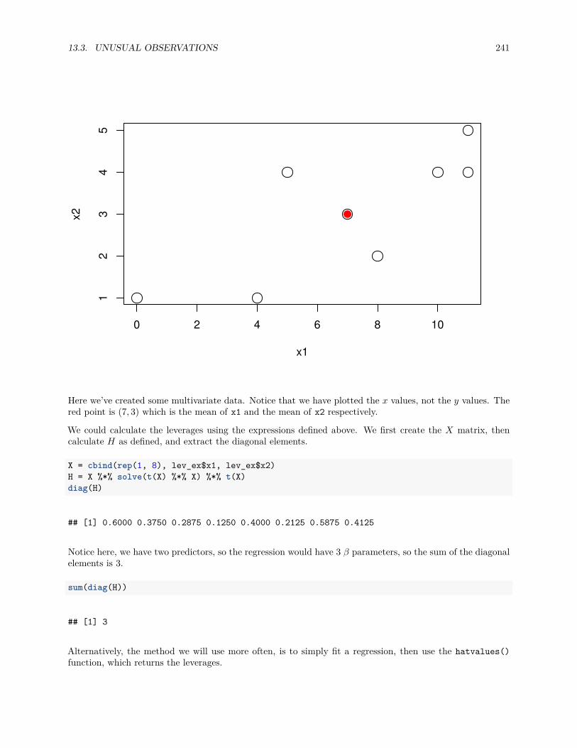
13.3. UNUSUAL OBSERVATIONS 241
0 2 4 6 8 10
12
34
5
x1
x2
Here we’ve created some multivariate data. Notice that we have plotted the x values, not the y values. Thered point is (7, 3) which is the mean of x1 and the mean of x2 respectively.
We could calculate the leverages using the expressions defined above. We first create the X matrix, thencalculate H as defined, and extract the diagonal elements.
X = cbind(rep(1, 8), lev_ex$x1, lev_ex$x2)H = X %*% solve(t(X) %*% X) %*% t(X)diag(H)
## [1] 0.6000 0.3750 0.2875 0.1250 0.4000 0.2125 0.5875 0.4125
Notice here, we have two predictors, so the regression would have 3 β parameters, so the sum of the diagonalelements is 3.
sum(diag(H))
## [1] 3
Alternatively, the method we will use more often, is to simply fit a regression, then use the hatvalues()function, which returns the leverages.

242 CHAPTER 13. MODEL DIAGNOSTICS
lev_fit = lm(y ~ ., data = lev_ex)hatvalues(lev_fit)
## 1 2 3 4 5 6 7 8## 0.6000 0.3750 0.2875 0.1250 0.4000 0.2125 0.5875 0.4125
Again, note that here we have “used” the y values to fit the regression, but R still ignores them whencalculating the leverages, as leverages only depend on the x values.
coef(lev_fit)
## (Intercept) x1 x2## 3.7 -0.7 4.4
Let’s see what happens to these coefficients when we modify the y value of the point with the highest leverage.
which.max(hatvalues(lev_fit))
## 1## 1
lev_ex[which.max(hatvalues(lev_fit)),]
## x1 x2 y## 1 0 1 11
We see that the original y value is 11. We’ll create a copy of the data, and modify this point to have a yvalue of 20.
lev_ex_1 = lev_exlev_ex_1$y[1] = 20lm(y ~ ., data = lev_ex_1)
#### Call:## lm(formula = y ~ ., data = lev_ex_1)#### Coefficients:## (Intercept) x1 x2## 8.875 -1.375 4.625
Notice the large changes in the coefficients. Also notice that each of the coefficients has changed in someway. Note that the leverages of the points would not have changed, as we have not modified any of the xvalues.
Now let’s see what happens to these coefficients when we modify the y value of the point with the lowestleverage.

13.3. UNUSUAL OBSERVATIONS 243
which.min(hatvalues(lev_fit))
## 4## 4
lev_ex[which.min(hatvalues(lev_fit)),]
## x1 x2 y## 4 7 3 14
We see that the original y value is 14. We’ll again create a copy of the data, and modify this point to havea y value of 30.
lev_ex_2 = lev_exlev_ex_2$y[4] = 30lm(y ~ ., data = lev_ex_2)
#### Call:## lm(formula = y ~ ., data = lev_ex_2)#### Coefficients:## (Intercept) x1 x2## 5.7 -0.7 4.4
This time despite a large change in the y value, there is only small change in the coefficients. Also, only theintercept has changed!
mean(lev_ex$x1)
## [1] 7
mean(lev_ex$x2)
## [1] 3
lev_ex[4,]
## x1 x2 y## 4 7 3 14
Notice that this point was the mean of both of the predictors.Returning to our three plots, each with an added point, we can calculate the leverages for each. Note thatthe 11th data point each time is the added data point.
hatvalues(model_1)
## 1 2 3 4 5 6 7## 0.33534597 0.23860732 0.16610842 0.11784927 0.09382988 0.09405024 0.11851036## 8 9 10 11## 0.16721022 0.24014985 0.33732922 0.09100926

244 CHAPTER 13. MODEL DIAGNOSTICS
hatvalues(model_2)
## 1 2 3 4 5 6 7## 0.23238866 0.18663968 0.14979757 0.12186235 0.10283401 0.09271255 0.09149798## 8 9 10 11## 0.09919028 0.11578947 0.14129555 0.66599190
hatvalues(model_3)
## 1 2 3 4 5 6 7## 0.27852761 0.21411043 0.16319018 0.12576687 0.10184049 0.09141104 0.09447853## 8 9 10 11## 0.11104294 0.14110429 0.18466258 0.49386503
Are any of these large?
hatvalues(model_1) > 2 * mean(hatvalues(model_1))
## 1 2 3 4 5 6 7 8 9 10 11## FALSE FALSE FALSE FALSE FALSE FALSE FALSE FALSE FALSE FALSE FALSE
hatvalues(model_2) > 2 * mean(hatvalues(model_2))
## 1 2 3 4 5 6 7 8 9 10 11## FALSE FALSE FALSE FALSE FALSE FALSE FALSE FALSE FALSE FALSE TRUE
hatvalues(model_3) > 2 * mean(hatvalues(model_3))
## 1 2 3 4 5 6 7 8 9 10 11## FALSE FALSE FALSE FALSE FALSE FALSE FALSE FALSE FALSE FALSE TRUE
We see that in the second and third plots, the added point is a point of high leverage. Recall that only in thethird plot did that have an influence on the regression. To understand why, we’ll need to discuss outliers.
13.3.2 Outliers
Outliers are points which do not fit the model well. They may or may not have a large affect on the model.To identify outliers, we will look for observations with large residuals.
Note,
e = y − y = Iy − Hy = (I − H)y
Then, under the assumptions of linear regression,
Var(ei) = (1 − hi)σ2
and thus estimating σ2 with s2e gives

13.3. UNUSUAL OBSERVATIONS 245
SE[ei] = se
√(1 − hi).
We can then look at the standardized residual for each observation, i = 1, 2, . . . n,
ri = ei
se
√1 − hi
approx∼ N(µ = 0, σ2 = 1)
when n is large.
We can use this fact to identify “large” residuals. For example, standardized residuals greater than 2 inmagnitude should only happen approximately 5 percent of the time.
Returning again to our three plots, each with an added point, we can calculate the residuals and standardizedresiduals for each. Standardized residuals can be obtained in R by using rstandard() where we wouldnormally use resid().
resid(model_1)
## 1 2 3 4 5 6 7## 0.4949887 -1.4657145 -0.5629345 -0.3182468 -0.5718877 -1.1073271 0.4852728## 8 9 10 11## -1.1459548 0.9420814 -1.1641029 4.4138254
rstandard(model_1)
## 1 2 3 4 5 6 7## 0.3464701 -0.9585470 -0.3517802 -0.1933575 -0.3428264 -0.6638841 0.2949482## 8 9 10 11## -0.7165857 0.6167268 -0.8160389 2.6418234
rstandard(model_1)[abs(rstandard(model_1)) > 2]
## 11## 2.641823
In the first plot, we see that the 11th point, the added point, is a large standardized residual.
resid(model_2)
## 1 2 3 4 5 6## 1.03288292 -0.95203397 -0.07346766 0.14700626 -0.13084829 -0.69050140## 7 8 9 10 11## 0.87788484 -0.77755647 1.28626601 -0.84413207 0.12449986
rstandard(model_2)
## 1 2 3 4 5 6## 1.41447023 -1.26655590 -0.09559792 0.18822094 -0.16574677 -0.86977220## 7 8 9 10 11## 1.10506546 -0.98294409 1.64121833 -1.09295417 0.25846620
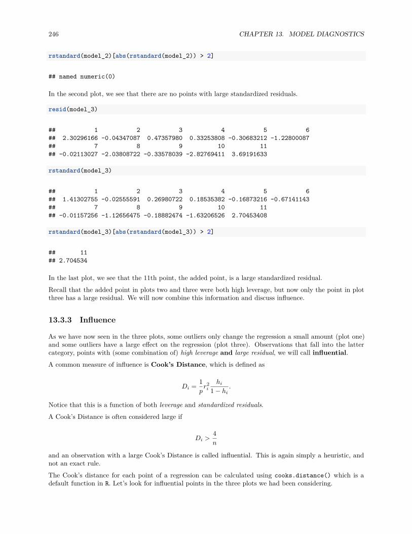
246 CHAPTER 13. MODEL DIAGNOSTICS
rstandard(model_2)[abs(rstandard(model_2)) > 2]
## named numeric(0)
In the second plot, we see that there are no points with large standardized residuals.
resid(model_3)
## 1 2 3 4 5 6## 2.30296166 -0.04347087 0.47357980 0.33253808 -0.30683212 -1.22800087## 7 8 9 10 11## -0.02113027 -2.03808722 -0.33578039 -2.82769411 3.69191633
rstandard(model_3)
## 1 2 3 4 5 6## 1.41302755 -0.02555591 0.26980722 0.18535382 -0.16873216 -0.67141143## 7 8 9 10 11## -0.01157256 -1.12656475 -0.18882474 -1.63206526 2.70453408
rstandard(model_3)[abs(rstandard(model_3)) > 2]
## 11## 2.704534
In the last plot, we see that the 11th point, the added point, is a large standardized residual.Recall that the added point in plots two and three were both high leverage, but now only the point in plotthree has a large residual. We will now combine this information and discuss influence.
13.3.3 Influence
As we have now seen in the three plots, some outliers only change the regression a small amount (plot one)and some outliers have a large effect on the regression (plot three). Observations that fall into the lattercategory, points with (some combination of) high leverage and large residual, we will call influential.A common measure of influence is Cook’s Distance, which is defined as
Di = 1p
r2i
hi
1 − hi.
Notice that this is a function of both leverage and standardized residuals.A Cook’s Distance is often considered large if
Di >4n
and an observation with a large Cook’s Distance is called influential. This is again simply a heuristic, andnot an exact rule.The Cook’s distance for each point of a regression can be calculated using cooks.distance() which is adefault function in R. Let’s look for influential points in the three plots we had been considering.
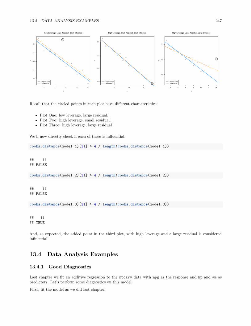
13.4. DATA ANALYSIS EXAMPLES 247
2 4 6 8 10
24
68
10Low Leverage, Large Residual, Small Influence
x
y
Original DataAdded Point
5 10 15
-50
510
High Leverage, Small Residual, Small Influence
x
y
Original DataAdded Point
2 4 6 8 10 12 14
05
10
High Leverage, Large Residual, Large Influence
x
y
Original DataAdded Point
Recall that the circled points in each plot have different characteristics:
• Plot One: low leverage, large residual.• Plot Two: high leverage, small residual.• Plot Three: high leverage, large residual.
We’ll now directly check if each of these is influential.
cooks.distance(model_1)[11] > 4 / length(cooks.distance(model_1))
## 11## FALSE
cooks.distance(model_2)[11] > 4 / length(cooks.distance(model_2))
## 11## FALSE
cooks.distance(model_3)[11] > 4 / length(cooks.distance(model_3))
## 11## TRUE
And, as expected, the added point in the third plot, with high leverage and a large residual is consideredinfluential!
13.4 Data Analysis Examples
13.4.1 Good Diagnostics
Last chapter we fit an additive regression to the mtcars data with mpg as the response and hp and am aspredictors. Let’s perform some diagnostics on this model.
First, fit the model as we did last chapter.
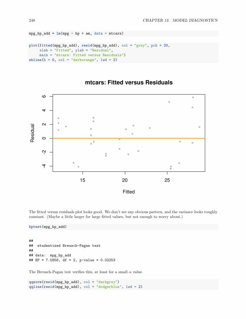
248 CHAPTER 13. MODEL DIAGNOSTICS
mpg_hp_add = lm(mpg ~ hp + am, data = mtcars)
plot(fitted(mpg_hp_add), resid(mpg_hp_add), col = "grey", pch = 20,xlab = "Fitted", ylab = "Residual",main = "mtcars: Fitted versus Residuals")
abline(h = 0, col = "darkorange", lwd = 2)
15 20 25
-4-2
02
46
mtcars: Fitted versus Residuals
Fitted
Res
idua
l
The fitted versus residuals plot looks good. We don’t see any obvious pattern, and the variance looks roughlyconstant. (Maybe a little larger for large fitted values, but not enough to worry about.)
bptest(mpg_hp_add)
#### studentized Breusch-Pagan test#### data: mpg_hp_add## BP = 7.5858, df = 2, p-value = 0.02253
The Breusch-Pagan test verifies this, at least for a small α value.
qqnorm(resid(mpg_hp_add), col = "darkgrey")qqline(resid(mpg_hp_add), col = "dodgerblue", lwd = 2)

13.4. DATA ANALYSIS EXAMPLES 249
-2 -1 0 1 2
-4-2
02
46
Normal Q-Q Plot
Theoretical Quantiles
Sam
ple
Qua
ntile
s
The Q-Q plot looks extremely good and the Shapiro-Wilk test agrees.
shapiro.test(resid(mpg_hp_add))
#### Shapiro-Wilk normality test#### data: resid(mpg_hp_add)## W = 0.96485, p-value = 0.3706
sum(hatvalues(mpg_hp_add) > 2 * mean(hatvalues(mpg_hp_add)))
## [1] 2
We see that there are two points of large leverage.
sum(abs(rstandard(mpg_hp_add)) > 2)
## [1] 1
There is also one point with a large residual. Do these result in any points that are considered influential?

250 CHAPTER 13. MODEL DIAGNOSTICS
cd_mpg_hp_add = cooks.distance(mpg_hp_add)sum(cd_mpg_hp_add > 4 / length(cd_mpg_hp_add))
## [1] 2
large_cd_mpg = cd_mpg_hp_add > 4 / length(cd_mpg_hp_add)cd_mpg_hp_add[large_cd_mpg]
## Toyota Corolla Maserati Bora## 0.1772555 0.3447994
We find two influential points. Interestingly, they are very different cars.
coef(mpg_hp_add)
## (Intercept) hp am## 26.5849137 -0.0588878 5.2770853
Since the diagnostics looked good, there isn’t much need to worry about these two points, but let’s see howmuch the coefficients change if we remove them.
mpg_hp_add_fix = lm(mpg ~ hp + am,data = mtcars,subset = cd_mpg_hp_add <= 4 / length(cd_mpg_hp_add))
coef(mpg_hp_add_fix)
## (Intercept) hp am## 27.22190933 -0.06286249 4.29765867
It seems there isn’t much of a change in the coefficients as a results of removing the supposed influentialpoints. Notice we did not create a new dataset to accomplish this. We instead used the subset argumentto lm(). Think about what the code cd_mpg_hp_add <= 4 / length(cd_mpg_hp_add) does here.
par(mfrow = c(2, 2))plot(mpg_hp_add)
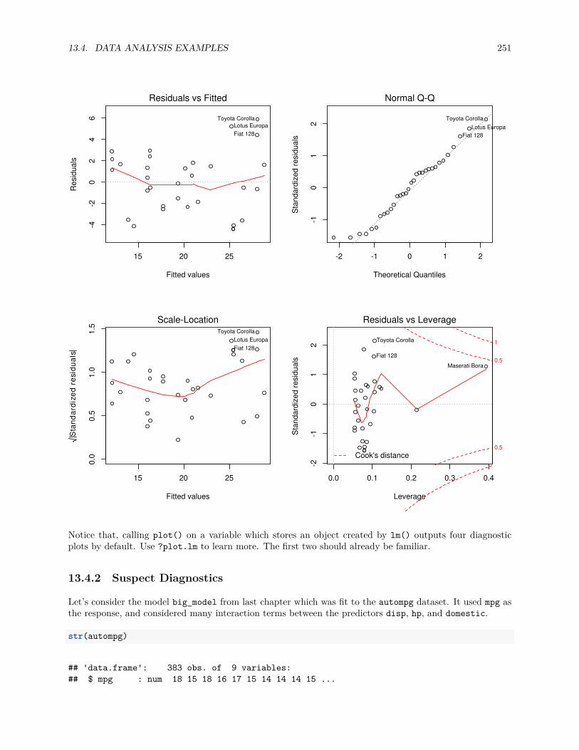
13.4. DATA ANALYSIS EXAMPLES 251
15 20 25
-4-2
02
46
Fitted values
Res
idua
ls
Residuals vs Fitted
Toyota CorollaLotus EuropaFiat 128
-2 -1 0 1 2
-10
12
Theoretical Quantiles
Sta
ndar
dize
d re
sidu
als
Normal Q-Q
Toyota CorollaLotus Europa
Fiat 128
15 20 25
0.0
0.5
1.0
1.5
Fitted values
Sta
ndar
dize
d re
sidu
als
Scale-LocationToyota Corolla
Lotus EuropaFiat 128
0.0 0.1 0.2 0.3 0.4
-2-1
01
2
Leverage
Sta
ndar
dize
d re
sidu
als
Cook's distance0.5
0.5
1
Residuals vs Leverage
Maserati Bora
Toyota Corolla
Fiat 128
Notice that, calling plot() on a variable which stores an object created by lm() outputs four diagnosticplots by default. Use ?plot.lm to learn more. The first two should already be familiar.
13.4.2 Suspect Diagnostics
Let’s consider the model big_model from last chapter which was fit to the autompg dataset. It used mpg asthe response, and considered many interaction terms between the predictors disp, hp, and domestic.
str(autompg)
## 'data.frame': 383 obs. of 9 variables:## $ mpg : num 18 15 18 16 17 15 14 14 14 15 ...
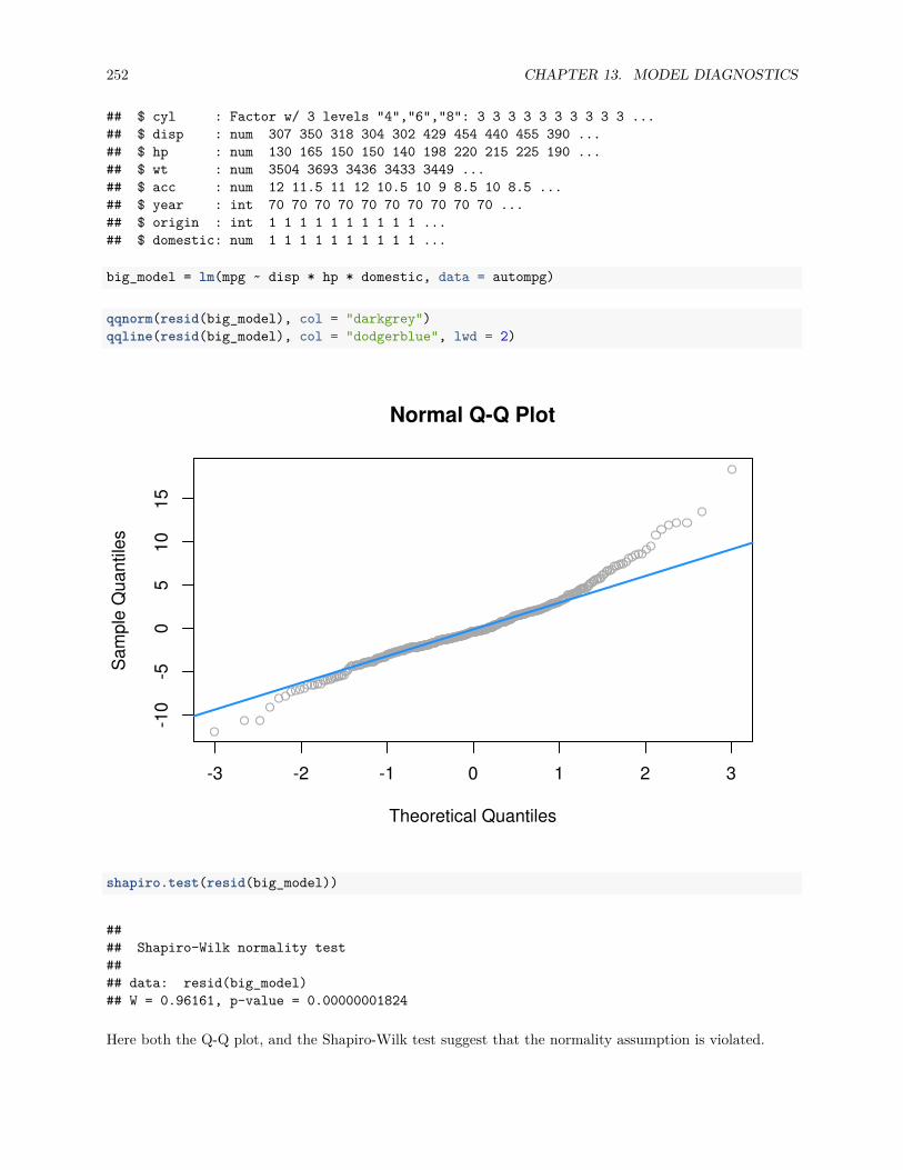
252 CHAPTER 13. MODEL DIAGNOSTICS
## $ cyl : Factor w/ 3 levels "4","6","8": 3 3 3 3 3 3 3 3 3 3 ...## $ disp : num 307 350 318 304 302 429 454 440 455 390 ...## $ hp : num 130 165 150 150 140 198 220 215 225 190 ...## $ wt : num 3504 3693 3436 3433 3449 ...## $ acc : num 12 11.5 11 12 10.5 10 9 8.5 10 8.5 ...## $ year : int 70 70 70 70 70 70 70 70 70 70 ...## $ origin : int 1 1 1 1 1 1 1 1 1 1 ...## $ domestic: num 1 1 1 1 1 1 1 1 1 1 ...
big_model = lm(mpg ~ disp * hp * domestic, data = autompg)
qqnorm(resid(big_model), col = "darkgrey")qqline(resid(big_model), col = "dodgerblue", lwd = 2)
-3 -2 -1 0 1 2 3
-10
-50
510
15
Normal Q-Q Plot
Theoretical Quantiles
Sam
ple
Qua
ntile
s
shapiro.test(resid(big_model))
#### Shapiro-Wilk normality test#### data: resid(big_model)## W = 0.96161, p-value = 0.00000001824
Here both the Q-Q plot, and the Shapiro-Wilk test suggest that the normality assumption is violated.
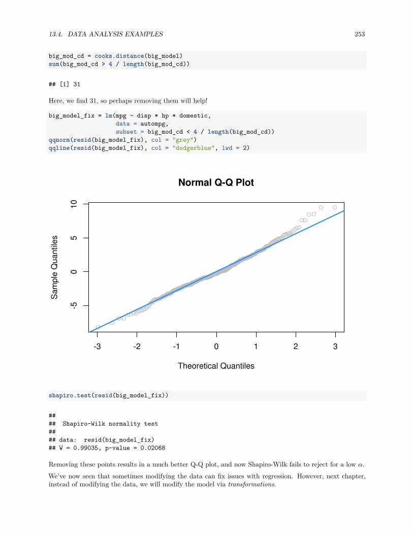
13.4. DATA ANALYSIS EXAMPLES 253
big_mod_cd = cooks.distance(big_model)sum(big_mod_cd > 4 / length(big_mod_cd))
## [1] 31
Here, we find 31, so perhaps removing them will help!
big_model_fix = lm(mpg ~ disp * hp * domestic,data = autompg,subset = big_mod_cd < 4 / length(big_mod_cd))
qqnorm(resid(big_model_fix), col = "grey")qqline(resid(big_model_fix), col = "dodgerblue", lwd = 2)
-3 -2 -1 0 1 2 3
-50
510
Normal Q-Q Plot
Theoretical Quantiles
Sam
ple
Qua
ntile
s
shapiro.test(resid(big_model_fix))
#### Shapiro-Wilk normality test#### data: resid(big_model_fix)## W = 0.99035, p-value = 0.02068
Removing these points results in a much better Q-Q plot, and now Shapiro-Wilk fails to reject for a low α.We’ve now seen that sometimes modifying the data can fix issues with regression. However, next chapter,instead of modifying the data, we will modify the model via transformations.

254 CHAPTER 13. MODEL DIAGNOSTICS

Chapter 14
Transformations
“Give me a lever long enough and a fulcrum on which to place it, and I shall move the world.”
— Archimedes
Please note: some data currently used in this chapter was used, changed, and passed around over theyears in STAT 420 at UIUC. Its original sources, if they exist, are at this time unknown to the author. Asa result, they should only be considered for use with STAT 420. Going forward they will likely be replacedwith alternative sourceable data that illustrates the same concepts. At the end of this chapter you can findcode seen in videos for Week 8 for STAT 420 in the MCS-DS program. It is currently in the process of beingmerged into the narrative of this chapter.
After reading this chapter you will be able to:
• Understand the concept of a variance stabilizing transformation.• Use transformations of the response to improve regression models.• Use polynomial terms as predictors to fit more flexible regression models.
Last chapter we checked the assumptions of regression models and looked at ways to diagnose possible issues.This chapter we will use transformations of both response and predictor variables in order to correct issueswith model diagnostics, and to also potentially simply make a model fit data better.
14.1 Response Transformation
Let’s look at some (fictional) salary data from the (fictional) company Initech. We will try to model salaryas a function of years of experience. The data can be found in initech.csv.
initech = read.csv("data/initech.csv")
plot(salary ~ years, data = initech, col = "grey", pch = 20, cex = 1.5,main = "Salaries at Initech, By Seniority")
255
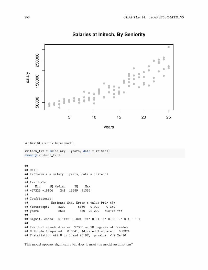
256 CHAPTER 14. TRANSFORMATIONS
5 10 15 20 25
5000
015
0000
2500
00Salaries at Initech, By Seniority
years
sala
ry
We first fit a simple linear model.
initech_fit = lm(salary ~ years, data = initech)summary(initech_fit)
#### Call:## lm(formula = salary ~ years, data = initech)#### Residuals:## Min 1Q Median 3Q Max## -57225 -18104 241 15589 91332#### Coefficients:## Estimate Std. Error t value Pr(>|t|)## (Intercept) 5302 5750 0.922 0.359## years 8637 389 22.200 <2e-16 ***## ---## Signif. codes: 0 '***' 0.001 '**' 0.01 '*' 0.05 '.' 0.1 ' ' 1#### Residual standard error: 27360 on 98 degrees of freedom## Multiple R-squared: 0.8341, Adjusted R-squared: 0.8324## F-statistic: 492.8 on 1 and 98 DF, p-value: < 2.2e-16
This model appears significant, but does it meet the model assumptions?
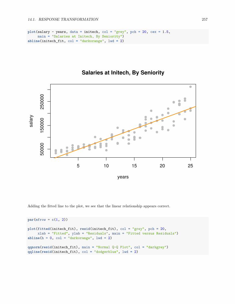
14.1. RESPONSE TRANSFORMATION 257
plot(salary ~ years, data = initech, col = "grey", pch = 20, cex = 1.5,main = "Salaries at Initech, By Seniority")
abline(initech_fit, col = "darkorange", lwd = 2)
5 10 15 20 25
5000
015
0000
2500
00
Salaries at Initech, By Seniority
years
sala
ry
Adding the fitted line to the plot, we see that the linear relationship appears correct.
par(mfrow = c(1, 2))
plot(fitted(initech_fit), resid(initech_fit), col = "grey", pch = 20,xlab = "Fitted", ylab = "Residuals", main = "Fitted versus Residuals")
abline(h = 0, col = "darkorange", lwd = 2)
qqnorm(resid(initech_fit), main = "Normal Q-Q Plot", col = "darkgrey")qqline(resid(initech_fit), col = "dodgerblue", lwd = 2)
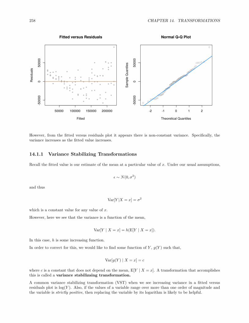
258 CHAPTER 14. TRANSFORMATIONS
50000 100000 150000 200000
-500
000
5000
0Fitted versus Residuals
Fitted
Res
idua
ls
-2 -1 0 1 2
-500
000
5000
0
Normal Q-Q Plot
Theoretical Quantiles
Sam
ple
Qua
ntile
s
However, from the fitted versus residuals plot it appears there is non-constant variance. Specifically, thevariance increases as the fitted value increases.
14.1.1 Variance Stabilizing Transformations
Recall the fitted value is our estimate of the mean at a particular value of x. Under our usual assumptions,
ϵ ∼ N(0, σ2)
and thus
Var[Y |X = x] = σ2
which is a constant value for any value of x.
However, here we see that the variance is a function of the mean,
Var[Y | X = x] = h(E[Y | X = x]).
In this case, h is some increasing function.
In order to correct for this, we would like to find some function of Y , g(Y ) such that,
Var[g(Y ) | X = x] = c
where c is a constant that does not depend on the mean, E[Y | X = x]. A transformation that accomplishesthis is called a variance stabilizaing transformation.
A common variance stabilizing transformation (VST) when we see increasing variance in a fitted versusresiduals plot is log(Y ). Also, if the values of a variable range over more than one order of magnitude andthe variable is strictly positive, then replacing the variable by its logarithm is likely to be helpful.
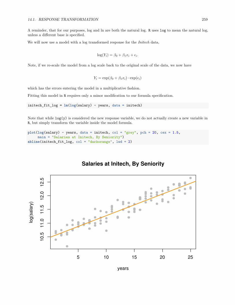
14.1. RESPONSE TRANSFORMATION 259
A reminder, that for our purposes, log and ln are both the natural log. R uses log to mean the natural log,unless a different base is specified.
We will now use a model with a log transformed response for the Initech data,
log(Yi) = β0 + β1xi + ϵi.
Note, if we re-scale the model from a log scale back to the original scale of the data, we now have
Yi = exp(β0 + β1xi) · exp(ϵi)
which has the errors entering the model in a multiplicative fashion.
Fitting this model in R requires only a minor modification to our formula specification.
initech_fit_log = lm(log(salary) ~ years, data = initech)
Note that while log(y) is considered the new response variable, we do not actually create a new variable inR, but simply transform the variable inside the model formula.
plot(log(salary) ~ years, data = initech, col = "grey", pch = 20, cex = 1.5,main = "Salaries at Initech, By Seniority")
abline(initech_fit_log, col = "darkorange", lwd = 2)
5 10 15 20 25
10.5
11.0
11.5
12.0
12.5
Salaries at Initech, By Seniority
years
log(
sala
ry)
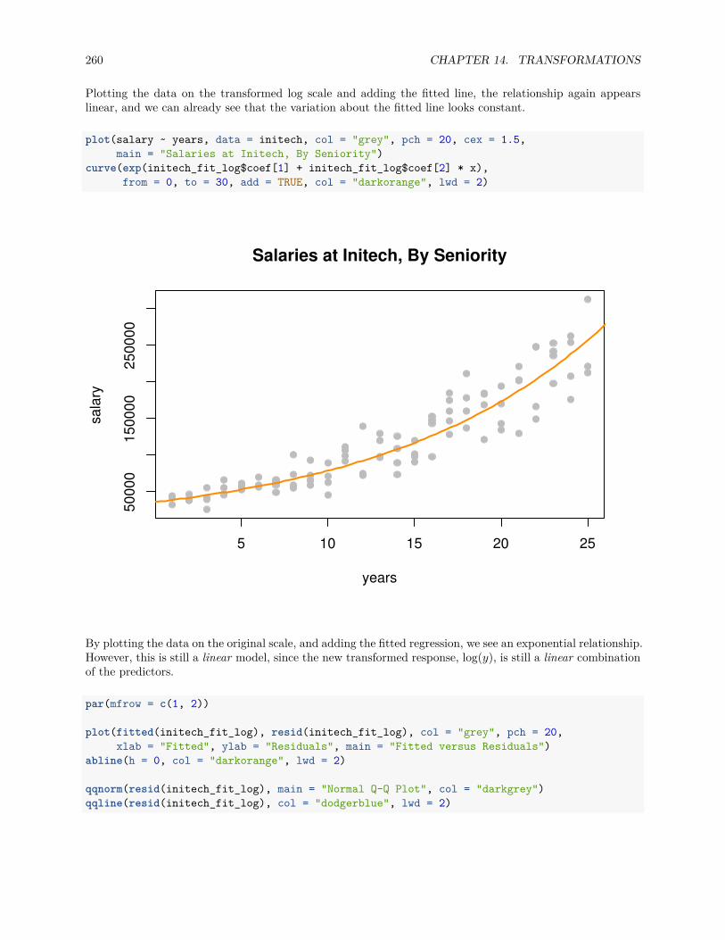
260 CHAPTER 14. TRANSFORMATIONS
Plotting the data on the transformed log scale and adding the fitted line, the relationship again appearslinear, and we can already see that the variation about the fitted line looks constant.
plot(salary ~ years, data = initech, col = "grey", pch = 20, cex = 1.5,main = "Salaries at Initech, By Seniority")
curve(exp(initech_fit_log$coef[1] + initech_fit_log$coef[2] * x),from = 0, to = 30, add = TRUE, col = "darkorange", lwd = 2)
5 10 15 20 25
5000
015
0000
2500
00
Salaries at Initech, By Seniority
years
sala
ry
By plotting the data on the original scale, and adding the fitted regression, we see an exponential relationship.However, this is still a linear model, since the new transformed response, log(y), is still a linear combinationof the predictors.
par(mfrow = c(1, 2))
plot(fitted(initech_fit_log), resid(initech_fit_log), col = "grey", pch = 20,xlab = "Fitted", ylab = "Residuals", main = "Fitted versus Residuals")
abline(h = 0, col = "darkorange", lwd = 2)
qqnorm(resid(initech_fit_log), main = "Normal Q-Q Plot", col = "darkgrey")qqline(resid(initech_fit_log), col = "dodgerblue", lwd = 2)
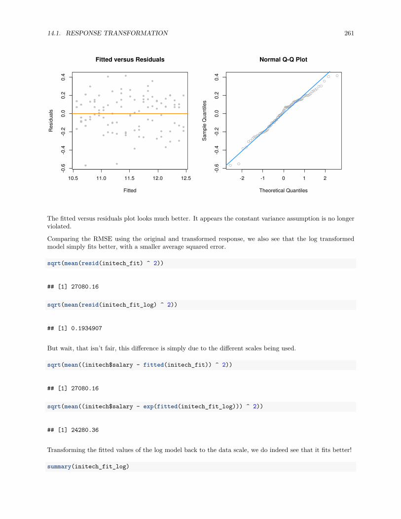
14.1. RESPONSE TRANSFORMATION 261
10.5 11.0 11.5 12.0 12.5
-0.6
-0.4
-0.2
0.0
0.2
0.4
Fitted versus Residuals
Fitted
Res
idua
ls
-2 -1 0 1 2
-0.6
-0.4
-0.2
0.0
0.2
0.4
Normal Q-Q Plot
Theoretical Quantiles
Sam
ple
Qua
ntile
s
The fitted versus residuals plot looks much better. It appears the constant variance assumption is no longerviolated.
Comparing the RMSE using the original and transformed response, we also see that the log transformedmodel simply fits better, with a smaller average squared error.
sqrt(mean(resid(initech_fit) ^ 2))
## [1] 27080.16
sqrt(mean(resid(initech_fit_log) ^ 2))
## [1] 0.1934907
But wait, that isn’t fair, this difference is simply due to the different scales being used.
sqrt(mean((initech$salary - fitted(initech_fit)) ^ 2))
## [1] 27080.16
sqrt(mean((initech$salary - exp(fitted(initech_fit_log))) ^ 2))
## [1] 24280.36
Transforming the fitted values of the log model back to the data scale, we do indeed see that it fits better!
summary(initech_fit_log)
262 CHAPTER 14. TRANSFORMATIONS
#### Call:## lm(formula = log(salary) ~ years, data = initech)#### Residuals:## Min 1Q Median 3Q Max## -0.57022 -0.13560 0.03048 0.14157 0.41366#### Coefficients:## Estimate Std. Error t value Pr(>|t|)## (Intercept) 10.48381 0.04108 255.18 <2e-16 ***## years 0.07888 0.00278 28.38 <2e-16 ***## ---## Signif. codes: 0 '***' 0.001 '**' 0.01 '*' 0.05 '.' 0.1 ' ' 1#### Residual standard error: 0.1955 on 98 degrees of freedom## Multiple R-squared: 0.8915, Adjusted R-squared: 0.8904## F-statistic: 805.2 on 1 and 98 DF, p-value: < 2.2e-16
Again, the transformed response is a linear combination of the predictors,
log(y(x)) = β0 + β1x = 10.484 + 0.079x.
But now, if we re-scale the data from a log scale back to the original scale of the data, we now have
y(x) = exp(β0) exp(β1x) = exp(10.484) exp(0.079x).
We see that for every one additional year of experience, average salary increases exp(0.079) = 1.0822 times.We are now multiplying, not adding.
While using a log transform is possibly the most common response variable transformation, many othersexist. We will now consider a family of transformations and choose the best from among them, which includesthe log transform.
14.1.2 Box-Cox Transformations
The Box-Cox method considers a family of transformations on strictly positive response variables,
gλ(y) =
yλ − 1
λλ = 0
log(y) λ = 0
The λ parameter is chosen by numerically maximizing the log-likelihood,
L(λ) = −n
2log(RSSλ/n) + (λ − 1)
∑log(yi).
A 100(1 − α)% confidence interval for λ is,
{λ : L(λ) > L(λ) − 1
2χ2
1,α
}
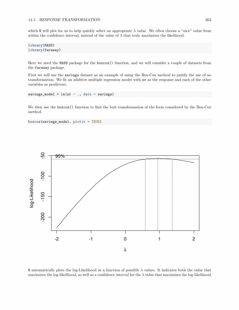
14.1. RESPONSE TRANSFORMATION 263
which R will plot for us to help quickly select an appropriate λ value. We often choose a “nice” value fromwithin the confidence interval, instead of the value of λ that truly maximizes the likelihood.
library(MASS)library(faraway)
Here we need the MASS package for the boxcox() function, and we will consider a couple of datasets fromthe faraway package.
First we will use the savings dataset as an example of using the Box-Cox method to justify the use of notransformation. We fit an additive multiple regression model with sr as the response and each of the othervariables as predictors.
savings_model = lm(sr ~ ., data = savings)
We then use the boxcox() function to find the best transformation of the form considered by the Box-Coxmethod.
boxcox(savings_model, plotit = TRUE)
-2 -1 0 1 2
-200
-150
-100
-50
λ
log-
Like
lihoo
d
95%
R automatically plots the log-Likelihood as a function of possible λ values. It indicates both the value thatmaximizes the log-likelihood, as well as a confidence interval for the λ value that maximizes the log-likelihood.
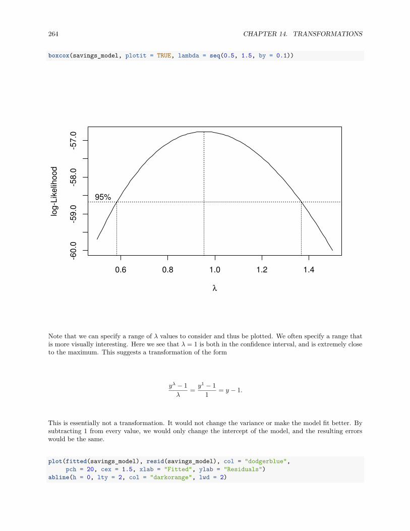
264 CHAPTER 14. TRANSFORMATIONS
boxcox(savings_model, plotit = TRUE, lambda = seq(0.5, 1.5, by = 0.1))
0.6 0.8 1.0 1.2 1.4
-60.
0-5
9.0
-58.
0-5
7.0
λ
log-
Like
lihoo
d
95%
Note that we can specify a range of λ values to consider and thus be plotted. We often specify a range thatis more visually interesting. Here we see that λ = 1 is both in the confidence interval, and is extremely closeto the maximum. This suggests a transformation of the form
yλ − 1λ
= y1 − 11
= y − 1.
This is essentially not a transformation. It would not change the variance or make the model fit better. Bysubtracting 1 from every value, we would only change the intercept of the model, and the resulting errorswould be the same.
plot(fitted(savings_model), resid(savings_model), col = "dodgerblue",pch = 20, cex = 1.5, xlab = "Fitted", ylab = "Residuals")
abline(h = 0, lty = 2, col = "darkorange", lwd = 2)
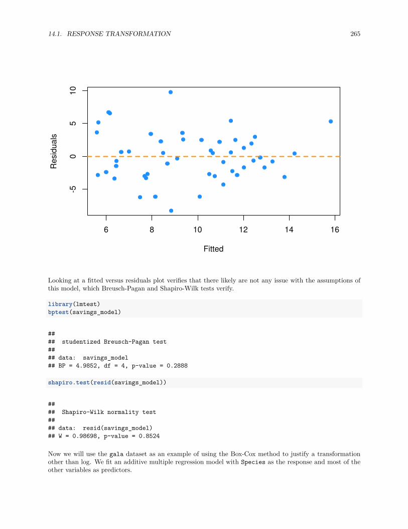
14.1. RESPONSE TRANSFORMATION 265
6 8 10 12 14 16
-50
510
Fitted
Res
idua
ls
Looking at a fitted versus residuals plot verifies that there likely are not any issue with the assumptions ofthis model, which Breusch-Pagan and Shapiro-Wilk tests verify.
library(lmtest)bptest(savings_model)
#### studentized Breusch-Pagan test#### data: savings_model## BP = 4.9852, df = 4, p-value = 0.2888
shapiro.test(resid(savings_model))
#### Shapiro-Wilk normality test#### data: resid(savings_model)## W = 0.98698, p-value = 0.8524
Now we will use the gala dataset as an example of using the Box-Cox method to justify a transformationother than log. We fit an additive multiple regression model with Species as the response and most of theother variables as predictors.
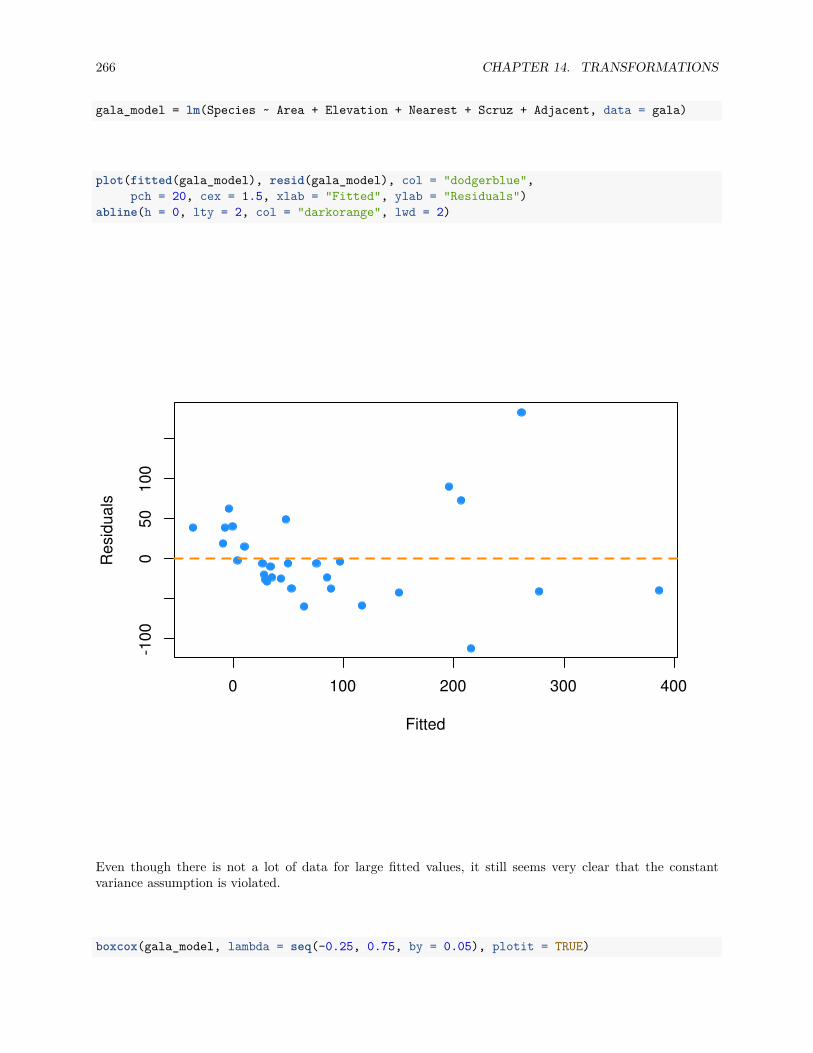
266 CHAPTER 14. TRANSFORMATIONS
gala_model = lm(Species ~ Area + Elevation + Nearest + Scruz + Adjacent, data = gala)
plot(fitted(gala_model), resid(gala_model), col = "dodgerblue",pch = 20, cex = 1.5, xlab = "Fitted", ylab = "Residuals")
abline(h = 0, lty = 2, col = "darkorange", lwd = 2)
0 100 200 300 400
-100
050
100
Fitted
Res
idua
ls
Even though there is not a lot of data for large fitted values, it still seems very clear that the constantvariance assumption is violated.
boxcox(gala_model, lambda = seq(-0.25, 0.75, by = 0.05), plotit = TRUE)
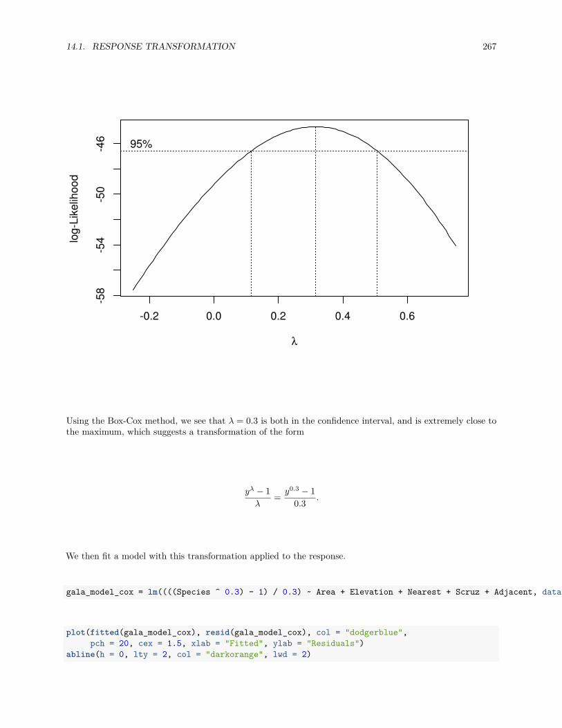
14.1. RESPONSE TRANSFORMATION 267
-0.2 0.0 0.2 0.4 0.6
-58
-54
-50
-46
λ
log-
Like
lihoo
d
95%
Using the Box-Cox method, we see that λ = 0.3 is both in the confidence interval, and is extremely close tothe maximum, which suggests a transformation of the form
yλ − 1λ
= y0.3 − 10.3
.
We then fit a model with this transformation applied to the response.
gala_model_cox = lm((((Species ^ 0.3) - 1) / 0.3) ~ Area + Elevation + Nearest + Scruz + Adjacent, data = gala)
plot(fitted(gala_model_cox), resid(gala_model_cox), col = "dodgerblue",pch = 20, cex = 1.5, xlab = "Fitted", ylab = "Residuals")
abline(h = 0, lty = 2, col = "darkorange", lwd = 2)
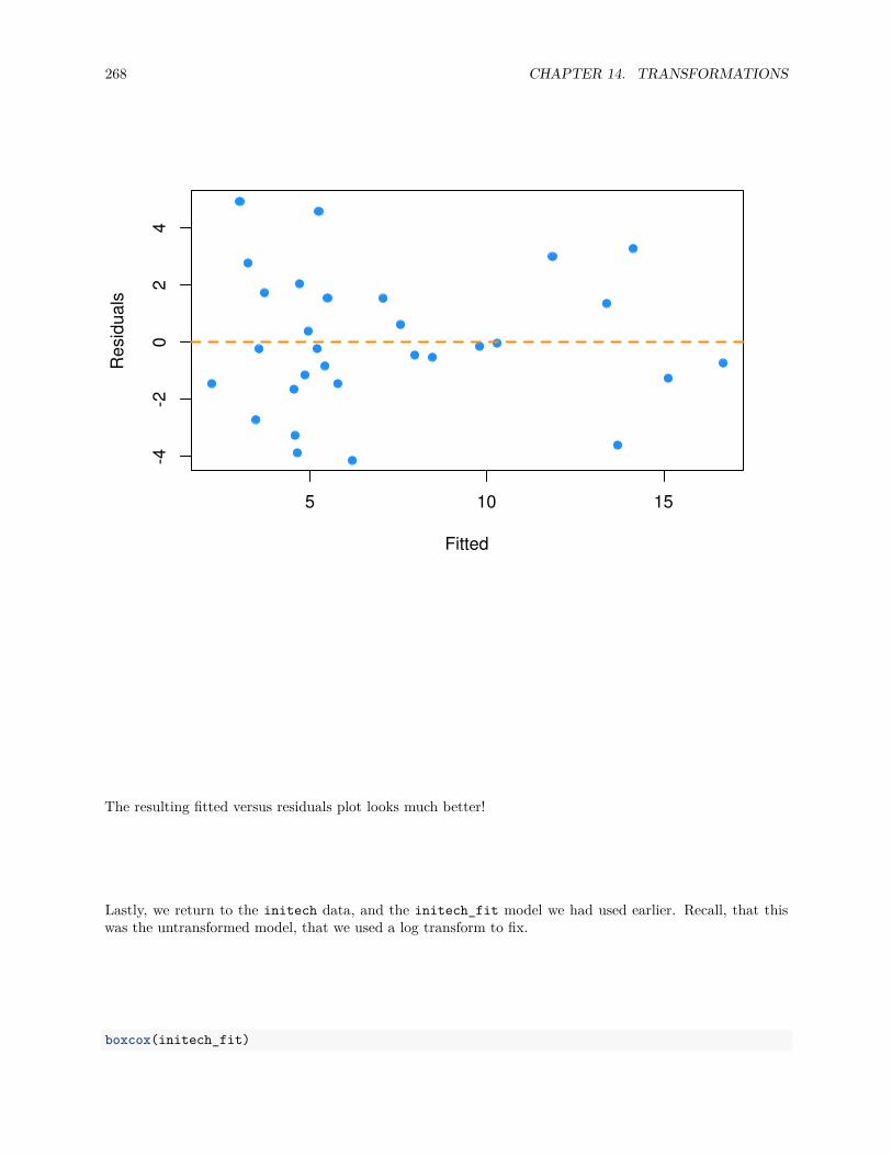
268 CHAPTER 14. TRANSFORMATIONS
5 10 15
-4-2
02
4
Fitted
Res
idua
ls
The resulting fitted versus residuals plot looks much better!
Lastly, we return to the initech data, and the initech_fit model we had used earlier. Recall, that thiswas the untransformed model, that we used a log transform to fix.
boxcox(initech_fit)
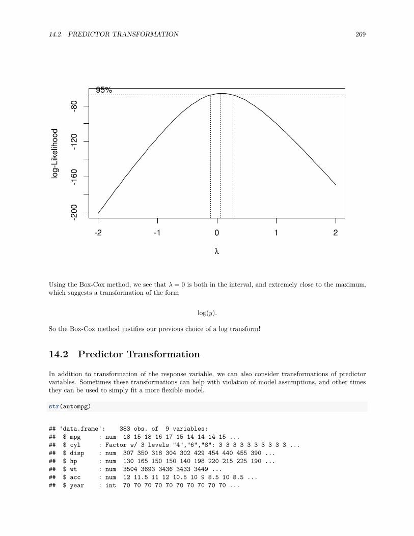
14.2. PREDICTOR TRANSFORMATION 269
-2 -1 0 1 2
-200
-160
-120
-80
λ
log-
Like
lihoo
d
95%
Using the Box-Cox method, we see that λ = 0 is both in the interval, and extremely close to the maximum,which suggests a transformation of the form
log(y).
So the Box-Cox method justifies our previous choice of a log transform!
14.2 Predictor Transformation
In addition to transformation of the response variable, we can also consider transformations of predictorvariables. Sometimes these transformations can help with violation of model assumptions, and other timesthey can be used to simply fit a more flexible model.
str(autompg)
## 'data.frame': 383 obs. of 9 variables:## $ mpg : num 18 15 18 16 17 15 14 14 14 15 ...## $ cyl : Factor w/ 3 levels "4","6","8": 3 3 3 3 3 3 3 3 3 3 ...## $ disp : num 307 350 318 304 302 429 454 440 455 390 ...## $ hp : num 130 165 150 150 140 198 220 215 225 190 ...## $ wt : num 3504 3693 3436 3433 3449 ...## $ acc : num 12 11.5 11 12 10.5 10 9 8.5 10 8.5 ...## $ year : int 70 70 70 70 70 70 70 70 70 70 ...
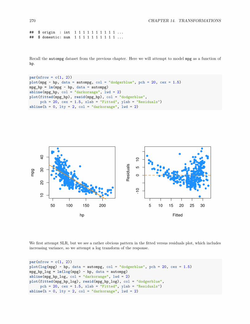
270 CHAPTER 14. TRANSFORMATIONS
## $ origin : int 1 1 1 1 1 1 1 1 1 1 ...## $ domestic: num 1 1 1 1 1 1 1 1 1 1 ...
Recall the autompg dataset from the previous chapter. Here we will attempt to model mpg as a function ofhp.
par(mfrow = c(1, 2))plot(mpg ~ hp, data = autompg, col = "dodgerblue", pch = 20, cex = 1.5)mpg_hp = lm(mpg ~ hp, data = autompg)abline(mpg_hp, col = "darkorange", lwd = 2)plot(fitted(mpg_hp), resid(mpg_hp), col = "dodgerblue",
pch = 20, cex = 1.5, xlab = "Fitted", ylab = "Residuals")abline(h = 0, lty = 2, col = "darkorange", lwd = 2)
50 100 150 200
1020
3040
hp
mpg
5 10 15 20 25 30
-10
05
10
Fitted
Res
idua
ls
We first attempt SLR, but we see a rather obvious pattern in the fitted versus residuals plot, which includesincreasing variance, so we attempt a log transform of the response.
par(mfrow = c(1, 2))plot(log(mpg) ~ hp, data = autompg, col = "dodgerblue", pch = 20, cex = 1.5)mpg_hp_log = lm(log(mpg) ~ hp, data = autompg)abline(mpg_hp_log, col = "darkorange", lwd = 2)plot(fitted(mpg_hp_log), resid(mpg_hp_log), col = "dodgerblue",
pch = 20, cex = 1.5, xlab = "Fitted", ylab = "Residuals")abline(h = 0, lty = 2, col = "darkorange", lwd = 2)
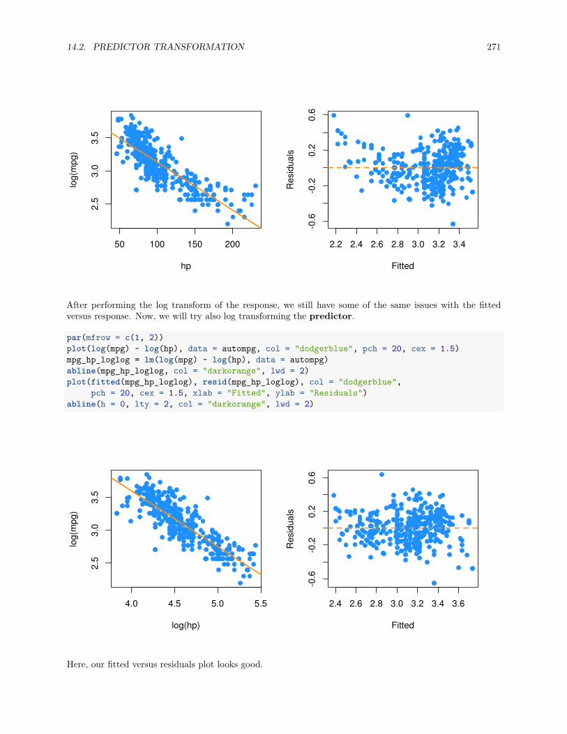
14.2. PREDICTOR TRANSFORMATION 271
50 100 150 200
2.5
3.0
3.5
hp
log(
mpg
)
2.2 2.4 2.6 2.8 3.0 3.2 3.4
-0.6
-0.2
0.2
0.6
Fitted
Res
idua
ls
After performing the log transform of the response, we still have some of the same issues with the fittedversus response. Now, we will try also log transforming the predictor.
par(mfrow = c(1, 2))plot(log(mpg) ~ log(hp), data = autompg, col = "dodgerblue", pch = 20, cex = 1.5)mpg_hp_loglog = lm(log(mpg) ~ log(hp), data = autompg)abline(mpg_hp_loglog, col = "darkorange", lwd = 2)plot(fitted(mpg_hp_loglog), resid(mpg_hp_loglog), col = "dodgerblue",
pch = 20, cex = 1.5, xlab = "Fitted", ylab = "Residuals")abline(h = 0, lty = 2, col = "darkorange", lwd = 2)
4.0 4.5 5.0 5.5
2.5
3.0
3.5
log(hp)
log(
mpg
)
2.4 2.6 2.8 3.0 3.2 3.4 3.6
-0.6
-0.2
0.2
0.6
Fitted
Res
idua
ls
Here, our fitted versus residuals plot looks good.
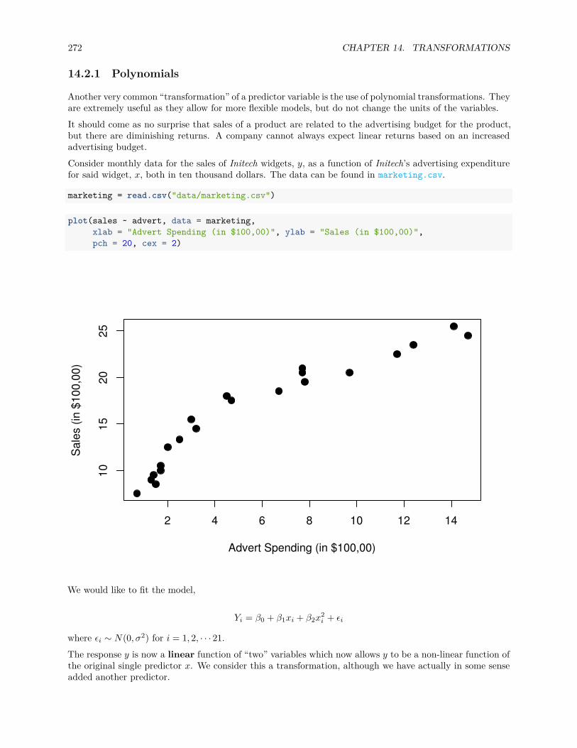
272 CHAPTER 14. TRANSFORMATIONS
14.2.1 Polynomials
Another very common “transformation” of a predictor variable is the use of polynomial transformations. Theyare extremely useful as they allow for more flexible models, but do not change the units of the variables.It should come as no surprise that sales of a product are related to the advertising budget for the product,but there are diminishing returns. A company cannot always expect linear returns based on an increasedadvertising budget.Consider monthly data for the sales of Initech widgets, y, as a function of Initech’s advertising expenditurefor said widget, x, both in ten thousand dollars. The data can be found in marketing.csv.
marketing = read.csv("data/marketing.csv")
plot(sales ~ advert, data = marketing,xlab = "Advert Spending (in $100,00)", ylab = "Sales (in $100,00)",pch = 20, cex = 2)
2 4 6 8 10 12 14
1015
2025
Advert Spending (in $100,00)
Sal
es (i
n $1
00,0
0)
We would like to fit the model,
Yi = β0 + β1xi + β2x2i + ϵi
where ϵi ∼ N(0, σ2) for i = 1, 2, · · · 21.
The response y is now a linear function of “two” variables which now allows y to be a non-linear function ofthe original single predictor x. We consider this a transformation, although we have actually in some senseadded another predictor.
14.2. PREDICTOR TRANSFORMATION 273
Thus, our X matrix is,
1 x1 x21
1 x2 x22
1 x3 x23
......
...1 xn x2
n
We can then proceed to fit the model as we have in the past for multiple linear regression.
β =(X⊤X
)−1X⊤y.
Our estimates will have the usual properties. The mean is still
E[β] = β,
and variance
Var[β] = σ2 (X⊤X)−1
.
We also maintain the same distributional results
βj ∼ N(βj , σ2Cjj
).
mark_mod = lm(sales ~ advert, data = marketing)summary(mark_mod)
#### Call:## lm(formula = sales ~ advert, data = marketing)#### Residuals:## Min 1Q Median 3Q Max## -2.7845 -1.4762 -0.5103 1.2361 3.1869#### Coefficients:## Estimate Std. Error t value Pr(>|t|)## (Intercept) 9.4502 0.6806 13.88 2.13e-11 ***## advert 1.1918 0.0937 12.72 9.65e-11 ***## ---## Signif. codes: 0 '***' 0.001 '**' 0.01 '*' 0.05 '.' 0.1 ' ' 1#### Residual standard error: 1.907 on 19 degrees of freedom## Multiple R-squared: 0.8949, Adjusted R-squared: 0.8894## F-statistic: 161.8 on 1 and 19 DF, p-value: 9.646e-11
While the SLR model is significant, the fitted versus residuals plot would have a very clear pattern.
274 CHAPTER 14. TRANSFORMATIONS
mark_mod_poly2 = lm(sales ~ advert + I(advert ^ 2), data = marketing)summary(mark_mod_poly2)
#### Call:## lm(formula = sales ~ advert + I(advert^2), data = marketing)#### Residuals:## Min 1Q Median 3Q Max## -1.9175 -0.8333 -0.1948 0.9292 2.1385#### Coefficients:## Estimate Std. Error t value Pr(>|t|)## (Intercept) 6.76161 0.67219 10.059 8.16e-09 ***## advert 2.46231 0.24830 9.917 1.02e-08 ***## I(advert^2) -0.08745 0.01658 -5.275 5.14e-05 ***## ---## Signif. codes: 0 '***' 0.001 '**' 0.01 '*' 0.05 '.' 0.1 ' ' 1#### Residual standard error: 1.228 on 18 degrees of freedom## Multiple R-squared: 0.9587, Adjusted R-squared: 0.9541## F-statistic: 209 on 2 and 18 DF, p-value: 3.486e-13
To add the second order term we need to use the I() function in the model specification around our newlycreated predictor. We see that with the first order term in the model, the quadratic term is also significant.
n = length(marketing$advert)X = cbind(rep(1, n), marketing$advert, marketing$advert ^ 2)t(X) %*% X
## [,1] [,2] [,3]## [1,] 21.00 120.70 1107.95## [2,] 120.70 1107.95 12385.86## [3,] 1107.95 12385.86 151369.12
solve(t(X) %*% X) %*% t(X) %*% marketing$sales
## [,1]## [1,] 6.76161045## [2,] 2.46230964## [3,] -0.08745394
Here we verify the parameter estimates were found as we would expect.
We could also add higher order terms, such as a third degree predictor. This is easy to do. Our X matrixsimply becomes larger again.
Yi = β0 + β1xi + β2x2i + β3x3
i + ϵi

14.2. PREDICTOR TRANSFORMATION 275
1 x1 x21 x3
1
1 x2 x22 x3
2
1 x3 x23 x3
3...
......
...1 xn x2
n x3n
mark_mod_poly3 = lm(sales ~ advert + I(advert ^ 2) + I(advert ^ 3), data = marketing)summary(mark_mod_poly3)
#### Call:## lm(formula = sales ~ advert + I(advert^2) + I(advert^3), data = marketing)#### Residuals:## Min 1Q Median 3Q Max## -1.44322 -0.61310 -0.01527 0.68131 1.22517#### Coefficients:## Estimate Std. Error t value Pr(>|t|)## (Intercept) 3.890070 0.761956 5.105 0.0000879488 ***## advert 4.681864 0.501032 9.344 0.0000000414 ***## I(advert^2) -0.455152 0.078977 -5.763 0.0000229561 ***## I(advert^3) 0.016131 0.003429 4.704 0.000205 ***## ---## Signif. codes: 0 '***' 0.001 '**' 0.01 '*' 0.05 '.' 0.1 ' ' 1#### Residual standard error: 0.8329 on 17 degrees of freedom## Multiple R-squared: 0.9821, Adjusted R-squared: 0.9789## F-statistic: 310.2 on 3 and 17 DF, p-value: 4.892e-15
Now we see that with the first and second order terms in the model, the third order term is also significant.But does this make sense practically? The following plot should gives hints as to why it doesn’t. (The modelwith the third order term doesn’t have diminishing returns!)
plot(sales ~ advert, data = marketing,xlab = "Advert Spending (in $100,00)", ylab = "Sales (in $100,00)",pch = 20, cex = 2)
abline(mark_mod, lty = 2, col = "green", lwd = 2)xplot = seq(0, 16, by = 0.01)lines(xplot, predict(mark_mod_poly2, newdata = data.frame(advert = xplot)),
col = "blue", lwd = 2)lines(xplot, predict(mark_mod_poly3, newdata = data.frame(advert = xplot)),
col = "red", lty = 3, lwd = 3)
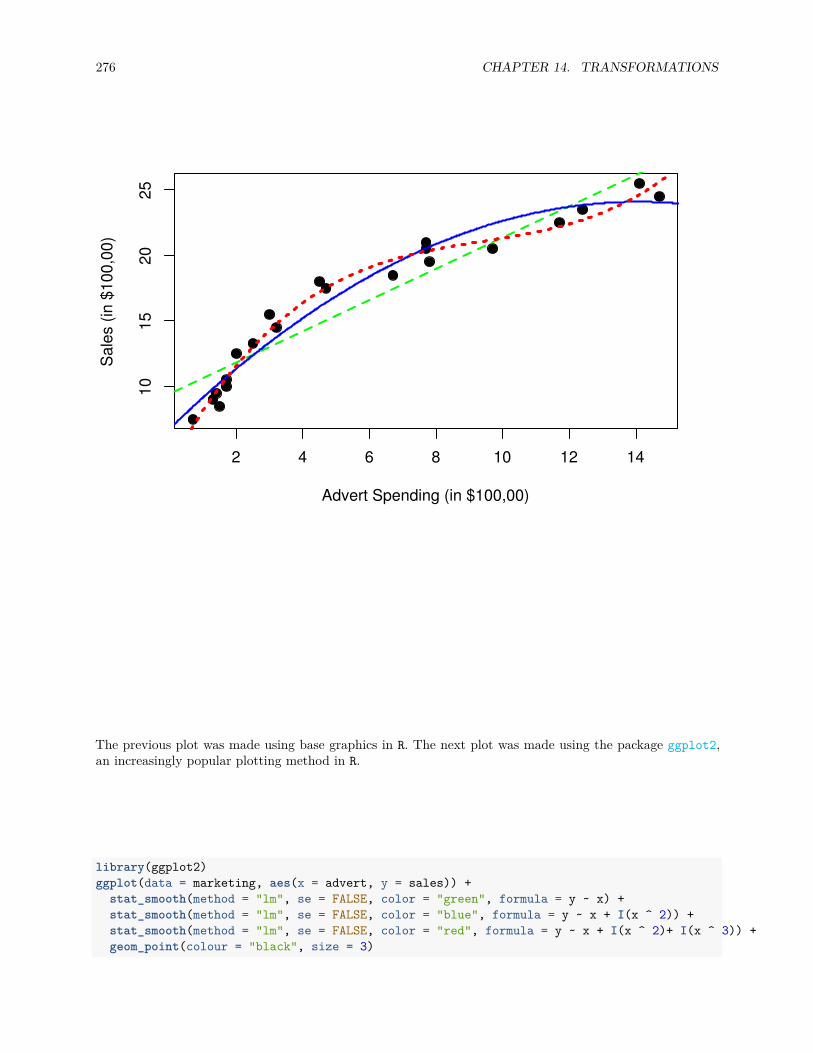
276 CHAPTER 14. TRANSFORMATIONS
2 4 6 8 10 12 14
1015
2025
Advert Spending (in $100,00)
Sal
es (i
n $1
00,0
0)
The previous plot was made using base graphics in R. The next plot was made using the package ggplot2,an increasingly popular plotting method in R.
library(ggplot2)ggplot(data = marketing, aes(x = advert, y = sales)) +
stat_smooth(method = "lm", se = FALSE, color = "green", formula = y ~ x) +stat_smooth(method = "lm", se = FALSE, color = "blue", formula = y ~ x + I(x ^ 2)) +stat_smooth(method = "lm", se = FALSE, color = "red", formula = y ~ x + I(x ^ 2)+ I(x ^ 3)) +geom_point(colour = "black", size = 3)
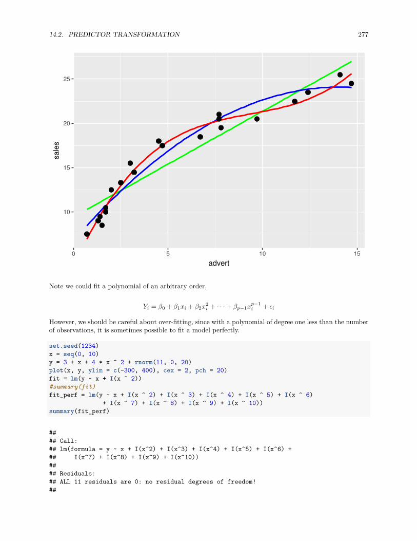
14.2. PREDICTOR TRANSFORMATION 277
10
15
20
25
0 5 10 15
advert
sale
s
Note we could fit a polynomial of an arbitrary order,
Yi = β0 + β1xi + β2x2i + · · · + βp−1xp−1
i + ϵi
However, we should be careful about over-fitting, since with a polynomial of degree one less than the numberof observations, it is sometimes possible to fit a model perfectly.
set.seed(1234)x = seq(0, 10)y = 3 + x + 4 * x ^ 2 + rnorm(11, 0, 20)plot(x, y, ylim = c(-300, 400), cex = 2, pch = 20)fit = lm(y ~ x + I(x ^ 2))#summary(fit)fit_perf = lm(y ~ x + I(x ^ 2) + I(x ^ 3) + I(x ^ 4) + I(x ^ 5) + I(x ^ 6)
+ I(x ^ 7) + I(x ^ 8) + I(x ^ 9) + I(x ^ 10))summary(fit_perf)
#### Call:## lm(formula = y ~ x + I(x^2) + I(x^3) + I(x^4) + I(x^5) + I(x^6) +## I(x^7) + I(x^8) + I(x^9) + I(x^10))#### Residuals:## ALL 11 residuals are 0: no residual degrees of freedom!##
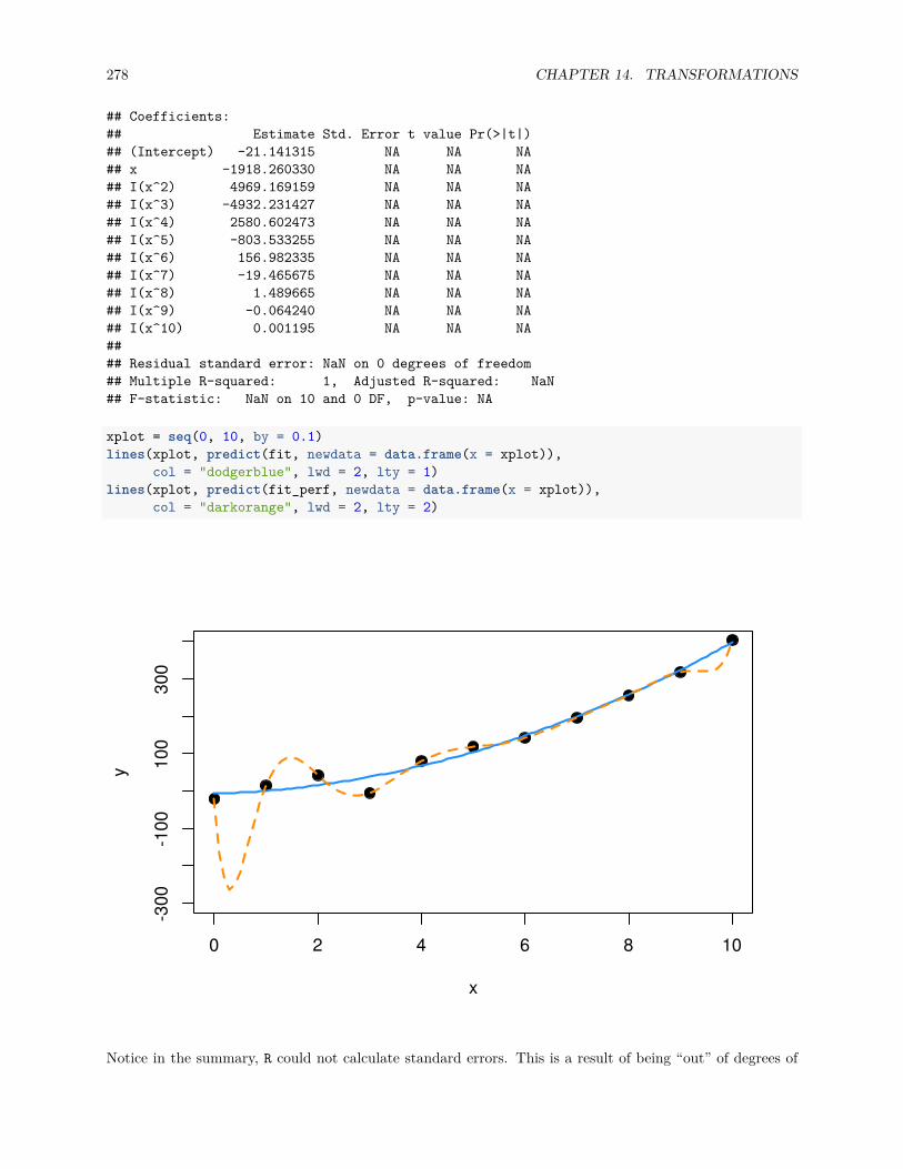
278 CHAPTER 14. TRANSFORMATIONS
## Coefficients:## Estimate Std. Error t value Pr(>|t|)## (Intercept) -21.141315 NA NA NA## x -1918.260330 NA NA NA## I(x^2) 4969.169159 NA NA NA## I(x^3) -4932.231427 NA NA NA## I(x^4) 2580.602473 NA NA NA## I(x^5) -803.533255 NA NA NA## I(x^6) 156.982335 NA NA NA## I(x^7) -19.465675 NA NA NA## I(x^8) 1.489665 NA NA NA## I(x^9) -0.064240 NA NA NA## I(x^10) 0.001195 NA NA NA#### Residual standard error: NaN on 0 degrees of freedom## Multiple R-squared: 1, Adjusted R-squared: NaN## F-statistic: NaN on 10 and 0 DF, p-value: NA
xplot = seq(0, 10, by = 0.1)lines(xplot, predict(fit, newdata = data.frame(x = xplot)),
col = "dodgerblue", lwd = 2, lty = 1)lines(xplot, predict(fit_perf, newdata = data.frame(x = xplot)),
col = "darkorange", lwd = 2, lty = 2)
0 2 4 6 8 10
-300
-100
100
300
x
y
Notice in the summary, R could not calculate standard errors. This is a result of being “out” of degrees of

14.2. PREDICTOR TRANSFORMATION 279
freedom. With 11 β parameters and 11 data points, we use up all the degrees of freedom before we canestimate σ.
In this example, the true relationship is quadratic, but the order 10 polynomial’s fit is “perfect”. Next chapterwe will focus on the trade-off between goodness of fit (minimizing errors) and complexity of model.
Suppose you work for an automobile manufacturer which makes a large luxury sedan. You would like toknow how the car performs from a fuel efficiency standpoint when it is driven at various speeds. Instead oftesting the car at every conceivable speed (which would be impossible) you create an experiment where thecar is driven at speeds of interest in increments of 5 miles per hour.
Our goal then, is to fit a model to this data in order to be able to predict fuel efficiency when driving atcertain speeds. The data from this example can be found in fuel_econ.csv.
econ = read.csv("data/fuel_econ.csv")
In this example, we will be frequently looking a the fitted versus residuals plot, so we should write a functionto make our life easier, but this is left as an exercise for homework.
We will also be adding fitted curves to scatterplots repeatedly, so smartly we will write a function to do so.
plot_econ_curve = function(model){plot(mpg ~ mph, data = econ, xlab = "Speed (Miles per Hour)",
ylab = "Fuel Efficiency (Miles per Gallon)", col = "dodgerblue",pch = 20, cex =2)
xplot = seq(10, 75, by = 0.1)lines(xplot, predict(model, newdata = data.frame(mph = xplot)),
col = "darkorange", lwd = 2, lty = 1)}
So now we first fit a simple linear regression to this data.
fit1 = lm(mpg ~ mph, data = econ)
par(mfrow = c(1, 2))plot_econ_curve(fit1)plot(fitted(fit1), resid(fit1), xlab = "Fitted", ylab = "Residuals",
col = "dodgerblue", pch = 20, cex =2)abline(h = 0, col = "darkorange", lwd = 2)
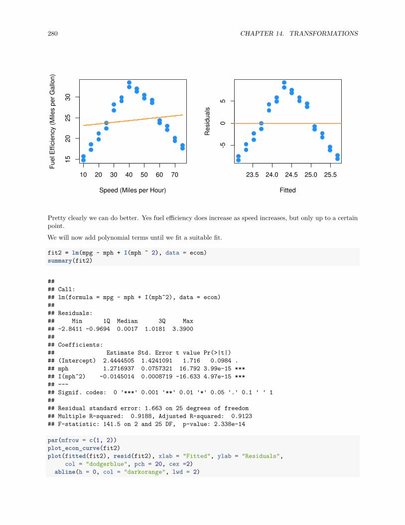
280 CHAPTER 14. TRANSFORMATIONS
10 20 30 40 50 60 70
1520
2530
Speed (Miles per Hour)
Fuel
Effi
cien
cy (M
iles
per G
allo
n)
23.5 24.0 24.5 25.0 25.5
-50
5
Fitted
Res
idua
ls
Pretty clearly we can do better. Yes fuel efficiency does increase as speed increases, but only up to a certainpoint.We will now add polynomial terms until we fit a suitable fit.
fit2 = lm(mpg ~ mph + I(mph ^ 2), data = econ)summary(fit2)
#### Call:## lm(formula = mpg ~ mph + I(mph^2), data = econ)#### Residuals:## Min 1Q Median 3Q Max## -2.8411 -0.9694 0.0017 1.0181 3.3900#### Coefficients:## Estimate Std. Error t value Pr(>|t|)## (Intercept) 2.4444505 1.4241091 1.716 0.0984 .## mph 1.2716937 0.0757321 16.792 3.99e-15 ***## I(mph^2) -0.0145014 0.0008719 -16.633 4.97e-15 ***## ---## Signif. codes: 0 '***' 0.001 '**' 0.01 '*' 0.05 '.' 0.1 ' ' 1#### Residual standard error: 1.663 on 25 degrees of freedom## Multiple R-squared: 0.9188, Adjusted R-squared: 0.9123## F-statistic: 141.5 on 2 and 25 DF, p-value: 2.338e-14
par(mfrow = c(1, 2))plot_econ_curve(fit2)plot(fitted(fit2), resid(fit2), xlab = "Fitted", ylab = "Residuals",
col = "dodgerblue", pch = 20, cex =2)abline(h = 0, col = "darkorange", lwd = 2)
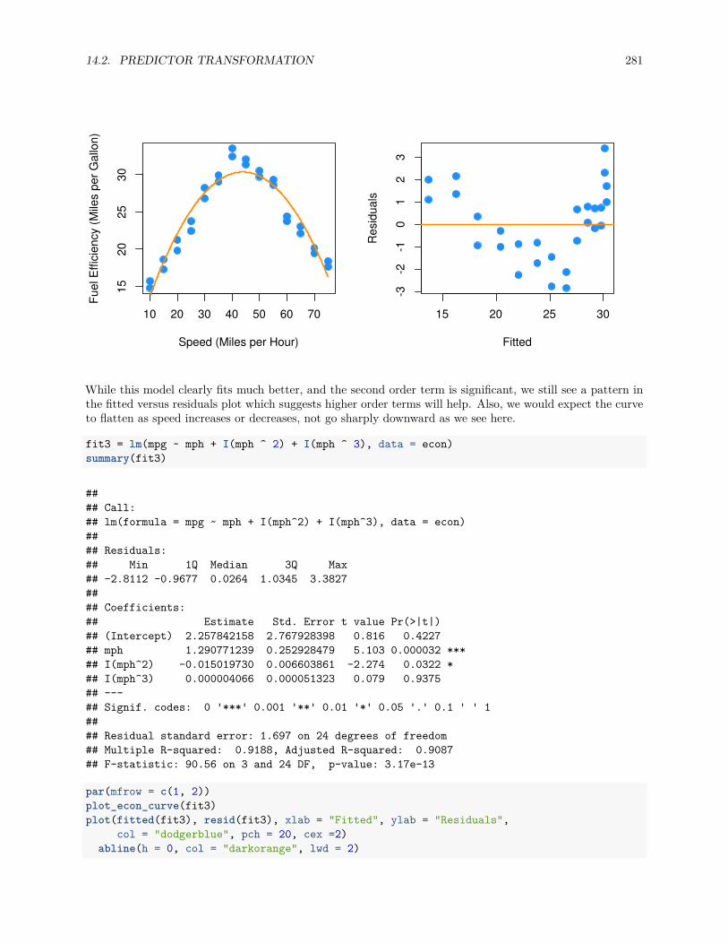
14.2. PREDICTOR TRANSFORMATION 281
10 20 30 40 50 60 70
1520
2530
Speed (Miles per Hour)
Fuel
Effi
cien
cy (M
iles
per G
allo
n)
15 20 25 30
-3-2
-10
12
3
Fitted
Res
idua
lsWhile this model clearly fits much better, and the second order term is significant, we still see a pattern inthe fitted versus residuals plot which suggests higher order terms will help. Also, we would expect the curveto flatten as speed increases or decreases, not go sharply downward as we see here.
fit3 = lm(mpg ~ mph + I(mph ^ 2) + I(mph ^ 3), data = econ)summary(fit3)
#### Call:## lm(formula = mpg ~ mph + I(mph^2) + I(mph^3), data = econ)#### Residuals:## Min 1Q Median 3Q Max## -2.8112 -0.9677 0.0264 1.0345 3.3827#### Coefficients:## Estimate Std. Error t value Pr(>|t|)## (Intercept) 2.257842158 2.767928398 0.816 0.4227## mph 1.290771239 0.252928479 5.103 0.000032 ***## I(mph^2) -0.015019730 0.006603861 -2.274 0.0322 *## I(mph^3) 0.000004066 0.000051323 0.079 0.9375## ---## Signif. codes: 0 '***' 0.001 '**' 0.01 '*' 0.05 '.' 0.1 ' ' 1#### Residual standard error: 1.697 on 24 degrees of freedom## Multiple R-squared: 0.9188, Adjusted R-squared: 0.9087## F-statistic: 90.56 on 3 and 24 DF, p-value: 3.17e-13
par(mfrow = c(1, 2))plot_econ_curve(fit3)plot(fitted(fit3), resid(fit3), xlab = "Fitted", ylab = "Residuals",
col = "dodgerblue", pch = 20, cex =2)abline(h = 0, col = "darkorange", lwd = 2)
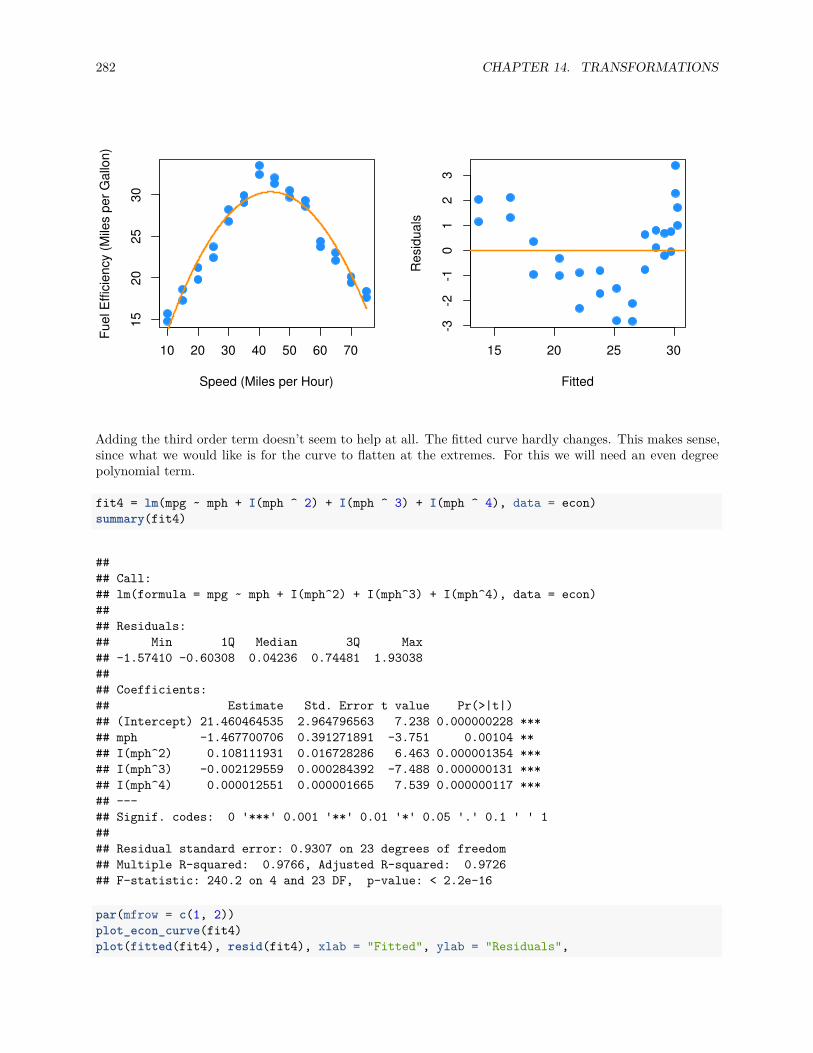
282 CHAPTER 14. TRANSFORMATIONS
10 20 30 40 50 60 70
1520
2530
Speed (Miles per Hour)
Fuel
Effi
cien
cy (M
iles
per G
allo
n)
15 20 25 30
-3-2
-10
12
3
Fitted
Res
idua
ls
Adding the third order term doesn’t seem to help at all. The fitted curve hardly changes. This makes sense,since what we would like is for the curve to flatten at the extremes. For this we will need an even degreepolynomial term.
fit4 = lm(mpg ~ mph + I(mph ^ 2) + I(mph ^ 3) + I(mph ^ 4), data = econ)summary(fit4)
#### Call:## lm(formula = mpg ~ mph + I(mph^2) + I(mph^3) + I(mph^4), data = econ)#### Residuals:## Min 1Q Median 3Q Max## -1.57410 -0.60308 0.04236 0.74481 1.93038#### Coefficients:## Estimate Std. Error t value Pr(>|t|)## (Intercept) 21.460464535 2.964796563 7.238 0.000000228 ***## mph -1.467700706 0.391271891 -3.751 0.00104 **## I(mph^2) 0.108111931 0.016728286 6.463 0.000001354 ***## I(mph^3) -0.002129559 0.000284392 -7.488 0.000000131 ***## I(mph^4) 0.000012551 0.000001665 7.539 0.000000117 ***## ---## Signif. codes: 0 '***' 0.001 '**' 0.01 '*' 0.05 '.' 0.1 ' ' 1#### Residual standard error: 0.9307 on 23 degrees of freedom## Multiple R-squared: 0.9766, Adjusted R-squared: 0.9726## F-statistic: 240.2 on 4 and 23 DF, p-value: < 2.2e-16
par(mfrow = c(1, 2))plot_econ_curve(fit4)plot(fitted(fit4), resid(fit4), xlab = "Fitted", ylab = "Residuals",
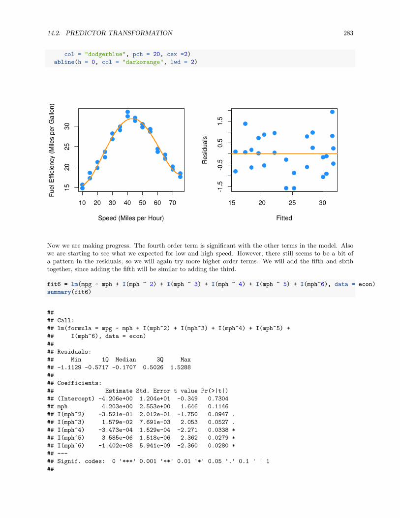
14.2. PREDICTOR TRANSFORMATION 283
col = "dodgerblue", pch = 20, cex =2)abline(h = 0, col = "darkorange", lwd = 2)
10 20 30 40 50 60 70
1520
2530
Speed (Miles per Hour)
Fuel
Effi
cien
cy (M
iles
per G
allo
n)
15 20 25 30
-1.5
-0.5
0.5
1.5
Fitted
Res
idua
ls
Now we are making progress. The fourth order term is significant with the other terms in the model. Alsowe are starting to see what we expected for low and high speed. However, there still seems to be a bit ofa pattern in the residuals, so we will again try more higher order terms. We will add the fifth and sixthtogether, since adding the fifth will be similar to adding the third.
fit6 = lm(mpg ~ mph + I(mph ^ 2) + I(mph ^ 3) + I(mph ^ 4) + I(mph ^ 5) + I(mph^6), data = econ)summary(fit6)
#### Call:## lm(formula = mpg ~ mph + I(mph^2) + I(mph^3) + I(mph^4) + I(mph^5) +## I(mph^6), data = econ)#### Residuals:## Min 1Q Median 3Q Max## -1.1129 -0.5717 -0.1707 0.5026 1.5288#### Coefficients:## Estimate Std. Error t value Pr(>|t|)## (Intercept) -4.206e+00 1.204e+01 -0.349 0.7304## mph 4.203e+00 2.553e+00 1.646 0.1146## I(mph^2) -3.521e-01 2.012e-01 -1.750 0.0947 .## I(mph^3) 1.579e-02 7.691e-03 2.053 0.0527 .## I(mph^4) -3.473e-04 1.529e-04 -2.271 0.0338 *## I(mph^5) 3.585e-06 1.518e-06 2.362 0.0279 *## I(mph^6) -1.402e-08 5.941e-09 -2.360 0.0280 *## ---## Signif. codes: 0 '***' 0.001 '**' 0.01 '*' 0.05 '.' 0.1 ' ' 1##
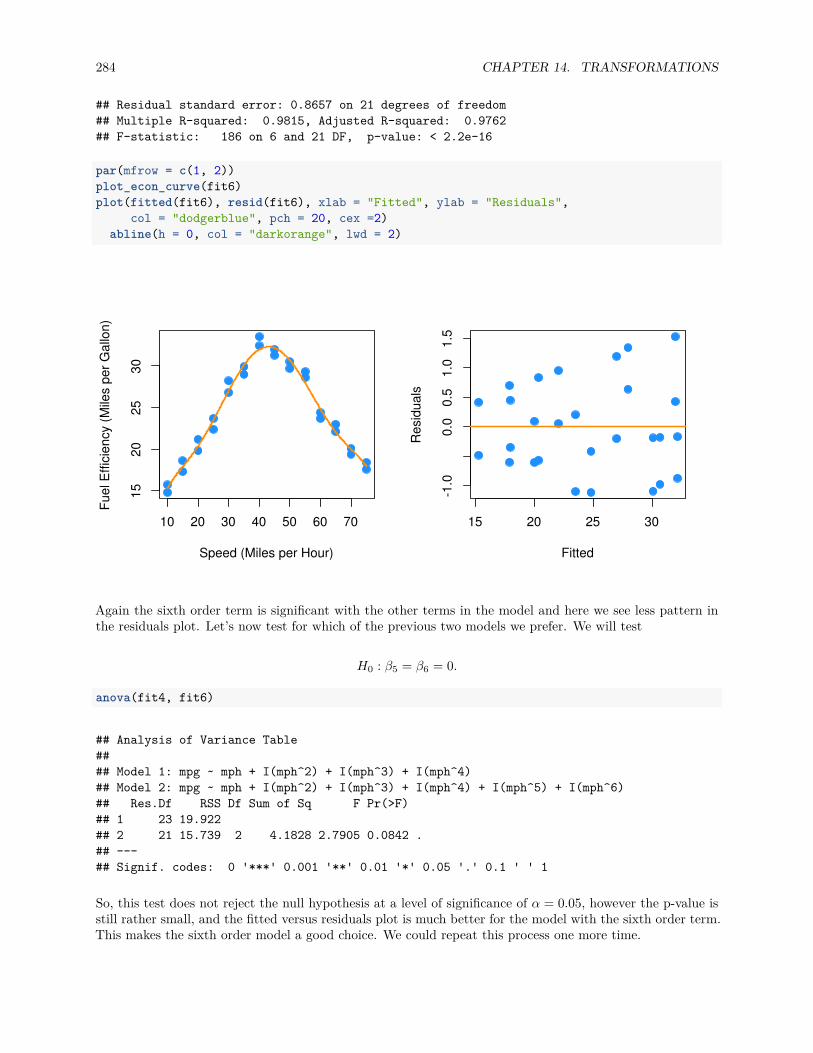
284 CHAPTER 14. TRANSFORMATIONS
## Residual standard error: 0.8657 on 21 degrees of freedom## Multiple R-squared: 0.9815, Adjusted R-squared: 0.9762## F-statistic: 186 on 6 and 21 DF, p-value: < 2.2e-16
par(mfrow = c(1, 2))plot_econ_curve(fit6)plot(fitted(fit6), resid(fit6), xlab = "Fitted", ylab = "Residuals",
col = "dodgerblue", pch = 20, cex =2)abline(h = 0, col = "darkorange", lwd = 2)
10 20 30 40 50 60 70
1520
2530
Speed (Miles per Hour)
Fuel
Effi
cien
cy (M
iles
per G
allo
n)
15 20 25 30
-1.0
0.0
0.5
1.0
1.5
Fitted
Res
idua
ls
Again the sixth order term is significant with the other terms in the model and here we see less pattern inthe residuals plot. Let’s now test for which of the previous two models we prefer. We will test
H0 : β5 = β6 = 0.
anova(fit4, fit6)
## Analysis of Variance Table#### Model 1: mpg ~ mph + I(mph^2) + I(mph^3) + I(mph^4)## Model 2: mpg ~ mph + I(mph^2) + I(mph^3) + I(mph^4) + I(mph^5) + I(mph^6)## Res.Df RSS Df Sum of Sq F Pr(>F)## 1 23 19.922## 2 21 15.739 2 4.1828 2.7905 0.0842 .## ---## Signif. codes: 0 '***' 0.001 '**' 0.01 '*' 0.05 '.' 0.1 ' ' 1
So, this test does not reject the null hypothesis at a level of significance of α = 0.05, however the p-value isstill rather small, and the fitted versus residuals plot is much better for the model with the sixth order term.This makes the sixth order model a good choice. We could repeat this process one more time.

14.2. PREDICTOR TRANSFORMATION 285
fit8 = lm(mpg ~ mph + I(mph ^ 2) + I(mph ^ 3) + I(mph ^ 4) + I(mph ^ 5)+ I(mph ^ 6) + I(mph ^ 7) + I(mph ^ 8), data = econ)
summary(fit8)
#### Call:## lm(formula = mpg ~ mph + I(mph^2) + I(mph^3) + I(mph^4) + I(mph^5) +## I(mph^6) + I(mph^7) + I(mph^8), data = econ)#### Residuals:## Min 1Q Median 3Q Max## -1.21938 -0.50464 -0.09105 0.49029 1.45440#### Coefficients:## Estimate Std. Error t value Pr(>|t|)## (Intercept) -1.202e+01 7.045e+01 -0.171 0.866## mph 6.021e+00 2.014e+01 0.299 0.768## I(mph^2) -5.037e-01 2.313e+00 -0.218 0.830## I(mph^3) 2.121e-02 1.408e-01 0.151 0.882## I(mph^4) -4.008e-04 5.017e-03 -0.080 0.937## I(mph^5) 1.789e-06 1.080e-04 0.017 0.987## I(mph^6) 4.486e-08 1.381e-06 0.032 0.974## I(mph^7) -6.456e-10 9.649e-09 -0.067 0.947## I(mph^8) 2.530e-12 2.835e-11 0.089 0.930#### Residual standard error: 0.9034 on 19 degrees of freedom## Multiple R-squared: 0.9818, Adjusted R-squared: 0.9741## F-statistic: 128.1 on 8 and 19 DF, p-value: 7.074e-15
par(mfrow = c(1, 2))plot_econ_curve(fit8)plot(fitted(fit8), resid(fit8), xlab = "Fitted", ylab = "Residuals",
col = "dodgerblue", pch = 20, cex =2)abline(h = 0, col = "darkorange", lwd = 2)
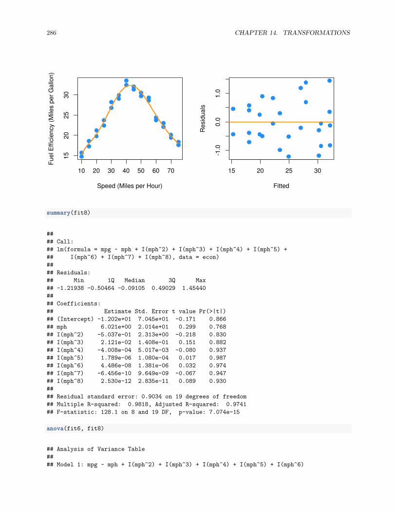
286 CHAPTER 14. TRANSFORMATIONS
10 20 30 40 50 60 70
1520
2530
Speed (Miles per Hour)
Fuel
Effi
cien
cy (M
iles
per G
allo
n)
15 20 25 30
-1.0
0.0
1.0
Fitted
Res
idua
ls
summary(fit8)
#### Call:## lm(formula = mpg ~ mph + I(mph^2) + I(mph^3) + I(mph^4) + I(mph^5) +## I(mph^6) + I(mph^7) + I(mph^8), data = econ)#### Residuals:## Min 1Q Median 3Q Max## -1.21938 -0.50464 -0.09105 0.49029 1.45440#### Coefficients:## Estimate Std. Error t value Pr(>|t|)## (Intercept) -1.202e+01 7.045e+01 -0.171 0.866## mph 6.021e+00 2.014e+01 0.299 0.768## I(mph^2) -5.037e-01 2.313e+00 -0.218 0.830## I(mph^3) 2.121e-02 1.408e-01 0.151 0.882## I(mph^4) -4.008e-04 5.017e-03 -0.080 0.937## I(mph^5) 1.789e-06 1.080e-04 0.017 0.987## I(mph^6) 4.486e-08 1.381e-06 0.032 0.974## I(mph^7) -6.456e-10 9.649e-09 -0.067 0.947## I(mph^8) 2.530e-12 2.835e-11 0.089 0.930#### Residual standard error: 0.9034 on 19 degrees of freedom## Multiple R-squared: 0.9818, Adjusted R-squared: 0.9741## F-statistic: 128.1 on 8 and 19 DF, p-value: 7.074e-15
anova(fit6, fit8)
## Analysis of Variance Table#### Model 1: mpg ~ mph + I(mph^2) + I(mph^3) + I(mph^4) + I(mph^5) + I(mph^6)

14.2. PREDICTOR TRANSFORMATION 287
## Model 2: mpg ~ mph + I(mph^2) + I(mph^3) + I(mph^4) + I(mph^5) + I(mph^6) +## I(mph^7) + I(mph^8)## Res.Df RSS Df Sum of Sq F Pr(>F)## 1 21 15.739## 2 19 15.506 2 0.2324 0.1424 0.8682
Here we would clearly stick with fit6. The eighth order term is not significant with the other terms in themodel and the F-test does not reject.
As an aside, be aware that there is a quicker way to specify a model with many higher order terms.
fit6_alt = lm(mpg ~ poly(mph, 6), data = econ)all.equal(fitted(fit6), fitted(fit6_alt))
## [1] TRUE
We first verify that this method produces the same fitted values. However, the estimated coefficients aredifferent.
coef(fit6)
## (Intercept) mph I(mph^2) I(mph^3)## -4.20622377616269 4.20338221905924 -0.35214523989512 0.01579340288449## I(mph^4) I(mph^5) I(mph^6)## -0.00034726647879 0.00000358520124 -0.00000001401995
coef(fit6_alt)
## (Intercept) poly(mph, 6)1 poly(mph, 6)2 poly(mph, 6)3 poly(mph, 6)4## 24.40714286 4.16769628 -27.66685755 0.13446747 7.01671480## poly(mph, 6)5 poly(mph, 6)6## 0.09288754 -2.04307796
This is because poly() uses orthogonal polynimials, which solves an issue we will discuss in the next chapter.
summary(fit6)
#### Call:## lm(formula = mpg ~ mph + I(mph^2) + I(mph^3) + I(mph^4) + I(mph^5) +## I(mph^6), data = econ)#### Residuals:## Min 1Q Median 3Q Max## -1.1129 -0.5717 -0.1707 0.5026 1.5288#### Coefficients:## Estimate Std. Error t value Pr(>|t|)## (Intercept) -4.206e+00 1.204e+01 -0.349 0.7304## mph 4.203e+00 2.553e+00 1.646 0.1146## I(mph^2) -3.521e-01 2.012e-01 -1.750 0.0947 .
288 CHAPTER 14. TRANSFORMATIONS
## I(mph^3) 1.579e-02 7.691e-03 2.053 0.0527 .## I(mph^4) -3.473e-04 1.529e-04 -2.271 0.0338 *## I(mph^5) 3.585e-06 1.518e-06 2.362 0.0279 *## I(mph^6) -1.402e-08 5.941e-09 -2.360 0.0280 *## ---## Signif. codes: 0 '***' 0.001 '**' 0.01 '*' 0.05 '.' 0.1 ' ' 1#### Residual standard error: 0.8657 on 21 degrees of freedom## Multiple R-squared: 0.9815, Adjusted R-squared: 0.9762## F-statistic: 186 on 6 and 21 DF, p-value: < 2.2e-16
summary(fit6_alt)
#### Call:## lm(formula = mpg ~ poly(mph, 6), data = econ)#### Residuals:## Min 1Q Median 3Q Max## -1.1129 -0.5717 -0.1707 0.5026 1.5288#### Coefficients:## Estimate Std. Error t value Pr(>|t|)## (Intercept) 24.40714 0.16360 149.184 < 2e-16 ***## poly(mph, 6)1 4.16770 0.86571 4.814 0.0000930613 ***## poly(mph, 6)2 -27.66686 0.86571 -31.958 < 2e-16 ***## poly(mph, 6)3 0.13447 0.86571 0.155 0.878## poly(mph, 6)4 7.01671 0.86571 8.105 0.0000000668 ***## poly(mph, 6)5 0.09289 0.86571 0.107 0.916## poly(mph, 6)6 -2.04308 0.86571 -2.360 0.028 *## ---## Signif. codes: 0 '***' 0.001 '**' 0.01 '*' 0.05 '.' 0.1 ' ' 1#### Residual standard error: 0.8657 on 21 degrees of freedom## Multiple R-squared: 0.9815, Adjusted R-squared: 0.9762## F-statistic: 186 on 6 and 21 DF, p-value: < 2.2e-16
Notice though that the p-value for testing the degree 6 term is the same. Because of this, for the most partwe can use these interchangeably.To use poly() to obtain the same results as using I() repeatedly, we would need to set raw = TRUE.
fit6_alt2 = lm(mpg ~ poly(mph, 6, raw = TRUE), data = econ)coef(fit6_alt2)
## (Intercept) poly(mph, 6, raw = TRUE)1 poly(mph, 6, raw = TRUE)2## -4.20622377616269 4.20338221905924 -0.35214523989512## poly(mph, 6, raw = TRUE)3 poly(mph, 6, raw = TRUE)4 poly(mph, 6, raw = TRUE)5## 0.01579340288449 -0.00034726647879 0.00000358520124## poly(mph, 6, raw = TRUE)6## -0.00000001401995
We’ve now seen how to transform predictor and response variables. In this chapter we have mostly focusedon using this in the context of fixing SLR models. However, these concepts can easily be used together with
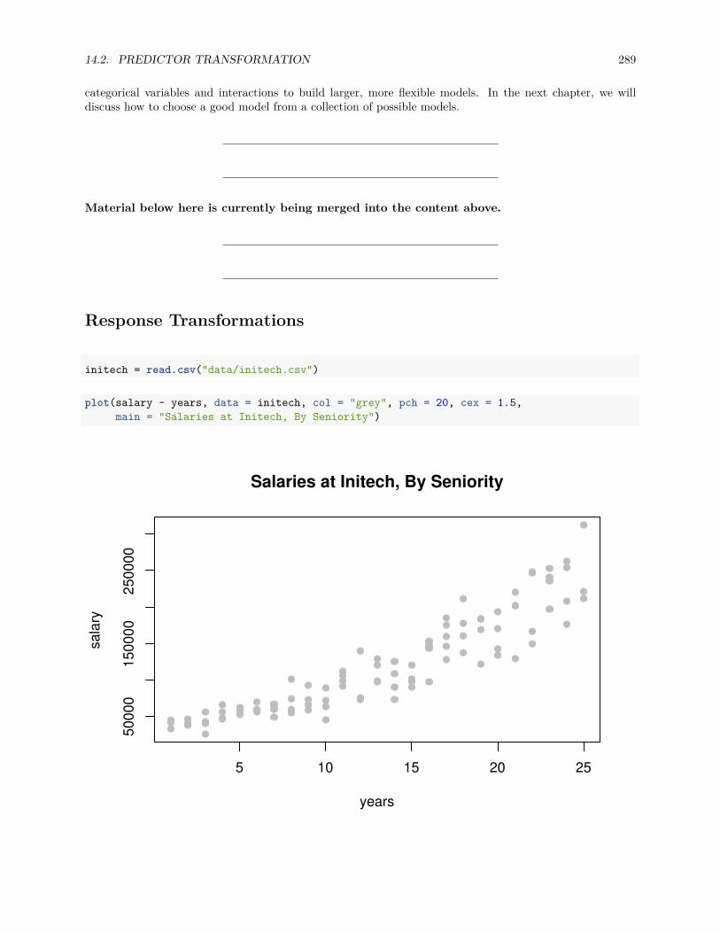
14.2. PREDICTOR TRANSFORMATION 289
categorical variables and interactions to build larger, more flexible models. In the next chapter, we willdiscuss how to choose a good model from a collection of possible models.
Material below here is currently being merged into the content above.
Response Transformations
initech = read.csv("data/initech.csv")
plot(salary ~ years, data = initech, col = "grey", pch = 20, cex = 1.5,main = "Salaries at Initech, By Seniority")
5 10 15 20 25
5000
015
0000
2500
00
Salaries at Initech, By Seniority
years
sala
ry
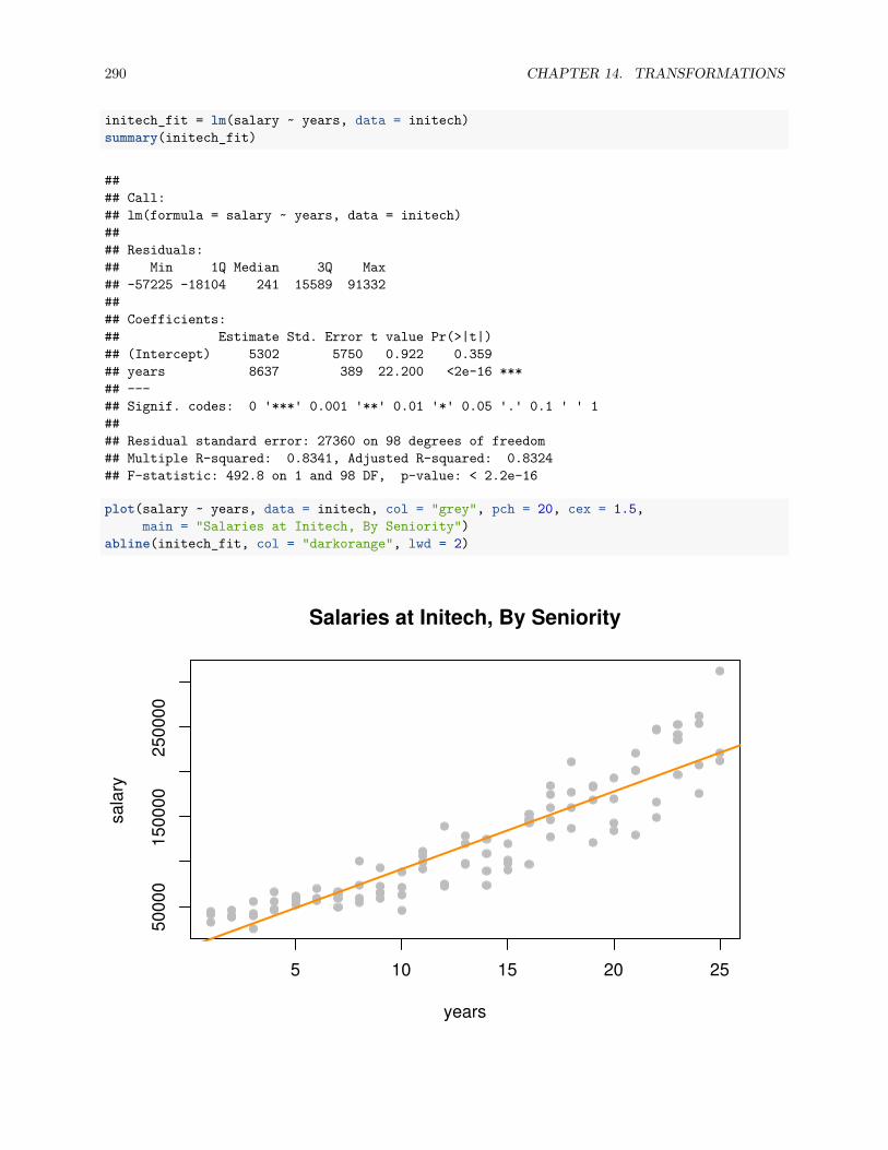
290 CHAPTER 14. TRANSFORMATIONS
initech_fit = lm(salary ~ years, data = initech)summary(initech_fit)
#### Call:## lm(formula = salary ~ years, data = initech)#### Residuals:## Min 1Q Median 3Q Max## -57225 -18104 241 15589 91332#### Coefficients:## Estimate Std. Error t value Pr(>|t|)## (Intercept) 5302 5750 0.922 0.359## years 8637 389 22.200 <2e-16 ***## ---## Signif. codes: 0 '***' 0.001 '**' 0.01 '*' 0.05 '.' 0.1 ' ' 1#### Residual standard error: 27360 on 98 degrees of freedom## Multiple R-squared: 0.8341, Adjusted R-squared: 0.8324## F-statistic: 492.8 on 1 and 98 DF, p-value: < 2.2e-16
plot(salary ~ years, data = initech, col = "grey", pch = 20, cex = 1.5,main = "Salaries at Initech, By Seniority")
abline(initech_fit, col = "darkorange", lwd = 2)
5 10 15 20 25
5000
015
0000
2500
00
Salaries at Initech, By Seniority
years
sala
ry
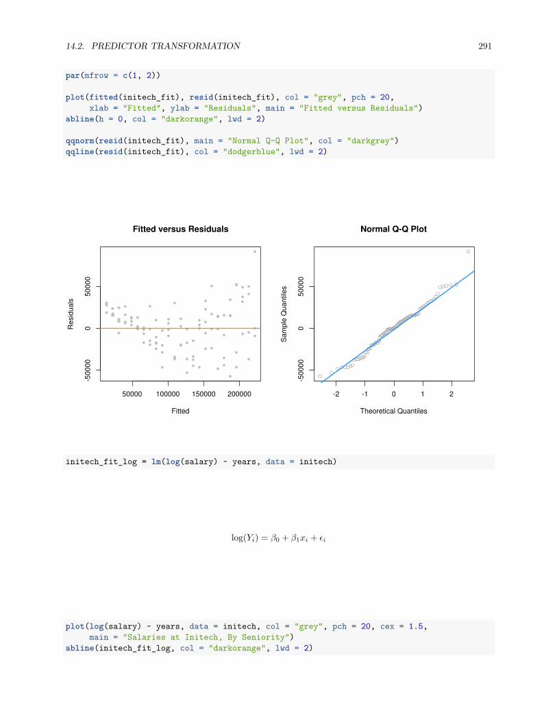
14.2. PREDICTOR TRANSFORMATION 291
par(mfrow = c(1, 2))
plot(fitted(initech_fit), resid(initech_fit), col = "grey", pch = 20,xlab = "Fitted", ylab = "Residuals", main = "Fitted versus Residuals")
abline(h = 0, col = "darkorange", lwd = 2)
qqnorm(resid(initech_fit), main = "Normal Q-Q Plot", col = "darkgrey")qqline(resid(initech_fit), col = "dodgerblue", lwd = 2)
50000 100000 150000 200000
-500
000
5000
0
Fitted versus Residuals
Fitted
Res
idua
ls
-2 -1 0 1 2
-500
000
5000
0
Normal Q-Q Plot
Theoretical Quantiles
Sam
ple
Qua
ntile
s
initech_fit_log = lm(log(salary) ~ years, data = initech)
log(Yi) = β0 + β1xi + ϵi
plot(log(salary) ~ years, data = initech, col = "grey", pch = 20, cex = 1.5,main = "Salaries at Initech, By Seniority")
abline(initech_fit_log, col = "darkorange", lwd = 2)
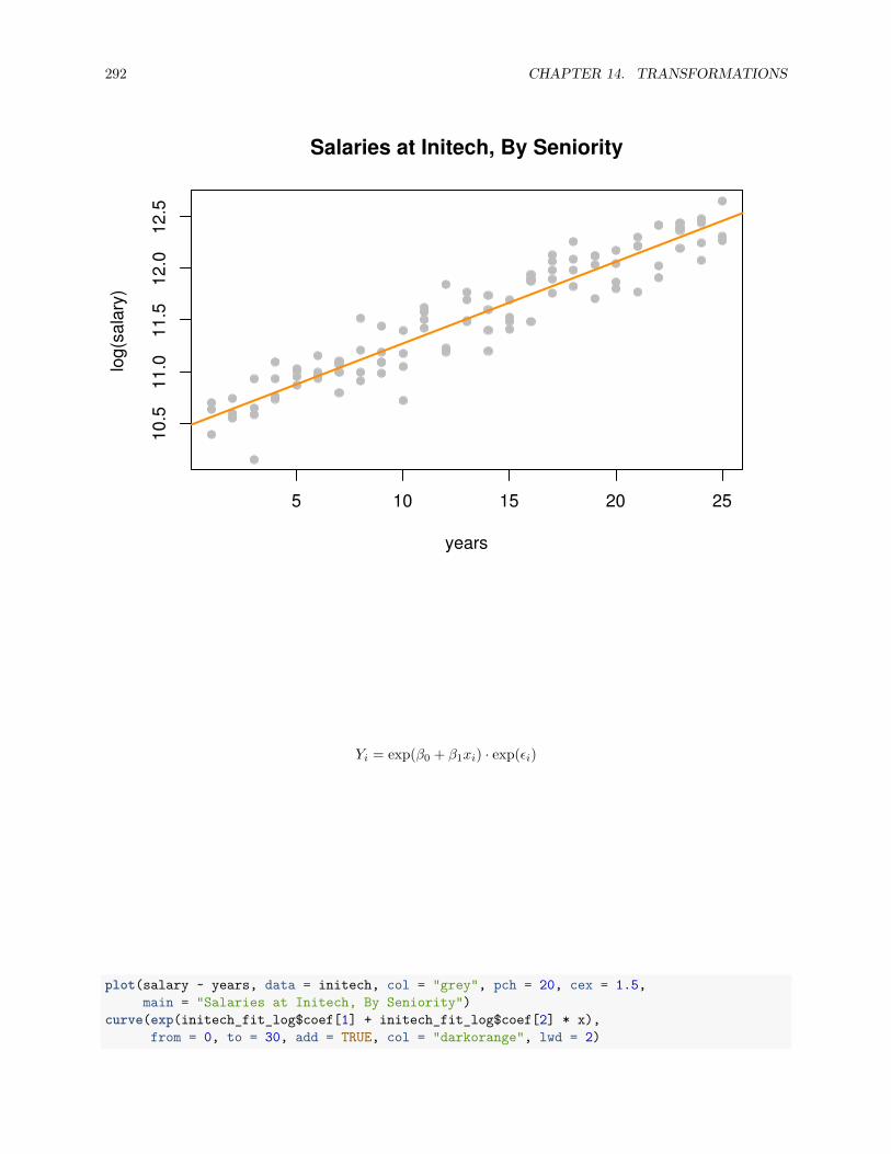
292 CHAPTER 14. TRANSFORMATIONS
5 10 15 20 25
10.5
11.0
11.5
12.0
12.5
Salaries at Initech, By Seniority
years
log(
sala
ry)
Yi = exp(β0 + β1xi) · exp(ϵi)
plot(salary ~ years, data = initech, col = "grey", pch = 20, cex = 1.5,main = "Salaries at Initech, By Seniority")
curve(exp(initech_fit_log$coef[1] + initech_fit_log$coef[2] * x),from = 0, to = 30, add = TRUE, col = "darkorange", lwd = 2)
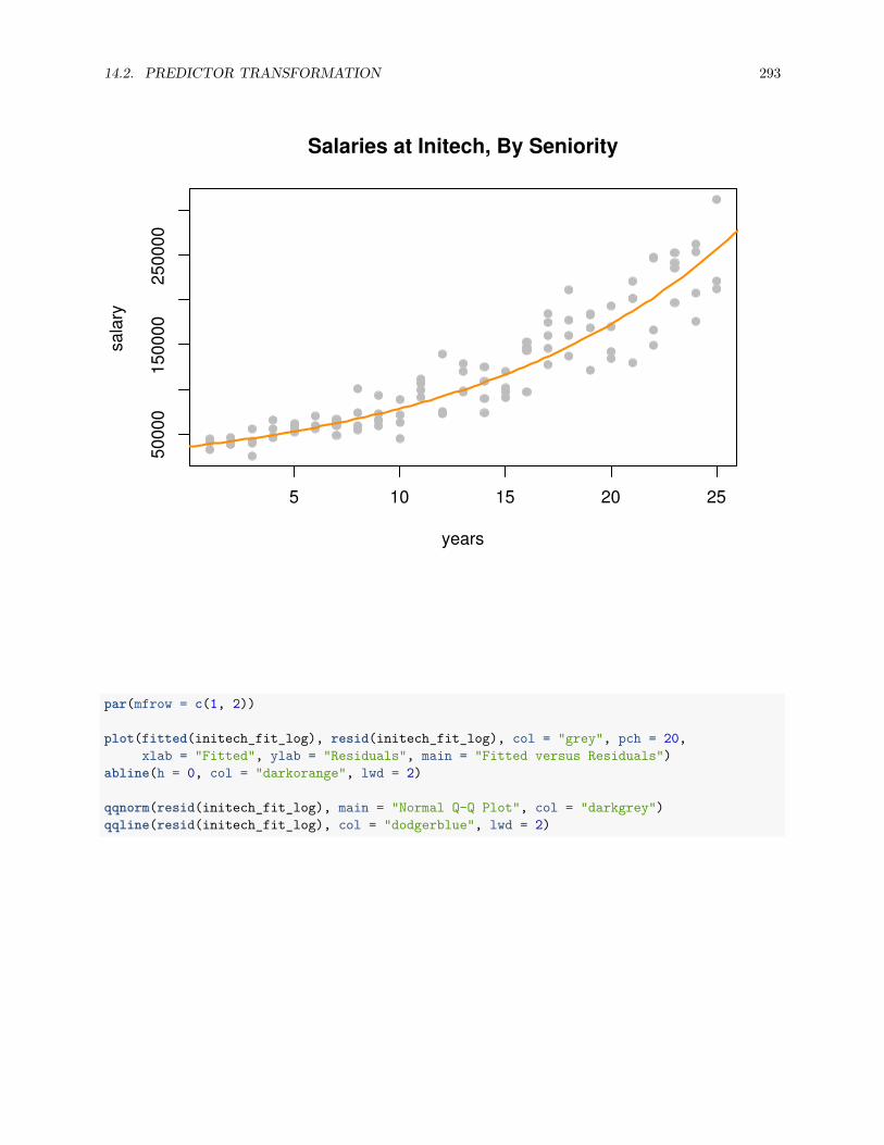
14.2. PREDICTOR TRANSFORMATION 293
5 10 15 20 25
5000
015
0000
2500
00Salaries at Initech, By Seniority
years
sala
ry
par(mfrow = c(1, 2))
plot(fitted(initech_fit_log), resid(initech_fit_log), col = "grey", pch = 20,xlab = "Fitted", ylab = "Residuals", main = "Fitted versus Residuals")
abline(h = 0, col = "darkorange", lwd = 2)
qqnorm(resid(initech_fit_log), main = "Normal Q-Q Plot", col = "darkgrey")qqline(resid(initech_fit_log), col = "dodgerblue", lwd = 2)
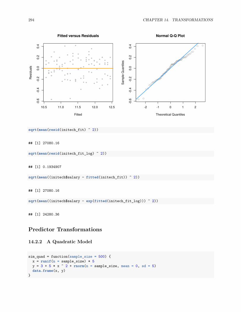
294 CHAPTER 14. TRANSFORMATIONS
10.5 11.0 11.5 12.0 12.5
-0.6
-0.4
-0.2
0.0
0.2
0.4
Fitted versus Residuals
Fitted
Res
idua
ls
-2 -1 0 1 2
-0.6
-0.4
-0.2
0.0
0.2
0.4
Normal Q-Q Plot
Theoretical Quantiles
Sam
ple
Qua
ntile
s
sqrt(mean(resid(initech_fit) ^ 2))
## [1] 27080.16
sqrt(mean(resid(initech_fit_log) ^ 2))
## [1] 0.1934907
sqrt(mean((initech$salary - fitted(initech_fit)) ^ 2))
## [1] 27080.16
sqrt(mean((initech$salary - exp(fitted(initech_fit_log))) ^ 2))
## [1] 24280.36
Predictor Transformations
14.2.2 A Quadratic Model
sim_quad = function(sample_size = 500) {x = runif(n = sample_size) * 5y = 3 + 5 * x ^ 2 + rnorm(n = sample_size, mean = 0, sd = 5)data.frame(x, y)
}

14.2. PREDICTOR TRANSFORMATION 295
set.seed(314)quad_data = sim_quad(sample_size = 200)
lin_fit = lm(y ~ x, data = quad_data)summary(lin_fit)
#### Call:## lm(formula = y ~ x, data = quad_data)#### Residuals:## Min 1Q Median 3Q Max## -20.363 -7.550 -3.416 8.472 26.181#### Coefficients:## Estimate Std. Error t value Pr(>|t|)## (Intercept) -18.3271 1.5494 -11.83 <2e-16 ***## x 24.8716 0.5343 46.55 <2e-16 ***## ---## Signif. codes: 0 '***' 0.001 '**' 0.01 '*' 0.05 '.' 0.1 ' ' 1#### Residual standard error: 10.79 on 198 degrees of freedom## Multiple R-squared: 0.9163, Adjusted R-squared: 0.9158## F-statistic: 2167 on 1 and 198 DF, p-value: < 2.2e-16
plot(y ~ x, data = quad_data, col = "grey", pch = 20, cex = 1.5,main = "Simulated Quadratic Data")
abline(lin_fit, col = "darkorange", lwd = 2)
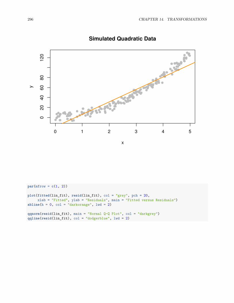
296 CHAPTER 14. TRANSFORMATIONS
0 1 2 3 4 5
020
4060
8012
0Simulated Quadratic Data
x
y
par(mfrow = c(1, 2))
plot(fitted(lin_fit), resid(lin_fit), col = "grey", pch = 20,xlab = "Fitted", ylab = "Residuals", main = "Fitted versus Residuals")
abline(h = 0, col = "darkorange", lwd = 2)
qqnorm(resid(lin_fit), main = "Normal Q-Q Plot", col = "darkgrey")qqline(resid(lin_fit), col = "dodgerblue", lwd = 2)
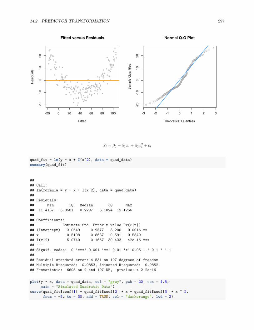
14.2. PREDICTOR TRANSFORMATION 297
-20 0 20 40 60 80 100
-20
-10
010
20Fitted versus Residuals
Fitted
Res
idua
ls
-3 -2 -1 0 1 2 3
-20
-10
010
20
Normal Q-Q Plot
Theoretical Quantiles
Sam
ple
Qua
ntile
s
Yi = β0 + β1xi + β2x2i + ϵi
quad_fit = lm(y ~ x + I(x^2), data = quad_data)summary(quad_fit)
#### Call:## lm(formula = y ~ x + I(x^2), data = quad_data)#### Residuals:## Min 1Q Median 3Q Max## -11.4167 -3.0581 0.2297 3.1024 12.1256#### Coefficients:## Estimate Std. Error t value Pr(>|t|)## (Intercept) 3.0649 0.9577 3.200 0.0016 **## x -0.5108 0.8637 -0.591 0.5549## I(x^2) 5.0740 0.1667 30.433 <2e-16 ***## ---## Signif. codes: 0 '***' 0.001 '**' 0.01 '*' 0.05 '.' 0.1 ' ' 1#### Residual standard error: 4.531 on 197 degrees of freedom## Multiple R-squared: 0.9853, Adjusted R-squared: 0.9852## F-statistic: 6608 on 2 and 197 DF, p-value: < 2.2e-16
plot(y ~ x, data = quad_data, col = "grey", pch = 20, cex = 1.5,main = "Simulated Quadratic Data")
curve(quad_fit$coef[1] + quad_fit$coef[2] * x + quad_fit$coef[3] * x ^ 2,from = -5, to = 30, add = TRUE, col = "darkorange", lwd = 2)
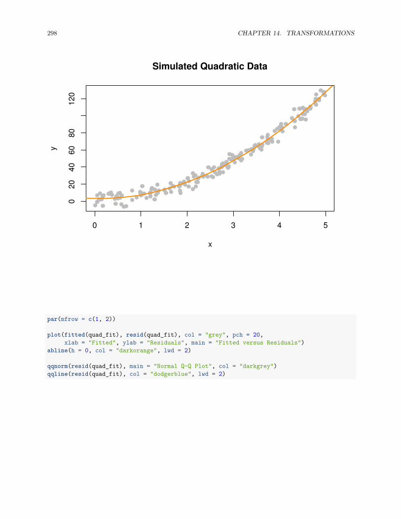
298 CHAPTER 14. TRANSFORMATIONS
0 1 2 3 4 5
020
4060
8012
0Simulated Quadratic Data
x
y
par(mfrow = c(1, 2))
plot(fitted(quad_fit), resid(quad_fit), col = "grey", pch = 20,xlab = "Fitted", ylab = "Residuals", main = "Fitted versus Residuals")
abline(h = 0, col = "darkorange", lwd = 2)
qqnorm(resid(quad_fit), main = "Normal Q-Q Plot", col = "darkgrey")qqline(resid(quad_fit), col = "dodgerblue", lwd = 2)
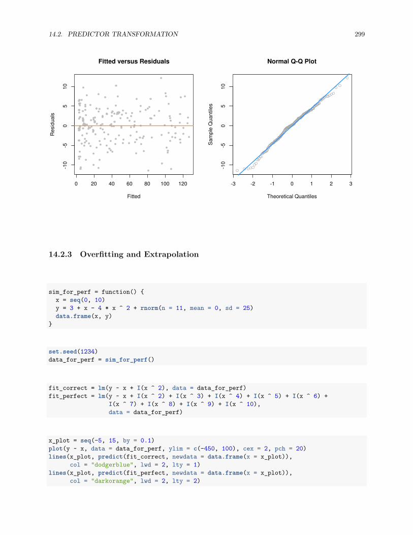
14.2. PREDICTOR TRANSFORMATION 299
0 20 40 60 80 100 120
-10
-50
510
Fitted versus Residuals
Fitted
Res
idua
ls
-3 -2 -1 0 1 2 3
-10
-50
510
Normal Q-Q Plot
Theoretical Quantiles
Sam
ple
Qua
ntile
s
14.2.3 Overfitting and Extrapolation
sim_for_perf = function() {x = seq(0, 10)y = 3 + x - 4 * x ^ 2 + rnorm(n = 11, mean = 0, sd = 25)data.frame(x, y)
}
set.seed(1234)data_for_perf = sim_for_perf()
fit_correct = lm(y ~ x + I(x ^ 2), data = data_for_perf)fit_perfect = lm(y ~ x + I(x ^ 2) + I(x ^ 3) + I(x ^ 4) + I(x ^ 5) + I(x ^ 6) +
I(x ^ 7) + I(x ^ 8) + I(x ^ 9) + I(x ^ 10),data = data_for_perf)
x_plot = seq(-5, 15, by = 0.1)plot(y ~ x, data = data_for_perf, ylim = c(-450, 100), cex = 2, pch = 20)lines(x_plot, predict(fit_correct, newdata = data.frame(x = x_plot)),
col = "dodgerblue", lwd = 2, lty = 1)lines(x_plot, predict(fit_perfect, newdata = data.frame(x = x_plot)),
col = "darkorange", lwd = 2, lty = 2)
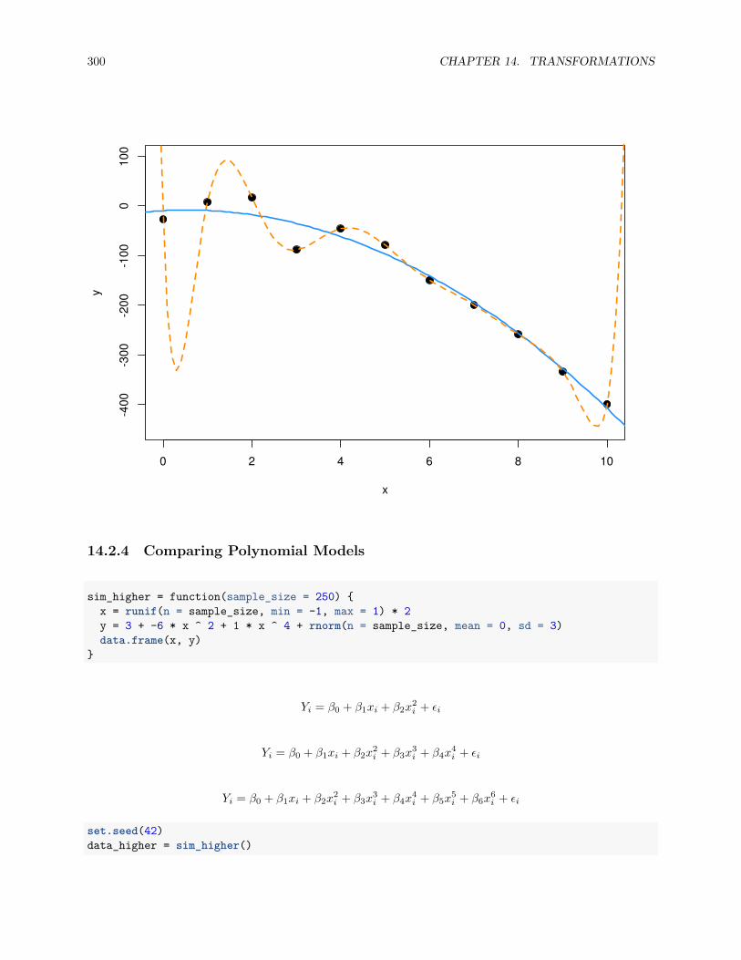
300 CHAPTER 14. TRANSFORMATIONS
0 2 4 6 8 10
-400
-300
-200
-100
010
0
x
y
14.2.4 Comparing Polynomial Models
sim_higher = function(sample_size = 250) {x = runif(n = sample_size, min = -1, max = 1) * 2y = 3 + -6 * x ^ 2 + 1 * x ^ 4 + rnorm(n = sample_size, mean = 0, sd = 3)data.frame(x, y)
}
Yi = β0 + β1xi + β2x2i + ϵi
Yi = β0 + β1xi + β2x2i + β3x3
i + β4x4i + ϵi
Yi = β0 + β1xi + β2x2i + β3x3
i + β4x4i + β5x5
i + β6x6i + ϵi
set.seed(42)data_higher = sim_higher()

14.2. PREDICTOR TRANSFORMATION 301
plot(y ~ x, data = data_higher, col = "grey", pch = 20, cex = 1.5,main = "Simulated Quartic Data")
-2 -1 0 1 2
-10
-50
510
Simulated Quartic Data
x
y
fit_2 = lm(y ~ poly(x, 2), data = data_higher)fit_4 = lm(y ~ poly(x, 4), data = data_higher)
plot(y ~ x, data = data_higher, col = "grey", pch = 20, cex = 1.5,main = "Simulated Quartic Data")
x_plot = seq(-5, 5, by = 0.05)lines(x_plot, predict(fit_2, newdata = data.frame(x = x_plot)),
col = "dodgerblue", lwd = 2, lty = 1)lines(x_plot, predict(fit_4, newdata = data.frame(x = x_plot)),
col = "darkorange", lwd = 2, lty = 2)
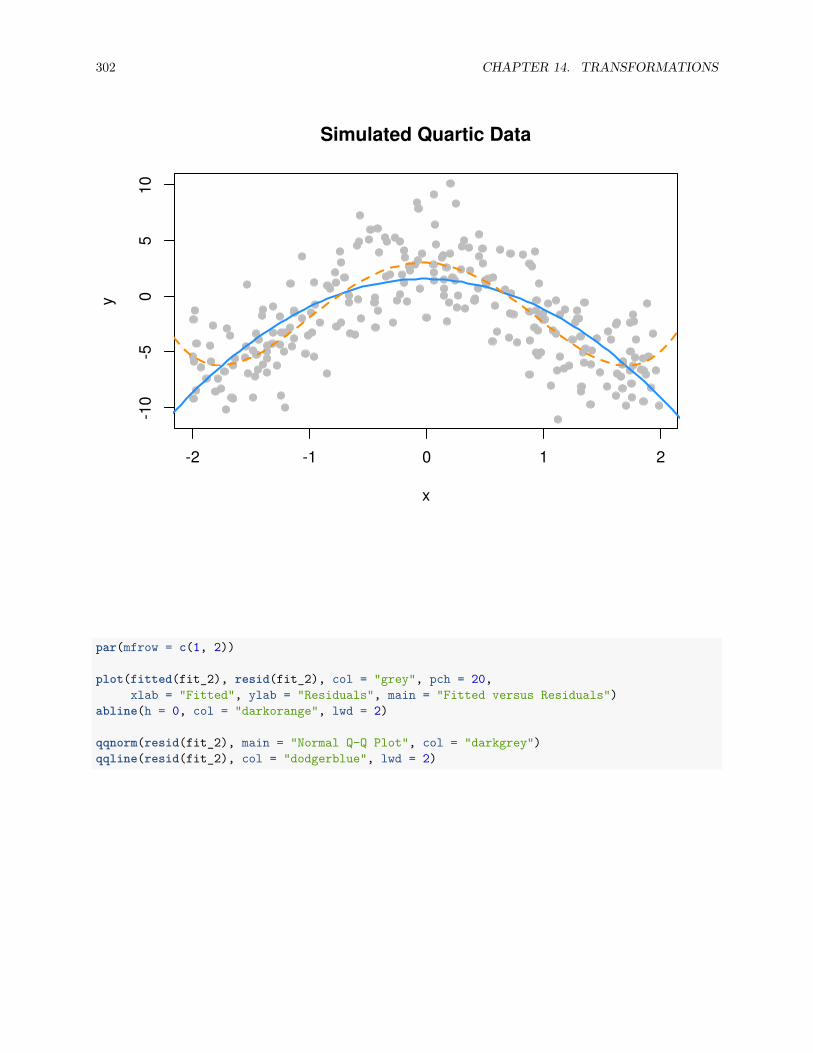
302 CHAPTER 14. TRANSFORMATIONS
-2 -1 0 1 2
-10
-50
510
Simulated Quartic Data
x
y
par(mfrow = c(1, 2))
plot(fitted(fit_2), resid(fit_2), col = "grey", pch = 20,xlab = "Fitted", ylab = "Residuals", main = "Fitted versus Residuals")
abline(h = 0, col = "darkorange", lwd = 2)
qqnorm(resid(fit_2), main = "Normal Q-Q Plot", col = "darkgrey")qqline(resid(fit_2), col = "dodgerblue", lwd = 2)
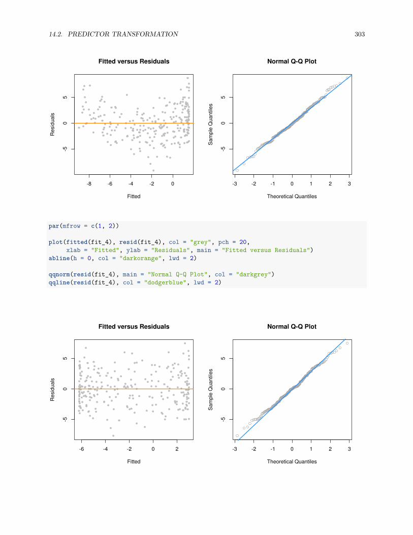
14.2. PREDICTOR TRANSFORMATION 303
-8 -6 -4 -2 0
-50
5Fitted versus Residuals
Fitted
Res
idua
ls
-3 -2 -1 0 1 2 3
-50
5
Normal Q-Q Plot
Theoretical Quantiles
Sam
ple
Qua
ntile
s
par(mfrow = c(1, 2))
plot(fitted(fit_4), resid(fit_4), col = "grey", pch = 20,xlab = "Fitted", ylab = "Residuals", main = "Fitted versus Residuals")
abline(h = 0, col = "darkorange", lwd = 2)
qqnorm(resid(fit_4), main = "Normal Q-Q Plot", col = "darkgrey")qqline(resid(fit_4), col = "dodgerblue", lwd = 2)
-6 -4 -2 0 2
-50
5
Fitted versus Residuals
Fitted
Res
idua
ls
-3 -2 -1 0 1 2 3
-50
5
Normal Q-Q Plot
Theoretical Quantiles
Sam
ple
Qua
ntile
s
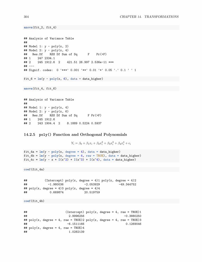
304 CHAPTER 14. TRANSFORMATIONS
anova(fit_2, fit_4)
## Analysis of Variance Table#### Model 1: y ~ poly(x, 2)## Model 2: y ~ poly(x, 4)## Res.Df RSS Df Sum of Sq F Pr(>F)## 1 247 2334.1## 2 245 1912.6 2 421.51 26.997 2.536e-11 ***## ---## Signif. codes: 0 '***' 0.001 '**' 0.01 '*' 0.05 '.' 0.1 ' ' 1
fit_6 = lm(y ~ poly(x, 6), data = data_higher)
anova(fit_4, fit_6)
## Analysis of Variance Table#### Model 1: y ~ poly(x, 4)## Model 2: y ~ poly(x, 6)## Res.Df RSS Df Sum of Sq F Pr(>F)## 1 245 1912.6## 2 243 1904.4 2 8.1889 0.5224 0.5937
14.2.5 poly() Function and Orthogonal Polynomials
Yi = β0 + β1xi + β2x2i + β3x3
i + β4x4i + ϵi
fit_4a = lm(y ~ poly(x, degree = 4), data = data_higher)fit_4b = lm(y ~ poly(x, degree = 4, raw = TRUE), data = data_higher)fit_4c = lm(y ~ x + I(x^2) + I(x^3) + I(x^4), data = data_higher)
coef(fit_4a)
## (Intercept) poly(x, degree = 4)1 poly(x, degree = 4)2## -1.980036 -2.053929 -49.344752## poly(x, degree = 4)3 poly(x, degree = 4)4## 0.669874 20.519759
coef(fit_4b)
## (Intercept) poly(x, degree = 4, raw = TRUE)1## 2.9996256 -0.3880250## poly(x, degree = 4, raw = TRUE)2 poly(x, degree = 4, raw = TRUE)3## -6.1511166 0.1269046## poly(x, degree = 4, raw = TRUE)4## 1.0282139

14.2. PREDICTOR TRANSFORMATION 305
coef(fit_4c)
## (Intercept) x I(x^2) I(x^3) I(x^4)## 2.9996256 -0.3880250 -6.1511166 0.1269046 1.0282139
unname(coef(fit_4a))
## [1] -1.980036 -2.053929 -49.344752 0.669874 20.519759
unname(coef(fit_4b))
## [1] 2.9996256 -0.3880250 -6.1511166 0.1269046 1.0282139
unname(coef(fit_4c))
## [1] 2.9996256 -0.3880250 -6.1511166 0.1269046 1.0282139
all.equal(fitted(fit_4a),fitted(fit_4b))
## [1] TRUE
all.equal(resid(fit_4a),resid(fit_4b))
## [1] TRUE
summary(fit_4a)
#### Call:## lm(formula = y ~ poly(x, degree = 4), data = data_higher)#### Residuals:## Min 1Q Median 3Q Max## -7.6982 -2.0334 0.0042 1.9532 7.4626#### Coefficients:## Estimate Std. Error t value Pr(>|t|)## (Intercept) -1.9800 0.1767 -11.205 < 2e-16 ***## poly(x, degree = 4)1 -2.0539 2.7940 -0.735 0.463## poly(x, degree = 4)2 -49.3448 2.7940 -17.661 < 2e-16 ***## poly(x, degree = 4)3 0.6699 2.7940 0.240 0.811## poly(x, degree = 4)4 20.5198 2.7940 7.344 3.06e-12 ***## ---## Signif. codes: 0 '***' 0.001 '**' 0.01 '*' 0.05 '.' 0.1 ' ' 1#### Residual standard error: 2.794 on 245 degrees of freedom## Multiple R-squared: 0.5993, Adjusted R-squared: 0.5928## F-statistic: 91.61 on 4 and 245 DF, p-value: < 2.2e-16
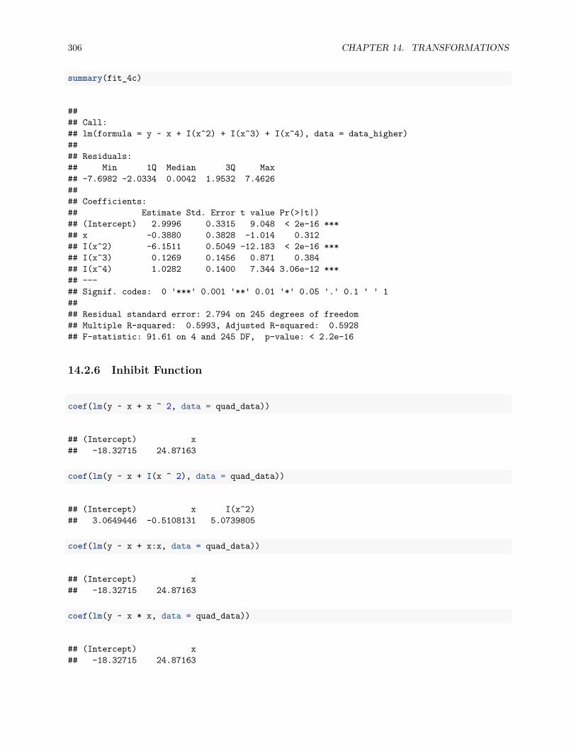
306 CHAPTER 14. TRANSFORMATIONS
summary(fit_4c)
#### Call:## lm(formula = y ~ x + I(x^2) + I(x^3) + I(x^4), data = data_higher)#### Residuals:## Min 1Q Median 3Q Max## -7.6982 -2.0334 0.0042 1.9532 7.4626#### Coefficients:## Estimate Std. Error t value Pr(>|t|)## (Intercept) 2.9996 0.3315 9.048 < 2e-16 ***## x -0.3880 0.3828 -1.014 0.312## I(x^2) -6.1511 0.5049 -12.183 < 2e-16 ***## I(x^3) 0.1269 0.1456 0.871 0.384## I(x^4) 1.0282 0.1400 7.344 3.06e-12 ***## ---## Signif. codes: 0 '***' 0.001 '**' 0.01 '*' 0.05 '.' 0.1 ' ' 1#### Residual standard error: 2.794 on 245 degrees of freedom## Multiple R-squared: 0.5993, Adjusted R-squared: 0.5928## F-statistic: 91.61 on 4 and 245 DF, p-value: < 2.2e-16
14.2.6 Inhibit Function
coef(lm(y ~ x + x ^ 2, data = quad_data))
## (Intercept) x## -18.32715 24.87163
coef(lm(y ~ x + I(x ^ 2), data = quad_data))
## (Intercept) x I(x^2)## 3.0649446 -0.5108131 5.0739805
coef(lm(y ~ x + x:x, data = quad_data))
## (Intercept) x## -18.32715 24.87163
coef(lm(y ~ x * x, data = quad_data))
## (Intercept) x## -18.32715 24.87163
14.2. PREDICTOR TRANSFORMATION 307
coef(lm(y ~ x ^ 2, data = quad_data))
## (Intercept) x## -18.32715 24.87163
coef(lm(y ~ x + x ^ 2, data = quad_data))
## (Intercept) x## -18.32715 24.87163
coef(lm(y ~ I(x + x), data = quad_data))
## (Intercept) I(x + x)## -18.32715 12.43582
coef(lm(y ~ x + x, data = quad_data))
## (Intercept) x## -18.32715 24.87163
14.2.7 Data Example
pairs(autompg)

308 CHAPTER 14. TRANSFORMATIONS
mpg
1.0 2.0 3.0 50 150 10 15 20 25 1.0 2.0 3.0
1030
1.0
2.0
3.0
cyl
disp
100
300
5015
0 hp
wt
1500
3500
1015
2025
acc
year
7074
7882
1.0
2.0
3.0
origin
10 30 100 300 1500 3500 70 74 78 82 0.0 0.4 0.80.
00.
40.
8
domestic
mpg_hp = lm(mpg ~ hp, data = autompg)
par(mfrow = c(1, 2))
plot(mpg ~ hp, data = autompg, col = "dodgerblue", pch = 20, cex = 1.5)abline(mpg_hp, col = "darkorange", lwd = 2)
plot(fitted(mpg_hp), resid(mpg_hp), col = "dodgerblue",pch = 20, cex = 1.5, xlab = "Fitted", ylab = "Residuals")
abline(h = 0, lty = 2, col = "darkorange", lwd = 2)
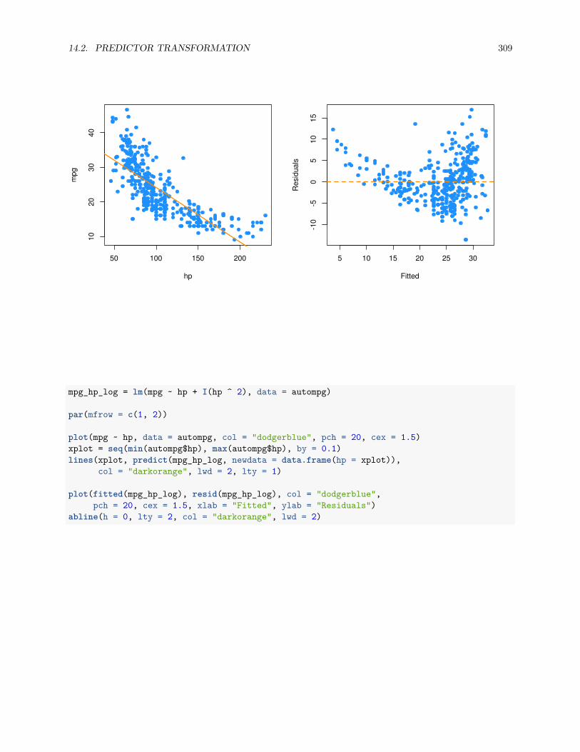
14.2. PREDICTOR TRANSFORMATION 309
50 100 150 200
1020
3040
hp
mpg
5 10 15 20 25 30
-10
-50
510
15
Fitted
Res
idua
ls
mpg_hp_log = lm(mpg ~ hp + I(hp ^ 2), data = autompg)
par(mfrow = c(1, 2))
plot(mpg ~ hp, data = autompg, col = "dodgerblue", pch = 20, cex = 1.5)xplot = seq(min(autompg$hp), max(autompg$hp), by = 0.1)lines(xplot, predict(mpg_hp_log, newdata = data.frame(hp = xplot)),
col = "darkorange", lwd = 2, lty = 1)
plot(fitted(mpg_hp_log), resid(mpg_hp_log), col = "dodgerblue",pch = 20, cex = 1.5, xlab = "Fitted", ylab = "Residuals")
abline(h = 0, lty = 2, col = "darkorange", lwd = 2)
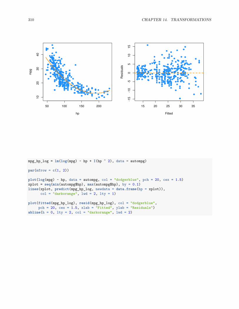
310 CHAPTER 14. TRANSFORMATIONS
50 100 150 200
1020
3040
hp
mpg
15 20 25 30 35
-15
-10
-50
510
15
Fitted
Res
idua
ls
mpg_hp_log = lm(log(mpg) ~ hp + I(hp ^ 2), data = autompg)
par(mfrow = c(1, 2))
plot(log(mpg) ~ hp, data = autompg, col = "dodgerblue", pch = 20, cex = 1.5)xplot = seq(min(autompg$hp), max(autompg$hp), by = 0.1)lines(xplot, predict(mpg_hp_log, newdata = data.frame(hp = xplot)),
col = "darkorange", lwd = 2, lty = 1)
plot(fitted(mpg_hp_log), resid(mpg_hp_log), col = "dodgerblue",pch = 20, cex = 1.5, xlab = "Fitted", ylab = "Residuals")
abline(h = 0, lty = 2, col = "darkorange", lwd = 2)
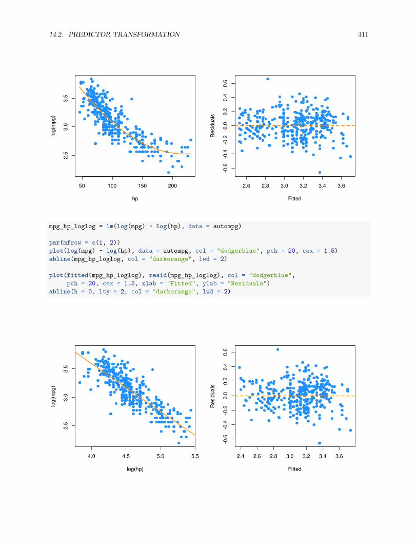
14.2. PREDICTOR TRANSFORMATION 311
50 100 150 200
2.5
3.0
3.5
hp
log(
mpg
)
2.6 2.8 3.0 3.2 3.4 3.6
-0.6
-0.4
-0.2
0.0
0.2
0.4
0.6
Fitted
Res
idua
ls
mpg_hp_loglog = lm(log(mpg) ~ log(hp), data = autompg)
par(mfrow = c(1, 2))plot(log(mpg) ~ log(hp), data = autompg, col = "dodgerblue", pch = 20, cex = 1.5)abline(mpg_hp_loglog, col = "darkorange", lwd = 2)
plot(fitted(mpg_hp_loglog), resid(mpg_hp_loglog), col = "dodgerblue",pch = 20, cex = 1.5, xlab = "Fitted", ylab = "Residuals")
abline(h = 0, lty = 2, col = "darkorange", lwd = 2)
4.0 4.5 5.0 5.5
2.5
3.0
3.5
log(hp)
log(
mpg
)
2.4 2.6 2.8 3.0 3.2 3.4 3.6
-0.6
-0.4
-0.2
0.0
0.2
0.4
0.6
Fitted
Res
idua
ls
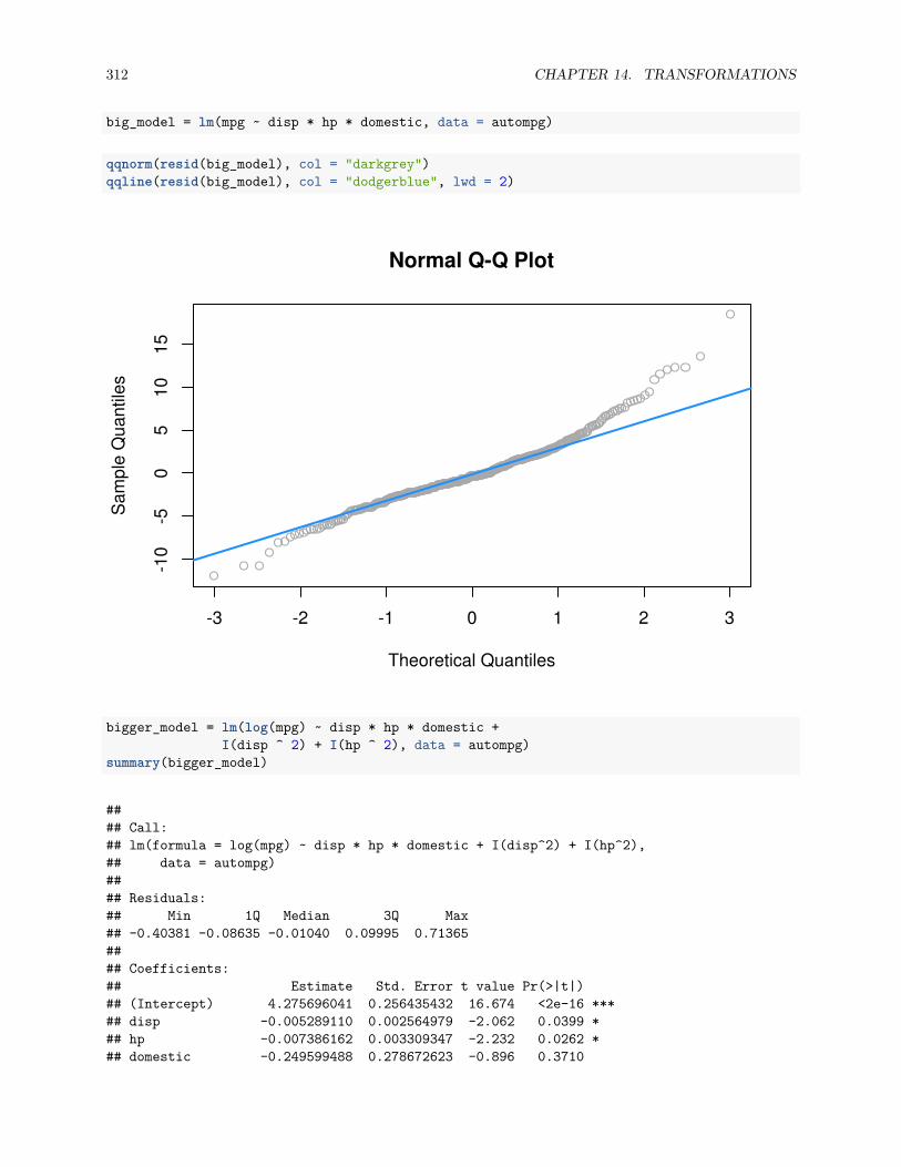
312 CHAPTER 14. TRANSFORMATIONS
big_model = lm(mpg ~ disp * hp * domestic, data = autompg)
qqnorm(resid(big_model), col = "darkgrey")qqline(resid(big_model), col = "dodgerblue", lwd = 2)
-3 -2 -1 0 1 2 3
-10
-50
510
15
Normal Q-Q Plot
Theoretical Quantiles
Sam
ple
Qua
ntile
s
bigger_model = lm(log(mpg) ~ disp * hp * domestic +I(disp ^ 2) + I(hp ^ 2), data = autompg)
summary(bigger_model)
#### Call:## lm(formula = log(mpg) ~ disp * hp * domestic + I(disp^2) + I(hp^2),## data = autompg)#### Residuals:## Min 1Q Median 3Q Max## -0.40381 -0.08635 -0.01040 0.09995 0.71365#### Coefficients:## Estimate Std. Error t value Pr(>|t|)## (Intercept) 4.275696041 0.256435432 16.674 <2e-16 ***## disp -0.005289110 0.002564979 -2.062 0.0399 *## hp -0.007386162 0.003309347 -2.232 0.0262 *## domestic -0.249599488 0.278672623 -0.896 0.3710
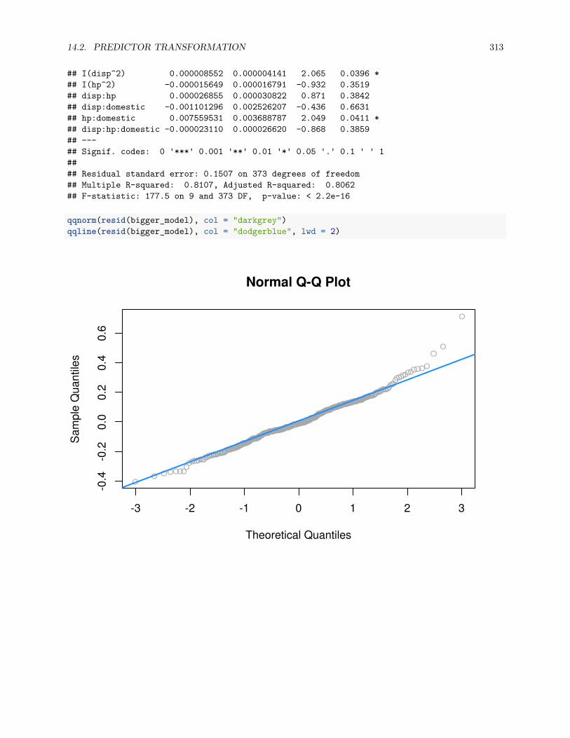
14.2. PREDICTOR TRANSFORMATION 313
## I(disp^2) 0.000008552 0.000004141 2.065 0.0396 *## I(hp^2) -0.000015649 0.000016791 -0.932 0.3519## disp:hp 0.000026855 0.000030822 0.871 0.3842## disp:domestic -0.001101296 0.002526207 -0.436 0.6631## hp:domestic 0.007559531 0.003688787 2.049 0.0411 *## disp:hp:domestic -0.000023110 0.000026620 -0.868 0.3859## ---## Signif. codes: 0 '***' 0.001 '**' 0.01 '*' 0.05 '.' 0.1 ' ' 1#### Residual standard error: 0.1507 on 373 degrees of freedom## Multiple R-squared: 0.8107, Adjusted R-squared: 0.8062## F-statistic: 177.5 on 9 and 373 DF, p-value: < 2.2e-16
qqnorm(resid(bigger_model), col = "darkgrey")qqline(resid(bigger_model), col = "dodgerblue", lwd = 2)
-3 -2 -1 0 1 2 3
-0.4
-0.2
0.0
0.2
0.4
0.6
Normal Q-Q Plot
Theoretical Quantiles
Sam
ple
Qua
ntile
s

314 CHAPTER 14. TRANSFORMATIONS

Chapter 15
Collinearity
“If I look confused it is because I am thinking.”— Samuel Goldwyn
After reading this chapter you will be able to:
• Identify collinearity in regression.• Understand the effect of collinearity on regression models.
15.1 Exact Collinearity
Let’s create a dataset where one of the predictors, x3, is a linear combination of the other predictors.
gen_exact_collin_data = function(num_samples = 100) {x1 = rnorm(n = num_samples, mean = 80, sd = 10)x2 = rnorm(n = num_samples, mean = 70, sd = 5)x3 = 2 * x1 + 4 * x2 + 3y = 3 + x1 + x2 + rnorm(n = num_samples, mean = 0, sd = 1)data.frame(y, x1, x2, x3)
}
Notice that the way we are generating this data, the response y only really depends on x1 and x2.
set.seed(42)exact_collin_data = gen_exact_collin_data()head(exact_collin_data)
## y x1 x2 x3## 1 170.7135 93.70958 76.00483 494.4385## 2 152.9106 74.35302 75.22376 452.6011## 3 152.7866 83.63128 64.98396 430.1984## 4 170.6306 86.32863 79.24241 492.6269## 5 152.3320 84.04268 66.66613 437.7499## 6 151.3155 78.93875 70.52757 442.9878
315

316 CHAPTER 15. COLLINEARITY
What happens when we attempt to fit a regression model in R using all of the predictors?
exact_collin_fit = lm(y ~ x1 + x2 + x3, data = exact_collin_data)summary(exact_collin_fit)
#### Call:## lm(formula = y ~ x1 + x2 + x3, data = exact_collin_data)#### Residuals:## Min 1Q Median 3Q Max## -2.57662 -0.66188 -0.08253 0.63706 2.52057#### Coefficients: (1 not defined because of singularities)## Estimate Std. Error t value Pr(>|t|)## (Intercept) 2.957336 1.735165 1.704 0.0915 .## x1 0.985629 0.009788 100.702 <2e-16 ***## x2 1.017059 0.022545 45.112 <2e-16 ***## x3 NA NA NA NA## ---## Signif. codes: 0 '***' 0.001 '**' 0.01 '*' 0.05 '.' 0.1 ' ' 1#### Residual standard error: 1.014 on 97 degrees of freedom## Multiple R-squared: 0.9923, Adjusted R-squared: 0.9921## F-statistic: 6236 on 2 and 97 DF, p-value: < 2.2e-16
We see that R simply decides to exclude a variable. Why is this happening?
X = cbind(1, as.matrix(exact_collin_data[,-1]))solve(t(X) %*% X)
If we attempt to find β using(
XT X)−1
, we see that this is not possible, due to the fact that the columnsof X are linearly dependent. The previous lines of code were not run, because they produce an error!
When this happens, we say there is exact collinearity in the dataset.
As a result of this issue, R essentially chose to fit the model y ~ x1 + x2. However notice that two othermodels would accomplish exactly the same fit.
fit1 = lm(y ~ x1 + x2, data = exact_collin_data)fit2 = lm(y ~ x1 + x3, data = exact_collin_data)fit3 = lm(y ~ x2 + x3, data = exact_collin_data)
We see that the fitted values for each of the three models are exactly the same. This is a result of x3containing all of the information from x1 and x2. As long as one of x1 or x2 are included in the model, x3can be used to recover the information from the variable not included.
all.equal(fitted(fit1), fitted(fit2))
## [1] TRUE

15.2. COLLINEARITY 317
all.equal(fitted(fit2), fitted(fit3))
## [1] TRUE
While their fitted values are all the same, their estimated coefficients are wildly different. The sign of x2 isswitched in two of the models! So only fit1 properly explains the relationship between the variables, fit2and fit3 still predict as well as fit1, despite the coefficients having little to no meaning, a concept we willreturn to later.
coef(fit1)
## (Intercept) x1 x2## 2.9573357 0.9856291 1.0170586
coef(fit2)
## (Intercept) x1 x3## 2.1945418 0.4770998 0.2542647
coef(fit3)
## (Intercept) x2 x3## 1.4788921 -0.9541995 0.4928145
15.2 Collinearity
Exact collinearity is an extreme example of collinearity, which occurs in multiple regression when predictorvariables are highly correlated. Collinearity is often called multicollinearity, since it is a phenomenon thatreally only occurs during multiple regression.
Looking at the seatpos dataset from the faraway package, we will see an example of this concept. Thepredictors in this dataset are various attributes of car drivers, such as their height, weight and age. Theresponse variable hipcenter measures the “horizontal distance of the midpoint of the hips from a fixedlocation in the car in mm.” Essentially, it measures the position of the seat for a given driver. This ispotentially useful information for car manufacturers considering comfort and safety when designing vehicles.
We will attempt to fit a model that predicts hipcenter. Two predictor variables are immediately interestingto us: HtShoes and Ht. We certainly expect a person’s height to be highly correlated to their height whenwearing shoes. We’ll pay special attention to these two variables when fitting models.
library(faraway)pairs(seatpos, col = "dodgerblue")

318 CHAPTER 15. COLLINEARITY
Age
100 200 300 150 180 26 32 38 30 36 42
2040
60
100
200
300
Weight
HtShoes
160
190
150
180
Ht
Seated
8090
100
2632
38
Arm
Thigh
3545
3036
42
Leg
20 40 60 160 190 80 90 100 35 45 -250 -100-2
50-1
00
hipcenter
round(cor(seatpos), 2)
## Age Weight HtShoes Ht Seated Arm Thigh Leg hipcenter## Age 1.00 0.08 -0.08 -0.09 -0.17 0.36 0.09 -0.04 0.21## Weight 0.08 1.00 0.83 0.83 0.78 0.70 0.57 0.78 -0.64## HtShoes -0.08 0.83 1.00 1.00 0.93 0.75 0.72 0.91 -0.80## Ht -0.09 0.83 1.00 1.00 0.93 0.75 0.73 0.91 -0.80## Seated -0.17 0.78 0.93 0.93 1.00 0.63 0.61 0.81 -0.73## Arm 0.36 0.70 0.75 0.75 0.63 1.00 0.67 0.75 -0.59## Thigh 0.09 0.57 0.72 0.73 0.61 0.67 1.00 0.65 -0.59## Leg -0.04 0.78 0.91 0.91 0.81 0.75 0.65 1.00 -0.79## hipcenter 0.21 -0.64 -0.80 -0.80 -0.73 -0.59 -0.59 -0.79 1.00
After loading the faraway package, we do some quick checks of correlation between the predictors. Visually,

15.2. COLLINEARITY 319
we can do this with the pairs() function, which plots all possible scatterplots between pairs of variables inthe dataset.
We can also do this numerically with the cor() function, which when applied to a dataset, returns all pairwisecorrelations. Notice this is a symmetric matrix. Recall that correlation measures strength and direction ofthe linear relationship between to variables. The correlation between Ht and HtShoes is extremely high. Sohigh, that rounded to two decimal places, it appears to be 1!
Unlike exact collinearity, here we can still fit a model with all of the predictors, but what effect does thishave?
hip_model = lm(hipcenter ~ ., data = seatpos)summary(hip_model)
#### Call:## lm(formula = hipcenter ~ ., data = seatpos)#### Residuals:## Min 1Q Median 3Q Max## -73.827 -22.833 -3.678 25.017 62.337#### Coefficients:## Estimate Std. Error t value Pr(>|t|)## (Intercept) 436.43213 166.57162 2.620 0.0138 *## Age 0.77572 0.57033 1.360 0.1843## Weight 0.02631 0.33097 0.080 0.9372## HtShoes -2.69241 9.75304 -0.276 0.7845## Ht 0.60134 10.12987 0.059 0.9531## Seated 0.53375 3.76189 0.142 0.8882## Arm -1.32807 3.90020 -0.341 0.7359## Thigh -1.14312 2.66002 -0.430 0.6706## Leg -6.43905 4.71386 -1.366 0.1824## ---## Signif. codes: 0 '***' 0.001 '**' 0.01 '*' 0.05 '.' 0.1 ' ' 1#### Residual standard error: 37.72 on 29 degrees of freedom## Multiple R-squared: 0.6866, Adjusted R-squared: 0.6001## F-statistic: 7.94 on 8 and 29 DF, p-value: 0.00001306
One of the first things we should notice is that the F -test for the regression tells us that the regressionis significant, however each individual predictor is not. Another interesting result is the opposite signs ofthe coefficients for Ht and HtShoes. This should seem rather counter-intuitive. Increasing Ht increaseshipcenter, but increasing HtShoes decreases hipcenter?
This happens as a result of the predictors being highly correlated. For example, the HtShoe variable explainsa large amount of the variation in Ht. When they are both in the model, their effects on the response arelessened individually, but together they still explain a large portion of the variation of hipcenter.
We define R2j to be the proportion of observed variation in the j-th predictor explained by the other predictors.
In other words R2j is the multiple R-Squared for the regression of xj on each of the other predictors.
ht_shoes_model = lm(HtShoes ~ . - hipcenter, data = seatpos)summary(ht_shoes_model)$r.squared
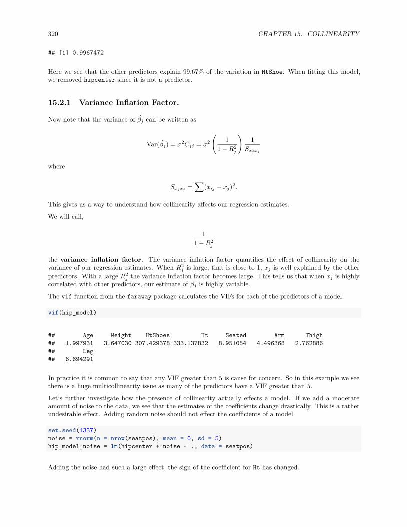
320 CHAPTER 15. COLLINEARITY
## [1] 0.9967472
Here we see that the other predictors explain 99.67% of the variation in HtShoe. When fitting this model,we removed hipcenter since it is not a predictor.
15.2.1 Variance Inflation Factor.
Now note that the variance of βj can be written as
Var(βj) = σ2Cjj = σ2
(1
1 − R2j
)1
Sxjxj
where
Sxjxj=∑
(xij − xj)2.
This gives us a way to understand how collinearity affects our regression estimates.
We will call,
11 − R2
j
the variance inflation factor. The variance inflation factor quantifies the effect of collinearity on thevariance of our regression estimates. When R2
j is large, that is close to 1, xj is well explained by the otherpredictors. With a large R2
j the variance inflation factor becomes large. This tells us that when xj is highlycorrelated with other predictors, our estimate of βj is highly variable.
The vif function from the faraway package calculates the VIFs for each of the predictors of a model.
vif(hip_model)
## Age Weight HtShoes Ht Seated Arm Thigh## 1.997931 3.647030 307.429378 333.137832 8.951054 4.496368 2.762886## Leg## 6.694291
In practice it is common to say that any VIF greater than 5 is cause for concern. So in this example we seethere is a huge multicollinearity issue as many of the predictors have a VIF greater than 5.
Let’s further investigate how the presence of collinearity actually effects a model. If we add a moderateamount of noise to the data, we see that the estimates of the coefficients change drastically. This is a ratherundesirable effect. Adding random noise should not effect the coefficients of a model.
set.seed(1337)noise = rnorm(n = nrow(seatpos), mean = 0, sd = 5)hip_model_noise = lm(hipcenter + noise ~ ., data = seatpos)
Adding the noise had such a large effect, the sign of the coefficient for Ht has changed.
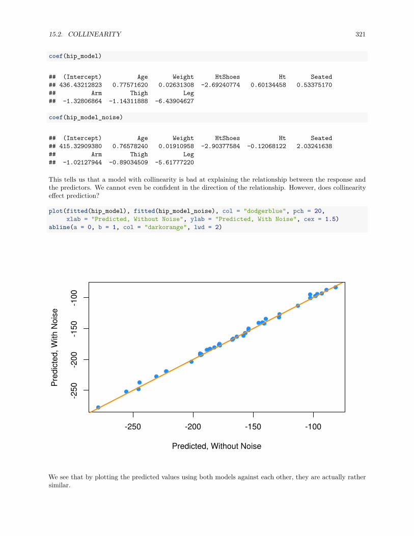
15.2. COLLINEARITY 321
coef(hip_model)
## (Intercept) Age Weight HtShoes Ht Seated## 436.43212823 0.77571620 0.02631308 -2.69240774 0.60134458 0.53375170## Arm Thigh Leg## -1.32806864 -1.14311888 -6.43904627
coef(hip_model_noise)
## (Intercept) Age Weight HtShoes Ht Seated## 415.32909380 0.76578240 0.01910958 -2.90377584 -0.12068122 2.03241638## Arm Thigh Leg## -1.02127944 -0.89034509 -5.61777220
This tells us that a model with collinearity is bad at explaining the relationship between the response andthe predictors. We cannot even be confident in the direction of the relationship. However, does collinearityeffect prediction?
plot(fitted(hip_model), fitted(hip_model_noise), col = "dodgerblue", pch = 20,xlab = "Predicted, Without Noise", ylab = "Predicted, With Noise", cex = 1.5)
abline(a = 0, b = 1, col = "darkorange", lwd = 2)
-250 -200 -150 -100
-250
-200
-150
-100
Predicted, Without Noise
Pre
dict
ed, W
ith N
oise
We see that by plotting the predicted values using both models against each other, they are actually rathersimilar.

322 CHAPTER 15. COLLINEARITY
Let’s now look at a smaller model,
hip_model_small = lm(hipcenter ~ Age + Arm + Ht, data = seatpos)summary(hip_model_small)
#### Call:## lm(formula = hipcenter ~ Age + Arm + Ht, data = seatpos)#### Residuals:## Min 1Q Median 3Q Max## -82.347 -24.745 -0.094 23.555 58.314#### Coefficients:## Estimate Std. Error t value Pr(>|t|)## (Intercept) 493.2491 101.0724 4.880 0.0000246 ***## Age 0.7988 0.5111 1.563 0.12735## Arm -2.9385 3.5210 -0.835 0.40979## Ht -3.4991 0.9954 -3.515 0.00127 **## ---## Signif. codes: 0 '***' 0.001 '**' 0.01 '*' 0.05 '.' 0.1 ' ' 1#### Residual standard error: 36.12 on 34 degrees of freedom## Multiple R-squared: 0.6631, Adjusted R-squared: 0.6333## F-statistic: 22.3 on 3 and 34 DF, p-value: 0.00000003649
vif(hip_model_small)
## Age Arm Ht## 1.749943 3.996766 3.508693
Immediately we see that multicollinearity isn’t an issue here.
anova(hip_model_small, hip_model)
## Analysis of Variance Table#### Model 1: hipcenter ~ Age + Arm + Ht## Model 2: hipcenter ~ Age + Weight + HtShoes + Ht + Seated + Arm + Thigh +## Leg## Res.Df RSS Df Sum of Sq F Pr(>F)## 1 34 44354## 2 29 41262 5 3091.9 0.4346 0.8207
Also notice that using an F -test to compare the two models, we would prefer the smaller model.
We now investigate the effect of adding another variable to this smaller model. Specifically we want to lookat adding the variable HtShoes. So now our possible predictors are HtShoes, Age, Arm, and Ht. Our responseis still hipcenter.
To quantify this effect we will look at a variable added plot and a partial correlation coefficient. Forboth of these, we will look at the residuals of two models:

15.2. COLLINEARITY 323
• Regressing the response (hipcenter) against all of the predictors except the predictor of interest(HtShoes).
• Regressing the predictor of interest (HtShoes) against the other predictors (Age, Arm, and Ht).
ht_shoes_model_small = lm(HtShoes ~ Age + Arm + Ht, data = seatpos)
So now, the residuals of hip_model_small give us the variation of hipcenter that is unexplained by Age,Arm, and Ht. Similarly, the residuals of ht_shoes_model_small give us the variation of HtShoes unexplainedby Age, Arm, and Ht.
The correlation of these two residuals gives us the partial correlation coefficient of HtShoes andhipcenter with the effects of Age, Arm, and Ht removed.
cor(resid(ht_shoes_model_small), resid(hip_model_small))
## [1] -0.03311061
Since this value is small, close to zero, it means that the variation of hipcenter that is unexplained by Age,Arm, and Ht shows very little correlation with the variation of HtShoes that is not explained by Age, Arm,and Ht. Thus adding HtShoes to the model would likely be of little benefit.
Similarly a variable added plot visualizes these residuals against each other. It is also helpful to regressthe residuals of the response against the residuals of the predictor and add the regression line to the plot.
plot(resid(hip_model_small) ~ resid(ht_shoes_model_small),col = "dodgerblue", pch = 20,xlab = "Residuals, Added Predictor",ylab = "Residuals, Original Model")
abline(h = 0, lty = 2)abline(v = 0, lty = 2)abline(lm(resid(hip_model_small) ~ resid(ht_shoes_model_small)),
col = "darkorange", lwd = 2)
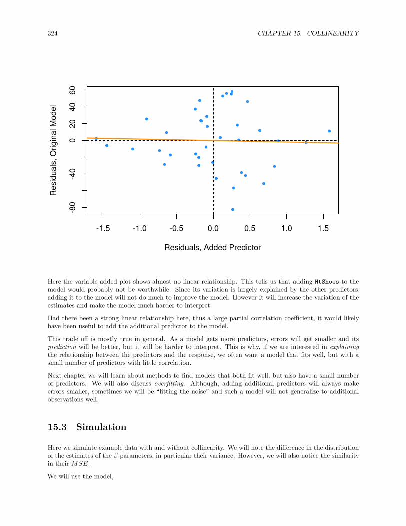
324 CHAPTER 15. COLLINEARITY
-1.5 -1.0 -0.5 0.0 0.5 1.0 1.5
-80
-40
020
4060
Residuals, Added Predictor
Res
idua
ls, O
rigin
al M
odel
Here the variable added plot shows almost no linear relationship. This tells us that adding HtShoes to themodel would probably not be worthwhile. Since its variation is largely explained by the other predictors,adding it to the model will not do much to improve the model. However it will increase the variation of theestimates and make the model much harder to interpret.
Had there been a strong linear relationship here, thus a large partial correlation coefficient, it would likelyhave been useful to add the additional predictor to the model.
This trade off is mostly true in general. As a model gets more predictors, errors will get smaller and itsprediction will be better, but it will be harder to interpret. This is why, if we are interested in explainingthe relationship between the predictors and the response, we often want a model that fits well, but with asmall number of predictors with little correlation.
Next chapter we will learn about methods to find models that both fit well, but also have a small numberof predictors. We will also discuss overfitting. Although, adding additional predictors will always makeerrors smaller, sometimes we will be “fitting the noise” and such a model will not generalize to additionalobservations well.
15.3 Simulation
Here we simulate example data with and without collinearity. We will note the difference in the distributionof the estimates of the β parameters, in particular their variance. However, we will also notice the similarityin their MSE.
We will use the model,

15.3. SIMULATION 325
Y = β0 + β1x1 + β2x2 + ϵ
where ϵ ∼ N(µ = 0, σ2 = 25) and the β coefficients defined below.
set.seed(42)beta_0 = 7beta_1 = 3beta_2 = 4sigma = 5
We will use a sample size of 10, and 2500 simulations for both situations.
sample_size = 10num_sim = 2500
We’ll first consider the situation with a collinearity issue, so we manually create the two predictor variables.
x1 = c(1, 2, 3, 4, 5, 6, 7, 8, 9, 10)x2 = c(1, 2, 3, 4, 5, 7, 6, 10, 9, 8)
c(sd(x1), sd(x2))
## [1] 3.02765 3.02765
cor(x1, x2)
## [1] 0.9393939
Notice that they have extremely high correlation.
true_line_bad = beta_0 + beta_1 * x1 + beta_2 * x2beta_hat_bad = matrix(0, num_sim, 2)mse_bad = rep(0, num_sim)
We perform the simulation 2500 times, each time fitting a regression model, and storing the estimatedcoefficients and the MSE.
for (s in 1:num_sim) {y = true_line_bad + rnorm(n = sample_size, mean = 0, sd = sigma)reg_out = lm(y ~ x1 + x2)beta_hat_bad[s, ] = coef(reg_out)[-1]mse_bad[s] = mean(resid(reg_out) ^ 2)
}
Now we move to the situation without a collinearity issue, so we again manually create the two predictorvariables.

326 CHAPTER 15. COLLINEARITY
z1 = c(1, 2, 3, 4, 5, 6, 7, 8, 9, 10)z2 = c(9, 2, 7, 4, 5, 6, 3, 8, 1, 10)
Notice that the standard deviations of each are the same as before, however, now the correlation is extremelyclose to 0.
c(sd(z1), sd(z2))
## [1] 3.02765 3.02765
cor(z1, z2)
## [1] 0.03030303
true_line_good = beta_0 + beta_1 * z1 + beta_2 * z2beta_hat_good = matrix(0, num_sim, 2)mse_good = rep(0, num_sim)
We then perform simulations and store the same results.
for (s in 1:num_sim) {y = true_line_good + rnorm(n = sample_size, mean = 0, sd = sigma)reg_out = lm(y ~ z1 + z2)beta_hat_good[s, ] = coef(reg_out)[-1]mse_good[s] = mean(resid(reg_out) ^ 2)
}
We’ll now investigate the differences.
par(mfrow = c(1, 2))hist(beta_hat_bad[, 1],
col = "darkorange",border = "dodgerblue",main = expression("Histogram of " *hat(beta)[1]* " with Collinearity"),xlab = expression(hat(beta)[1]),breaks = 20)
hist(beta_hat_good[, 1],col = "darkorange",border = "dodgerblue",main = expression("Histogram of " *hat(beta)[1]* " without Collinearity"),xlab = expression(hat(beta)[1]),breaks = 20)

15.3. SIMULATION 327
Histogram of β1 with Collinearity
β1
Freq
uenc
y
-2 0 2 4 6 8 10
050
100
150
200
250
300
Histogram of β1 without Collinearity
β1
Freq
uenc
y
1 2 3 4 5
010
020
030
0First, for β1, which has a true value of 3, we see that both with and without collinearity, the simulated valuesare centered near 3.
mean(beta_hat_bad[, 1])
## [1] 2.963325
mean(beta_hat_good[, 1])
## [1] 3.013414
The way the predictors were created, the Sxjxjportion of the variance is the same for the predictors in both
cases, but the variance is still much larger in the simulations performed with collinearity. The variance is solarge in the collinear case, that sometimes the estimated coefficient for β1 is negative!
sd(beta_hat_bad[, 1])
## [1] 1.633294
sd(beta_hat_good[, 1])
## [1] 0.5484684
par(mfrow = c(1, 2))hist(beta_hat_bad[, 2],
col = "darkorange",border = "dodgerblue",main = expression("Histogram of " *hat(beta)[2]* " with Collinearity"),xlab = expression(hat(beta)[2]),

328 CHAPTER 15. COLLINEARITY
breaks = 20)hist(beta_hat_good[, 2],
col = "darkorange",border = "dodgerblue",main = expression("Histogram of " *hat(beta)[2]* " without Collinearity"),xlab = expression(hat(beta)[2]),breaks = 20)
Histogram of β2 with Collinearity
β2
Freq
uenc
y
-2 0 2 4 6 8 10
050
100
150
200
250
300
Histogram of β2 without Collinearity
β2
Freq
uenc
y
2 3 4 5 6
010
020
030
040
0
We see the same issues with β2. On average the estimates are correct, but the variance is again much largerwith collinearity.
mean(beta_hat_bad[, 2])
## [1] 4.025059
mean(beta_hat_good[, 2])
## [1] 4.004913
sd(beta_hat_bad[, 2])
## [1] 1.642592
sd(beta_hat_good[, 2])
## [1] 0.5470381

15.3. SIMULATION 329
par(mfrow = c(1, 2))hist(mse_bad,
col = "darkorange",border = "dodgerblue",main = "MSE, with Collinearity",xlab = "MSE")
hist(mse_good,col = "darkorange",border = "dodgerblue",main = "MSE, without Collinearity",xlab = "MSE")
MSE, with Collinearity
MSE
Freq
uenc
y
0 20 40 60
010
020
030
040
050
060
0
MSE, without Collinearity
MSE
Freq
uenc
y
0 10 20 30 40 50 60 70
010
020
030
040
050
060
0
Interestingly, in both cases, the MSE is roughly the same on average. Again, this is because collinearityeffects a model’s ability to explain, but not predict.
mean(mse_bad)
## [1] 17.7186
mean(mse_good)
## [1] 17.70513

330 CHAPTER 15. COLLINEARITY

Chapter 16
Variable Selection and ModelBuilding
“Choose well. Your choice is brief, and yet endless.”
— Johann Wolfgang von Goethe
After reading this chapter you will be able to:
• Understand the trade-off between goodness-of-fit and model complexity.• Use variable selection procedures to find a good model from a set of possible models.• Understand the two uses of models: explanation and prediction.
Last chapter we saw how correlation between predictor variables can have undesirable effects on models. Weused variance inflation factors to assess the severity of the collinearity issues caused by these correlations.We also saw how fitting a smaller model, leaving out some of the correlated predictors, results in a modelwhich no longer suffers from collinearity issues. But how should we chose this smaller model?
This chapter, we will discuss several criteria and procedures for choosing a “good” model from among achoice of many.
16.1 Quality Criterion
So far, we have seen criteria such as R2 and RMSE for assessing quality of fit. However, both of these havea fatal flaw. By increasing the size of a model, that is adding predictors, that can at worst not improve. Itis impossible to add a predictor to a model and make R2 or RMSE worse. That means, if we were to useeither of these to chose between models, we would always simply choose the larger model. Eventually wewould simply be fitting to noise.
This suggests that we need a quality criteria that takes into account the size of the model, since our preferenceis for small models that still fit well. We are willing to sacrifice a small amount of “goodness-of-fit” forobtaining a smaller model. (Here we use “goodness-of-fit” to simply mean how far the data is from the model,the smaller the errors the better. Often in statistics, goodness-of-fit can have a more precise meaning.) Wewill look at three criteria that do this explicitly: AIC, BIC, and Adjusted R2. We will also look at one,Cross-Validated RMSE, which implicitly considers the size of the model.
331

332 CHAPTER 16. VARIABLE SELECTION AND MODEL BUILDING
16.1.1 Akaike Information Criterion
The first criteria we will discuss is the Akaike Information Criterion, or AIC for short. (Note that, whenAkaike first introduced this metric, it was simply called An Information Criterion. The A has changedmeaning over the years.)
Recall, the maximized log-likelihood of a regression model can be written as
log L(β, σ2) = −n
2log(2π) − n
2log(
RSSn
)− n
2,
where RSS =∑n
i=1(yi − yi)2 and β and σ2 were chosen to maximize the likelihood.
Then we can define AIC as
AIC = −2 log L(β, σ2) + 2p = n + n log(2π) + n log(
RSSn
)+ 2p,
which is a measure of quality of the model. The smaller the AIC, the better. To see why, let’s talk about thetwo main components of AIC, the likelihood (which measures “goodness-of-fit”) and the penalty (whichis a function of the size of the model).
The likelihood portion of AIC is given by
−2 log L(β, σ2) = n + n log(2π) + n log(
RSSn
).
For the sake of comparing models, the only term here that will change is n log(RSS
n
), which is function of
RSS. The
n + n log(2π)
terms will be constant across all models applied to the same data. So, when a model fits well, that is, has alow RSS, then this likelihood component will be small.
Similarly, we can discuss the penalty component of AIC which is,
2p,
where p is the number of β parameters in the model. We call this a penalty, because it is large when p islarge, but we are seeking to find a small AIC
Thus, a good model, that is one with a small AIC, will have a good balance between fitting well, and usinga small number of parameters. For comparing models
AIC = n log(
RSSn
)+ 2p
is a sufficient expression, as n + n log(2π) is the same across all models for any particular dataset.

16.1. QUALITY CRITERION 333
16.1.2 Bayesian Information Criterion
The Bayesian Information Criterion, or BIC, is similar to AIC, but has a larger penalty. BIC also quantifiesthe trade-off between a model which fits well and the number of model parameters, however for a reasonablesample size, generally picks a smaller model than AIC. Again, for model selection use the model with thesmallest BIC.
BIC = −2 log L(β, σ2) + log(n)p = n + n log(2π) + n log(
RSSn
)+ log(n)p.
Notice that the AIC penalty was
2p,
whereas for BIC, the penalty is
log(n)p.
So, for any dataset where log(n) > 2 the BIC penalty will be larger than the AIC penalty, thus BIC willlikely prefer a smaller model.
Note that, sometimes the penalty is considered a general expression of the form
k · p.
Then, for AIC k = 2, and for BIC k = log(n).
For comparing models
BIC = n log(
RSSn
)+ log(n)p
is again a sufficient expression, as n + n log(2π) is the same across all models for any particular dataset.
16.1.3 Adjusted R-Squared
Recall,
R2 = 1 − SSESST = 1 −
∑ni=1(yi − yi)2∑ni=1(yi − y)2 .
We now define
R2a = 1 − SSE/(n − p)
SST/(n − 1)= 1 −
(n − 1n − p
)(1 − R2)
which we call the Adjusted R2.
Unlike R2 which can never become smaller with added predictors, Adjusted R2 effectively penalizes foradditional predictors, and can decrease with added predictors. Like R2, larger is still better.

334 CHAPTER 16. VARIABLE SELECTION AND MODEL BUILDING
16.1.4 Cross-Validated RMSE
Each of the previous three metrics explicitly used p, the number of parameters, in their calculations. Thus,they all explicitly limit the size of models chosen when used to compare models.
We’ll now briefly introduce overfitting and cross-validation.
make_poly_data = function(sample_size = 11) {x = seq(0, 10)y = 3 + x + 4 * x ^ 2 + rnorm(n = sample_size, mean = 0, sd = 20)data.frame(x, y)
}
set.seed(1234)poly_data = make_poly_data()
Here we have generated data where the mean of Y is a quadratic function of a single predictor x, specifically,
Y = 3 + x + 4x2 + ϵ.
We’ll now fit two models to this data, one which has the correct form, quadratic, and one that is large, whichincludes terms up to and including an eighth degree.
fit_quad = lm(y ~ poly(x, degree = 2), data = poly_data)fit_big = lm(y ~ poly(x, degree = 8), data = poly_data)
We then plot the data and the results of the two models.
plot(y ~ x, data = poly_data, ylim = c(-100, 400), cex = 2, pch = 20)xplot = seq(0, 10, by = 0.1)lines(xplot, predict(fit_quad, newdata = data.frame(x = xplot)),
col = "dodgerblue", lwd = 2, lty = 1)lines(xplot, predict(fit_big, newdata = data.frame(x = xplot)),
col = "darkorange", lwd = 2, lty = 2)
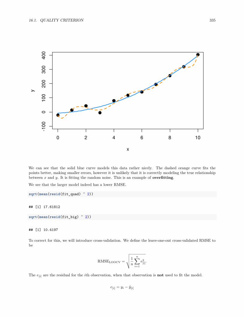
16.1. QUALITY CRITERION 335
0 2 4 6 8 10
-100
010
020
030
040
0
x
y
We can see that the solid blue curve models this data rather nicely. The dashed orange curve fits thepoints better, making smaller errors, however it is unlikely that it is correctly modeling the true relationshipbetween x and y. It is fitting the random noise. This is an example of overfitting.
We see that the larger model indeed has a lower RMSE.
sqrt(mean(resid(fit_quad) ^ 2))
## [1] 17.61812
sqrt(mean(resid(fit_big) ^ 2))
## [1] 10.4197
To correct for this, we will introduce cross-validation. We define the leave-one-out cross-validated RMSE tobe
RMSELOOCV =
√√√√ 1n
n∑i=1
e2[i].
The e[i] are the residual for the ith observation, when that observation is not used to fit the model.
e[i] = yi − y[i]

336 CHAPTER 16. VARIABLE SELECTION AND MODEL BUILDING
That is, the fitted value is calculated as
y[i] = x⊤i β[i]
where β[i] are the estimated coefficients when the ith observation is removed from the dataset.
In general, to perform this calculation, we would be required to fit the model n times, once with eachpossible observation removed. However, for leave-one-out cross-validation and linear models, the equationcan be rewritten as
RMSELOOCV =
√√√√ 1n
n∑i=1
(ei
1 − hi
)2
,
where hi are the leverages and ei are the usual residuals. This is great, because now we can obtain theLOOCV RMSE by fitting only one model! In practice 5 or 10 fold cross-validation are much more popular.For example, in 5-fold cross-validation, the model is fit 5 times, each time leaving out a fifth of the data,then predicting on those values. We’ll leave in-depth examination of cross-validation to a machine learningcourse, and simply use LOOCV here.
Let’s calculate LOOCV RMSE for both models, then discuss why we want to do so. We first write a functionwhich calculates the LOOCV RMSE as defined using the shortcut formula for linear models.
calc_loocv_rmse = function(model) {sqrt(mean((resid(model) / (1 - hatvalues(model))) ^ 2))
}
Then calculate the metric for both models.
calc_loocv_rmse(fit_quad)
## [1] 23.57189
calc_loocv_rmse(fit_big)
## [1] 1334.357
Now we see that the quadratic model has a much smaller LOOCV RMSE, so we would prefer this quadraticmodel. This is because the large model has severely over-fit the data. By leaving a single data point outand fitting the large model, the resulting fit is much different than the fit using all of the data. For example,let’s leave out the third data point and fit both models, then plot the result.
fit_quad_removed = lm(y ~ poly(x, degree = 2), data = poly_data[-3, ])fit_big_removed = lm(y ~ poly(x, degree = 8), data = poly_data[-3, ])
plot(y ~ x, data = poly_data, ylim = c(-100, 400), cex = 2, pch = 20)xplot = seq(0, 10, by = 0.1)lines(xplot, predict(fit_quad_removed, newdata = data.frame(x = xplot)),
col = "dodgerblue", lwd = 2, lty = 1)lines(xplot, predict(fit_big_removed, newdata = data.frame(x = xplot)),
col = "darkorange", lwd = 2, lty = 2)
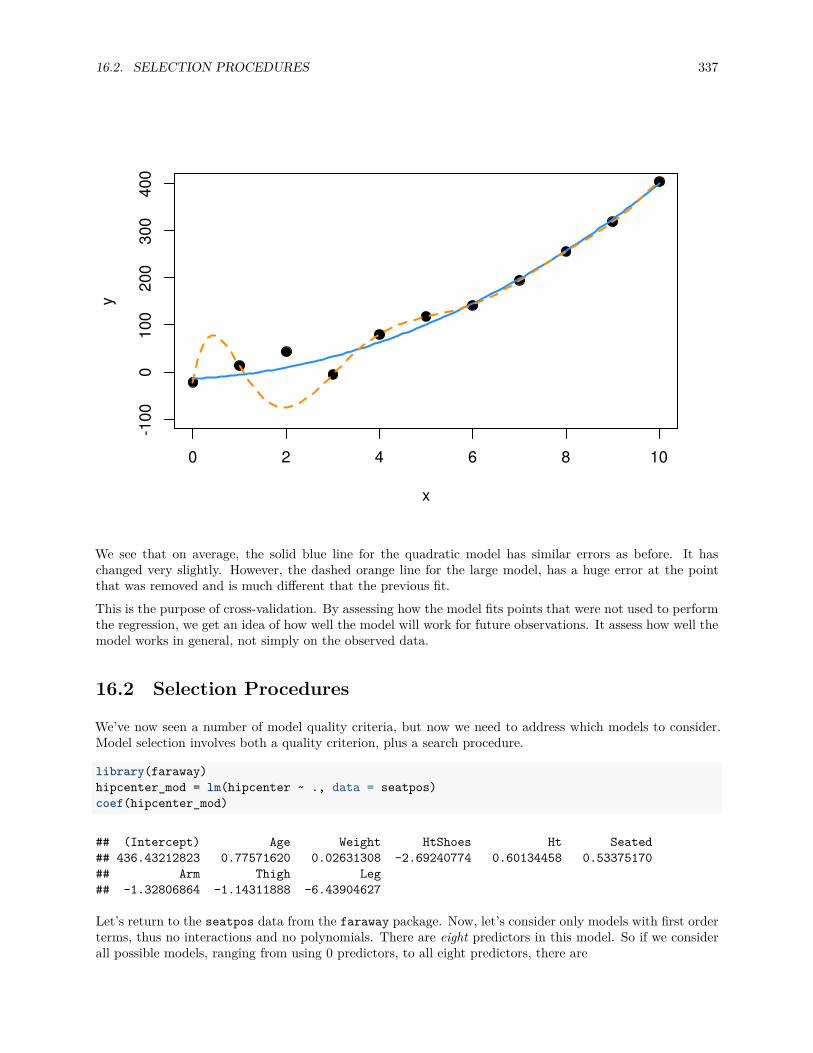
16.2. SELECTION PROCEDURES 337
0 2 4 6 8 10
-100
010
020
030
040
0
x
y
We see that on average, the solid blue line for the quadratic model has similar errors as before. It haschanged very slightly. However, the dashed orange line for the large model, has a huge error at the pointthat was removed and is much different that the previous fit.This is the purpose of cross-validation. By assessing how the model fits points that were not used to performthe regression, we get an idea of how well the model will work for future observations. It assess how well themodel works in general, not simply on the observed data.
16.2 Selection Procedures
We’ve now seen a number of model quality criteria, but now we need to address which models to consider.Model selection involves both a quality criterion, plus a search procedure.
library(faraway)hipcenter_mod = lm(hipcenter ~ ., data = seatpos)coef(hipcenter_mod)
## (Intercept) Age Weight HtShoes Ht Seated## 436.43212823 0.77571620 0.02631308 -2.69240774 0.60134458 0.53375170## Arm Thigh Leg## -1.32806864 -1.14311888 -6.43904627
Let’s return to the seatpos data from the faraway package. Now, let’s consider only models with first orderterms, thus no interactions and no polynomials. There are eight predictors in this model. So if we considerall possible models, ranging from using 0 predictors, to all eight predictors, there are
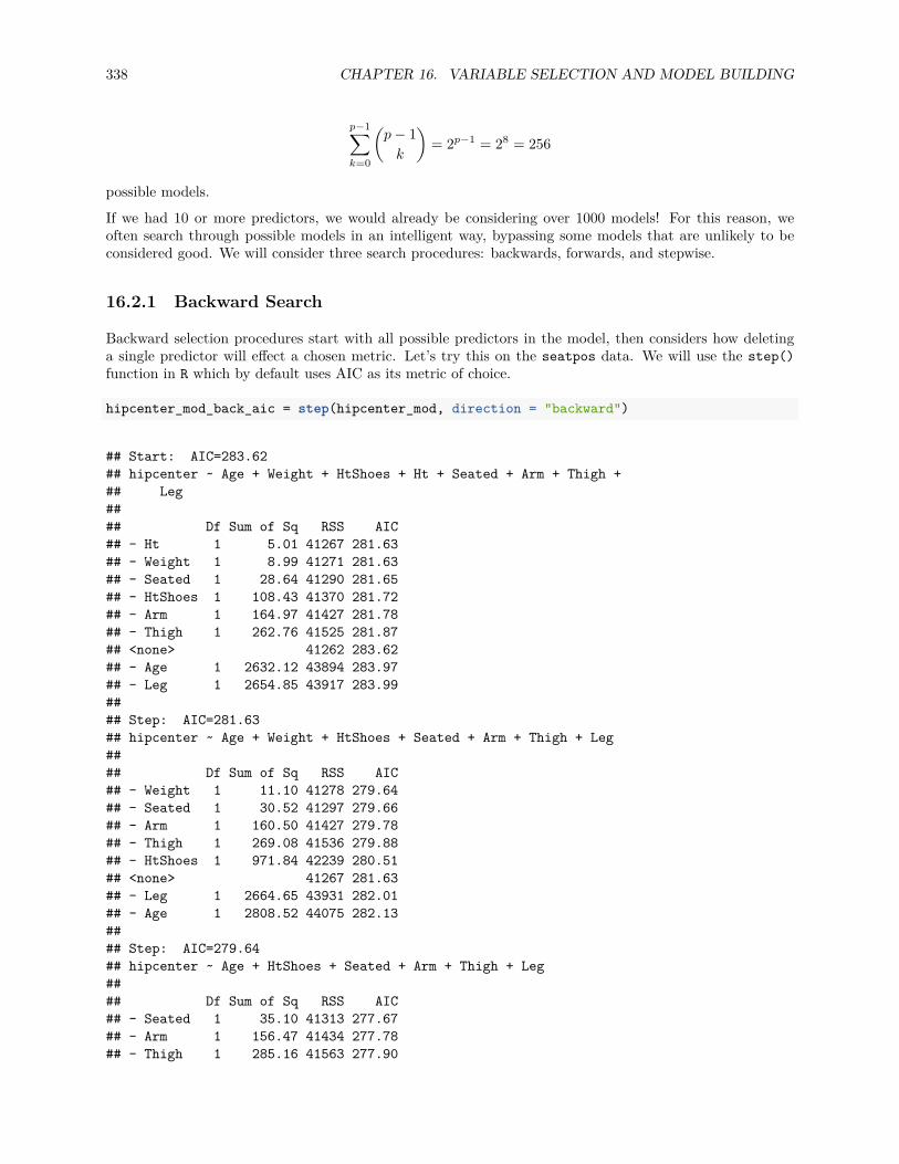
338 CHAPTER 16. VARIABLE SELECTION AND MODEL BUILDING
p−1∑k=0
(p − 1
k
)= 2p−1 = 28 = 256
possible models.
If we had 10 or more predictors, we would already be considering over 1000 models! For this reason, weoften search through possible models in an intelligent way, bypassing some models that are unlikely to beconsidered good. We will consider three search procedures: backwards, forwards, and stepwise.
16.2.1 Backward Search
Backward selection procedures start with all possible predictors in the model, then considers how deletinga single predictor will effect a chosen metric. Let’s try this on the seatpos data. We will use the step()function in R which by default uses AIC as its metric of choice.
hipcenter_mod_back_aic = step(hipcenter_mod, direction = "backward")
## Start: AIC=283.62## hipcenter ~ Age + Weight + HtShoes + Ht + Seated + Arm + Thigh +## Leg#### Df Sum of Sq RSS AIC## - Ht 1 5.01 41267 281.63## - Weight 1 8.99 41271 281.63## - Seated 1 28.64 41290 281.65## - HtShoes 1 108.43 41370 281.72## - Arm 1 164.97 41427 281.78## - Thigh 1 262.76 41525 281.87## <none> 41262 283.62## - Age 1 2632.12 43894 283.97## - Leg 1 2654.85 43917 283.99#### Step: AIC=281.63## hipcenter ~ Age + Weight + HtShoes + Seated + Arm + Thigh + Leg#### Df Sum of Sq RSS AIC## - Weight 1 11.10 41278 279.64## - Seated 1 30.52 41297 279.66## - Arm 1 160.50 41427 279.78## - Thigh 1 269.08 41536 279.88## - HtShoes 1 971.84 42239 280.51## <none> 41267 281.63## - Leg 1 2664.65 43931 282.01## - Age 1 2808.52 44075 282.13#### Step: AIC=279.64## hipcenter ~ Age + HtShoes + Seated + Arm + Thigh + Leg#### Df Sum of Sq RSS AIC## - Seated 1 35.10 41313 277.67## - Arm 1 156.47 41434 277.78## - Thigh 1 285.16 41563 277.90
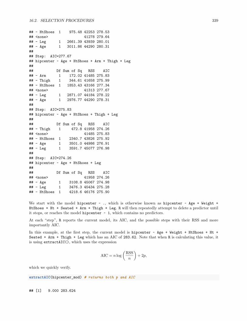
16.2. SELECTION PROCEDURES 339
## - HtShoes 1 975.48 42253 278.53## <none> 41278 279.64## - Leg 1 2661.39 43939 280.01## - Age 1 3011.86 44290 280.31#### Step: AIC=277.67## hipcenter ~ Age + HtShoes + Arm + Thigh + Leg#### Df Sum of Sq RSS AIC## - Arm 1 172.02 41485 275.83## - Thigh 1 344.61 41658 275.99## - HtShoes 1 1853.43 43166 277.34## <none> 41313 277.67## - Leg 1 2871.07 44184 278.22## - Age 1 2976.77 44290 278.31#### Step: AIC=275.83## hipcenter ~ Age + HtShoes + Thigh + Leg#### Df Sum of Sq RSS AIC## - Thigh 1 472.8 41958 274.26## <none> 41485 275.83## - HtShoes 1 2340.7 43826 275.92## - Age 1 3501.0 44986 276.91## - Leg 1 3591.7 45077 276.98#### Step: AIC=274.26## hipcenter ~ Age + HtShoes + Leg#### Df Sum of Sq RSS AIC## <none> 41958 274.26## - Age 1 3108.8 45067 274.98## - Leg 1 3476.3 45434 275.28## - HtShoes 1 4218.6 46176 275.90
We start with the model hipcenter ~ ., which is otherwise known as hipcenter ~ Age + Weight +HtShoes + Ht + Seated + Arm + Thigh + Leg. R will then repeatedly attempt to delete a predictor untilit stops, or reaches the model hipcenter ~ 1, which contains no predictors.
At each “step”, R reports the current model, its AIC, and the possible steps with their RSS and moreimportantly AIC.
In this example, at the first step, the current model is hipcenter ~ Age + Weight + HtShoes + Ht +Seated + Arm + Thigh + Leg which has an AIC of 283.62. Note that when R is calculating this value, itis using extractAIC(), which uses the expression
AIC = n log(
RSSn
)+ 2p,
which we quickly verify.
extractAIC(hipcenter_mod) # returns both p and AIC
## [1] 9.000 283.624

340 CHAPTER 16. VARIABLE SELECTION AND MODEL BUILDING
n = length(resid(hipcenter_mod))(p = length(coef(hipcenter_mod)))
## [1] 9
n * log(mean(resid(hipcenter_mod) ^ 2)) + 2 * p
## [1] 283.624
Returning to the first step, R then gives us a row which shows the effect of deleting each of the currentpredictors. The - signs at the beginning of each row indicates we are considering removing a predictor.There is also a row with <none> which is a row for keeping the current model. Notice that this row has thesmallest RSS, as it is the largest model.
We see that every row above <none> has a smaller AIC than the row for <none> with the one at the top, Ht,giving the lowest AIC. Thus we remove Ht from the model, and continue the process.
Notice, in the second step, we start with the model hipcenter ~ Age + Weight + HtShoes + Seated +Arm + Thigh + Leg and the variable Ht is no longer considered.
We continue the process until we reach the model hipcenter ~ Age + HtShoes + Leg. At this step, therow for <none> tops the list, as removing any additional variable will not improve the AIC This is the modelwhich is stored in hipcenter_mod_back_aic.
coef(hipcenter_mod_back_aic)
## (Intercept) Age HtShoes Leg## 456.2136538 0.5998327 -2.3022555 -6.8297461
We could also search through the possible models in a backwards fashion using BIC. To do so, we again usethe step() function, but now specify k = log(n), where n stores the number of observations in the data.
n = length(resid(hipcenter_mod))hipcenter_mod_back_bic = step(hipcenter_mod, direction = "backward", k = log(n))
## Start: AIC=298.36## hipcenter ~ Age + Weight + HtShoes + Ht + Seated + Arm + Thigh +## Leg#### Df Sum of Sq RSS AIC## - Ht 1 5.01 41267 294.73## - Weight 1 8.99 41271 294.73## - Seated 1 28.64 41290 294.75## - HtShoes 1 108.43 41370 294.82## - Arm 1 164.97 41427 294.88## - Thigh 1 262.76 41525 294.97## - Age 1 2632.12 43894 297.07## - Leg 1 2654.85 43917 297.09## <none> 41262 298.36#### Step: AIC=294.73## hipcenter ~ Age + Weight + HtShoes + Seated + Arm + Thigh + Leg
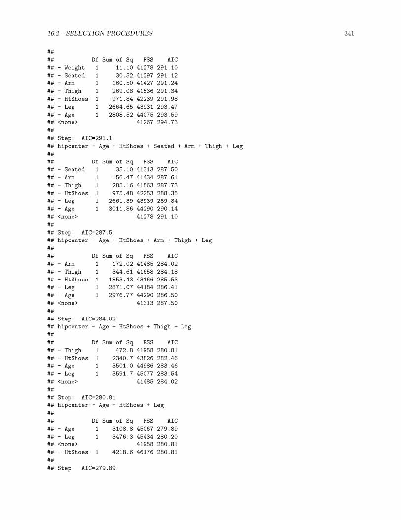
16.2. SELECTION PROCEDURES 341
#### Df Sum of Sq RSS AIC## - Weight 1 11.10 41278 291.10## - Seated 1 30.52 41297 291.12## - Arm 1 160.50 41427 291.24## - Thigh 1 269.08 41536 291.34## - HtShoes 1 971.84 42239 291.98## - Leg 1 2664.65 43931 293.47## - Age 1 2808.52 44075 293.59## <none> 41267 294.73#### Step: AIC=291.1## hipcenter ~ Age + HtShoes + Seated + Arm + Thigh + Leg#### Df Sum of Sq RSS AIC## - Seated 1 35.10 41313 287.50## - Arm 1 156.47 41434 287.61## - Thigh 1 285.16 41563 287.73## - HtShoes 1 975.48 42253 288.35## - Leg 1 2661.39 43939 289.84## - Age 1 3011.86 44290 290.14## <none> 41278 291.10#### Step: AIC=287.5## hipcenter ~ Age + HtShoes + Arm + Thigh + Leg#### Df Sum of Sq RSS AIC## - Arm 1 172.02 41485 284.02## - Thigh 1 344.61 41658 284.18## - HtShoes 1 1853.43 43166 285.53## - Leg 1 2871.07 44184 286.41## - Age 1 2976.77 44290 286.50## <none> 41313 287.50#### Step: AIC=284.02## hipcenter ~ Age + HtShoes + Thigh + Leg#### Df Sum of Sq RSS AIC## - Thigh 1 472.8 41958 280.81## - HtShoes 1 2340.7 43826 282.46## - Age 1 3501.0 44986 283.46## - Leg 1 3591.7 45077 283.54## <none> 41485 284.02#### Step: AIC=280.81## hipcenter ~ Age + HtShoes + Leg#### Df Sum of Sq RSS AIC## - Age 1 3108.8 45067 279.89## - Leg 1 3476.3 45434 280.20## <none> 41958 280.81## - HtShoes 1 4218.6 46176 280.81#### Step: AIC=279.89

342 CHAPTER 16. VARIABLE SELECTION AND MODEL BUILDING
## hipcenter ~ HtShoes + Leg#### Df Sum of Sq RSS AIC## - Leg 1 3038.8 48105 278.73## <none> 45067 279.89## - HtShoes 1 5004.4 50071 280.25#### Step: AIC=278.73## hipcenter ~ HtShoes#### Df Sum of Sq RSS AIC## <none> 48105 278.73## - HtShoes 1 83534 131639 313.35
The procedure is exactly the same, except at each step we look to improve the BIC, which R still labels AICin the output.
The variable hipcenter_mod_back_bic stores the model chosen by this procedure.
coef(hipcenter_mod_back_bic)
## (Intercept) HtShoes## 565.592659 -4.262091
We note that this model is smaller, has fewer predictors, than the model chosen by AIC, which is what wewould expect. Also note that while both models are different, neither uses both Ht and HtShoes which areextremely correlated.
We can use information from the summary() function to compare their Adjusted R2 values. Note that eitherselected model performs better than the original full model.
summary(hipcenter_mod)$adj.r.squared
## [1] 0.6000855
summary(hipcenter_mod_back_aic)$adj.r.squared
## [1] 0.6531427
summary(hipcenter_mod_back_bic)$adj.r.squared
## [1] 0.6244149
We can also calculate the LOOCV RMSE for both selected models, as well as the full model.
calc_loocv_rmse(hipcenter_mod)
## [1] 44.44564

16.2. SELECTION PROCEDURES 343
calc_loocv_rmse(hipcenter_mod_back_aic)
## [1] 37.58473
calc_loocv_rmse(hipcenter_mod_back_bic)
## [1] 37.40564
We see that we would prefer the model chosen via BIC if using LOOCV RMSE as our metric.
16.2.2 Forward Search
Forward selection is the exact opposite of backwards selection. Here we tell R to start with a model using nopredictors, that is hipcenter ~ 1, then at each step R will attempt to add a predictor until it finds a goodmodel or reaches hipcenter ~ Age + Weight + HtShoes + Ht + Seated + Arm + Thigh + Leg.
hipcenter_mod_start = lm(hipcenter ~ 1, data = seatpos)hipcenter_mod_forw_aic = step(hipcenter_mod_start,scope = hipcenter ~ Age + Weight + HtShoes + Ht + Seated + Arm + Thigh + Leg,direction = "forward")
## Start: AIC=311.71## hipcenter ~ 1#### Df Sum of Sq RSS AIC## + Ht 1 84023 47616 275.07## + HtShoes 1 83534 48105 275.45## + Leg 1 81568 50071 276.98## + Seated 1 70392 61247 284.63## + Weight 1 53975 77664 293.66## + Thigh 1 46010 85629 297.37## + Arm 1 45065 86574 297.78## <none> 131639 311.71## + Age 1 5541 126098 312.07#### Step: AIC=275.07## hipcenter ~ Ht#### Df Sum of Sq RSS AIC## + Leg 1 2781.10 44835 274.78## <none> 47616 275.07## + Age 1 2353.51 45262 275.14## + Weight 1 195.86 47420 276.91## + Seated 1 101.56 47514 276.99## + Arm 1 75.78 47540 277.01## + HtShoes 1 25.76 47590 277.05## + Thigh 1 4.63 47611 277.06#### Step: AIC=274.78## hipcenter ~ Ht + Leg

344 CHAPTER 16. VARIABLE SELECTION AND MODEL BUILDING
#### Df Sum of Sq RSS AIC## + Age 1 2896.60 41938 274.24## <none> 44835 274.78## + Arm 1 522.72 44312 276.33## + Weight 1 445.10 44390 276.40## + HtShoes 1 34.11 44801 276.75## + Thigh 1 32.96 44802 276.75## + Seated 1 1.12 44834 276.78#### Step: AIC=274.24## hipcenter ~ Ht + Leg + Age#### Df Sum of Sq RSS AIC## <none> 41938 274.24## + Thigh 1 372.71 41565 275.90## + Arm 1 257.09 41681 276.01## + Seated 1 121.26 41817 276.13## + Weight 1 46.83 41891 276.20## + HtShoes 1 13.38 41925 276.23
Again, by default R uses AIC as its quality metric when using the step() function. Also note that now therows begin with a + which indicates addition of predictors to the current model from any step.
hipcenter_mod_forw_bic = step(hipcenter_mod_start,scope = hipcenter ~ Age + Weight + HtShoes + Ht + Seated + Arm + Thigh + Leg,direction = "forward", k = log(n))
## Start: AIC=313.35## hipcenter ~ 1#### Df Sum of Sq RSS AIC## + Ht 1 84023 47616 278.34## + HtShoes 1 83534 48105 278.73## + Leg 1 81568 50071 280.25## + Seated 1 70392 61247 287.91## + Weight 1 53975 77664 296.93## + Thigh 1 46010 85629 300.64## + Arm 1 45065 86574 301.06## <none> 131639 313.35## + Age 1 5541 126098 315.35#### Step: AIC=278.34## hipcenter ~ Ht#### Df Sum of Sq RSS AIC## <none> 47616 278.34## + Leg 1 2781.10 44835 279.69## + Age 1 2353.51 45262 280.05## + Weight 1 195.86 47420 281.82## + Seated 1 101.56 47514 281.90## + Arm 1 75.78 47540 281.92

16.2. SELECTION PROCEDURES 345
## + HtShoes 1 25.76 47590 281.96## + Thigh 1 4.63 47611 281.98
We can make the same modification as last time to instead use BIC with forward selection.
summary(hipcenter_mod)$adj.r.squared
## [1] 0.6000855
summary(hipcenter_mod_forw_aic)$adj.r.squared
## [1] 0.6533055
summary(hipcenter_mod_forw_bic)$adj.r.squared
## [1] 0.6282374
We can compare the two selected models’ Adjusted R2 as well as their LOOCV RMSE The results are verysimilar to those using backwards selection, although the models are not exactly the same.
calc_loocv_rmse(hipcenter_mod)
## [1] 44.44564
calc_loocv_rmse(hipcenter_mod_forw_aic)
## [1] 37.62516
calc_loocv_rmse(hipcenter_mod_forw_bic)
## [1] 37.2511
16.2.3 Stepwise Search
Stepwise search checks going both backwards and forwards at every step. It considers the addition of anyvariable not currently in the model, as well as the removal of any variable currently in the model.
Here we perform stepwise search using AIC as our metric. We start with the model hipcenter ~ 1 andsearch up to hipcenter ~ Age + Weight + HtShoes + Ht + Seated + Arm + Thigh + Leg. Notice thatat many of the steps, some row begin with -, while others begin with +.
hipcenter_mod_both_aic = step(hipcenter_mod_start,scope = hipcenter ~ Age + Weight + HtShoes + Ht + Seated + Arm + Thigh + Leg,direction = "both")
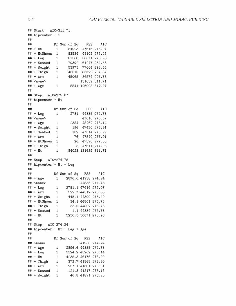
346 CHAPTER 16. VARIABLE SELECTION AND MODEL BUILDING
## Start: AIC=311.71## hipcenter ~ 1#### Df Sum of Sq RSS AIC## + Ht 1 84023 47616 275.07## + HtShoes 1 83534 48105 275.45## + Leg 1 81568 50071 276.98## + Seated 1 70392 61247 284.63## + Weight 1 53975 77664 293.66## + Thigh 1 46010 85629 297.37## + Arm 1 45065 86574 297.78## <none> 131639 311.71## + Age 1 5541 126098 312.07#### Step: AIC=275.07## hipcenter ~ Ht#### Df Sum of Sq RSS AIC## + Leg 1 2781 44835 274.78## <none> 47616 275.07## + Age 1 2354 45262 275.14## + Weight 1 196 47420 276.91## + Seated 1 102 47514 276.99## + Arm 1 76 47540 277.01## + HtShoes 1 26 47590 277.05## + Thigh 1 5 47611 277.06## - Ht 1 84023 131639 311.71#### Step: AIC=274.78## hipcenter ~ Ht + Leg#### Df Sum of Sq RSS AIC## + Age 1 2896.6 41938 274.24## <none> 44835 274.78## - Leg 1 2781.1 47616 275.07## + Arm 1 522.7 44312 276.33## + Weight 1 445.1 44390 276.40## + HtShoes 1 34.1 44801 276.75## + Thigh 1 33.0 44802 276.75## + Seated 1 1.1 44834 276.78## - Ht 1 5236.3 50071 276.98#### Step: AIC=274.24## hipcenter ~ Ht + Leg + Age#### Df Sum of Sq RSS AIC## <none> 41938 274.24## - Age 1 2896.6 44835 274.78## - Leg 1 3324.2 45262 275.14## - Ht 1 4238.3 46176 275.90## + Thigh 1 372.7 41565 275.90## + Arm 1 257.1 41681 276.01## + Seated 1 121.3 41817 276.13## + Weight 1 46.8 41891 276.20

16.2. SELECTION PROCEDURES 347
## + HtShoes 1 13.4 41925 276.23
We could again instead use BIC as our metric.
hipcenter_mod_both_bic = step(hipcenter_mod_start,scope = hipcenter ~ Age + Weight + HtShoes + Ht + Seated + Arm + Thigh + Leg,direction = "both", k = log(n))
## Start: AIC=313.35## hipcenter ~ 1#### Df Sum of Sq RSS AIC## + Ht 1 84023 47616 278.34## + HtShoes 1 83534 48105 278.73## + Leg 1 81568 50071 280.25## + Seated 1 70392 61247 287.91## + Weight 1 53975 77664 296.93## + Thigh 1 46010 85629 300.64## + Arm 1 45065 86574 301.06## <none> 131639 313.35## + Age 1 5541 126098 315.35#### Step: AIC=278.34## hipcenter ~ Ht#### Df Sum of Sq RSS AIC## <none> 47616 278.34## + Leg 1 2781 44835 279.69## + Age 1 2354 45262 280.05## + Weight 1 196 47420 281.82## + Seated 1 102 47514 281.90## + Arm 1 76 47540 281.92## + HtShoes 1 26 47590 281.96## + Thigh 1 5 47611 281.98## - Ht 1 84023 131639 313.35
Adjusted R2 and LOOCV RMSE comparisons are similar to backwards and forwards, which is not at allsurprising, as some of the models selected are the same as before.
summary(hipcenter_mod)$adj.r.squared
## [1] 0.6000855
summary(hipcenter_mod_both_aic)$adj.r.squared
## [1] 0.6533055
summary(hipcenter_mod_both_bic)$adj.r.squared
## [1] 0.6282374

348 CHAPTER 16. VARIABLE SELECTION AND MODEL BUILDING
calc_loocv_rmse(hipcenter_mod)
## [1] 44.44564
calc_loocv_rmse(hipcenter_mod_both_aic)
## [1] 37.62516
calc_loocv_rmse(hipcenter_mod_both_bic)
## [1] 37.2511
16.2.4 Exhaustive Search
Backward, forward, and stepwise search are all useful, but do have an obvious issue. By not checking everypossible model, sometimes they will miss the best possible model. With an extremely large number ofpredictors, sometimes this is necessary since checking every possible model would be rather time consuming,even with current computers.
However, with a reasonably sized dataset, it isn’t too difficult to check all possible models. To do so, we willuse the regsubsets() function in the R package leaps.
library(leaps)all_hipcenter_mod = summary(regsubsets(hipcenter ~ ., data = seatpos))
A few points about this line of code. First, note that we immediately use summary() and store those results.That is simply the intended use of regsubsets(). Second, inside of regsubsets() we specify the modelhipcenter ~ .. This will be the largest model considered, that is the model using all first-order predictors,and R will check all possible subsets.
We’ll now look at the information stored in all_hipcenter_mod.
all_hipcenter_mod$which
## (Intercept) Age Weight HtShoes Ht Seated Arm Thigh Leg## 1 TRUE FALSE FALSE FALSE TRUE FALSE FALSE FALSE FALSE## 2 TRUE FALSE FALSE FALSE TRUE FALSE FALSE FALSE TRUE## 3 TRUE TRUE FALSE FALSE TRUE FALSE FALSE FALSE TRUE## 4 TRUE TRUE FALSE TRUE FALSE FALSE FALSE TRUE TRUE## 5 TRUE TRUE FALSE TRUE FALSE FALSE TRUE TRUE TRUE## 6 TRUE TRUE FALSE TRUE FALSE TRUE TRUE TRUE TRUE## 7 TRUE TRUE TRUE TRUE FALSE TRUE TRUE TRUE TRUE## 8 TRUE TRUE TRUE TRUE TRUE TRUE TRUE TRUE TRUE
Using $which gives us the best model, according to RSS, for a model of each possible size, in this caseranging from one to eight predictors. For example the best model with four predictors (p = 5) would useAge, HtShoes, Thigh, and Leg.
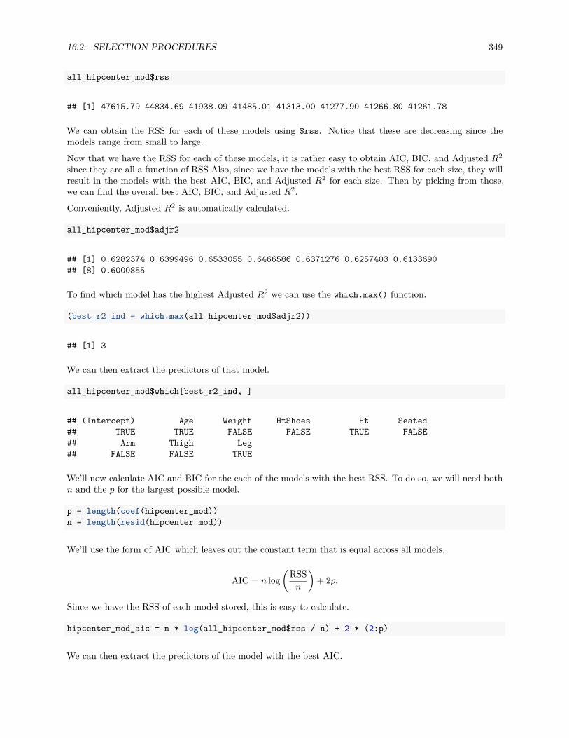
16.2. SELECTION PROCEDURES 349
all_hipcenter_mod$rss
## [1] 47615.79 44834.69 41938.09 41485.01 41313.00 41277.90 41266.80 41261.78
We can obtain the RSS for each of these models using $rss. Notice that these are decreasing since themodels range from small to large.
Now that we have the RSS for each of these models, it is rather easy to obtain AIC, BIC, and Adjusted R2
since they are all a function of RSS Also, since we have the models with the best RSS for each size, they willresult in the models with the best AIC, BIC, and Adjusted R2 for each size. Then by picking from those,we can find the overall best AIC, BIC, and Adjusted R2.
Conveniently, Adjusted R2 is automatically calculated.
all_hipcenter_mod$adjr2
## [1] 0.6282374 0.6399496 0.6533055 0.6466586 0.6371276 0.6257403 0.6133690## [8] 0.6000855
To find which model has the highest Adjusted R2 we can use the which.max() function.
(best_r2_ind = which.max(all_hipcenter_mod$adjr2))
## [1] 3
We can then extract the predictors of that model.
all_hipcenter_mod$which[best_r2_ind, ]
## (Intercept) Age Weight HtShoes Ht Seated## TRUE TRUE FALSE FALSE TRUE FALSE## Arm Thigh Leg## FALSE FALSE TRUE
We’ll now calculate AIC and BIC for the each of the models with the best RSS. To do so, we will need bothn and the p for the largest possible model.
p = length(coef(hipcenter_mod))n = length(resid(hipcenter_mod))
We’ll use the form of AIC which leaves out the constant term that is equal across all models.
AIC = n log(
RSSn
)+ 2p.
Since we have the RSS of each model stored, this is easy to calculate.
hipcenter_mod_aic = n * log(all_hipcenter_mod$rss / n) + 2 * (2:p)
We can then extract the predictors of the model with the best AIC.

350 CHAPTER 16. VARIABLE SELECTION AND MODEL BUILDING
best_aic_ind = which.min(hipcenter_mod_aic)all_hipcenter_mod$which[best_aic_ind,]
## (Intercept) Age Weight HtShoes Ht Seated## TRUE TRUE FALSE FALSE TRUE FALSE## Arm Thigh Leg## FALSE FALSE TRUE
Let’s fit this model so we can compare to our previously chosen models using AIC and search procedures.
hipcenter_mod_best_aic = lm(hipcenter ~ Age + Ht + Leg, data = seatpos)
The extractAIC() function will calculate the AIC defined above for a fitted model.
extractAIC(hipcenter_mod_best_aic)
## [1] 4.0000 274.2418
extractAIC(hipcenter_mod_back_aic)
## [1] 4.0000 274.2597
extractAIC(hipcenter_mod_forw_aic)
## [1] 4.0000 274.2418
extractAIC(hipcenter_mod_both_aic)
## [1] 4.0000 274.2418
We see that two of the models chosen by search procedures have the best possible AIC, as they are the samemodel. This is however never guaranteed. We see that the model chosen using backwards selection does notachieve the smallest possible AIC.
plot(hipcenter_mod_aic ~ I(2:p), ylab = "AIC", xlab = "p, number of parameters",pch = 20, col = "dodgerblue", type = "b", cex = 2,main = "AIC vs Model Complexity")
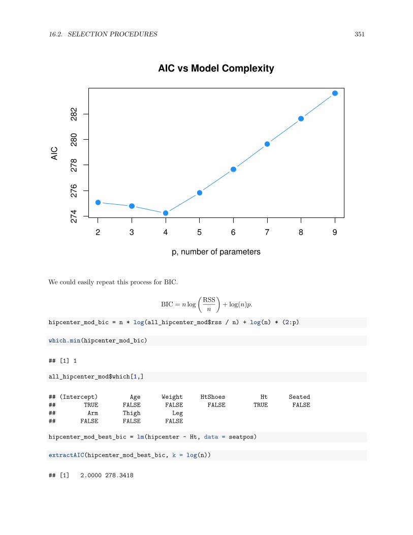
16.2. SELECTION PROCEDURES 351
2 3 4 5 6 7 8 9
274
276
278
280
282
AIC vs Model Complexity
p, number of parameters
AIC
We could easily repeat this process for BIC.
BIC = n log(
RSSn
)+ log(n)p.
hipcenter_mod_bic = n * log(all_hipcenter_mod$rss / n) + log(n) * (2:p)
which.min(hipcenter_mod_bic)
## [1] 1
all_hipcenter_mod$which[1,]
## (Intercept) Age Weight HtShoes Ht Seated## TRUE FALSE FALSE FALSE TRUE FALSE## Arm Thigh Leg## FALSE FALSE FALSE
hipcenter_mod_best_bic = lm(hipcenter ~ Ht, data = seatpos)
extractAIC(hipcenter_mod_best_bic, k = log(n))
## [1] 2.0000 278.3418

352 CHAPTER 16. VARIABLE SELECTION AND MODEL BUILDING
extractAIC(hipcenter_mod_back_bic, k = log(n))
## [1] 2.0000 278.7306
extractAIC(hipcenter_mod_forw_bic, k = log(n))
## [1] 2.0000 278.3418
extractAIC(hipcenter_mod_both_bic, k = log(n))
## [1] 2.0000 278.3418
16.3 Higher Order Terms
So far we have only allowed first-order terms in our models. Let’s return to the autompg dataset to explorehigher-order terms.
autompg = read.table("http://archive.ics.uci.edu/ml/machine-learning-databases/auto-mpg/auto-mpg.data",quote = "\"",comment.char = "",stringsAsFactors = FALSE)
colnames(autompg) = c("mpg", "cyl", "disp", "hp", "wt", "acc","year", "origin", "name")
autompg = subset(autompg, autompg$hp != "?")autompg = subset(autompg, autompg$name != "plymouth reliant")rownames(autompg) = paste(autompg$cyl, "cylinder", autompg$year, autompg$name)autompg$hp = as.numeric(autompg$hp)autompg$domestic = as.numeric(autompg$origin == 1)autompg = autompg[autompg$cyl != 5,]autompg = autompg[autompg$cyl != 3,]autompg$cyl = as.factor(autompg$cyl)autompg$domestic = as.factor(autompg$domestic)autompg = subset(autompg, select = c("mpg", "cyl", "disp", "hp",
"wt", "acc", "year", "domestic"))
str(autompg)
## 'data.frame': 383 obs. of 8 variables:## $ mpg : num 18 15 18 16 17 15 14 14 14 15 ...## $ cyl : Factor w/ 3 levels "4","6","8": 3 3 3 3 3 3 3 3 3 3 ...## $ disp : num 307 350 318 304 302 429 454 440 455 390 ...## $ hp : num 130 165 150 150 140 198 220 215 225 190 ...## $ wt : num 3504 3693 3436 3433 3449 ...## $ acc : num 12 11.5 11 12 10.5 10 9 8.5 10 8.5 ...## $ year : int 70 70 70 70 70 70 70 70 70 70 ...## $ domestic: Factor w/ 2 levels "0","1": 2 2 2 2 2 2 2 2 2 2 ...

16.3. HIGHER ORDER TERMS 353
Recall that we have two factor variables, cyl and domestic. The cyl variable has three levels, while thedomestic variable has only two. Thus the cyl variable will be coded using two dummy variables, while thedomestic variable will only need one. We will pay attention to this later.
pairs(autompg, col = "dodgerblue")
mpg
1.0 2.0 3.0 50 150 10 20 1.0 1.4 1.8
1030
1.0
2.0
3.0
cyl
disp
100
300
5015
0 hp
wt
1500
3500
1020
acc
year70
7478
82
10 30
1.0
1.4
1.8
100 300 1500 3500 70 74 78 82
domestic
We’ll use the pairs() plot to determine which variables may benefit from a quadratic relationship with theresponse. We’ll also consider all possible two-way interactions. We won’t consider any three-order or higher.For example, we won’t consider the interaction between first-order terms and the added quadratic terms.So now, we’ll fit this rather large model. We’ll use a log-transformed response. Notice that log(mpg) ~ .^ 2 will automatically consider all first-order terms, as well as all two-way interactions. We use I(var_name^ 2) to add quadratic terms for some variables. This generally works better than using poly() whenperforming variable selection.

354 CHAPTER 16. VARIABLE SELECTION AND MODEL BUILDING
autompg_big_mod = lm(log(mpg) ~ . ^ 2 + I(disp ^ 2) + I(hp ^ 2) + I(wt ^ 2) + I(acc ^ 2),data = autompg)
We think it is rather unlikely that we truly need all of these terms. There are quite a few!
length(coef(autompg_big_mod))
## [1] 40
We’ll try backwards search with both AIC and BIC to attempt to find a smaller, more reasonable model.
autompg_mod_back_aic = step(autompg_big_mod, direction = "backward", trace = 0)
Notice that we used trace = 0 in the function call. This suppress the output for each step, and simplystores the chosen model. This is useful, as this code would otherwise create a large amount of output. If wehad viewed the output, which you can try on your own by removing trace = 0, we would see that R onlyconsiders the cyl variable as a single variable, despite the fact that it is coded using two dummy variables.So removing cyl would actually remove two parameters from the resulting model.You should also notice that R respects hierarchy when attempting to remove variables. That is, for example,R will not consider removing hp if hp:disp or I(hp ^ 2) are currently in the model.We also use BIC.
n = length(resid(autompg_big_mod))autompg_mod_back_bic = step(autompg_big_mod, direction = "backward",
k = log(n), trace = 0)
Looking at the coefficients of the two chosen models, we see they are still rather large.
coef(autompg_mod_back_aic)
## (Intercept) cyl6 cyl8 disp## 3.6718839511472 -0.1602563336333 -0.8581644338393 -0.0093719707873## hp wt acc year## 0.0229353409493 -0.0003064496949 -0.1393888479750 -0.0019663606344## domestic1 I(hp^2) cyl6:acc cyl8:acc## 0.9369323953411 -0.0000149766900 0.0072202979695 0.0504191492217## disp:wt disp:year hp:acc hp:year## 0.0000005797816 0.0000949376953 -0.0005062294609 -0.0001838985017## acc:year acc:domestic1 year:domestic1## 0.0023456252781 -0.0237246840975 -0.0073327246317
coef(autompg_mod_back_bic)
## (Intercept) cyl6 cyl8 disp## 4.6578470390516 -0.1086165018406 -0.7611630775038 -0.0016093164199## hp wt acc year## 0.0026212660296 -0.0002635971659 -0.1670601021732 -0.0104564626969## domestic1 cyl6:acc cyl8:acc disp:wt## 0.3341578960873 0.0043154925327 0.0461009496981 0.0000004102804## hp:acc acc:year acc:domestic1## -0.0003386261424 0.0025001372156 -0.0219329407492

16.4. EXPLANATION VERSUS PREDICTION 355
However, they are much smaller than the original full model. Also notice that the resulting models respecthierarchy.
length(coef(autompg_big_mod))
## [1] 40
length(coef(autompg_mod_back_aic))
## [1] 19
length(coef(autompg_mod_back_bic))
## [1] 15
Calculating the LOOCV RMSE for each, we see that the model chosen using BIC performs the best. Thatmeans that it is both the best model for prediction, since it achieves the best LOOCV RMSE, but also thebest model for explanation, as it is also the smallest.
calc_loocv_rmse(autompg_big_mod)
## [1] 0.1112024
calc_loocv_rmse(autompg_mod_back_aic)
## [1] 0.1032888
calc_loocv_rmse(autompg_mod_back_bic)
## [1] 0.103134
16.4 Explanation versus Prediction
Throughout this chapter, we have attempted to find reasonably “small” models, which are good at explain-ing the relationship between the response and the predictors, that also have small errors which are thusgood for making predictions.
We’ll further discuss the model autompg_mod_back_bic to better explain the difference between using modelsfor explaining and predicting. This is the model fit to the autompg data that was chosen using BackwardsSearch and BIC, which obtained the lowest LOOCV RMSE of the models we considered.
autompg_mod_back_bic
#### Call:## lm(formula = log(mpg) ~ cyl + disp + hp + wt + acc + year + domestic +## cyl:acc + disp:wt + hp:acc + acc:year + acc:domestic, data = autompg)##

356 CHAPTER 16. VARIABLE SELECTION AND MODEL BUILDING
## Coefficients:## (Intercept) cyl6 cyl8 disp hp## 4.6578470391 -0.1086165018 -0.7611630775 -0.0016093164 0.0026212660## wt acc year domestic1 cyl6:acc## -0.0002635972 -0.1670601022 -0.0104564627 0.3341578961 0.0043154925## cyl8:acc disp:wt hp:acc acc:year acc:domestic1## 0.0461009497 0.0000004103 -0.0003386261 0.0025001372 -0.0219329407
Notice this is a somewhat “large” model, which uses 15 parameters, including several interaction terms. Dowe care that this is a “large” model? The answer is, it depends.
16.4.1 Explanation
Suppose we would like to use this model for explanation. Perhaps we are a car manufacturer trying to engineera fuel efficient vehicle. If this is the case, we are interested in both what predictor variables are useful forexplaining the car’s fuel efficiency, as well as how those variables effect fuel efficiency. By understanding thisrelationship, we can use this knowledge to our advantage when designing a car.
To explain a relationship, we are interested in keeping models as small as possible, since smaller modelsare easy to interpret. The fewer predictors the less considerations we need to make in our design process.Also the fewer interactions and polynomial terms, the easier it is to interpret any one parameter, since theparameter interpretations are conditional on which parameters are in the model.
Note that linear models are rather interpretable to begin with. Later in your data analysis careers, you willsee more complicated models that may fit data better, but are much harder, if not impossible to interpret.These models aren’t very useful for explaining a relationship.
To find small and interpretable models, we would use selection criterion that explicitly penalize larger models,such as AIC and BIC. In this case we still obtained a somewhat large model, but much smaller than themodel we used to start the selection process.
16.4.1.1 Correlation and Causation
A word of caution when using a model to explain a relationship. There are two terms often used to describea relationship between two variables: causation and correlation. Correlation is often also referred to asassociation.
Just because two variable are correlated does not necessarily mean that one causes the other. For example,considering modeling mpg as only a function of hp.
plot(mpg ~ hp, data = autompg, col = "dodgerblue", pch = 20, cex = 1.5)
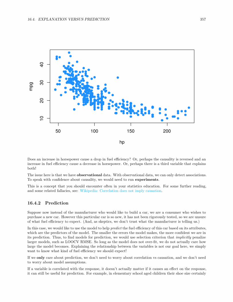
16.4. EXPLANATION VERSUS PREDICTION 357
50 100 150 200
1020
3040
hp
mpg
Does an increase in horsepower cause a drop in fuel efficiency? Or, perhaps the causality is reversed and anincrease in fuel efficiency cause a decrease in horsepower. Or, perhaps there is a third variable that explainsboth!The issue here is that we have observational data. With observational data, we can only detect associations.To speak with confidence about causality, we would need to run experiments.This is a concept that you should encounter often in your statistics education. For some further reading,and some related fallacies, see: Wikipedia: Correlation does not imply causation.
16.4.2 Prediction
Suppose now instead of the manufacturer who would like to build a car, we are a consumer who wishes topurchase a new car. However this particular car is so new, it has not been rigorously tested, so we are unsureof what fuel efficiency to expect. (And, as skeptics, we don’t trust what the manufacturer is telling us.)In this case, we would like to use the model to help predict the fuel efficiency of this car based on its attributes,which are the predictors of the model. The smaller the errors the model makes, the more confident we are inits prediction. Thus, to find models for prediction, we would use selection criterion that implicitly penalizelarger models, such as LOOCV RMSE. So long as the model does not over-fit, we do not actually care howlarge the model becomes. Explaining the relationship between the variables is not our goal here, we simplywant to know what kind of fuel efficiency we should expect!If we only care about prediction, we don’t need to worry about correlation vs causation, and we don’t needto worry about model assumptions.If a variable is correlated with the response, it doesn’t actually matter if it causes an effect on the response,it can still be useful for prediction. For example, in elementary school aged children their shoe size certainly

358 CHAPTER 16. VARIABLE SELECTION AND MODEL BUILDING
doesn’t cause them to read at a higher level, however we could very easily use shoe size to make a predictionabout a child’s reading ability. The larger their shoe size, the better they read. There’s a lurking variablehere though, their age! (Don’t send your kids to school with size 14 shoes, it won’t make them read better!)
We also don’t care about model assumptions. Least squares is least squares. For a specified model, it willfind the values of the parameters which will minimize the squared error loss. Your results might be largelyuninterpretable and useless for inference, but for prediction none of that matters.
Chapter 17
Logistic Regression
Note to current readers: This chapter is slightly less tested than previous chapters. Please do not hesitateto report any errors, or suggest sections that need better explanation! Also, as a result, this material is morelikely to receive edits.
After reading this chapter you will be able to:
• Understand how generalized linear models are a generalization of ordinary linear models.• Use logistic regression to model a binary response.• Apply concepts learned for ordinary linear models to logistic regression.• Use logistic regression to perform classification.
So far we have only considered models for numeric response variables. What about response variables thatonly take integer values? What about a response variable that is categorical? Can we use linear models inthese situations? Yes! The model that we have been using, which we will call ordinary linear regression, isactually a specific case of the more general, generalized linear model. (Aren’t statisticians great at namingthings?)
17.1 Generalized Linear Models
So far, we’ve had response variables that, conditioned on the predictors, were modeled using a normaldistribution with a mean that is some linear combination of the predictors. This linear combination is whatmade a linear model “linear.”
Y | X = x ∼ N(β0 + β1x1 + . . . + βp−1xp−1, σ2)
Now we’ll allow for two modifications of this situation, which will let us use linear models in many moresituations. Instead of using a normal distribution for the response, we’ll allow for other distributions. Also,instead of the mean being a linear combination of the predictors, it can be some function of a linear combi-nation of the predictors.
In general, a generalized linear model has three parts:
• A distribution of the response conditioned on the predictors. (Technically this distribution needs tobe from the exponential family of distributions.)
• A linear combination of the p − 1 predictors, β0 + β1x1 + β2x2 + . . . + βp−1xp−1, which we write asη(x). That is,
359
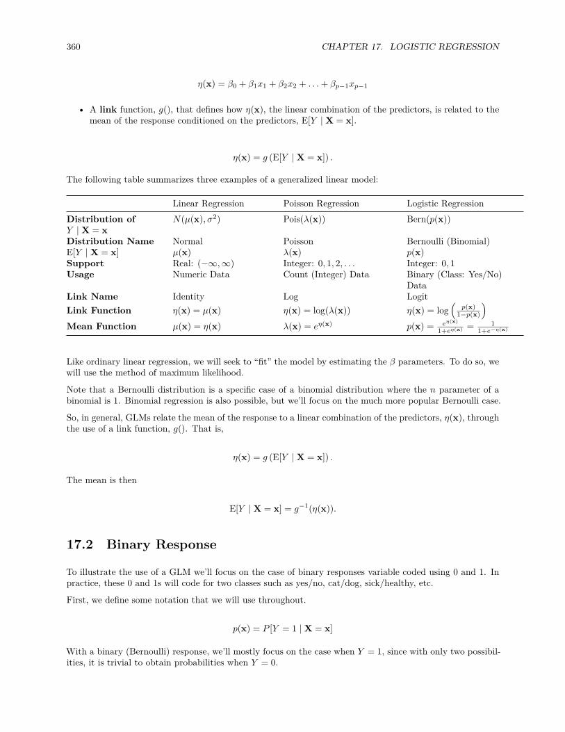
360 CHAPTER 17. LOGISTIC REGRESSION
η(x) = β0 + β1x1 + β2x2 + . . . + βp−1xp−1
• A link function, g(), that defines how η(x), the linear combination of the predictors, is related to themean of the response conditioned on the predictors, E[Y | X = x].
η(x) = g (E[Y | X = x]) .
The following table summarizes three examples of a generalized linear model:
Linear Regression Poisson Regression Logistic RegressionDistribution ofY | X = x
N(µ(x), σ2) Pois(λ(x)) Bern(p(x))
Distribution Name Normal Poisson Bernoulli (Binomial)E[Y | X = x] µ(x) λ(x) p(x)Support Real: (−∞, ∞) Integer: 0, 1, 2, . . . Integer: 0, 1Usage Numeric Data Count (Integer) Data Binary (Class: Yes/No)
DataLink Name Identity Log LogitLink Function η(x) = µ(x) η(x) = log(λ(x)) η(x) = log
(p(x)
1−p(x)
)Mean Function µ(x) = η(x) λ(x) = eη(x) p(x) = eη(x)
1+eη(x) = 11+e−η(x)
Like ordinary linear regression, we will seek to “fit” the model by estimating the β parameters. To do so, wewill use the method of maximum likelihood.
Note that a Bernoulli distribution is a specific case of a binomial distribution where the n parameter of abinomial is 1. Binomial regression is also possible, but we’ll focus on the much more popular Bernoulli case.
So, in general, GLMs relate the mean of the response to a linear combination of the predictors, η(x), throughthe use of a link function, g(). That is,
η(x) = g (E[Y | X = x]) .
The mean is then
E[Y | X = x] = g−1(η(x)).
17.2 Binary Response
To illustrate the use of a GLM we’ll focus on the case of binary responses variable coded using 0 and 1. Inpractice, these 0 and 1s will code for two classes such as yes/no, cat/dog, sick/healthy, etc.
First, we define some notation that we will use throughout.
p(x) = P [Y = 1 | X = x]
With a binary (Bernoulli) response, we’ll mostly focus on the case when Y = 1, since with only two possibil-ities, it is trivial to obtain probabilities when Y = 0.
17.2. BINARY RESPONSE 361
P [Y = 0 | X = x] + P [Y = 1 | X = x] = 1
P [Y = 0 | X = x] = 1 − p(x)
We now define the logistic regression model.
log(
p(x)1 − p(x)
)= β0 + β1x1 + . . . + βp−1xp−1
Immediately we notice some similarities to ordinary linear regression, in particular, the right hand side.This is our usual linear combination of the predictors. We have our usual p − 1 predictors for a total of p βparameters. (Note, many more machine learning focused texts will use p as the number of parameters. Thisis an arbitrary choice, but you should be aware of it.)
The right hand side is called the log odds, which is the log of the odds. The odds are the probability for apositive event (Y = 1) divided by the probability of a negative event (Y = 0). So when the odds are 1, thetwo events have equal probability. Odds greater than 1 favor a positive event. The opposite is true whenthe odds are less than 1.
p(x)1 − p(x)
= P [Y = 1 | X = x]P [Y = 0 | X = x]
Essentially, the log odds are the logit transform applied to p(x).
logit(x) = log(
x
1 − x
)It will also be useful to define the inverse logit, otherwise known as the “logistic” or sigmoid function.
logit−1(x) = ex
1 + ex= 1
1 + e−x
Note that for x ∈ (−∞, ∞)), this function outputs values between 0 and 1.
Students often ask, where is the error term? The answer is that its something that is specific to the normalmodel. First notice that the model with the error term,
Y = β0 + β1x1 + . . . + βqxq + ϵ, ϵ ∼ N(0, σ2)
can instead be written as
Y | X = x ∼ N(β0 + β1x1 + . . . + βqxq, σ2).
While our main focus is on estimating the mean, β0 + β1x1 + . . . + βqxq, there is also another parameter, σ2
which needs to be estimated. This is the result of the normal distribution having two parameters.
With logistic regression, which uses the Bernoulli distribution, we only need to estimate the Bernoulli distri-bution’s single parameter p(x), which happens to be its mean.
log(
p(x)1 − p(x)
)= β0 + β1x1 + . . . + βqxq
362 CHAPTER 17. LOGISTIC REGRESSION
17.2.1 Fitting Logistic Regression
With n observations, we write the model indexed with i to note that it is being applied to each observation.
log(
p(xi)1 − p(xi))
)= β0 + β1xi1 + · · · + βp−1xi(p−1)
We can apply the inverse logit transformation to obtain P [Yi = 1 | Xi = xi] for each observation. Sincethese are probabilities, it’s good that we used a function that returns values between 0 and 1.
p(xi) = P [Yi = 1 | Xi = xi] = eβ0+β1xi1+···+βp−1xi(p−1)
1 + eβ0+β1xi1+···+βp−1xi(p−1)
1 − p(xi) = P [Yi = 0 | X = xi] = 11 + eβ0+β1xi1+···+βp−1xi(p−1)
To “fit” this model, that is estimate the β parameters, we will use maximum likelihood.
β = [β0, β1, β2, β3, . . . βp−1]
We first write the likelihood given the observed data.
L(β) =n∏
i=1P [Yi = yi | Xi = xi]
This is already technically a function of the β parameters, but we’ll do some rearrangement to make thismore explicit.
L(β) =n∏
i=1p(xi)yi(1 − p(xi))(1−yi)
L(β) =n∏
i:yi=1p(xi)
n∏j:yj=0
(1 − p(xj))
L(β) =∏
i:yi=1
eβ0+β1xi1+···+βp−1xi(p−1)
1 + eβ0+β1xi1+···+βp−1xi(p−1)
∏j:yj=0
11 + eβ0+β1xj1+···+βp−1xj(p−1)
Unfortunately, unlike ordinary linear regression, there is no analytical solution to this maximization. Instead,it will need to be solved numerically. Fortunately, R will take care of this for us using an iteratively reweightedleast squares algorithm. (We’ll leave the details for a machine learning or optimization course, which wouldlikely also discuss alternative optimization strategies.)
Fitting Issues
We should note that, if there exists some β∗ such that
xi⊤β∗ > 0 =⇒ yi = 1
and
17.2. BINARY RESPONSE 363
xi⊤β∗ < 0 =⇒ yi = 0
for all observations, then the MLE is not unique. Such data is said to be separable.
This, and similar numeric issues related to estimated probabilities near 0 or 1, will return a warning in R:
## Warning: glm.fit: fitted probabilities numerically 0 or 1 occurred
When this happens, the model is still “fit,” but there are consequences, namely, the estimated coefficientsare highly suspect. This is an issue when then trying to interpret the model. When this happens, the modelwill often still be useful for creating a classifier, which will be discussed later. However, it is still subject tothe usual evaluations for classifiers to determine how well it is performing. For details, see Modern AppliedStatistics with S-PLUS, Chapter 7.
17.2.2 Simulation Examples
sim_logistic_data = function(sample_size = 25, beta_0 = -2, beta_1 = 3) {x = rnorm(n = sample_size)eta = beta_0 + beta_1 * xp = 1 / (1 + exp(-eta))y = rbinom(n = sample_size, size = 1, prob = p)data.frame(y, x)
}
You might think, why not simply use ordinary linear regression? Even with a binary response, our goalis still to model (some function of) E[Y | X = x]. However, with a binary response coded as 0 and 1,E[Y | X = x] = P [Y = 1 | X = x] since
E[Y | X = x] = 1 · P [Y = 1 | X = x] + 0 · P [Y = 0 | X = x]= P [Y = 1 | X = x]
Then why can’t we just use ordinary linear regression to estimate E[Y | X = x], and thus P [Y = 1 | X = x]?
To investigate, let’s simulate data from the following model:
log(
p(x)1 − p(x)
)= −2 + 3x
Another way to write this, which is better matches the function we’re using to simulate the data:
Yi ∼ Bern(pi)pi = p(xi) = 11 + e−η(xi)
η(xi) = −2 + 3xi
set.seed(1)example_data = sim_logistic_data()head(example_data)
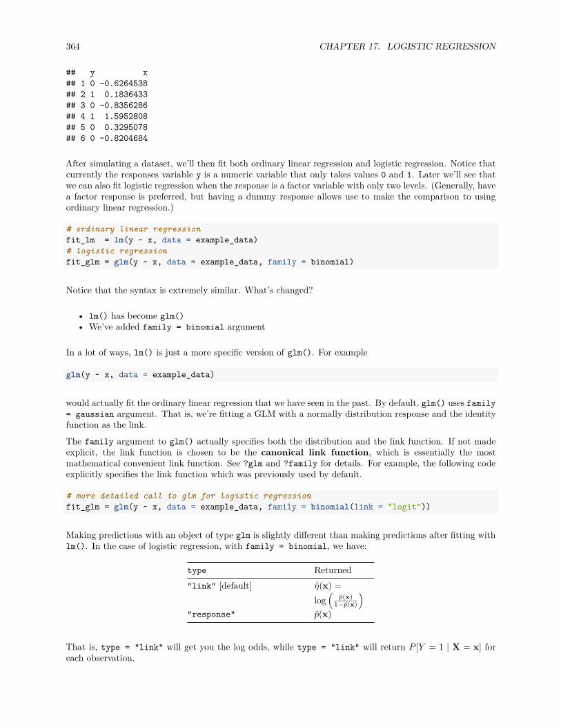
364 CHAPTER 17. LOGISTIC REGRESSION
## y x## 1 0 -0.6264538## 2 1 0.1836433## 3 0 -0.8356286## 4 1 1.5952808## 5 0 0.3295078## 6 0 -0.8204684
After simulating a dataset, we’ll then fit both ordinary linear regression and logistic regression. Notice thatcurrently the responses variable y is a numeric variable that only takes values 0 and 1. Later we’ll see thatwe can also fit logistic regression when the response is a factor variable with only two levels. (Generally, havea factor response is preferred, but having a dummy response allows use to make the comparison to usingordinary linear regression.)
# ordinary linear regressionfit_lm = lm(y ~ x, data = example_data)# logistic regressionfit_glm = glm(y ~ x, data = example_data, family = binomial)
Notice that the syntax is extremely similar. What’s changed?
• lm() has become glm()• We’ve added family = binomial argument
In a lot of ways, lm() is just a more specific version of glm(). For example
glm(y ~ x, data = example_data)
would actually fit the ordinary linear regression that we have seen in the past. By default, glm() uses family= gaussian argument. That is, we’re fitting a GLM with a normally distribution response and the identityfunction as the link.
The family argument to glm() actually specifies both the distribution and the link function. If not madeexplicit, the link function is chosen to be the canonical link function, which is essentially the mostmathematical convenient link function. See ?glm and ?family for details. For example, the following codeexplicitly specifies the link function which was previously used by default.
# more detailed call to glm for logistic regressionfit_glm = glm(y ~ x, data = example_data, family = binomial(link = "logit"))
Making predictions with an object of type glm is slightly different than making predictions after fitting withlm(). In the case of logistic regression, with family = binomial, we have:
type Returned"link" [default] η(x) =
log(
p(x)1−p(x)
)"response" p(x)
That is, type = "link" will get you the log odds, while type = "link" will return P [Y = 1 | X = x] foreach observation.
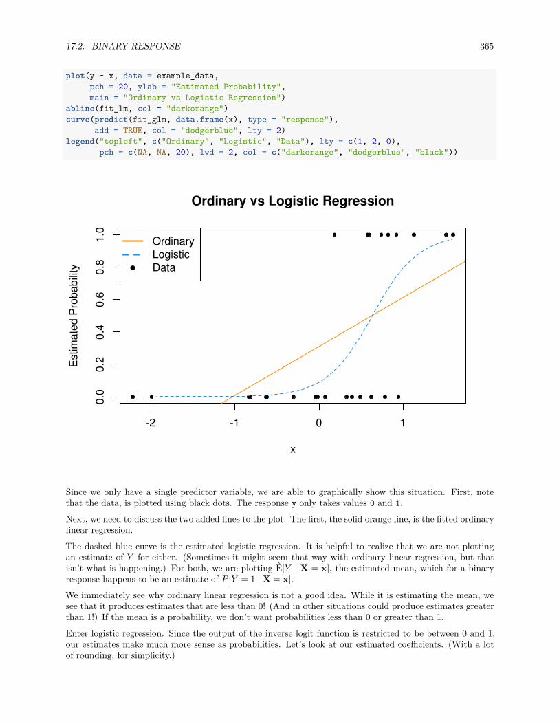
17.2. BINARY RESPONSE 365
plot(y ~ x, data = example_data,pch = 20, ylab = "Estimated Probability",main = "Ordinary vs Logistic Regression")
abline(fit_lm, col = "darkorange")curve(predict(fit_glm, data.frame(x), type = "response"),
add = TRUE, col = "dodgerblue", lty = 2)legend("topleft", c("Ordinary", "Logistic", "Data"), lty = c(1, 2, 0),
pch = c(NA, NA, 20), lwd = 2, col = c("darkorange", "dodgerblue", "black"))
-2 -1 0 1
0.0
0.2
0.4
0.6
0.8
1.0
Ordinary vs Logistic Regression
x
Est
imat
ed P
roba
bilit
y
OrdinaryLogisticData
Since we only have a single predictor variable, we are able to graphically show this situation. First, notethat the data, is plotted using black dots. The response y only takes values 0 and 1.
Next, we need to discuss the two added lines to the plot. The first, the solid orange line, is the fitted ordinarylinear regression.
The dashed blue curve is the estimated logistic regression. It is helpful to realize that we are not plottingan estimate of Y for either. (Sometimes it might seem that way with ordinary linear regression, but thatisn’t what is happening.) For both, we are plotting E[Y | X = x], the estimated mean, which for a binaryresponse happens to be an estimate of P [Y = 1 | X = x].
We immediately see why ordinary linear regression is not a good idea. While it is estimating the mean, wesee that it produces estimates that are less than 0! (And in other situations could produce estimates greaterthan 1!) If the mean is a probability, we don’t want probabilities less than 0 or greater than 1.
Enter logistic regression. Since the output of the inverse logit function is restricted to be between 0 and 1,our estimates make much more sense as probabilities. Let’s look at our estimated coefficients. (With a lotof rounding, for simplicity.)

366 CHAPTER 17. LOGISTIC REGRESSION
round(coef(fit_glm), 1)
## (Intercept) x## -2.3 3.7
Our estimated model is then:
log(
p(x)1 − p(x)
)= −2.3 + 3.7x
Because we’re not directly estimating the mean, but instead a function of the mean, we need to be carefulwith our interpretation of β1 = 3.7. This means that, for a one unit increase in x, the log odds change (inthis case increase) by 3.7. Also, since β1 is positive, as we increase x we also increase p(x). To see how much,we have to consider the inverse logistic function.For example, we have:
P [Y = 1 | X = −0.5] = e−2.3+3.7·(−0.5)
1 + e−2.3+3.7·(−0.5) ≈ 0.016
P [Y = 1 | X = 0] = e−2.3+3.7·(0)
1 + e−2.3+3.7·(0) ≈ 0.09112296
P [Y = 1 | X = 1] = e−2.3+3.7·(1)
1 + e−2.3+3.7·(1) ≈ 0.8021839
Now that we know we should use logistic regression, and not ordinary linear regression, let’s consider anotherexample. This time, let’s consider the model
log(
p(x)1 − p(x)
)= 1 + −4x.
Again, we could re-write this to better match the function we’re using to simulate the data:
Yi ∼ Bern(pi)pi = p(xi) = 11 + e−η(xi)
η(xi) = 1 + −4xi
In this model, as x increases, the log odds decrease.
set.seed(1)example_data = sim_logistic_data(sample_size = 50, beta_0 = 1, beta_1 = -4)
We again simulate some observations form this model, then fit logistic regression.
fit_glm = glm(y ~ x, data = example_data, family = binomial)
plot(y ~ x, data = example_data,pch = 20, ylab = "Estimated Probability",main = "Logistic Regression, Decreasing Probability")
curve(predict(fit_glm, data.frame(x), type = "response"),add = TRUE, col = "dodgerblue", lty = 2)
legend("bottomleft", c("Estimated Probability", "Data"), lty = c(2, 0),pch = c(NA, 20), lwd = 2, col = c("dodgerblue", "black"))
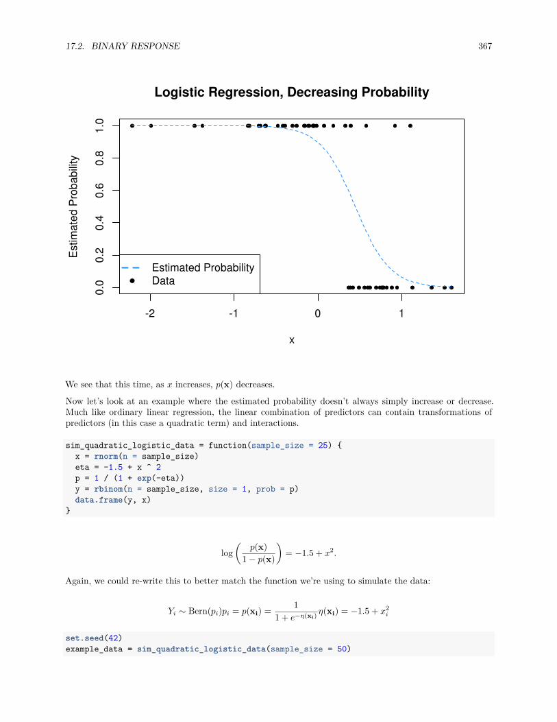
17.2. BINARY RESPONSE 367
-2 -1 0 1
0.0
0.2
0.4
0.6
0.8
1.0
Logistic Regression, Decreasing Probability
x
Est
imat
ed P
roba
bilit
y
Estimated ProbabilityData
We see that this time, as x increases, p(x) decreases.
Now let’s look at an example where the estimated probability doesn’t always simply increase or decrease.Much like ordinary linear regression, the linear combination of predictors can contain transformations ofpredictors (in this case a quadratic term) and interactions.
sim_quadratic_logistic_data = function(sample_size = 25) {x = rnorm(n = sample_size)eta = -1.5 + x ^ 2p = 1 / (1 + exp(-eta))y = rbinom(n = sample_size, size = 1, prob = p)data.frame(y, x)
}
log(
p(x)1 − p(x)
)= −1.5 + x2.
Again, we could re-write this to better match the function we’re using to simulate the data:
Yi ∼ Bern(pi)pi = p(xi) = 11 + e−η(xi)
η(xi) = −1.5 + x2i
set.seed(42)example_data = sim_quadratic_logistic_data(sample_size = 50)
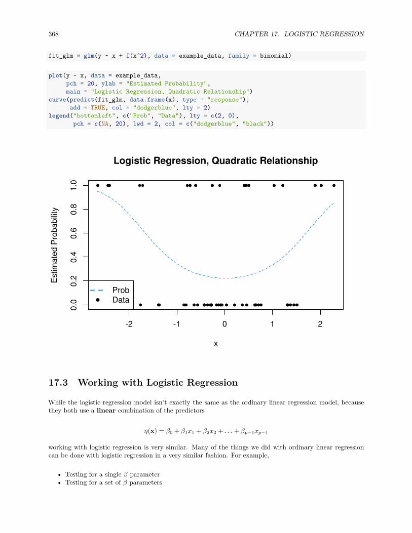
368 CHAPTER 17. LOGISTIC REGRESSION
fit_glm = glm(y ~ x + I(x^2), data = example_data, family = binomial)
plot(y ~ x, data = example_data,pch = 20, ylab = "Estimated Probability",main = "Logistic Regression, Quadratic Relationship")
curve(predict(fit_glm, data.frame(x), type = "response"),add = TRUE, col = "dodgerblue", lty = 2)
legend("bottomleft", c("Prob", "Data"), lty = c(2, 0),pch = c(NA, 20), lwd = 2, col = c("dodgerblue", "black"))
-2 -1 0 1 2
0.0
0.2
0.4
0.6
0.8
1.0
Logistic Regression, Quadratic Relationship
x
Est
imat
ed P
roba
bilit
y
ProbData
17.3 Working with Logistic Regression
While the logistic regression model isn’t exactly the same as the ordinary linear regression model, becausethey both use a linear combination of the predictors
η(x) = β0 + β1x1 + β2x2 + . . . + βp−1xp−1
working with logistic regression is very similar. Many of the things we did with ordinary linear regressioncan be done with logistic regression in a very similar fashion. For example,
• Testing for a single β parameter• Testing for a set of β parameters
17.3. WORKING WITH LOGISTIC REGRESSION 369
• Formula specification in R.• Interpreting parameters and estimates• Confidence intervals for parameters• Confidence intervals for mean response• Variable selection
After some introduction to the new tests, we’ll demonstrate each of these using an example.
17.3.1 Testing with GLMs
Like ordinary linear regression, we’ll want to be able to perform hypothesis testing. We’ll again want bothsingle parameter, and multiple parameter tests.
17.3.2 Wald Test
In ordinary linear regression, we performed the test of
H0 : βj = 0 vs H1 : βj = 0
using a t-test.
For the logistic regression model,
log(
p(x)1 − p(x)
)= β0 + β1x1 + . . . + βp−1xp−1
we can again perform a test of
H0 : βj = 0 vs H1 : βj = 0
however, the test statistic and its distribution are no longer t. We see that the test statistic takes the sameform
z = βj − βj
SE[βj ]approx∼ N(0, 1)
but now we are performing a z-test, as the test statistics follows an approximate standard normal distribution,provided we have a large enough sample. (The t-test for ordinary linear regression, assuming the assumptionswere correct, had an exact distribution for any sample size.)
We’ll skip some of the exact details of the calculations, as R will obtain the standard error for us. The useof this test will be extremely similar to the t-test for ordinary linear regression. Essentially the only thingthat changes is the distribution of the test statistic.
17.3.3 Likelihood-Ratio Test
Consider the following full model,
log(
p(xi)1 − p(xi)
)= β0 + β1xi1 + β2xi2 + · · · + β(p−1)xi(p−1) + ϵi

370 CHAPTER 17. LOGISTIC REGRESSION
This model has p−1 predictors, for a total of p β-parameters. We will denote the MLE of these β-parametersas βFull
Now consider a null (or reduced) model,
log(
p(xi)1 − p(xi)
)= β0 + β1xi1 + β2xi2 + · · · + β(q−1)xi(q−1) + ϵi
where q < p. This model has q − 1 predictors, for a total of q β-parameters. We will denote the MLE ofthese β-parameters as βNull
The difference between these two models can be codified by the null hypothesis of a test.
H0 : βq = βq+1 = · · · = βp−1 = 0.
We then define a test statistic, D,
D = −2 log
(L(βNull)L(βFull)
)= 2 log
(L(βFull)L(βNull)
)= 2
(ℓ(βFull) − ℓ(βNull)
)where L denotes a likelihood and ℓ denotes a log-likelihood. For a large enough sample, this test statistichas an approximate Chi-square distribution
Dapprox∼ χ2
k
where k = p − q, the different in number of parameters of the two models.
This test, which we will call the Likelihood-Ratio Test, will be the analogue to the ANOVA F -test forlogistic regression. Interestingly, to perform the Likelihood-Ratio Test, we’ll actually again use the anova()function in R!.
The Likelihood-Ratio Test is actually a rather general test, however, here we have presented a specificapplication to nested logistic regression models.
17.3.4 SAheart Example
To illustrate the use of logistic regression, we will use the SAheart dataset from the ElemStatLearn package.
# install.packages("ElemStatLearn")library(ElemStatLearn)data("SAheart")
sbp tobacco ldl adiposity famhist typea obesity alcohol age chd160 12.00 5.73 23.11 Present 49 25.30 97.20 52 1144 0.01 4.41 28.61 Absent 55 28.87 2.06 63 1118 0.08 3.48 32.28 Present 52 29.14 3.81 46 0170 7.50 6.41 38.03 Present 51 31.99 24.26 58 1134 13.60 3.50 27.78 Present 60 25.99 57.34 49 1132 6.20 6.47 36.21 Present 62 30.77 14.14 45 0
This data comes from a retrospective sample of males in a heart-disease high-risk region of the WesternCape, South Africa. The chd variables, which we will use as a response, indicates whether or not coronaryheart disease is present in an individual. Note that this is coded as a numeric 0 / 1 variable. Using this asa response with glm() it is important to indicate family = binomial, otherwise ordinary linear regression
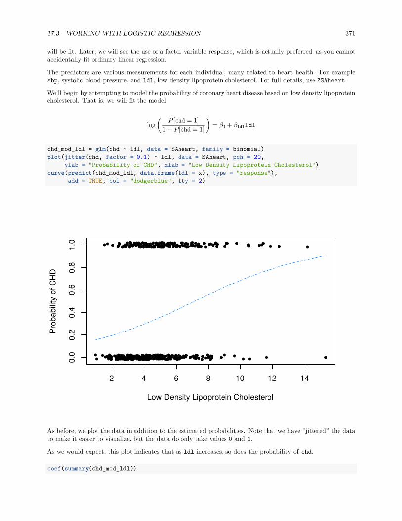
17.3. WORKING WITH LOGISTIC REGRESSION 371
will be fit. Later, we will see the use of a factor variable response, which is actually preferred, as you cannotaccidentally fit ordinary linear regression.
The predictors are various measurements for each individual, many related to heart health. For examplesbp, systolic blood pressure, and ldl, low density lipoprotein cholesterol. For full details, use ?SAheart.
We’ll begin by attempting to model the probability of coronary heart disease based on low density lipoproteincholesterol. That is, we will fit the model
log(
P [chd = 1]1 − P [chd = 1]
)= β0 + βldlldl
chd_mod_ldl = glm(chd ~ ldl, data = SAheart, family = binomial)plot(jitter(chd, factor = 0.1) ~ ldl, data = SAheart, pch = 20,
ylab = "Probability of CHD", xlab = "Low Density Lipoprotein Cholesterol")curve(predict(chd_mod_ldl, data.frame(ldl = x), type = "response"),
add = TRUE, col = "dodgerblue", lty = 2)
2 4 6 8 10 12 14
0.0
0.2
0.4
0.6
0.8
1.0
Low Density Lipoprotein Cholesterol
Pro
babi
lity
of C
HD
As before, we plot the data in addition to the estimated probabilities. Note that we have “jittered” the datato make it easier to visualize, but the data do only take values 0 and 1.
As we would expect, this plot indicates that as ldl increases, so does the probability of chd.
coef(summary(chd_mod_ldl))

372 CHAPTER 17. LOGISTIC REGRESSION
## Estimate Std. Error z value Pr(>|z|)## (Intercept) -1.9686681 0.27307908 -7.209150 5.630207e-13## ldl 0.2746613 0.05163983 5.318787 1.044615e-07
To perform the test
H0 : βldl = 0
we use the summary() function as we have done so many times before. Like the t-test for ordinary linearregression, this returns the estimate of the parameter, its standard error, the relevant test statistic (z), andits p-value. Here we have an incredibly low p-value, so we reject the null hypothesis. ldl appears to be asignificant predictor.
When fitting logistic regression, we can use the same formula syntax as ordinary linear regression. So, to fitan additive model using all available predictors, we use:
chd_mod_additive = glm(chd ~ ., data = SAheart, family = binomial)
We can then use the likelihood-ratio test to compare the two model. Specifically, we are testing
H0 : βsbp = βtobacco = βadiposity = βfamhist = βtypea = βobesity = βalcohol = βage = 0
We could manually calculate the test statistic,
-2 * as.numeric(logLik(chd_mod_ldl) - logLik(chd_mod_additive))
## [1] 92.13879
Or we could utilize the anova() function. By specifying test = "LRT", R will use the likelihood-ratio testto compare the two models.
anova(chd_mod_ldl, chd_mod_additive, test = "LRT")
## Analysis of Deviance Table#### Model 1: chd ~ ldl## Model 2: chd ~ sbp + tobacco + ldl + adiposity + famhist + typea + obesity +## alcohol + age## Resid. Df Resid. Dev Df Deviance Pr(>Chi)## 1 460 564.28## 2 452 472.14 8 92.139 < 2.2e-16 ***## ---## Signif. codes: 0 '***' 0.001 '**' 0.01 '*' 0.05 '.' 0.1 ' ' 1
We see that the test statistic that we had just calculated appears in the output. The very small p-valuesuggests that we prefer the larger model.
While we prefer the additive model compared to the model with only a single predictor, do we actually needall of the predictors in the additive model? To select a subset of predictors, we can use a stepwise procedureas we did with ordinary linear regression. Recall that AIC and BIC were defined in terms of likelihoods.Here we demonstrate using AIC with a backwards selection procedure.
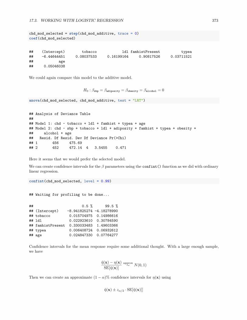
17.3. WORKING WITH LOGISTIC REGRESSION 373
chd_mod_selected = step(chd_mod_additive, trace = 0)coef(chd_mod_selected)
## (Intercept) tobacco ldl famhistPresent typea## -6.44644451 0.08037533 0.16199164 0.90817526 0.03711521## age## 0.05046038
We could again compare this model to the additive model.
H0 : βsbp = βadiposity = βobesity = βalcohol = 0
anova(chd_mod_selected, chd_mod_additive, test = "LRT")
## Analysis of Deviance Table#### Model 1: chd ~ tobacco + ldl + famhist + typea + age## Model 2: chd ~ sbp + tobacco + ldl + adiposity + famhist + typea + obesity +## alcohol + age## Resid. Df Resid. Dev Df Deviance Pr(>Chi)## 1 456 475.69## 2 452 472.14 4 3.5455 0.471
Here it seems that we would prefer the selected model.
We can create confidence intervals for the β parameters using the confint() function as we did with ordinarylinear regression.
confint(chd_mod_selected, level = 0.99)
## Waiting for profiling to be done...
## 0.5 % 99.5 %## (Intercept) -8.941825274 -4.18278990## tobacco 0.015704975 0.14986616## ldl 0.022923610 0.30784590## famhistPresent 0.330033483 1.49603366## typea 0.006408724 0.06932612## age 0.024847330 0.07764277
Confidence intervals for the mean response require some additional thought. With a large enough sample,we have
η(x) − η(x)SE[η(x)]
approx∼ N(0, 1)
Then we can create an approximate (1 − α)% confidence intervals for η(x) using
η(x) ± zα/2 · SE[η(x)]]

374 CHAPTER 17. LOGISTIC REGRESSION
where zα/2 is the critical value such that P (Z > zα/2) = α/2.
This isn’t a particularly interesting interval. Instead, what we really want is an interval for the mean response,p(x). To obtain an interval for p(x), we simply apply the inverse logit transform to the endpoints of theinterval for η.
(logit−1(η(x) − zα/2 · SE[η(x)]), logit−1(η(x) + zα/2 · SE[η(x)])
)To demonstrate creating these intervals, we’ll consider a new observation.
new_obs = data.frame(sbp = 148.0,tobacco = 5,ldl = 12,adiposity = 31.23,famhist = "Present",typea = 47,obesity = 28.50,alcohol = 23.89,age = 60
)
Fist, we’ll use the predict() function to obtain η(x) for this observation.
eta_hat = predict(chd_mod_selected, new_obs, se.fit = TRUE, type = "link")eta_hat
## $fit## 1## 1.579545#### $se.fit## [1] 0.4114796#### $residual.scale## [1] 1
By setting se.fit = TRUE, R also computes SE[η].
z_crit = round(qnorm(0.975), 2)round(z_crit, 2)
## [1] 1.96
After obtaining the correct critical value, we can easily create a 95% confidence interval for η(x).
eta_hat$fit + c(-1, 1) * z_crit * eta_hat$se.fit
## [1] 0.773045 2.386045
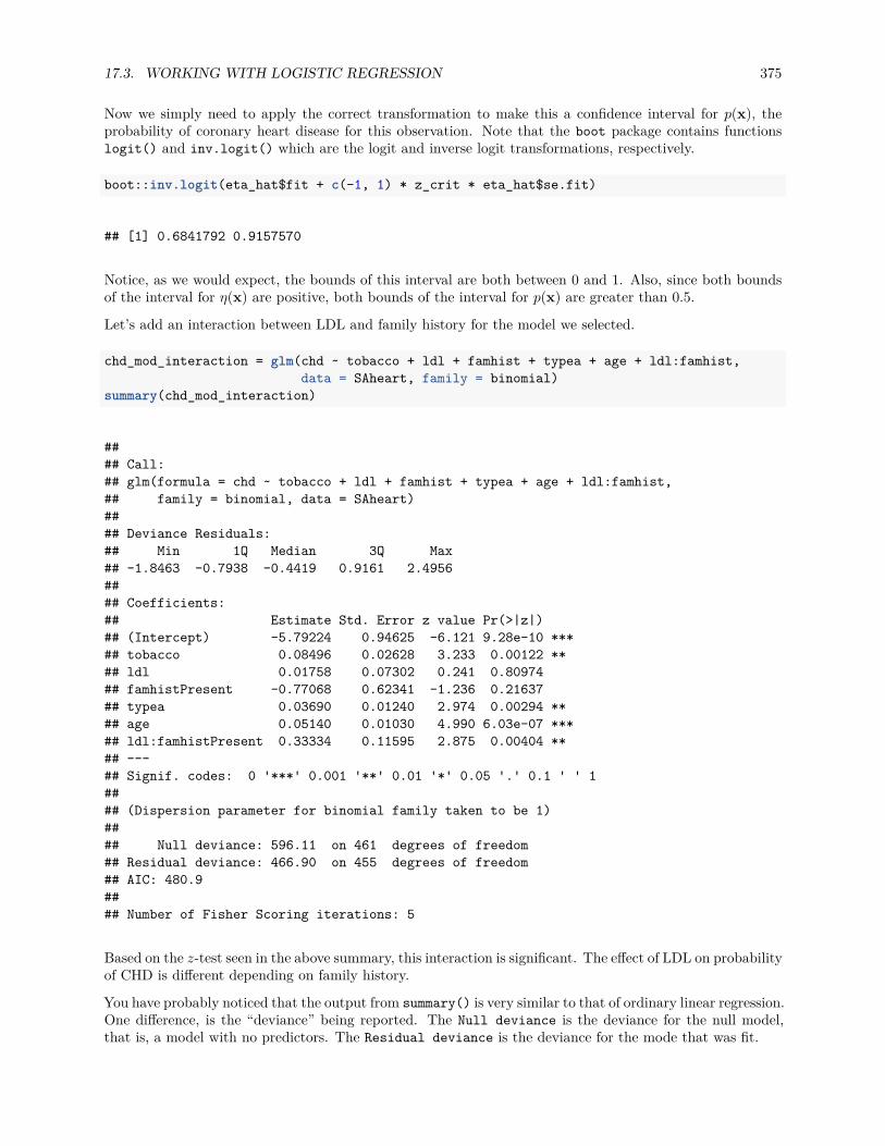
17.3. WORKING WITH LOGISTIC REGRESSION 375
Now we simply need to apply the correct transformation to make this a confidence interval for p(x), theprobability of coronary heart disease for this observation. Note that the boot package contains functionslogit() and inv.logit() which are the logit and inverse logit transformations, respectively.
boot::inv.logit(eta_hat$fit + c(-1, 1) * z_crit * eta_hat$se.fit)
## [1] 0.6841792 0.9157570
Notice, as we would expect, the bounds of this interval are both between 0 and 1. Also, since both boundsof the interval for η(x) are positive, both bounds of the interval for p(x) are greater than 0.5.
Let’s add an interaction between LDL and family history for the model we selected.
chd_mod_interaction = glm(chd ~ tobacco + ldl + famhist + typea + age + ldl:famhist,data = SAheart, family = binomial)
summary(chd_mod_interaction)
#### Call:## glm(formula = chd ~ tobacco + ldl + famhist + typea + age + ldl:famhist,## family = binomial, data = SAheart)#### Deviance Residuals:## Min 1Q Median 3Q Max## -1.8463 -0.7938 -0.4419 0.9161 2.4956#### Coefficients:## Estimate Std. Error z value Pr(>|z|)## (Intercept) -5.79224 0.94625 -6.121 9.28e-10 ***## tobacco 0.08496 0.02628 3.233 0.00122 **## ldl 0.01758 0.07302 0.241 0.80974## famhistPresent -0.77068 0.62341 -1.236 0.21637## typea 0.03690 0.01240 2.974 0.00294 **## age 0.05140 0.01030 4.990 6.03e-07 ***## ldl:famhistPresent 0.33334 0.11595 2.875 0.00404 **## ---## Signif. codes: 0 '***' 0.001 '**' 0.01 '*' 0.05 '.' 0.1 ' ' 1#### (Dispersion parameter for binomial family taken to be 1)#### Null deviance: 596.11 on 461 degrees of freedom## Residual deviance: 466.90 on 455 degrees of freedom## AIC: 480.9#### Number of Fisher Scoring iterations: 5
Based on the z-test seen in the above summary, this interaction is significant. The effect of LDL on probabilityof CHD is different depending on family history.
You have probably noticed that the output from summary() is very similar to that of ordinary linear regression.One difference, is the “deviance” being reported. The Null deviance is the deviance for the null model,that is, a model with no predictors. The Residual deviance is the deviance for the mode that was fit.
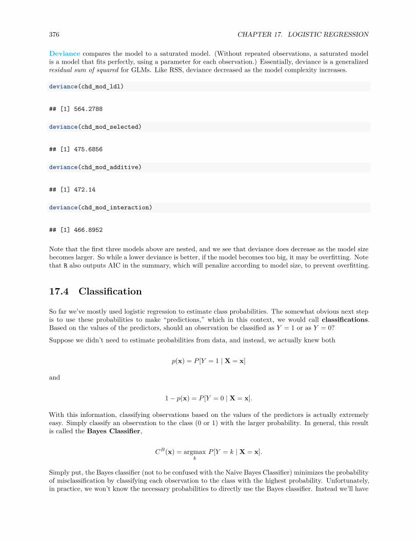
376 CHAPTER 17. LOGISTIC REGRESSION
Deviance compares the model to a saturated model. (Without repeated observations, a saturated modelis a model that fits perfectly, using a parameter for each observation.) Essentially, deviance is a generalizedresidual sum of squared for GLMs. Like RSS, deviance decreased as the model complexity increases.
deviance(chd_mod_ldl)
## [1] 564.2788
deviance(chd_mod_selected)
## [1] 475.6856
deviance(chd_mod_additive)
## [1] 472.14
deviance(chd_mod_interaction)
## [1] 466.8952
Note that the first three models above are nested, and we see that deviance does decrease as the model sizebecomes larger. So while a lower deviance is better, if the model becomes too big, it may be overfitting. Notethat R also outputs AIC in the summary, which will penalize according to model size, to prevent overfitting.
17.4 Classification
So far we’ve mostly used logistic regression to estimate class probabilities. The somewhat obvious next stepis to use these probabilities to make “predictions,” which in this context, we would call classifications.Based on the values of the predictors, should an observation be classified as Y = 1 or as Y = 0?
Suppose we didn’t need to estimate probabilities from data, and instead, we actually knew both
p(x) = P [Y = 1 | X = x]
and
1 − p(x) = P [Y = 0 | X = x].
With this information, classifying observations based on the values of the predictors is actually extremelyeasy. Simply classify an observation to the class (0 or 1) with the larger probability. In general, this resultis called the Bayes Classifier,
CB(x) = argmaxk
P [Y = k | X = x].
Simply put, the Bayes classifier (not to be confused with the Naive Bayes Classifier) minimizes the probabilityof misclassification by classifying each observation to the class with the highest probability. Unfortunately,in practice, we won’t know the necessary probabilities to directly use the Bayes classifier. Instead we’ll have
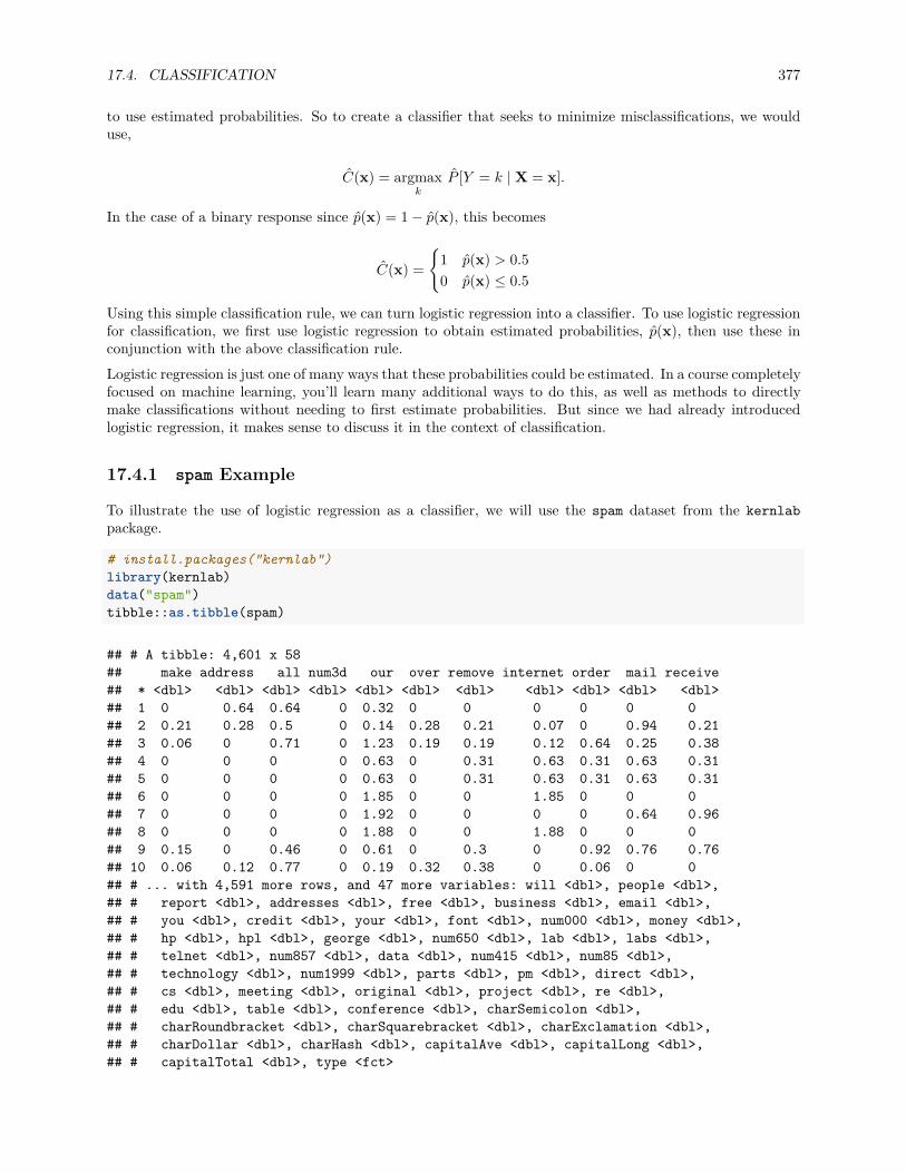
17.4. CLASSIFICATION 377
to use estimated probabilities. So to create a classifier that seeks to minimize misclassifications, we woulduse,
C(x) = argmaxk
P [Y = k | X = x].
In the case of a binary response since p(x) = 1 − p(x), this becomes
C(x) =
{1 p(x) > 0.50 p(x) ≤ 0.5
Using this simple classification rule, we can turn logistic regression into a classifier. To use logistic regressionfor classification, we first use logistic regression to obtain estimated probabilities, p(x), then use these inconjunction with the above classification rule.Logistic regression is just one of many ways that these probabilities could be estimated. In a course completelyfocused on machine learning, you’ll learn many additional ways to do this, as well as methods to directlymake classifications without needing to first estimate probabilities. But since we had already introducedlogistic regression, it makes sense to discuss it in the context of classification.
17.4.1 spam Example
To illustrate the use of logistic regression as a classifier, we will use the spam dataset from the kernlabpackage.
# install.packages("kernlab")library(kernlab)data("spam")tibble::as.tibble(spam)
## # A tibble: 4,601 x 58## make address all num3d our over remove internet order mail receive## * <dbl> <dbl> <dbl> <dbl> <dbl> <dbl> <dbl> <dbl> <dbl> <dbl> <dbl>## 1 0 0.64 0.64 0 0.32 0 0 0 0 0 0## 2 0.21 0.28 0.5 0 0.14 0.28 0.21 0.07 0 0.94 0.21## 3 0.06 0 0.71 0 1.23 0.19 0.19 0.12 0.64 0.25 0.38## 4 0 0 0 0 0.63 0 0.31 0.63 0.31 0.63 0.31## 5 0 0 0 0 0.63 0 0.31 0.63 0.31 0.63 0.31## 6 0 0 0 0 1.85 0 0 1.85 0 0 0## 7 0 0 0 0 1.92 0 0 0 0 0.64 0.96## 8 0 0 0 0 1.88 0 0 1.88 0 0 0## 9 0.15 0 0.46 0 0.61 0 0.3 0 0.92 0.76 0.76## 10 0.06 0.12 0.77 0 0.19 0.32 0.38 0 0.06 0 0## # ... with 4,591 more rows, and 47 more variables: will <dbl>, people <dbl>,## # report <dbl>, addresses <dbl>, free <dbl>, business <dbl>, email <dbl>,## # you <dbl>, credit <dbl>, your <dbl>, font <dbl>, num000 <dbl>, money <dbl>,## # hp <dbl>, hpl <dbl>, george <dbl>, num650 <dbl>, lab <dbl>, labs <dbl>,## # telnet <dbl>, num857 <dbl>, data <dbl>, num415 <dbl>, num85 <dbl>,## # technology <dbl>, num1999 <dbl>, parts <dbl>, pm <dbl>, direct <dbl>,## # cs <dbl>, meeting <dbl>, original <dbl>, project <dbl>, re <dbl>,## # edu <dbl>, table <dbl>, conference <dbl>, charSemicolon <dbl>,## # charRoundbracket <dbl>, charSquarebracket <dbl>, charExclamation <dbl>,## # charDollar <dbl>, charHash <dbl>, capitalAve <dbl>, capitalLong <dbl>,## # capitalTotal <dbl>, type <fct>

378 CHAPTER 17. LOGISTIC REGRESSION
This dataset, created in the late 1990s at Hewlett-Packard Labs, contains 4601 emails, of which 1813 areconsidered spam. The remaining are not spam. (Which for simplicity, we might call, ham.) Additionaldetails can be obtained by using ?spam of by visiting the UCI Machine Learning Repository.
The response variable, type, is a factor with levels that label each email as spam or nonspam. When fittingmodels, nonspam will be the reference level, Y = 0, as it comes first alphabetically.
is.factor(spam$type)
## [1] TRUE
levels(spam$type)
## [1] "nonspam" "spam"
Many of the predictors (often called features in machine learning) as engineered based on the emails. Forexample, charDollar is the number of times an email contains the $ character. Some variables are highlyspecific to this dataset, for example george and num650. (The name and area code for one of the researcherswhose emails were used.) We should keep in mind that this dataset was created based on emails send toacademic type researcher in the 1990s. Any results we derive probably won’t generalize to modern emailsfor the general public.
To get started, we’ll first test-train split the data.
set.seed(42)# spam_idx = sample(nrow(spam), round(nrow(spam) / 2))spam_idx = sample(nrow(spam), 1000)spam_trn = spam[spam_idx, ]spam_tst = spam[-spam_idx, ]
We’ve used a somewhat small train set relative to the total size of the dataset. In practice it should likelybe larger, but this is simply to keep training time low for illustration and rendering of this document.
fit_caps = glm(type ~ capitalTotal, data = spam_trn, family = binomial)fit_selected = glm(type ~ edu + money + capitalTotal + charDollar, data = spam_trn, family = binomial)fit_additive = glm(type ~ ., data = spam_trn, family = binomial)fit_over = glm(type ~ capitalTotal * (.), data = spam_trn, family = binomial, maxit = 50)
We’ll fit four logistic regression, each more complex than the previous. Note that we’re suppressing twowarnings. The first we briefly mentioned previously.
## Warning: glm.fit: fitted probabilities numerically 0 or 1 occurred
Note that, when we receive this warning, we should be highly suspicious of the parameter estimates.
coef(fit_selected)
## (Intercept) edu money capitalTotal charDollar## -1.1248423316 -3.4811734345 1.0303968430 0.0009187823 12.3988576908

17.4. CLASSIFICATION 379
However, the model can still be used to create a classifier, and we will evaluate that classifier on its ownmerits.
We also, “suppressed” the warning:
## Warning: glm.fit: algorithm did not converge
In reality, we didn’t actually suppress it, but instead changed maxit to 50, when fitting the model fit_over.This was enough additional iterations to allow the iteratively reweighted least squares algorithm to convergewhen fitting the model.
17.4.2 Evaluating Classifiers
The metric we’ll be most interested in for evaluating the overall performance of a classifier is the misclas-sification rate. (Sometimes, instead accuracy is reported, which is instead the proportion of correctionclassifications, so both metrics serve the same purpose.)
Misclass(C, Data) = 1n
n∑i=1
I(yi = C(xi))
I(yi = C(x)) =
{0 yi = C(x)1 yi = C(x)
When using this metric on the training data, it will have the same issues as RSS did for ordinary linearregression, that is, it will only go down.
# training misclassification ratemean(ifelse(predict(fit_caps) > 0, "spam", "nonspam") != spam_trn$type)
## [1] 0.342
mean(ifelse(predict(fit_selected) > 0, "spam", "nonspam") != spam_trn$type)
## [1] 0.212
mean(ifelse(predict(fit_additive) > 0, "spam", "nonspam") != spam_trn$type)
## [1] 0.064
mean(ifelse(predict(fit_over) > 0, "spam", "nonspam") != spam_trn$type)
## [1] 0.063
Because of this, training data isn’t useful for evaluating, as it would suggest that we should always use thelargest possible model, when in reality, that model is likely overfitting. Recall, a model that is too complexwill overfit. A model that is too simple will underfit. (We’re looking for something in the middle.)
To overcome this, we’ll use cross-validation as we did with ordinary linear regression, but this time we’llcross-validate the misclassification rate. To do so, we’ll use the cv.glm() function from the boot library. It

380 CHAPTER 17. LOGISTIC REGRESSION
takes arguments for the data (in this case training), a model fit via glm(), and K, the number of folds. See?cv.glm for details.
Previously, for cross-validating RMSE in ordinary linear regression, we used LOOCV. We certainly could dothat here. However, with logistic regression, we no longer have the clever trick that would allow use to obtaina LOOCV metric without needing to fit the model n times. So instead, we’ll use 5-fold cross-validation. (5and 10 fold are the most common in practice.) Instead of leaving a single observation out repeatedly, we’llleave out a fifth of the data.
Essentially we’ll repeat the following process 5 times:
• Randomly set aside a fifth of the data (each observation will only be held-out once)• Train model on remaining data• Evaluate misclassification rate on held-out data
The 5-fold cross-validated misclassification rate will be the average of these misclassification rates. By onlyneeding to refit the model 5 times, instead of n times, we will save a lot of computation time.
library(boot)set.seed(1)cv.glm(spam_trn, fit_caps, K = 5)$delta[1]
## [1] 0.2138392
cv.glm(spam_trn, fit_selected, K = 5)$delta[1]
## [1] 0.1522741
cv.glm(spam_trn, fit_additive, K = 5)$delta[1]
## [1] 0.07346089
cv.glm(spam_trn, fit_over, K = 5)$delta[1]
## [1] 0.11
Note that we’re suppressing warnings again here. (Now there would be a lot more, since were fitting a totalof 20 models.)
Based on these results, fit_caps and fit_selected are underfitting relative to fit_additive. Similarly,fit_over is overfitting relative to fit_additive. Thus, based on these results, we prefer the classifiercreated based on the logistic regression fit and stored in fit_additive.
Going forward, to evaluate and report on the efficacy of this classifier, we’ll use the test dataset. We’regoing to take the position that the test data set should never be used in training, which is why we usedcross-validation within the training dataset to select a model. Even though cross-validation uses hold-outsets to generate metrics, at some point all of the data is used for training.
To quickly summarize how well this classifier works, we’ll create a confusion matrix.
It further breaks down the classification errors into false positives and false negatives.

17.4. CLASSIFICATION 381
Figure 17.1: Confusion Matrix
make_conf_mat = function(predicted, actual) {table(predicted = predicted, actual = actual)
}
Let’s explicitly store the predicted values of our classifier on the test dataset.
spam_tst_pred = ifelse(predict(fit_additive, spam_tst) > 0, "spam", "nonspam")spam_tst_pred = ifelse(predict(fit_additive, spam_tst, type = "response") > 0.5, "spam", "nonspam")
The previous two lines of code produce the same output, that is the same predictions, since
η(x) = 0 ⇐⇒ p(x) = 0.5
Now we’ll use these predictions to create a confusion matrix.
(conf_mat_50 = make_conf_mat(predicted = spam_tst_pred, actual = spam_tst$type))
## actual## predicted nonspam spam## nonspam 2050 161## spam 137 1253
Prev = PTotal Obs = TP + FN
Total Obs
table(spam_tst$type) / nrow(spam_tst)
#### nonspam spam## 0.6073313 0.3926687
First, note that to be a reasonable classifier, it needs to outperform the obvious classifier of simply clas-sifying all observations to the majority class. In this case, classifying everything as non-spam for a testmisclassification rate of 0.3926687
Next, we can see that using the classifier create from fit_additive, only a total of 137 + 161 = 298 fromthe total of 3601 email in the test set are misclassified. Overall, the accuracy in the test set it
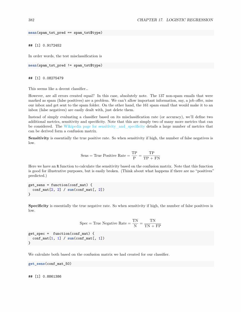
382 CHAPTER 17. LOGISTIC REGRESSION
mean(spam_tst_pred == spam_tst$type)
## [1] 0.9172452
In order words, the test misclassification is
mean(spam_tst_pred != spam_tst$type)
## [1] 0.08275479
This seems like a decent classifier…
However, are all errors created equal? In this case, absolutely note. The 137 non-spam emails that weremarked as spam (false positives) are a problem. We can’t allow important information, say, a job offer, missour inbox and get sent to the spam folder. On the other hand, the 161 spam email that would make it to aninbox (false negatives) are easily dealt with, just delete them.
Instead of simply evaluating a classifier based on its misclassification rate (or accuracy), we’ll define twoadditional metrics, sensitivity and specificity. Note that this are simply two of many more metrics that canbe considered. The Wikipedia page for sensitivity_and_specificity details a large number of metrics thatcan be derived form a confusion matrix.
Sensitivity is essentially the true positive rate. So when sensitivity if high, the number of false negatives islow.
Sens = True Positive Rate = TPP = TP
TP + FN
Here we have an R function to calculate the sensitivity based on the confusion matrix. Note that this functionis good for illustrative purposes, but is easily broken. (Think about what happens if there are no “positives”predicted.)
get_sens = function(conf_mat) {conf_mat[2, 2] / sum(conf_mat[, 2])
}
Specificity is essentially the true negative rate. So when sensitivity if high, the number of false positives islow.
Spec = True Negative Rate = TNN = TN
TN + FP
get_spec = function(conf_mat) {conf_mat[1, 1] / sum(conf_mat[, 1])
}
We calculate both based on the confusion matrix we had created for our classifier.
get_sens(conf_mat_50)
## [1] 0.8861386

17.4. CLASSIFICATION 383
get_spec(conf_mat_50)
## [1] 0.9373571
Recall that we had created this classifier using a probability of 0.5 as a “cutoff” for how observations shouldbe classified. Now we’ll modify this cutoff. We’ll see that by modifying the cutoff, c, we can improvesensitivity or specificity at the expense of the overall accuracy (misclassification rate).
C(x) =
{1 p(x) > c
0 p(x) ≤ c
Additionally, if we change the cutoff to improve sensitivity, we’ll decrease specificity, and vice versa.
First let’s see what happens when we lower the cutoff from 0.5 to 0.1 to create a new classifier, and thusnew predictions.
spam_tst_pred_10 = ifelse(predict(fit_additive, spam_tst, type = "response") > 0.1, "spam", "nonspam")
This is essentially decreasing the threshold for an email to be labeled as spam, so far more emails will belabeled as spam. We see that in the following confusion matrix.
(conf_mat_10 = make_conf_mat(predicted = spam_tst_pred_10, actual = spam_tst$type))
## actual## predicted nonspam spam## nonspam 1654 31## spam 533 1383
Unfortunately, while this does greatly reduce false negatives, false positives have almost quadrupled. We seethis reflected in the sensitivity and specificity.
get_sens(conf_mat_10)
## [1] 0.9780764
get_spec(conf_mat_10)
## [1] 0.7562872
This classifier, using 0.1 instead of 0.5 has a higher sensitivity, but a much lower specificity. Clearly, weshould have moved the cutoff in the other direction. Let’s try 0.9.
spam_tst_pred_90 = ifelse(predict(fit_additive, spam_tst, type = "response") > 0.9, "spam", "nonspam")
This is essentially increasing the threshold for an email to be labeled as spam, so far fewer emails will belabeled as spam. Again, we see that in the following confusion matrix.

384 CHAPTER 17. LOGISTIC REGRESSION
(conf_mat_90 = make_conf_mat(predicted = spam_tst_pred_90, actual = spam_tst$type))
## actual## predicted nonspam spam## nonspam 2120 447## spam 67 967
This is the results we’re looking for. We have far fewer false positives. While sensitivity is greatly reduced,specificity has gone up.
get_sens(conf_mat_90)
## [1] 0.6838755
get_spec(conf_mat_90)
## [1] 0.9693644
While this is far fewer false positives, is it acceptable though? Still probably not. Also, don’t forget, thiswould actually be a terrible spam detector today since this is based on data from a very different era of theinternet, for a very specific set of people. Spam has changed a lot since 90s! (Ironically, machine learning isprobably partially to blame.)
This chapter has provided a rather quick introduction to classification, and thus, machine learning. For amore complete coverage of machine learning, An Introduction to Statistical Learning is a highly recommendedresource. Additionally, R for Statistical Learning has been written as a supplement which provides additionaldetail on how to perform these methods using R. The classification and logistic regression chapters might beuseful.
We should note that the code to perform classification using logistic regression is presented in a way thatillustrates the concepts to the reader. In practice, you may to prefer to use a more general machine learningpipeline such as caret in R. This will streamline processes for creating predictions and generating evaluationmetrics.

Chapter 18
Beyond
“End? No, the journey doesn’t end here.”— J.R.R. Tolkien
After reading this chapter you will be able to:
• Understand the roadmap to continued education about models and the R programming language.
18.1 What’s Next
So you’ve completed STAT 420, where do you go from here? Now that you understand the basics of linearmodeling, there is a wide world of applied statistics waiting to be explored. We’ll briefly detail some resourcesand discuss how they relate to what you have learned in STAT 420.
18.2 RStudio
RStudio has recently released version 1.0! This is exciting for a number of reason, especially the releaseof R Notebooks. R Notebooks combine the RMarkdown you have already learned with the ability to workinteractively.
18.3 Tidy Data
In this textbook, much of the data we have seen has been nice and tidy. It was rectangular where each rowis an observation and each column is a variable. This is not always the case! Many packages have beendeveloped to deal with data, and force it into a nice format, which is called tidy data, that we can then usefor modeling. Often during analysis, this is where a large portion of your time will be spent.
The R community has started to call this collection of packages the Tidyverse. It was once called theHadleyverse, as Hadley Wickham has authored so many of the packages. Hadley is writing a book called Rfor Data Science which describes the use of many of these packages. (And also how to use some to make themodeling process better!) This book is a great starting point for diving deeper into the R community. Thetwo main packages are dplyr and tidyr both of which are used internally in RStudio.
385

386 CHAPTER 18. BEYOND
18.4 Visualization
In this course, we have mostly used the base plotting methods in R. When working with tidy data, manyusers prefer to use the ggplot2 package, also developed by Hadley Wickham. RStudio provides a ratherdetailed “cheat sheet” for working with ggplot2. The community maintains a graph gallery of examples.
Use of the manipulate package with RStudio gives the ability to quickly change a static graphic to becomeinteractive.
18.5 Web Applications
RStudio has made it incredible easy to create data products through the use of Shiny, which allows for thecreation of web applications with R. RStudio maintains an ever-growing tutorial and gallery of examples.
18.6 Experimental Design
In the ANOVA chapter, we briefly discussed experimental design. This topic could easily be its own class,and is currently an area of revitalized interest with the rise of A/B testing. Two more classic statisticalreferences include Statistics for Experimenters by Box, Hunter, and Hunter as well as Design and Analysisof Experiments by Douglas Montgomery. There are several R packages for design of experiments, list in theCRAN Task View.
18.7 Machine Learning
Using models for prediction is the key focus of machine learning. There are many methods, each with its ownpackage, however R has a wonderful package called caret, Classification And REgression Training, whichprovides a unified interface to training these models. It also contains various utilities for data processingand visualization that are useful for predictive modeling.
Applied Predictive Modeling by Max Kuhn, the author of the caret package is a good general resource forpredictive modeling, which obviously utilizes R. An Introduction to Statistical Learning by James, Witten,Hastie, and Tibshirani is a gentle introduction to machine learning from a statistical perspective which uses Rand picks up right where this courses stops. This is based on the often referenced The Elements of StatisticalLearning by Hastie, Tibshirani, and Friedman. Both are freely available online.
18.7.1 Deep Learning
While, it probably isn’t the best tool for the job, R now has the ability to train deep neural networks viaTensorFlow.
18.8 Time Series
In this class we have only considered independent data. What if data is dependent? Time Series is the areaof statistics which deals with this issue, and could easily span multiple courses.
Two books that are used in STAT 429 at the University of Illinois, both free:
• Time Series Analysis and Its Applications: With R Examples by Shumway and Stoffer

18.9. BAYESIANISM 387
• A Tour of Time Series Analysis with R by Balamuta, Guerrier, Molinari, and Xu. This book is currentlyunder development at UIUC.
Some tutorials:
• Little Book of R for Time Series• Quick R: Time Series and Forecasting• TSA: Start to Finish Examples
When performing time series analysis in R you should be aware of the many packages that are useful foranalysis. It should be hard to avoid the forecast and zoo packages. Often the most difficult part will bedealing with time and date data. Make sure you are utilizing one of the many packages that help with this.
18.9 Bayesianism
In this class, we have worked within the frequentist view of statistics. There is an entire alternative universeof Bayesian statistics.
Doing Bayesian Data Analysis: A Tutorial with R, JAGS, and Stan by John Kruschke is a great introductionto the topic. It introduces the world of probabilistic programming, in particular Stan, which can be used inboth R and Python.
18.10 High Performance Computing
Often R will be called a “slow” language, for two reasons. One, because many do not understand R. Two,because sometimes it really is. Luckily, it is easy to extend R via the Rcpp package to allow for faster code.Many modern R packages utilize Rcpp to achieve better performance.
18.11 Further R Resources
Also, don’t forget that previously in this book we have outlined a large number of R resources. Now thatyou’ve gotten started with R many of these will be much more useful.
If any of these topics interest you, and you would like more information, please don’t hesitate to start adiscussion on the forums!
:)

388 CHAPTER 18. BEYOND

Chapter 19
Appendix
389