Applying Adomian Decomposition Method toSolve Burgess Equation with a Non-linear

Source

O. Gonzalez-Gaxiola∗, R. Bernal-JaquezDepartamento de Matematicas Aplicadas y Sistema,sUniversidad Autonoma Metropolitana-Cuajimalpa,

C.P. 05300 Mexico, D.F., Mexico

AbstractIn the present work we consider the mathematical model that describes braintumour growth (glioblastomas) under medical treatment. Based on the med-ical study presented by R. Stupp et al. (New Engl Journal of Med 352: 987-996, 2005) which evidence that, combined therapies such as, radiotherapyand chemotherapy, produces negative tumour-growth, and using the mathe-matical model of P. K. Burgess et al. (J Neuropath and Exp Neur 56: 704-713, 1997) as an starting point, we present a model for tumour growth undermedical treatment represented by a non-linear partial differential equationthat is solved using the Adomian Decomposition Method (ADM). It is alsoshown that the non-linear term efficiently models the effects of the combinedtherapies. By means of a proper use of parameters, this model could be usedfor calculating doses in radiotherapy and chemotherapy.

Keywords: Burgess equation, Adomian polynomials, Glioblastoma, Temozolo-mide.

IntroductionThe glioblastoma, also known as glioblastoma multiforme (GBM), is a highlyinvasive glioma in the brain [23]. It is the most common and most aggressive brain∗ogonzalez@correo.cua.uam.mx

1

arX

iv:1

606.

0025

9v1

[q-

bio.

TO

] 1

4 Ja

n 20

16

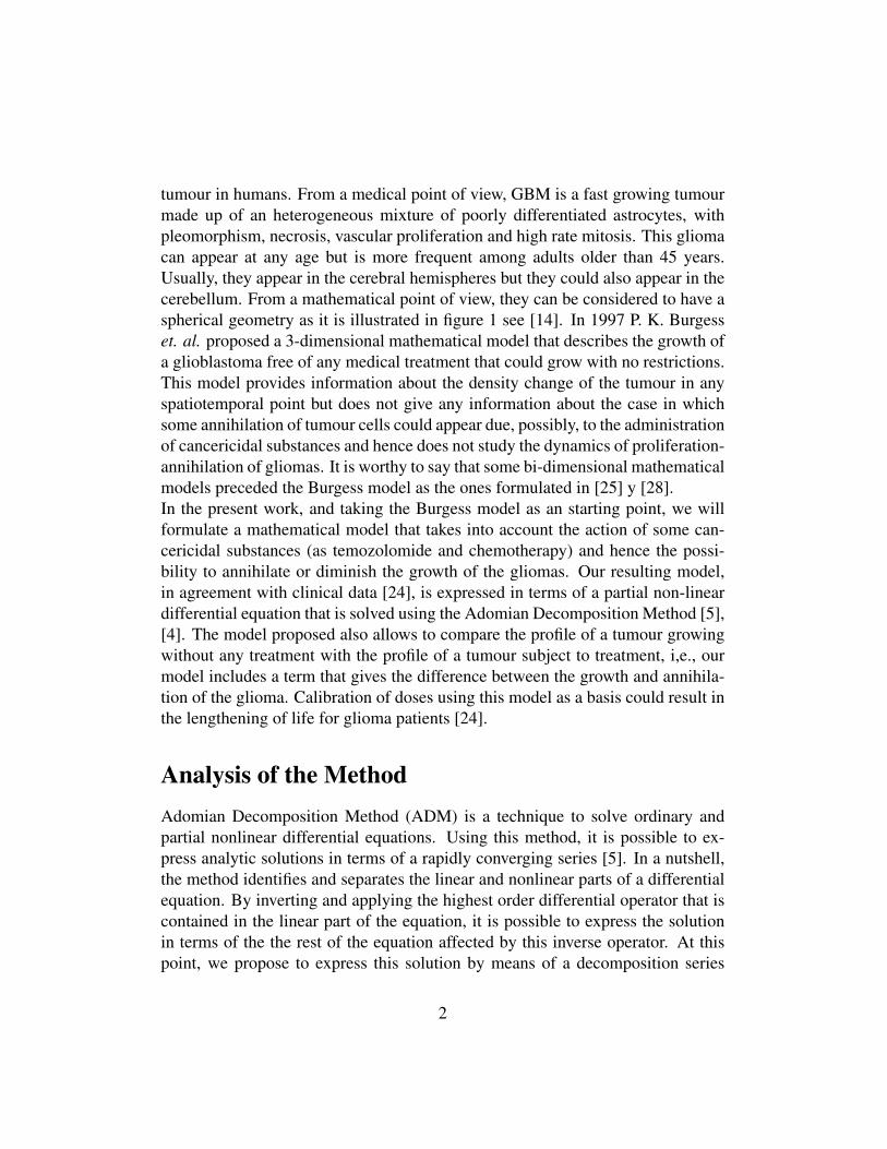
tumour in humans. From a medical point of view, GBM is a fast growing tumourmade up of an heterogeneous mixture of poorly differentiated astrocytes, withpleomorphism, necrosis, vascular proliferation and high rate mitosis. This gliomacan appear at any age but is more frequent among adults older than 45 years.Usually, they appear in the cerebral hemispheres but they could also appear in thecerebellum. From a mathematical point of view, they can be considered to have aspherical geometry as it is illustrated in figure 1 see [14]. In 1997 P. K. Burgesset. al. proposed a 3-dimensional mathematical model that describes the growth ofa glioblastoma free of any medical treatment that could grow with no restrictions.This model provides information about the density change of the tumour in anyspatiotemporal point but does not give any information about the case in whichsome annihilation of tumour cells could appear due, possibly, to the administrationof cancericidal substances and hence does not study the dynamics of proliferation-annihilation of gliomas. It is worthy to say that some bi-dimensional mathematicalmodels preceded the Burgess model as the ones formulated in [25] y [28].In the present work, and taking the Burgess model as an starting point, we willformulate a mathematical model that takes into account the action of some can-cericidal substances (as temozolomide and chemotherapy) and hence the possi-bility to annihilate or diminish the growth of the gliomas. Our resulting model,in agreement with clinical data [24], is expressed in terms of a partial non-lineardifferential equation that is solved using the Adomian Decomposition Method [5],[4]. The model proposed also allows to compare the profile of a tumour growingwithout any treatment with the profile of a tumour subject to treatment, i,e., ourmodel includes a term that gives the difference between the growth and annihila-tion of the glioma. Calibration of doses using this model as a basis could result inthe lengthening of life for glioma patients [24].

Analysis of the MethodAdomian Decomposition Method (ADM) is a technique to solve ordinary andpartial nonlinear differential equations. Using this method, it is possible to ex-press analytic solutions in terms of a rapidly converging series [5]. In a nutshell,the method identifies and separates the linear and nonlinear parts of a differentialequation. By inverting and applying the highest order differential operator that iscontained in the linear part of the equation, it is possible to express the solutionin terms of the the rest of the equation affected by this inverse operator. At thispoint, we propose to express this solution by means of a decomposition series

2

Figura 1: Illustration of a glioblastoma tumour in the parietal lobe.

with terms that will be well determined by recursion and that gives rise to thesolution components. The nonlinear part is expressed in terms of the Adomianpolynomials. The initial or the boundary condition and the terms that contain theindependent variables will be considered as the initial approximation. In this wayand by means of a recurrence relations, it is possible to calculate the terms of theseries by recursion that gives the approximate solution of the differential equation.

Given a partial (or ordinary) differential equation

Fu(x, t) = g(x, t) (1)

with the initial conditionu(x,0) = f (x), (2)

where F is differential operator that could itself, in general, be nonlinear andtherefore includes linear and nonlinear terms.In general, equation (1) is be written as

Ltu(x, t)+Ru(x, t)+Nu(x, t) = g(x, t) (3)

where Lt =∂

∂ t , R is the linear remainder operator that could include partial deriva-tives with respect to x, N is a nonlinear operator which is presumed to be analytic

3

and g is a non-homogeneous term that is independent of the solution u.Solving for Ltu(x, t), we have

Ltu(x, t) = g(x, t)−Ru(x, t)−Nu(x, t). (4)

As L is presumed to be invertible, we can apply L−1t (·) =

∫ t0(·)dt to both sides of

equation (4) obtaining

L−1t Ltu(x, t) = L−1

t g(x, t)−L−1t Ru(x, t)−L−1

t Nu(x, t). (5)

An equivalent expression to (5) is

u(x, t) = f (x)+L−1t g(x, t)−L−1

t Ru(x, t)−L−1t Nu(x, t), (6)

where f (x) is the constant of integration with respect to t that satisfies Lt f = 0. Inequations where the initial value t = t0, we can conveniently define L−1.The ADM proposes a decomposition series solution u(x, t) given as

u(x, t) =∞

∑n=0

un(x, t). (7)

The nonlinear term Nu(x, t) is given as

Nu(x, t) =∞

∑n=0

An(u0,u1, . . . ,un) (8)

where {An}∞n=0 is the Adomian polynomials sequence given by (see deduction in

appendix at the end of this paper)

An =1n!

dn

dλ n [N(n

∑k=0

λkuk)]|λ=0. (9)

Substituting (7), (8) y (9) into equation (6), we obtain∞

∑n=0

un(x, t) = f (x)+L−1t g(x, t)−L−1

t R∞

∑n=0

un(x, t)−L−1t

∞

∑n=0

An(u0,u1, . . . ,un),

(10)with u0 identified as f (x)+L−1

t g(x, t), and therefore, we can write

u0(x, t) = f (x)+L−1t g(x, t),

u1(x, t) = −L−1t Ru0(x, t)−L−1

t A0(u0),...

un+1(x, t) = −L−1t Run(x, t)−L−1

t An(u0, . . . ,un).

4

From which we can establish the following recurrence relation, that is obtained ina explicit way for instance in reference [27],{

u0(x, t) = f (x)+L−1t g(x, t),

un+1(x, t) =−L−1t Run(x, t)−L−1

t An(u0,u1, . . . ,un), n = 0,1,2, . . . .(11)

Using (11), we can obtain an approximate solution of (1), (2) as

u(x, t)≈k

∑n=0

un(x, t), where limk→∞

k

∑n=0

un(x, t) = u(x, t). (12)

This method has been successfully applied to a large class of both linear and non-linear problems [13]. The Adomian decomposition method requires far less workin comparison with traditional methods. This method considerably decreases thevolume of calculations. The decomposition procedure of Adomian easily obtainsthe solution without linearising the problem by implementing the decompositionmethod rather than the standard methods. In this approach, the solution is foundin the form of a convergent series with easily computed components; in manycases, the convergence of this series is extremely fast and consequently only afew terms are needed in order to have an idea of how the solutions behave. Con-vergence conditions of this series have been investigated by several authors, e.g.,[1, 2, 8, 9].

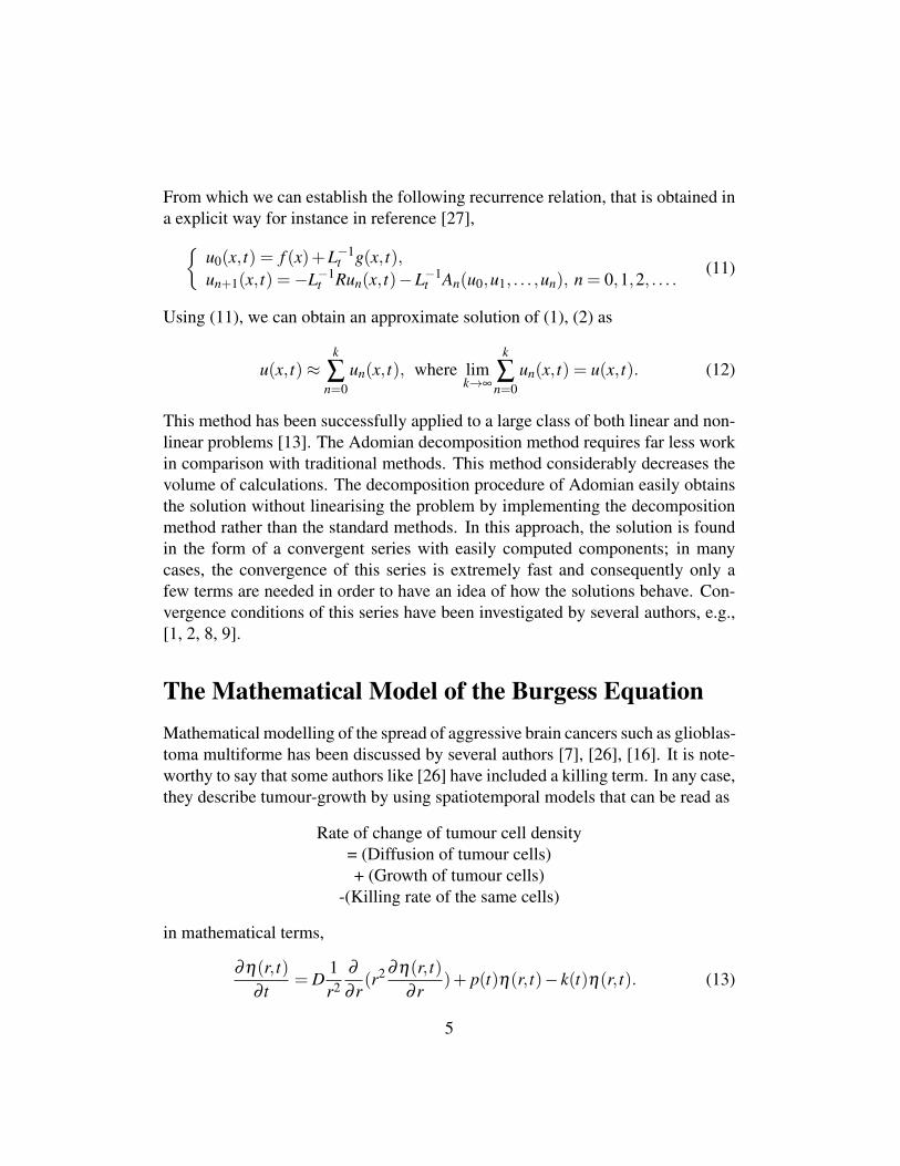
The Mathematical Model of the Burgess EquationMathematical modelling of the spread of aggressive brain cancers such as glioblas-toma multiforme has been discussed by several authors [7], [26], [16]. It is note-worthy to say that some authors like [26] have included a killing term. In any case,they describe tumour-growth by using spatiotemporal models that can be read as

Rate of change of tumour cell density= (Diffusion of tumour cells)+ (Growth of tumour cells)

-(Killing rate of the same cells)

in mathematical terms,

∂η(r, t)∂ t

= D1r2

∂

∂ r(r2 ∂η(r, t)

∂ r)+ p(t)η(r, t)− k(t)η(r, t). (13)

5

In this equation, η(r, t) is the concentration of tumour cells at location r at timet, D is the diffusion coefficient, i.e. a measure of the areal speed of the invadingglioblastoma cells, p is the rate of reproduction of the glioblastoma cells, and kthe killing rate of the same cells. The last term has been used by some authorsto investigate the effects of chemotherapy [25], [28]. In this model, the tumouris assumed to have spherical symmetry and the medium through which it is ex-panding, to be isotropic and uniform. We can assume that at the beginning of time(diagnostic time t0), the density of cancer cells is N0, i. e., η(r0, t0) = N0 and sothe equation (13) is{

∂η(r,t)∂ t = D(r, t)

(∂ 2η(r,t)

∂ r2 + 2r

∂η(r,t)∂ r

)+[p(t)− k(t)]η(r, t),

η(r0, t0) = N0.(14)

The solution of (14) is given, without many details, in [7] and in [15]. They solvethis equation for the -non-very realistic- case in which k(t)≡ 0 and p(t) and D(r, t)are constants. The solution for this case is given by

η(r, t) =N0e{pt− r2

4Dt }

8(πDt)32

. (15)

Using this equation (15), the mentioned authors calculate the expected survivaltime (in months) for a person that has a brain tumour modelled using equation(14).Following [6], we propose the change of variables τ = 2Dt, u(r,τ) = rη(r, t) andω(r,τ) = p−k

2D . Using this change of variables and keeping D constant, equation(14) is given by

∂u(r,τ)∂τ

=12

∂ 2u(r,τ)∂ r2 +

ω(r,τ)2D

. (16)

In [24], a medical study is presented that stresses the advantages of using com-bined therapies such as chemotherapy and radiotherapy in the treatment of braincancer. Concretely, they present the results of using temozolomide in combina-tion with radiotherapy. The results show a lengthening in the patient life as aconsequence of the tumour size decrease. Mathematically this is traduced as anegative growth of the tumour, in other words, the term p(r, t)− k(r, t) (growth ofthe cancer cells minus eliminations of cancer cells) is negative. In present work,we will study the case presented by Roger Stupp et. al. in [24]. Our model willmake use of equation (16) taking D constant and (r,τ) ∈ (0,1]× [0,1] that gives arenormalised time and space intervals. In order to take into account the combined

6

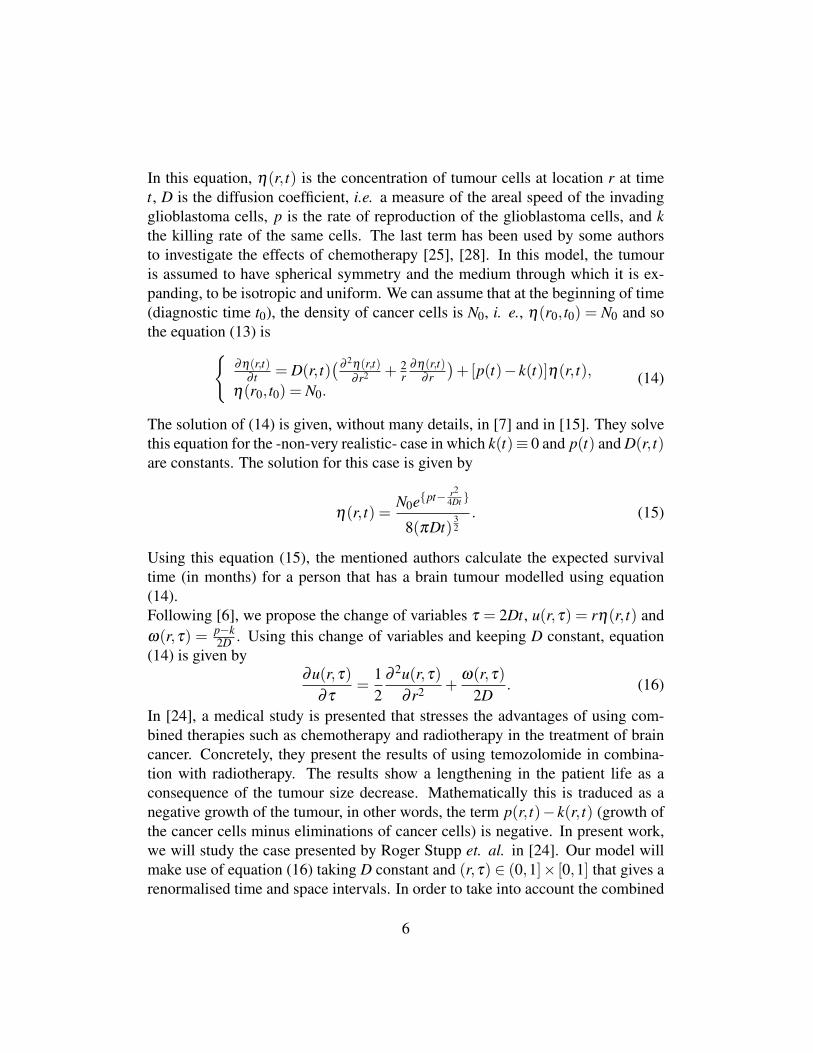
effects of radiotherapy and chemotherapy, we will introduce a term that modelsthe decay (negative growth) of the glioma, ω(r,τ) = e−u+ 1

2e−2u, with u= u(r,τ).The decrease of the tumour depending on the position r and time τ as it shown infigure 2.

0.0

0.5

1.0

0.0

0.5

1.0

0.0

0.5

1.0

1.5

2.0

Figura 2: ω(r,τ) = e−u + 12 e−2u with (r,τ) ∈ (0,1]× [0,1]

The ADM has been used by several authors to solve linear and non-linear dif-fusion equations as well as fractional diffusion equations, some important refer-ences can be found in [10, 11, 12, 17, 18, 19, 20, 21, 22]. In the present work weare interested in the solution of the diffusion equation (16) in which a non-linearsource ω(r,τ) is modelling the effects of the combined use of radiotherapy andchemotherapy treatment with Temozolomide as is reported in [24].

Solution of a nonlinear modelConsidering the equation (16), with ω(r,τ) = e−u + 1

2e−2u and D = 12 our model

will be given by the following non-linear partial differential equation

7

{∂u∂τ

= 12

∂ 2u∂ r2 + e−u + 1

2e−2u,

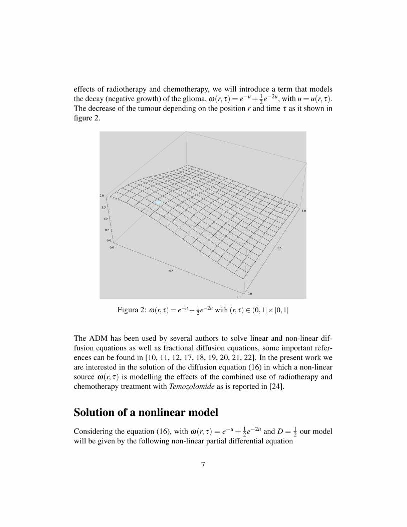
u(r,0) = ln(r+2).(17)

In equation (17) we have made the a priori assumption that the initial conditionis u(r,0) = ln(r + 2). This assumption considers that the initial tumour growthprofile is given by u(r,0) in the time we start the annihilation or attenuation ofthe gliomas by means of some treatment (as chemotherapy). The initial growthprofile is illustrated in figure 3.

0.2 0.4 0.6 0.8 1.0

0.8

0.9

1.0

1.1

Figura 3: Initial growth-profile u(r,0) = ln(r+2)

Using

An(u0,u1, . . . ,un) =1n!

dn

dαn [N(n

∑k=0

αkuk)]|α=0 n≥ 0

to calculate the Adomian polynomials, we have :

A0(u0) = N(u0) = e−u0 +12

e−2u0

A1(u0,u1) = N′(u0)u1 =−u1e−u0−u1e−2u0

A2(u0,u1,u2) = N′′(u0)u2

12! +N′(u0)u2

=u2

12 (e−u0 +2e−2u0)+u2(−e−u0− e−2u0)

8

A3(u0,u1,u2,u3) = N′′′(u0)u3

13!

+N′′(u0)u1u2 +N′(u0)u3

=u3

16(−e−u0−4e−2u0)+u1u2(e−u0 +2e−2u0)−u3(e−u0 + e−2u0)

....

Using the sequence for {An}∞n=0 and the recurrence relation given in (11) we can

calculate {un}, in this way:u0 = ln(r+2)

u1 =∫ t

0[− 1

2(r+2)2 + e−u0 +12

e−2u0]dt =t

r+2....

The partial sums of the Adomian series are

S0 = u0 = ln(r+2)

S1 = u0 +u1 = ln(r+2)+τ

r+2

S2 = u0 +u1 +u2 = ln(r+2)+τ

r+2− τ2

2(r+2)2

S3 = u0 +u1 +u2 +u3 = ln(r+2)+τ

r+2− τ2

2(r+2)2 +τ3

3(r+2)3

...

Sm = u0 +u1 + . . .+um = ln(r+2)+τ

r+2− τ2

2(r+2)2 + . . .+(−1)m+1τm

m(r+2)m

and taking into account the equation (12), we have

u(r,τ) = ln(r+2)+τ

r+2− τ2

2(r+2)2 + . . .+(−1)m+1τm

m(r+2)m + · · · (18)

taking the sum of the first terms, we can see that the above series converges toln( τ+r+2

r+2 ). Then, using (18) we have

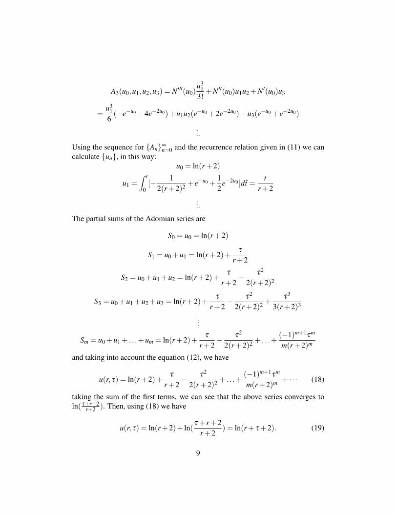
u(r,τ) = ln(r+2)+ ln(τ + r+2

r+2) = ln(r+ τ +2). (19)

9

0.0

0.5

1.0

0.0

0.5

1.0

0.8

1.0

1.2

1.4

Figura 4: u(r,τ) = ln(r+ τ +2) with (r,τ) ∈ (0,1]× [0,1]

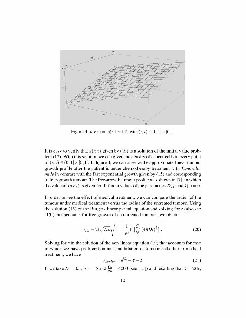
It is easy to verify that u(r,τ) given by (19) is a solution of the initial value prob-lem (17). With this solution we can given the density of cancer cells in every pointof (r,τ)∈ (0,1]× [0,1]. In figure 4, we can observe the approximate-linear tumourgrowth-profile after the patient is under chemotherapy treatment with Temozolo-mide in contrast with the fast exponential growth given by (15) and correspondingto free-growth tumour. The free-growth tumour profile was shown in [7], in whichthe value of η(r, t) is given for different values of the parameters D, p and k(t)= 0.

In order to see the effect of medical treatment, we can compare the radius of thetumour under medical treatment versus the radius of the untreated tumour. Usingthe solution (15) of the Burgess linear partial equation and solving for r (also see[15]) that accounts for free growth of an untreated tumour , we obtain

rlin = 2t√

Dp

√∣∣∣∣1− 1pt

ln[C0

N0(4πDt)

32 ]

∣∣∣∣. (20)

Solving for r in the solution of the non-linear equation (19) that accounts for casein which we have proliferation and annihilation of tumour cells due to medicaltreatment, we have

rnonlin = eN0− τ−2 (21)

If we take D = 0.5, p = 1.5 and C0N0

= 4000 (see [15]) and recalling that τ = 2Dt,

10

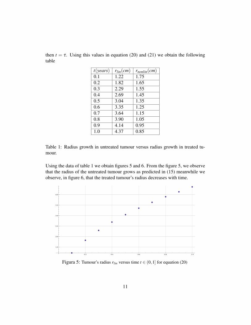
then t = τ . Using this values in equation (20) and (21) we obtain the followingtable

t(years) rlin(cm) rnonlin(cm)0.1 1.22 1.750.2 1.82 1.650.3 2.29 1.550.4 2.69 1.450.5 3.04 1.350.6 3.35 1.250.7 3.64 1.150.8 3.90 1.050.9 4.14 0.951.0 4.37 0.85

Table 1: Radius growth in untreated tumour versus radius growth in treated tu-mour.

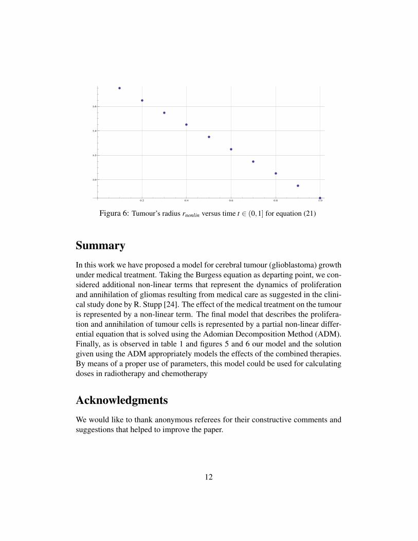
Using the data of table 1 we obtain figures 5 and 6. From the figure 5, we observethat the radius of the untreated tumour grows as predicted in (15) meanwhile weobserve, in figure 6, that the treated tumour’s radius decreases with time.

0.2 0.4 0.6 0.8 1.0

1.5

2.0

2.5

3.0

3.5

4.0

Figura 5: Tumour’s radius rlin versus time t ∈ (0,1] for equation (20)

11

0.2 0.4 0.6 0.8 1.0

1.0

1.2

1.4

1.6

Figura 6: Tumour’s radius rnonlin versus time t ∈ (0,1] for equation (21)

SummaryIn this work we have proposed a model for cerebral tumour (glioblastoma) growthunder medical treatment. Taking the Burgess equation as departing point, we con-sidered additional non-linear terms that represent the dynamics of proliferationand annihilation of gliomas resulting from medical care as suggested in the clini-cal study done by R. Stupp [24]. The effect of the medical treatment on the tumouris represented by a non-linear term. The final model that describes the prolifera-tion and annihilation of tumour cells is represented by a partial non-linear differ-ential equation that is solved using the Adomian Decomposition Method (ADM).Finally, as is observed in table 1 and figures 5 and 6 our model and the solutiongiven using the ADM appropriately models the effects of the combined therapies.By means of a proper use of parameters, this model could be used for calculatingdoses in radiotherapy and chemotherapy

AcknowledgmentsWe would like to thank anonymous referees for their constructive comments andsuggestions that helped to improve the paper.

12

Appendix: Adomian polynomialsIn this appendix we will deduce equation (9) that accounts for every term in thesuccession of the Adomian Polynomials assuming the following hypotheses statedin [9]:

(i) the series solution, u = ∑∞n=0 un , of the problem given in equation (1) is

absolutely convergent,

(ii) The non-linear function N(u) can be expressed by means of a power serieswhose radio of convergence is infinite, that is

N(u) =∞

∑n=0

N(n)(0)un

n!, |u|< ∞. (22)

Assuming the above hypotheses, the series whose terms are the Adomian Polyno-mials {An}∞

n=0 results to be a generalisation of the Taylor’s series

N(u) =∞

∑n=0

An(u0,u1, . . . ,un) =∞

∑n=0

N(n)(u0)(u−u0)

n

n!. (23)

Is worthy to note that (23) is a rearranged expression of the series (22), and notethat, due to hypothesis, this series is convergent. Consider now, the parametrisa-tion proposed by G. Adomian in [3] given by

uλ (x, t) =∞

∑n=0

un(x, t) f n(λ ), (24)

where λ is a parameter in R and f is a complex-valued function such that | f |< 1.With this choosing of f and using the hypotheses above stated, the series (24) isabsolutely convergent.Substituting (24) in (23), we obtain

N(uλ ) =∞

∑n=0

N(n)(u0)

(∑

∞j=1 u j(x, t) f j(λ )

)n

n!. (25)

Due to the absolute convergence of

∞

∑j=1

u j(x, t) f j(λ ), (26)

13

we can rearrange N(uλ ) in order to obtain the series of the form ∑∞n=0 An f n(λ ).

Using (25) we can obtain the coefficients Ak de f k(λ ), and finally we deduce theAdomian’s polynomials. That is,

N(uλ ) = N(u0)+N(1)(u0)(u1 f (λ )+u2 f 2(λ )+u3 f 3(λ )+ . . .

)+

N(2)(u0)

2!(u1 f (λ )+u2 f 2(λ )+u3 f 3(λ )+ . . .

)2

+N(3)(u0)

3!(u1 f (λ )+u2 f 2(λ )+u3 f 3(λ )+ . . .

)3+ . . .

+N(4)(u0)

4!(u1 f (λ )+u2 f 2(λ )+u3 f 3(λ )+ . . .

)3+ . . .

= N(u0)+N(1)(u0)u1 f (λ )+(

N(1)(u0)u2 +N(2)(u0)u2

12!

)f 2(λ )

+

(N(1)(u0)u3 +N(2)(u0)u1u2 +N(3)(u0)

u31

3!

)f 3(λ )+ . . .

=∞

∑n=0

An(u0,u1, . . . ,un) f n(λ ). (27)

Using equation (27) making f (λ ) = λ and taking derivative at both sides of theequation, we can make the following identificationA0(u0) = N(u0)A1(u0,u1) = N′(u0)u1

A2(u0,u1,u2) = N′(u0)u2 +u2

12! N′′(u0)

A3(u0,u1,u2,u3) = N′(u0)u3 +N′′(u0)u1u2 +u3

13! N′′′(u0)

A3(u0, . . . ,u4) = u4N′(u0)+( 12!u

22 +u1u3)N′′(u0)+

u21u22! N′′′(u0)+

u41

4! N(iv)(u0)...Hence we have obtain equation (9):

An(u0,u1, . . . ,un) =1n!

dn

dλ n [N(n

∑k=0

λkuk)]|λ=0. (28)

References[1] Abbaoui, K., Cherruault, Y.: Convergence of Adomian’s method applied to

differential equations. Comput. Math. Appl. 28(5), 103-109 (1994)

14

[2] Abbaoui, K., Cherruault, Y.: New ideas for proving convergence of decom-position methods. Comput. Math. Appl. 29(7), 103-108 (1995)

[3] Adomian, G.: Nonlinear stochastic operator equations. Orlando: AcademicPress, (1986)

[4] Adomian, G.: A review of the decomposition method in applied mathematics.J. Math. Anal. Appl. 135(2), 501-544 (1988)

[5] Adomian, G., Rach, R.: Nonlinear stochastic differential delay equations. J.Math. Anal. Appl. 91, 94-101 (1983)

[6] Andriopoulos, K., Leach, P. G. L.: A common theme in applied mathematics:an equation connecting applications in economics, medicine and physics. SouthAfrican Journal of Sciences. 102, 66-72 (2006)

[7] Burgess, P. K., et. al. : The interaction of growth rates and diffusion co-efficients in a three-dimensional mathematical model of gliomas. J. of Neu-ropathology and Experimental Neurology. 56, 704-713 (1997)

[8] Cherruault, Y.: Convergence of Adomian’s method. Kybernetes. 18(2), 31-38(1989)

[9] Cherruault, Y., Adomian, G.: Decomposition methods: a new proof of con-vergence. Math. Comput. Modelling. 18(12), 103-106 (1993)

[10] Das, S.: Generalized dynamic systems solution by decomposed physical re-actions. Int. J. of Applied Math. and Statistics. 17, 44-75 (2010)

[11] Das, S.: Solution of extraordinary differential equation with physical rea-soning by obtaining modal reaction. Series Modelling and Simulation in Engi-neering. 2010, 1-19 (2010). DOI:10.1155/2010/739675

[12] Das, S.: Functional Fractional Calculus, 2nd Edition, Springer-Verlag(2011)

[13] Duan, J.S., Rach, R., Wazwaz, A. M.: A new modified Adomian decompo-sition method for higher-order nonlinear dynamical systems. Comput. Model.Eng. Sci. (CMES) 94(1), 77-118 (2013)

[14] Mayfield Clinic Homepage http://www.mayfieldclinic.com/

15

[15] Murray, J. D.: Glioblastoma brain tumors: estimating the time from braintumor initiation and resolution of a patient survival anomaly after similar treat-ment protocols. J. of Biological Dynamics. 6, suppl. 2, 118-127 (2012). DOI:10.1080/17513758.2012.678392

[16] Murray, J. D.: Mathematical Biology II: Spatial Models and BiomedicalApplications. 3rd Ed. Springer-Verlag, New York (2003)

[17] Saha Ray, S., Bera, R. K.: Analytical solution of Bagley Torvik equation byAdomian’s decomposition method. Appl. Math. Comp. 168, 389-410 (2005)

[18] Saha Ray, S., Bera, R. K.: An approximate solution of nonlinear fractionaldifferential equation by Adomian’s decomposition method. Applied Math.Computation. 167, 561-71 (2005)

[19] Saha Ray, S.: Exact solution for time fractional diffusion wave equation bydecomposition method. Physics Scripta. 75, 53-61 (2007)

[20] Saha Ray, S.: A new approach for the application of Adomian decompositionmethod for solution of fractional space diffusion equation with insulated ends.Applied Math. and Computations. 202(2), 544-549 (2008)

[21] Saha Ray, S., Bera, R. K.: Analytical solution of dynamic system contain-ing fractional derivative of order one-half by Adomian decomposition method.ASME J. of Applied Mechanic. 72(1) (2005)

[22] Sardar, T., Saha Ray, S., Bera, R. K., Biswas B. B., Das, S.: The solution ofcoupled fractional neutron diffusion equations with delayed neutron. Int. J. ofNuclear Energy Science and Tech. 5(2), 105-113 (2010)

[23] Schiffer, D. Annovazzi, L., Caldera, V., Mellai, M.: On the origin and growthof gliomas. Anticancer Research. 30(6), 19771998, (2010)

[24] Stupp, R., et. al.: Radiotherapy plus concomitant and adjuvant temozolo-mide for glioblastoma. New Engl. Journal of Med. 352, 987-996 (2005)

[25] Tracqui, P., et. al.: A mathematical model of glioma growth: the effect ofchemotherapy on spatio-temporal growth. Cell. Proliferation. 28, 17-31 (1995)

[26] Wein, L., Koplow, D.: Mathematical modeling of brain cancer to identifypromising combination treatments. Preprint, D Sloan School of Management,MIT (1999)

16

[27] Wenhai, C., Zhengyi L.: An algorithm for Adomian decomposition method.Applied Mathematics and Computation 159, 221-235 (2004)

[28] Woodward, D. E., et. al.: A mathematical model of glioma growth: the effectof extent of surgical resection; Cell. Proliferation, 29, 269-288 (1996)

17