Applying Quantitative Genetic Methods to Primate Social Behavior · 2020-02-17 · In contrast, primate behavioral ecology has typically lacked a quantitative genetic dimension in

Applying Quantitative Genetic Methodsto Primate Social Behavior

Gregory E. Blomquist & Lauren J. N. Brent

Received: 4 March 2013 /Accepted: 16 May 2013 /Published online: 22 September 2013# Springer Science+Business Media New York 2013

Abstract Increasingly, behavioral ecologists have applied quantitative genetic methodsto investigate the evolution of behaviors in wild animal populations. The promise ofquantitative genetics in unmanaged populations opens the door for simultaneous anal-ysis of inheritance, phenotypic plasticity, and patterns of selection on behavioral phe-notypes all within the same study. In this article, we describe how quantitative genetictechniques provide studies of the evolution of behavior with information that is uniqueand valuable.We outline technical obstacles for applying quantitative genetic techniquesthat are of particular relevance to studies of behavior in primates, especially those livingin noncaptive populations, e.g., the need for pedigree information, non-Gaussian phe-notypes, and demonstrate how many of these barriers are now surmountable. Weillustrate this by applying recent quantitative genetic methods to spatial proximity data,a simple and widely collected primate social behavior, from adult rhesus macaques onCayo Santiago. Our analysis shows that proximity measures are consistent acrossrepeated measurements on individuals (repeatable) and that kin have similar meanmeasurements (heritable). Quantitative genetics may hold lessons of considerableimportance for studies of primate behavior, even those without a specific genetic focus.

Keywords Animal model . Behavioral genetics . Generalized linear mixed model .

Heritability . Rhesus macaque . Spatial proximity

Introduction

Quantitative genetics is a body of theory and set of statistical techniques that link directlywith rich evolutionary population genetic models, and that incorporate and formallyarrange information on variation in traits and their fitness consequences (Arnold 1994;

Int J Primatol (2014) 35:108–128DOI 10.1007/s10764-013-9709-5

G. E. Blomquist (*)Department of Anthropology, University of Missouri, Columbia, MO 65211, USAe-mail: [email protected]

L. J. N. BrentDuke Institute of Brain Sciences, Center for Cognitive Neuroscience, Duke University, Durham,North Carolina 27708, USA

Lande 1982).;One of the primary applications of quantitative genetic techniques is tocharacterize the genetic variation underlying phenotypic traits. This includes heritabilityanalyses, whereby heritability is broadly defined as the proportion of phenotypic variancethat can be attributed to genotypic variance (broad-sense heritability, H2 ). Heritability ismost often examined as the proportion of phenotypic variance that is explained byadditive genetic variance in particular (narrow-sense heritability, h2 ), with additivegenetic variance representing the fact that an individual’s mean genotypic value arisesfrom the sum of the average effects of his parents’ alleles (Visscher et al. 2008).

Genetic variation is necessary for evolution to respond to selection on any phenotypeand quantitative genetic techniques have been used to examine the genetic basis of manytypes of traits e.g., morphology and life history (Blomquist 2009b; Cheverud and Dittus1992; Lawler 2006). Demonstrating that there is a genetic basis to behavior may beespecially important because behaviors are often viewed as infinitely plastic orreflective of unique experiences during an individual’s lifetime (Jones 2005). Weconsider quantitative genetic methods as complementary to the other more commonapproaches for studying the ecology and evolution of behavior because no otherapproach provides the requisite information for a realistic evolutionary model aboutgenetic variation or covariation in traits (Cheverud and Moore 1994).

Human behavioral geneticists have labored for many decades to describe the geneticbasis of human behavior (Plomin et al. 2009), and many ecologists have done much thesame in other taxa (Boake 1994; Dingemanse and Réale 2005;Weiss et al.2002).Historically, this work has been conducted using family studies, e.g., twins,siblings, or ancestor–descendant pairs, in humans, whereby phenotypic differences be-tween family members are associated with genotypic differences, or by examining theeffects of well-characterized genetic loci on phenotypes in other animals (Bennett andPierre 2010; Boake et al. 2002), whereby variation in behavioral phenotypes is associatedwith genetic and/or genomic information. In contrast, primate behavioral ecology hastypically lacked a quantitative genetic dimension in spite of accepting the premise thatobserved behaviors are the product of selection on genetic variation in past generations(Grafen 1984; Hadfield et al. 2007; van Oers and Sinn 2011). This divergence can beexplained largely by technical and logistic limitations common to the study of nonhumanprimate behavior. This is especially true for primates living in unmanaged populations(wild or free-ranging), for which rich information on behavioral phenotypes exist, but thatoften is not accompanied by the detailed pedigree data required to conduct quantitativegenetic analyses. When pedigree information is available, researchers must cope with thefact that many primate groups are characterized by complex relatedness structures, i.e.,complex pedigrees, and are relatively small, resulting in small samples sizes. In addition,primate behavioral data are often recorded as counts or proportions that are non-Gaussian,all of which pose challenges to quantitative genetic (or indeed regular statistical) analyses.

With recent advances in noninvasive DNA extraction and genotyping techniques(Bradley and Lawler 2011; Tung et al. 2010; Perry, this issue), the availability ofgenetic pedigree data is increasing in nonhuman primate populations at a rapid pace.This, coupled with advances in computational power and statistical techniques,particularly generalized linear mixed models, lead us to propose that the time is ripefor adding a genetic dimension to primate behavioral ecology through expandedapplication of quantitative genetics (Adams 2011; Bradley and Lawler 2011; Tunget al. 2010; Brent et al., this issue).

Quantitative Genetic Methods in Primate Social Behavior 109

There is now a large body of work applying quantitative genetic techniques tophenotypes in wild animal populations, including several accessible reviews (Kruuket al. 2008; Wilson et al. 2010). However, unlike much of the behavioral datacollected by primatologists, most of the phenotypes studied follow the normal(Gaussian) distribution of data that quantitative genetic models were developed todescribe, and are sometimes based on data from subjects with simple relatednessstructures, e.g., sets of siblings, which are difficult to obtain in adequate sample sizesin most studies of primates. In this article we provide a brief introduction to currentquantitative genetic methods with a focus on the common challenges faced whenanalyzing behavioral data collected in wild or unmanaged primate populations. Weintroduce the typical “animal model” used to analyze normally distributed pheno-types and then explore a generalized linear mixed model (GLMM) version of itadapted for Poisson-distributed counts. We demonstrate the use of such a modelthrough a simple case study of spatial association in adult rhesus monkeys living in afree-ranging colony with a complex pedigree. We conclude this overview by notingopportunities for more detailed quantitative genetic investigations.

A Brief Introduction to the Animal Model

The core tenet of quantitative genetics is that kin should resemble one anotherphenotypically because they have copies of the same alleles. These alleles in commonare said to be identical by descent because the copies are made by DNA replicationduring gamete production and transmitted across generations in fertilization. Thenumber of genes involved and where they are located in the genome are usuallyunknown, although if molecular data are available they can be used to map genes thataffect a given phenotype (Visscher et al. 2008). Instead, the standard assumption isthat the traits are polygenic—there is a very large number of genes whose summedaction results in a continuous distribution of genotypes and phenotypes. The statis-tical match between phenotypic resemblance and predictions from rules of Mendelianinheritance, e.g., parent and offspring have 1/2 their alleles identical by descent, halfsiblings on average have 1/4 of their alleles identical by descent, is then used topartition phenotypic variance into genetic and nongenetic sources. Many methods areavailable for performing this statistical partitioning of phenotypic variance, but allrequire sets of kin.

In recent decades, ecologists have borrowed techniques developed by animalbreeders and medical geneticists to use all of the genealogical information in complexpedigrees efficiently and flexibly model phenotypes to control for known environ-mental factors. This increases statistical power and helps reduce bias due to shared (ordivergent) environments. Animal breeders and ecologists call the most common ofthese approaches the “animal model” (Kruuk 2004; Lynch and Walsh 1998). Thetypical animal model for normally distributed phenotypes is given in matrix form inEq. (1). This is a linear mixed model containing fixed effects and random effects(Kruuk et al. 2008; Wilson et al. 2010).

y ¼ XβþX n

iZiui þ e ð1Þ

110 G.E. Blomquist, L.J.N. Brent

Here, y is the vector of phenotypic measurements, and X is an incidence matrix forfixed effects with β as a vector of regression coefficient estimates. Fixed effects aremeasured differences among phenotypic records such as sex or age. Zi is an incidencematrix for random effect i with ui as the vector of solutions for the random effect, ande is residual error, i.e., y−(Xβ+∑i

nZiui). The residual error can also be described for

normally distributed phenotypes as the difference between observed and expectedvalues e=y−E[ y]. For genetic analysis in an animal model, a random effect is fit witha level for each individual animal. The covariance of these animal random effectsolutions is modeled through a relatedness matrix (A ) that documents autosomalallele–sharing predicted by Mendelian rules. A has elements equal to 2θij where θij isthe coefficient of coancestry between individuals i and j (Lynch and Walsh 1998).Representing kinship via a matrix allows quantitative genetic analyses to cope withunbalanced designs typical of wild and unmanaged primate populations.

A is typically derived from identification of parents to build up a complete pedigree.For primates this is often a social pedigree of maternal links and paternities usingparentage assignment based on molecular markers. Methods have been proposed toapproximate A exclusively from molecular markers, though they have yet to receivewide use (Frentiu et al. 2008; Pemberton 2008; Sillanpää 2011). Additional randomeffects can be used to account for repeated observations on individuals and maternaleffects (see later, and Wilson et al. 2010). Quantitative genetic models for handlinggenomic imprinting, an additional potential source of phenotypic resemblance amongsome kin, are complex and currently still in development (Spencer 2009).

Estimates of variance components for each random effect are often reported asratios to the total phenotypic variance. For example, the narrow sense heritability ish2=σa

2/σp2, the ratio of additive genetic variance to total phenotypic variance. Numerical

procedures for estimating variance components are complex, computationally intensive,and typically use maximum likelihood or Bayesian Markov chain Monte Carlo(MCMC) techniques (Lynch and Walsh 1998; Sorensen and Gianola 2002).Although likelihood is much faster, MCMC estimates are more appropriate for thesize and structure of data sets commonly used by primatologists (Hadfield 2010;Adams, this issue). A particular advantage of Bayesian MCMC model fitting overrestricted maximum likelihood is that the fixed effects are not assumed to be knownwithout error when estimating variance components of the random effects (O’Haraet al. 2008).

Generalized linear mixed models (GLMMs) allow the same methods to be usedwith non-normal traits (Bolker et al. 2009). Because behavioral data are oftenexpressed as counts or proportions, this is extraordinarily valuable (Silk 2002). Inbrief, a generalized linear model uses a link function to transform the expected valueof the phenotype (E[ y] ) onto a scale on which it can be predicted by the linear sum ofmodel effects, e.g., using the log-link, which is common for count data assuming aPoisson distribution, loge(E[ y])=Xβ+∑i

nZiui+e. Note that this is not just taking the

log of y, but rather the mean value of the phenotype is predicted on the log scale bythe sum of effects in the linear model. The inverse of the link, which is exponentiationin this case, can be used to write the same model (Eq. 2).

E y½ � ¼ eXβþ∑

n

iZiui þ e ð2Þ


To illustrate the differences between the typical animal model and that based on aGLMM for non-Gaussian data in greater detail, we provide an example case of spatialproximity data (count data) in adult rhesus macaques. Our analysis of this datasetfocuses on four outcomes.

1. First, we ensure that the proximity phenotype can be analyzed as a typical countvariable using a Poisson GLMM.

2. Next, we extend the model to include a random effect for individual monkeys.This accounts for the many repeated observations on each individual in the dataset and allows for the direct estimation of repeatability, i.e., how consistentindividual differences in proximity are across repeated measurements.

3. We then identify a suitable fixed effects model for predicting proximity from knowndifferences among individuals or observations, e.g. sex, time of year. These firstthree steps are likely familiar to ecologists who have dealt with count data before(Zuur et al. 2009). Here they are also important precursors to genetic analysis.

4. Finally, we leverage the pedigree to estimate the heritability of proximity.

Case Study: Spatial Proximity on Cayo Santiago

Data Collection

We collected behavioral data on adult male and female rhesus macaques (Macacamulatta) living on Cayo Santiago Island, Puerto Rico. This free-ranging colony wasestablished in 1938 with a single founding population of Indian-origin (Rawlins andKessler 1986). At the time of study there were six social groups on the island. Webased analyses on 2 yr of observation of 107 adults (6–25 yr of age) in group F (2010:N = 26 males, N = 58 females; 2011: N = 33 males, N = 68 females). Although this isa large data set compared to those in most primate field studies of behavior, it is smallby the standards of quantitative genetics, which is cause for concern over lowstatistical power to detect genetic variance. Simulation of phenotypes on a knownpedigree can be used to describe power for a given data structure. Further, the effectsof any uncertainty in the pedigree can be gauged through further simulations(Kruschke 2011; Morrissey and Wilson 2010; Quinn et al.2006 ).

We used the same protocol in both years collecting 10-min continuous focalindividual samples. We collected 1293.3 h of focal individual data with means(SD) of 4.07 (0.39) and 5.02 (0.11) h per subject in 2010 and 2011, respectively.We recorded the identity of all adults (male and female) ≤2 m of the focal subject atthree evenly dispersed intervals during focal individual samples, i.e., at 0, 5, and 10min). From this, we calculated the total number of individuals of unique identityfound in proximity to the focal subject during each 10-min observation. For example,if individual A was found ≤2 m of the focal subject at all three data collectionintervals of a 10-min observation, we counted this individual once toward the numberof unique individuals in proximity to the focal subject during that observation. Wedetermined dominance rank from the direction and outcome of submissive interac-tions. Further details on the Cayo Santiago population and our collection of behav-ioral data are found in Brent et al.(this issue).


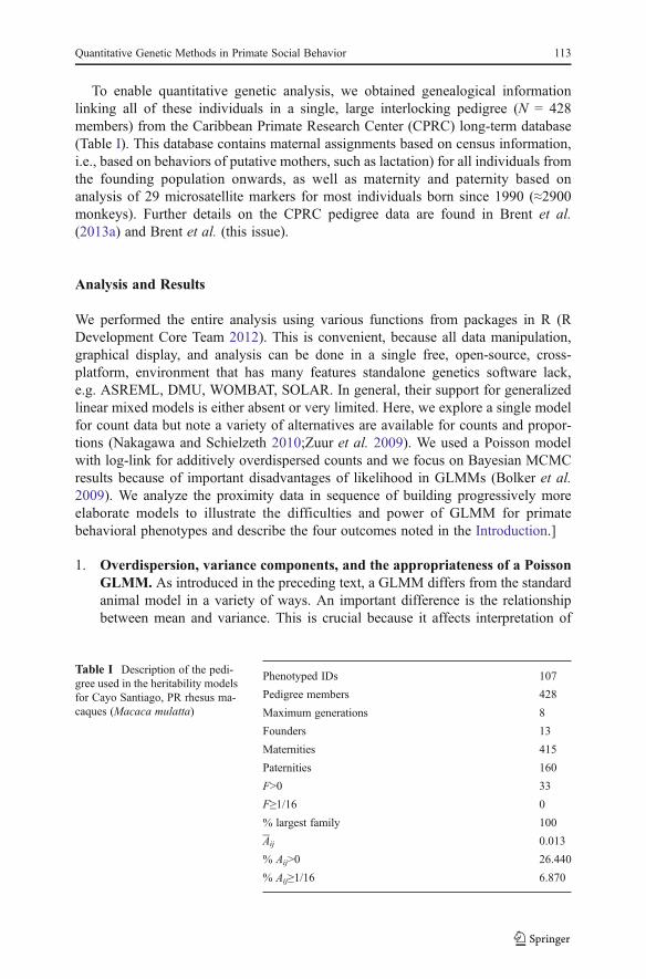
To enable quantitative genetic analysis, we obtained genealogical informationlinking all of these individuals in a single, large interlocking pedigree (N = 428members) from the Caribbean Primate Research Center (CPRC) long-term database(Table I). This database contains maternal assignments based on census information,i.e., based on behaviors of putative mothers, such as lactation) for all individuals fromthe founding population onwards, as well as maternity and paternity based onanalysis of 29 microsatellite markers for most individuals born since 1990 (≈2900monkeys). Further details on the CPRC pedigree data are found in Brent et al.(2013a) and Brent et al. (this issue).

Analysis and Results

We performed the entire analysis using various functions from packages in R (RDevelopment Core Team 2012). This is convenient, because all data manipulation,graphical display, and analysis can be done in a single free, open-source, cross-platform, environment that has many features standalone genetics software lack,e.g. ASREML, DMU, WOMBAT, SOLAR. In general, their support for generalizedlinear mixed models is either absent or very limited. Here, we explore a single modelfor count data but note a variety of alternatives are available for counts and propor-tions (Nakagawa and Schielzeth 2010;Zuur et al. 2009). We used a Poisson modelwith log-link for additively overdispersed counts and we focus on Bayesian MCMCresults because of important disadvantages of likelihood in GLMMs (Bolker et al.2009). We analyze the proximity data in sequence of building progressively moreelaborate models to illustrate the difficulties and power of GLMM for primatebehavioral phenotypes and describe the four outcomes noted in the Introduction.]

1. Overdispersion, variance components, and the appropriateness of a PoissonGLMM. As introduced in the preceding text, a GLMM differs from the standardanimal model in a variety of ways. An important difference is the relationshipbetween mean and variance. This is crucial because it affects interpretation of

Table I Description of the pedi-gree used in the heritability modelsfor Cayo Santiago, PR rhesus ma-caques (Macaca mulatta)

Phenotyped IDs 107

Pedigree members 428

Maximum generations 8

Founders 13

Maternities 415

Paternities 160

F>0 33

F≥1/16 0

% largest family 100

Aij 0.013

% Aij>0 26.440

% Aij≥1/16 6.870


variance components that are used to construct heritabilities. With normallydistributed phenotypes, the mean and variance are separate descriptors of thedistribution. For the animal model with a single additive genetic random effectone could write y~N(Xβ,σa

2 ZAZT+σe2I ) to state that the phenotype has been

treated as a random normal/Gaussian variable with mean X β and varianceσa2Z AZT+σe

2 I. In other words, X β is a vector of fitted values determined bythe fixed effects. The variance components only describe a matrix of covarianceamong the observations in y. For other distributions there may only be a single valuethat controls the entire shape of the distribution. This is true for the Poissondistribution in which the mean and variance are equal (E[y]=λ, the rate parameter).

Using Eq. 2, one would write yePoisson eXβþ∑ni Ziui þ e

� �to state that y is Poisson

distributed with mean and variance equal to eXβþ∑ni Ziui þ e . In this case,

eXβþ∑ni Ziui þ e is a long vector of Poisson rate parameters fit to the observed

data. Observed distributions of count data often have variance > mean, which iscalled overdispersion. A generalized linear mixed model fits heterogeneity in this rateparameter to explain overdispersion through known differences among observationseither through fixed, e.g. sex, age, or random effects, e.g., individual identity in thecase of repeated observations. It is important to note that e is no longer just thedifference between observed and expected values of each observation in y. Instead, itis additional variation in the Poisson rate parameter corresponding to eachobservation in y. The observed values in y are the result of one draw from aPoisson distribution having λ equal to the estimated rate parameter for thatobservation (E[y]). On the link scale, however, the rate parameter is modeled in thesameway as the normal animal model: random effects, and the additive residual e, areassumed to be Gaussian/normal, i.e., this is a Poisson log-normal model.

Overdispersion is a common situation, and it usually indicates there is heteroge-neity among the observations in the underlying biological processes generating thedata. The adult proximity data were overdispersed and did not precisely fit a Poissondistribution (Fig. 1). This is not surprising considering there are many repeatedobservations on each individual; they cover a variety of different demographiccategories of sex, age, and rank; and were collected at different times of the year.The MCMCglmm function from the package of the same name (Hadfield 2010) canbe used in R to fit a GLMM to this data with just an intercept to estimate themean anda single random effect (Elston et al. 2001). This model is E[y]=e1β+e, where eβ is asingle baseline rate parameter common to all observations and e is a vector ofobservation-level random effects that are added to β and adjust the rate parameterfor each observation. A numerical measure of overdispersion is provided by thevariance of this observation-level random effect, σe

2 =0.584. Rather than a singlevalue, MCMC estimates rely on description of a simulated posterior distribution(Gelman and Shirley 2011; Geyer 2011). We retained 1000 samples of posteriordistributions for all models reported. Variance component estimates are taken as theposterior mode. A Bayesian credible interval is also available from the quantiles ofthe posterior distribution. Here, the 95% credible interval for σe

2 was 0.517–0.676,indicating there is a 0.95 probability that the true level of overdispersion falls withinthis interval (Sorensen and Gianola, 2002; Hadfield and Nakagawa, 2010). This level


of overdispersion is small and it declines as other factors are added to the model(Table II). Moreover, a set of graphical checks on the final model explored belowindicate the Poisson assumption is not severely violated (Elston et al., 2001).

If the level of overdispersion were more severe, or the number of zero counts wasmuch larger than expected for a Poisson distribution (zero-inflation), alternatives

0

10

20

30

40

50

0 1 2 3 4 5 6 7 8

number of adults within 2 m

freq

uenc

y

λ = 0.688

Fig. 1 A “rootogram” of the raw proximity data frequencies as grey bars (Wainer, 1974) for CayoSantiago, PR rhesus macaques (Macaca mulatta). Expected frequencies if the counts conformed to aPoisson distribution with the same rate parameter (λ ) are shown with the black line and dots. Bars for theobserved frequencies are shifted up or down to match the Poisson line, making their overlap with thehorizontal axis a simple check on whether the frequency is greater or less than expected. There is an excessat counts ≥3 and at 0, and deficiency at counts 1 and 2.

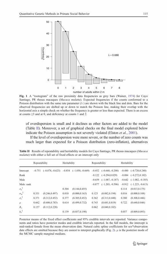
Table II Results of repeatability and heritability models for Cayo Santiago, PR rhesus macaques (Macacamulatta) with either a full set of fixed effects or an intercept only

Repeatability Heritability Repeatability Heritability

Intercept –0.751 (–0.878,–0.623) –0.854 (–1.050,–0.669) –0.452 (–0.660,–0.208) –0.480 (–0.720,0.240)

Rank –0.122 (–0.294,0.029) –0.084 (–0.272,0.102)

Male –0.659 (–1.087,–0.187) –0.642 (–1.082,–0.185)

Male: rank –0.877 (–1.203,–0.596) –0.912 (–1.223,–0.613)

σa2 0.304 (0.144,0.455) 0.114 (0.013,0.175)

σm2 0.351 (0.246,0.497) 0.010 (0.000,0.163) 0.123 (0.082,0.194) 0.016 (0.000,0.108)

σe2 0.371 (0.312,0.452) 0.377 (0.305,0.452) 0.362 (0.313,0.448) 0.380 (0.308,0.446)

μ 0.662 (0.606,0.783) 0.614 (0.499,0.732) 0.743 (0.681,0.819) 0.722 (0.640,0.846)

Ro 0.157 (0.112,0.228) 0.062 (0.040,0.102)

ho2 0.139 (0.057,0.198) 0.057 (0.009,0.093)

Posterior means of the fixed effect coefficients and 95% credible intervals are reported. Variance compo-nents and ratios have posterior modes and credible intervals reported. In the full models, the intercept ismid-ranked female from the mean observation date. Natural cubic spline coefficients for sex*observationdate effects are omitted because they are easiest to interpret graphically (Fig. 2). μ is the posterior mode ofthe MCMC sample marginal medians.


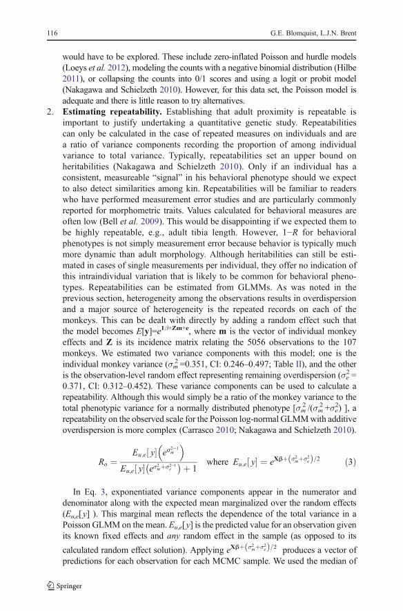
would have to be explored. These include zero-inflated Poisson and hurdle models(Loeys et al. 2012), modeling the counts with a negative binomial distribution (Hilbe2011), or collapsing the counts into 0/1 scores and using a logit or probit model(Nakagawa and Schielzeth 2010). However, for this data set, the Poisson model isadequate and there is little reason to try alternatives.

2. Estimating repeatability. Establishing that adult proximity is repeatable isimportant to justify undertaking a quantitative genetic study. Repeatabilitiescan only be calculated in the case of repeated measures on individuals and area ratio of variance components recording the proportion of among individualvariance to total variance. Typically, repeatabilities set an upper bound onheritabilities (Nakagawa and Schielzeth 2010). Only if an individual has aconsistent, measureable “signal” in his behavioral phenotype should we expectto also detect similarities among kin. Repeatabilities will be familiar to readerswho have performed measurement error studies and are particularly commonlyreported for morphometric traits. Values calculated for behavioral measures areoften low (Bell et al. 2009). This would be disappointing if we expected them tobe highly repeatable, e.g., adult tibia length. However, 1−R for behavioralphenotypes is not simply measurement error because behavior is typically muchmore dynamic than adult morphology. Although heritabilities can still be esti-mated in cases of single measurements per individual, they offer no indication ofthis intraindividual variation that is likely to be common for behavioral pheno-types. Repeatabilities can be estimated from GLMMs. As was noted in theprevious section, heterogeneity among the observations results in overdispersionand a major source of heterogeneity is the repeated records on each of themonkeys. This can be dealt with directly by adding a random effect such thatthe model becomes E[y]=e1β+Zm+e, where m is the vector of individual monkeyeffects and Z is its incidence matrix relating the 5056 observations to the 107monkeys. We estimated two variance components with this model; one is theindividual monkey variance (σm

2 =0.351, CI: 0.246–0.497; Table II), and the otheris the observation-level random effect representing remaining overdispersion (σe

2 =0.371, CI: 0.312–0.452). These variance components can be used to calculate arepeatability. Although this would simply be a ratio of the monkey variance to thetotal phenotypic variance for a normally distributed phenotype [σm

2 /(σm2 +σe

2) ], arepeatability on the observed scale for the Poisson log-normal GLMMwith additiveoverdispersion is more complex (Carrasco 2010; Nakagawa and Schielzeth 2010).

Ro ¼Eu;e y½ � eσ

2�1m

� �Eu;e y½ � eσ2mþσ2−1e

� �þ 1where Eu;e y½ � ¼ eXβþ σ2mþσ2eð Þ=2 ð3Þ

In Eq. 3, exponentiated variance components appear in the numerator anddenominator along with the expected mean marginalized over the random effects(Eu,e[y] ). This marginal mean reflects the dependence of the total variance in aPoisson GLMMon the mean. Eu,e[y] is the predicted value for an observation givenits known fixed effects and any random effect in the sample (as opposed to its

calculated random effect solution). Applying eXβþ σ2mþσ2eð Þ=2 produces a vector ofpredictions for each observation for each MCMC sample. We used the median of


these predictions as the estimate of Eu,e[y] for that sample (Foulley et al. 1987) andthen applied Eq. 3 to it, the fixed effect coefficients, and variance components ineach MCMC sample to generate a posterior distribution of the repeatability.Applying Eq. 3 yields a posterior mode repeatability on the observed count scaleof Ro=0.157 (CI: 0.112–0.228).

There are two other things worth noting about this repeatability. First, it is nottruly comparable to repeatabilities calculated for normally distributed phenotypes inwhich the denominator is the sum of the variance components. For this reason,some authors prefer to call these pseudo-repeatabilities and pseudo-heritabilitiesfrom GLMMs (Foulley et al. 1987; Olesen et al. 1994). Because of the dependenceon the mean and requirement that variance components be positive, the Poissonrepeatability cannot be equal to one. This is common regardless of the link andvariance functions used. Second, a variety of additional information about theindividual monkeys or the observations has been left out of this model.Incorporating these effects is the next task.

3. Adjusting for other effects. The repeatability just described could be upwardly ordownwardly biased by not accounting for other sources of heterogeneity. Upwardbias likely results from not accounting for differences among individuals that areconstant but not necessarily a property of the individual. These are sometimesreferred to as “group level” effects (Nakagawa and Schielzeth 2010). Sex is thebest example of this in the present data set. Males and females have different meanproximity measures. Not accounting for this inflates the mean dissimilarity amongindividuals and the resulting repeatability (Wilson 2008). However, repeated mea-surements on each individual might be taken under very different conditions. Notaccounting for this would depress the repeatability because an individual monkey’smeasurements are more variable than theywould be if it were not for these changingconditions. These are often called “data level” effects. A good example of this hereis seasonal changes in proximity. Each monkey was measured many times oftenweeks or months apart. Any additional factors could enter the GLMM as fixed orrandom effects. The distinction is somewhat arbitrary, but random effects generallyshould only be used when there are many levels sampled, i.e., enough that estimat-ing a variance makes sense, and they are considered to be drawn from a commondistribution (Bolker et al. 2009; McCulloch and Searle 2001). Sex and seasonalityare best modeled as fixed effects. Sex is a simple two-level factor. Seasonal changescould be modeled in a variety of ways. We chose to use natural cubic splines. Theseare local piecewise polynomial fits constrained to be smooth at knot points (Fox2008; Meyer 2005). We used a single knot, placed at the median of days afterJanuary 1, based on visual inspection of the smoothness of the fitted curve and itsoverall correspondence with monthly sex-specific means. Finding seasonal differ-ences between the sexes, we used the interaction between these variables as part ofthe fixed effect model. We also used the interaction of sex and linear effect of socialrank. We standardized rank within sexes and years to fall on a –1 to +1 scale withhighest ranks at –1. Age was the only other variable we tested and found it to havelittle effect on proximity in either sex, with or without the other fixed effects.

To make the intercept more interpretable in our full model, we also mean-centeredobservation date such that it reflected the rate parameter for a female measured on themean day after January 1 (241.2 d≈ September 1) of middle rank (Schielzeth 2010).


In the notation used above, this expanded model is E[y]=eXβ+Zm+e where theadditional fixed effects are reflected in the expanded design matrix X and vector ofcoefficients β.

A common avenue for identifying a suitable set of fixed effects is to run a large setof models and select the best fitting based on information criteria. However, this isoften frowned on by statisticians and we do not advocate it for several reasons(Burnham and Anderson 2002). First, the behavior of information criteria is notwell understood for many GLMMs, potentially making their ranking of modelsunreliable (Spiegelhalter et al. 2002; Wilson et al. 2010). Second, MCMC modelsmust run on the computer for a much longer time to obtain trustworthy results incomparison to traditional likelihood routines for fitting models. Although hardwareimprovements and parallel processing ease this pain, it makes running a large numberof models impractical for most investigators. Finally, no software can substitute forthe careful consideration of the biological questions at hand and limitations ofcollected data to identify suitable models rather than “letting the computer decide.”Along these lines, we would echo the recommendation of Bolker et al. (2009) of along phase of exploratory analysis of graphical displays, descriptive statistics, andmodels with data subsets before attempting to fit a full GLMM.

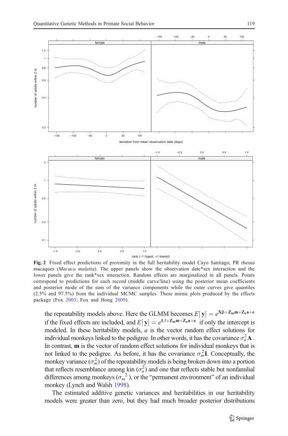
In our case study, the addition of sex*observation date and sex*rank fixedeffects depressed the repeatability of adult proximity, though it clearly remainedgreater than zero (Ro=0.062, CI: 0.040–0.102; Table II, Fig. 3). This wasprimarily because most of the fixed effects are at the “group” level, i.e.,individual monkeys. There is another less obvious difference from theintercept-only repeatability. Along with the changes in variance components,the distributions of Eu,e[y] also differ. This difference is relatively small and isone reason for using the marginal mean (Carrasco 2010). Alternatively, onecould report a range of repeatabilities using different levels of the fixed effects.However, this is unwieldy, because there is a unique repeatability for eachcombination of the fixed effects (Nakagawa and Schielzeth 2010).

Fixed effect coefficients are given on the log scale and should be exponentiatedto interpret them on the original count scale. These are straightforward for theintercept and sex and rank effects (Fig. 3, Table II). For example, the interceptis mid-ranked females (e−0.452=0.636); the coefficient for males is −0.659,which means their mean proximity value is e−0.659=0.517 times the intercept(e−0.452e−0.659=0.329). Spline coefficients are typically explored graphically. Effectplots show a distinct seasonal pattern of a drop in mean proximity in the latesummer corresponding to the beginning of the birth season that is morepersistent for males (Fig. 2, cf. Brent et al. 2013b), and that rank effects aremuch stronger in males. Precision of the fixed and random effect estimates canbe assessed from their credible intervals and these are straightforward to use ingraphical displays.

4. Estimating heritability. Our final step is estimating a heritability of proximity.This is accomplished by the addition of a random effect for individual monkeys thatis linked to the pedigree which allows calculation of an additive genetic variancecomponent that is separate from the monkey variance and overdispersion variancedescribed previously. A corresponding ratio can be constructed for the heritability.For that reason, we have called these heritability models to distinguish them from


the repeatability models above. Here the GLMM becomes E y½ � ¼ eXβþZmmþZaaþe

if the fixed effects are included, and E y½ � ¼ e1βþZmmþZaaþe if only the intercept ismodeled. In these heritability models, a is the vector random effect solutions forindividual monkeys linked to the pedigree. In other words, it has the covariance σa

2A .In contrast,m is the vector of random effect solutions for individual monkeys that isnot linked to the pedigree. As before, it has the covariance σm

2I. Conceptually, themonkey variance (σm

2) of the repeatability models is being broken down into a portionthat reflects resemblance among kin (σa

2) and one that reflects stable but nonfamilialdifferences among monkeys (σm

2 ), or the “permanent environment” of an individualmonkey (Lynch and Walsh 1998).

The estimated additive genetic variances and heritabilities in our heritabilitymodels were greater than zero, but they had much broader posterior distributions

rank (−1 higest, +1 lowest)

num

ber

of a

dults

with

in 2

m

0.1

0.2

0.5

1

2

−1.0 −0.5 0.0 0.5 1.0

female

−1.0 −0.5 0.0 0.5 1.0

male

deviation from mean observation date (days)

num

ber

of a

dults

with

in 2

m

0.2

0.4

0.6

0.8

1

1.2

−150 −100 −50 0 50 100

female

−150 −100 −50 0 50 100

male

Fig. 2 Fixed effect predictions of proximity in the full heritability model Cayo Santiago, PR rhesusmacaques (Macaca mulatta). The upper panels show the observation date*sex interaction and thelower panels give the rank*sex interaction. Random effects are marginalized in all panels. Pointscorrespond to predictions for each record (middle curve/line) using the posterior mean coefficientsand posterior mode of the sum of the variance components while the outer curves give quantiles(2.5% and 97.5%) from the individual MCMC samples. These mimic plots produced by the effectspackage (Fox 2003; Fox and Hong 2009).


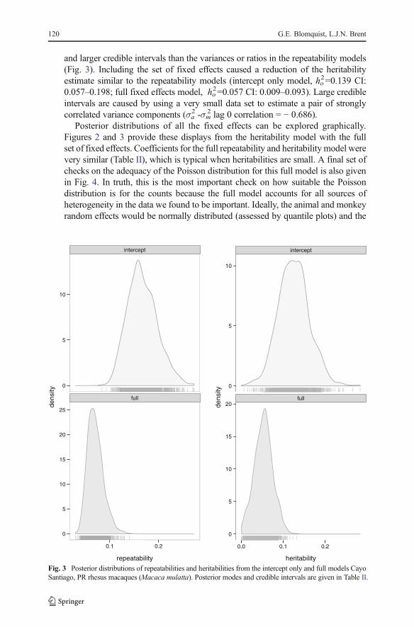
and larger credible intervals than the variances or ratios in the repeatability models(Fig. 3). Including the set of fixed effects caused a reduction of the heritabilityestimate similar to the repeatability models (intercept only model, ho

2=0.139 CI:0.057–0.198; full fixed effects model, ho

2=0.057 CI: 0.009–0.093). Large credibleintervals are caused by using a very small data set to estimate a pair of stronglycorrelated variance components (σa

2 -σm2 lag 0 correlation = − 0.686).

Posterior distributions of all the fixed effects can be explored graphically.Figures 2 and 3 provide these displays from the heritability model with the fullset of fixed effects. Coefficients for the full repeatability and heritability model werevery similar (Table II), which is typical when heritabilities are small. A final set ofchecks on the adequacy of the Poisson distribution for this full model is also givenin Fig. 4. In truth, this is the most important check on how suitable the Poissondistribution is for the counts because the full model accounts for all sources ofheterogeneity in the data we found to be important. Ideally, the animal and monkeyrandom effects would be normally distributed (assessed by quantile plots) and the

intercept

full

0

5

10

0

5

10

15

20

25

0.1 0.2

repeatability

dens

ity

intercept

full

0

5

10

0

5

10

15

20

0.0 0.1 0.2

heritability

dens

ity

Fig. 3 Posterior distributions of repeatabilities and heritabilities from the intercept only and full models CayoSantiago, PR rhesus macaques (Macaca mulatta). Posterior modes and credible intervals are given in Table II.


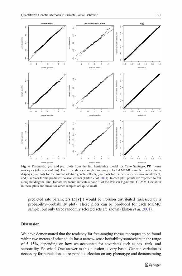
predicted rate parameters (E[y] ) would be Poisson distributed (assessed by aprobability–probability plot). These plots can be produced for each MCMCsample, but only three randomly selected sets are shown (Elston et al. 2001).

Discussion

We have demonstrated that the tendency for free-ranging rhesus macaques to be foundwithin two meters of other adults has a narrow-sense heritability somewhere in the rangeof 5–15%, depending on how we accounted for covariates such as sex, rank, andseasonality. So what? One answer to this question is very basic. Genetic variation isnecessary for populations to respond to selection on any phenotype and demonstrating

−3 −2 −1 0 1 2 3

−1.

0−

0.5

0.0

0.5

1.0

animal effect

normal quantiles

sam

ple

quan

tiles

−2 −1 0 1 2

−0.

4−

0.2

0.0

0.2

0.4

permanent env. effect

normal quantilessa

mpl

e qu

antil

es

0.0 0.2 0.4 0.6 0.8 1.0

0.0

0.2

0.4

0.6

0.8

1.0

E[y]

scaled rank

Poi

sson

cum

ulat

ive

dist

ribut

ion

−3 −2 −1 0 1 2 3

−0.

50.

00.

5

normal quantiles

sam

ple

quan

tiles

−2 −1 0 1 2

−1.

0−

0.5

0.0

0.5

normal quantiles

sam

ple

quan

tiles

0.0 0.2 0.4 0.6 0.8 1.0

0.0

0.2

0.4

0.6

0.8

1.0

scaled rankP

oiss

on c

umul

ativ

e di

strib

utio

n

−3 −2 −1 0 1 2 3

−0.

50.

00.

51.

0

normal quantiles

sam

ple

quan

tiles

−2 −1 0 1 2

−0.

4−

0.2

0.0

0.2

0.4

0.6

normal quantiles

sam

ple

quan

tiles

0.0 0.2 0.4 0.6 0.8 1.0

0.0

0.2

0.4

0.6

0.8

1.0

scaled rank

Poi

sson

cum

ulat

ive

dist

ribut

ion

Fig. 4 Diagnostic q–q and p–p plots from the full heritability model for Cayo Santiago, PR rhesusmacaques (Macaca mulatta). Each row shows a single randomly selected MCMC sample. Each columndisplays q–q plots for the animal additive genetic effects, q–q plots for the permanent environment effect,and p–p plots for the predicted Poisson counts (Elston et al. 2001). In each plot, points are expected to fallalong the diagonal line. Departures would indicate a poor fit of the Poisson log-normal GLMM. Deviationin these plots and those for other samples are quite small.


that there is a genetic basis to primate behavior is therefore an important first step indescribing its potential evolutionary trajectory. Although behavioral measurements havebeen included in heritability estimates for multivariable abstractions such as socialnetwork statistics (Brent et al. 2013a), and behavioral tendencies (Williamson et al.2003; Adams et al. 2012; Brent et al. .this issue) to our knowledge, this is the firstdemonstration that tendency for adult primates to be in proximity with one another isheritable. The increased availability of pedigrees and power of animal model methodsmay change this in the near future. However, there is much more that can and should bedone with quantitative genetic models and methods.

Before exploring useful applications of a heritability estimate and extensions, it is worthrecalling some of the pitfalls of interpretation. These are well known and have beendiscussed by many authors but are worth recounting (Adams 2011; Roff 1997; Vitzthum2003; Visscher et al. 2008). First, high heritabilities should not always be expected forphenotypes where genes are thought to play an important role. Heritabilities are fractions ofphenotypic variance. Many traits that undoubtedly require interacting networks of genes,e.g. the presence of a brain in adults, do not vary and therefore have undefined heritabilities.Moreover, because heritabilities are dependent on allele frequencies and environmentalconditions in a population, a large heritability could be the result of small environmentalvariance (Charmantier andGarant 2005). Animalmodel heritabilities are also dependent onhow the phenotypic variance is calculated. If fixed effects primarily affect the phenotypicvariance, then removal of their variance from the denominator of the heritability will resultin higher heritabilities (Wilson 2008). GLMM “pseudo-heritabilities” may also haveadditional quirks such as the dependence on the overall mean in the Poisson case exploredin the preceding text. Second, a low heritability does not mean genes play no role inshaping phenotypic variance. Again, because heritabilities are ratios, a low value couldresult from large environmental variance even when additive genetic variance is greaterthan zero. Price and Schluter (1991) argue this is likely a common situation for behavioraland life history traits that are contingent on other physiological and social circumstances.Finally, heritabilities describe intrapopulation variation. Therefore, a simple heritabilityestimate is next to useless for describing intergroup differences. For example, the differencein mean proximity between monkeys in group F and those in any other social groupprobably have nothing to do with genetics, and a heritability estimate of 5% certainlywould not mean that 5% of any mean difference in proximity between groups is due to theadditive effect of genes (Brommer 2011).

Avoiding these pitfalls, we would highlight some appropriate uses of heritabilityestimates and areas for extension. First, heritabilities link very directly to simplequantitative models of evolutionary change, such as response to directional selectionin the breeder’s equation (R=h2S ; Roff 1994, 1997). In this equation, intergenerationalchange in the mean (R =response) is always a fraction of the selection differential (S )equal to h2. A small heritability such as the one estimated for adult proximity impliesvery slow response to selection. This is typical of behavioral phenotypes which oftenhave lower heritabilities than morphological traits (cf. Stirling et al. 2002). The responseto directional selection of phenotypes with non-normal distributions, such as Poissoncounts, is somewhat different because of the mean–variance equality but it has beenmodeled (Korsgaard et al. 2002).

Second, heritability estimates are often an effective tool for initial screening ofphenotypes amenable to exploring the molecular signatures of inheritance through


genome-wide association (GWAS) and or linkage mapping (Visscher et al. 2010).Once identified, loci can be subjected to a variety of tests for departures fromequilibrium including molecular signatures of selection. Well-characterized loci fromlaboratory settings that have documented associations with behavioral patterns canalso be incorporated, e.g., neurotransmitter production and regulation; Brent et al.2013a). These are enticing research projects that are treated in great detail by otherauthors and emphasize the “genetic” side of quantitative genetics (Bradley andLawler 2011;Tung et al. 2010). The allure of molecular genetics need not overshadowthe advantages of quantitative genetic techniques themselves.

Instead of fretting over the molecular details of inheritance, we should alsoconsider quantitative genetic methods relevant for addressing the equally excitingcomplexity of environments primates experience and construct for each other.Lengthy developmental periods in primates have often been argued to be opportuni-ties for parental and peer effects on behavioral phenotypes (Leigh 2001; Maestripieri2009). There are sophisticated quantitative genetic models for describing such effectsthrough variance components or covariances between social partner phenotypes andthey often have very different dynamics from the intuitive breeder’s equation(Cheverud and Wolf 2009; Moore et al. 2002; Adams, this issue). Moreover, theflexibility of primate behavior and depth of longitudinal measurements on knownindividuals are an opportunity for studying the evolution and genetics of plasticity.Plasticity itself can be treated as a phenotype (Schlichting and Pigliucci 1998) whenindividuals are measured across environmental gradients and individual reactionnorms can be calculated (Dingemanse and Dochtermann 2013; Dingemanse et al.2010; Martin et al. 2011). For example, in our case study we treated spatial associ-ation as the same trait regardless of season of measurement. In other words, ifproximity in the birth and nonbirth seasons were, in fact, two different traits our casestudy analysis requires we assume the genetic correlation between these traits is 1 andtheir heritabilities are equal. It is an open question as to how realistic these assump-tions are. Given large enough data sets, they can be tested with multivariate andrandom regression quantitative genetic models (Brommer et al. 2012).

Power concerns will often limit the applicability and complexity of quantitativegenetic models for unmanaged primate populations. The number of such populationswith well-resolved pedigrees is rapidly increasing, thus removing the other major barrierto the application of quantitative genetics to studies of primate behavior. We wouldencourage primatologists wishing to employ these techniques to use simulations on theirpedigrees to identify the necessary number of individuals to measure to achievesufficient power, e.g., for detecting nonzero genetic variance). For example, Quinnet al. (2006) showed a total of 300 measured individuals was sufficient to generateprecise estimates of heritabilities and genetic correlations in two bird populations.Although this figure is currently unattainable for most any primate behavioral study,our analysis of spatial association used considerably fewer individuals, but was still ableto detect a nonzero genetic variance. Because of the strong influence of pedigreestructure, the locations of measured individuals within the pedigree, measurement error,and how well environmental effects are accounted for, there is no clear “rule of thumb”to guide when quantitative genetic analysis is or is not worthwhile. However, we wouldsuggest samples<100 are unlikely to be of much use. This places a considerable limit onthe current applicability of quantitative genetics to all but the longest-running primate


field sites, and may preclude such analysis with understudied and endangered species.Nevertheless, large-scale sampling efforts are currently underway at a number of fieldsites, and would be feasible to implement over relatively short periods of time at others.We therefore encourage primatologists in the future to consider the requirements ofquantitative genetic techniques when designing data collection protocols.

We close by noting an indirect but potentially far-reaching contribution of quan-titative genetics by wondering, should behavioral ecology become like comparativebiology? Hardly any interspecific comparative study is published today that does notsomehow account for the phylogenetic relationships among study species (Freckleton2009; Housworth et al. 2004). Primate behavioral ecologists face a similar problem ofnon-independence among the individual members of the populations they studybecause many primate groups consist of sets of kin, and kin may not be randomizedacross environments (Blomquist 2009a; Silk 1984). In comparative studies thephylogenetic history of species is most influential for identifying interspecific pat-terns, e.g., evolutionary allometries, when those patterns are weak (Klingenberg1996). Because ecological trends are typically quite weak (Nee et al. 2005;Peters1991), the genealogy of primate groups could make a huge difference for establishinghow population members respond to changing social and climatic conditions that arethe foundation of primate theoretical and field ecology (Campbell et al. 2011;Clutton-Brock and Janson 2012). The increasing availability of pedigrees, or tech-niques to construct them, for wild primates begs for deeper appreciation and directtreatment of this problem. Just as comparative biologists use a phylogeny as a tool foranalysis of interspecific data without any direct interest in discovering phylogeny,perhaps ecologists should be using pedigrees even when they are uninterested ingenealogy or estimating heritabilities.

Acknowledgments We thank the Caribbean Primate Research Center (CPRC) for the permission toundertake research on Cayo Santiago, along with Bonn Aure and Jacqueline Buhl, who assisted in datacollection, and Elizabeth Maldonado, Angelina Ruiz-Lambides, and Janis Gonzalez-Martinez, who pro-vided access to the CPRC pedigree database. L. J. N. Brent also thanks Michael Platt for mentorship duringthe collection of these data. L. J. N. Brent was funded by fellowships awarded by the Duke Center forInterdisciplinary Decision Sciences. Additional funds were provided by NIMH grants no. R01-MH096875and R01-MH089484. The CPRC is supported by a grant no. 8-P40 OD012217-25 from the National Centerfor Research Resources (NCRR) and the Office of Research Infrastructure Programs (ORIP) of the NationalInstitutes of Health. G. E. Blomquist is supported by the University of Missouri Department of Anthro-pology and Research Council. G. E. Blomquist also thanks L. J. N. Brent and Noah Snyder-Mackler for theinvitation to participate in the International Primatological Society symposium leading to this special issue.

References

Adams, M. J. (2011). Evolutionary genetics of personality in nonhuman primates. In M. Inoue-Murayama,S. Kawamura, & A. Weiss (Eds.), From genes to animal behavior (pp. 137–164). New York: Springer.

Adams, M. J., King, J. E., & Weiss, A. (2012). The majority of genetic variation in orangutan personalityand subjective well-being is nonadditive. Behavior Genetics, 42, 675–686.

Arnold, S. J. (1994). Multivariate inheritance and evolution: A review of concepts. In C. R. B. Boake (Ed.),Quantitative genetic studies of behavioral evolution (pp. 17–48). Chicago: University of Chicago Press.

Bell, A. M., Hankison, S. J., & Laskowski, K. L. (2009). The repeatability of behaviour: A meta-analysis.Animal Behaviour, 77(4), 771–783.


Bennett, A. J., & Pierre, P. J. (2010). Nonhuman primate research contributions to understanding geneticand environmental influences on phenotypic outcomes across development. In K. E. Hood, C. T.Halpern, G. Greenberg, & R. M. Lerner (Eds.), Handbook of developmental science, behavior, andgenetics (pp. 353–399). New York: Blackwell.

Blomquist, G. E. (2009a). Environmental and genetic causes of maturational differences among rhesusmacaque matrilines. Behavioral Ecology and Sociobiology, 63(9), 1345–1352.

Blomquist, G. E. (2009b). Fitness-related patterns of genetic variation in rhesus macaques. Genetica, 135,209–219.

Boake, C. R. B. (1994). Quantitative genetic studies of behavioral evolution. Chicago: University ofChicago Press.

Boake, C. R. B., Arnold, S. J., Breden, F., Meffert, L. M., Ritchie, M. G., Taylor, B. J., Wolf, J. B., &Moore, A. J. (2002). Genetic tools for studying adaptation and the evolution of behavior. AmericanNaturalist, 160, S143–S159.

Bolker, B. M., Brooks, M. E., Clark, C. J., Geange, S. W., Poulsen, J. R., Stevens, M. H. H., Simone, S., &White, J. (2009). Generalized linear mixed models: A practical guide for ecology and evolution. Trendsin Ecology and Evolution, 24(3), 127–135.

Bradley, B. J., & Lawler, R. R. (2011). Linking genotypes, phenotypes, and fitness in wild primatepopulations. Evolutionary Anthropology, 20(3), 104–119.

Brent, L. J. N., Heilbronner, S. R., Horvath, J. E., Gonzalez-Martinez, J., Ruiz-Lambides, A., Robinson, A.G., Skene, J. H. P., & Platt, M. L. (2013a). Genetic origins of social networks in rhesus macaques.Scientific Reports, 3, 1042.

Brent, L. J. N., MacLarnon, A., Platt, M. L., & Semple, S. (2013b). Seasonal changes in the structure ofrhesus macaque social networks. Behavioral Ecology and Sociobiology, 67, 349–359.

Brommer, J. E. (2011). Whither PST ? the approximation of QST by PST in evolutionary and conservationbiology. Journal of Evolutionary Biology, 24, 1160–1168.

Brommer, J. E., Kontiainen, P., & Pietiäinen, H. (2012). Selection on plasticity of seasonal life-history traitsusing random regression mixed model analysis. Ecology and Evolution, 2, 695–704.

Burnham, K. P., & Anderson, D. R. (2002). Model selection and multimodel inference: A practicalinformation-theoretic approach (2nd ed.). New York: Springer.

Campbell, C. J., Fuentes, A., MacKinnon, K. C., Bearder, S., & Stumpf, R. (Eds.). (2011). Primates inperspective. New York: Oxford University Press.

Carrasco, J. L. (2010). A generalized concordance correlation coefficient based on the variance componentsgeneralized linear mixed models for overdispersed count data. Biometrics, 66, 897–904.

Charmantier, A., & Garant, D. (2005). Environmental quality and evolutionary potential: Lessons fromwild populations. Proceedings of the Royal Society of London B: Biological Sciences, 272, 1415–1425.

Cheverud, J. M., & Dittus, W. P. J. (1992). Primate population studies at Polonnaruwa II. Heritability ofbody measurements in a natural population of toque macaques. American Journal of Primatology, 27,145–156.

Cheverud, J. M., & Moore, A. J. (1994). Quantitative genetics and the role of the environment provided byrelatives in behavioral evolution. In C. R. B. Boake (Ed.), Quantitative genetic studies of behavioralevolution (pp. 67–100). Chicago: University of Chicago Press.

Cheverud, J. M., & Wolf, J. B. (2009). The genetics and evolutionary consequences of maternal effects. InD. Maestripieri & J. M. Mateo (Eds.), Maternal effects in mammals (pp. 11–37). Chicago: Universityof Chicago Press.

Clutton-Brock, T., & Janson, C. (2012). Primate socioecology at the crossroads: Past, present, and future.Evolutionary Anthropology, 21, 136–150.

Dingemanse, N. J., & Dochtermann, N. A. (2013). Quantifying individual variation in behaviour: Mixed-effect modelling approaches. Journal of Animal Ecology, 82, 39–54.

Dingemanse, N. J., Kazem, A. J. N., Réale, D., & Wright, J. (2010). Behavioural reaction norms: Animalpersonality meets individual plasticity. Trends in Ecology and Evolution, 25, 81–89.

Dingemanse, N. J., & Réale, D. (2005). Natural selection and animal personality. Behaviour, 142, 1165–1190.Elston, D. A., Moss, R., Boulinier, T., Arrowsmith, C., & Lambin, X. (2001). Analysis of aggregation, a

worked example: Numbers of ticks on red grouse chicks. Parasitology, 122, 563–569.Foulley, J. L., Gianola, D., & Im, S. (1987). Genetic evaluation of traits distributed as poisson-binomial

with reference to reproductive characters. Theoretical and Applied Genetics, 73, 870–877.Fox, J. (2003). Effect displays in R for generalised linear models. Journal of Statistical Software, 8(15), 1–27.Fox, J. (2008). Applied regression analysis and generalized linear models (2nd ed.). Thousand Oaks, CA: SAGE.


Fox, J., & Hong, J. (2009). Effect displays in R for multinomial and proportional-odds logit models:Extensions to the effects package. Journal of Statistical Software, 32(1), 1–24.Available at: http://www.jstatsoft.org/v32/i01/

Freckleton, R. P. (2009). The seven deadly sins of comparative analysis. Journal of Evolutionary Biology,22(7), 1367–1375.

Frentiu, F. D., Clegg, S. M., Chittock, J., Burke, T., Blows, M. W., & Owens, I. P. F. (2008). Pedigree-freeanimal models: The relatedness matrix reloaded. Proceedings of the Royal Society of London B:Biological Sciences, 275, 639–647.

Gelman, A., & Shirley, K. (2011). Inference from simulations and monitoring convergence. InS. Brooks,Gelman A, Jones GL, Meng X (eds) Handbook of Markov Chain Monte Carlo, CRC Press, London,chap 6, pp 163–174

Geyer, C. J. (2011). Introduction to Markov chain Monte Carlo. In S. Brooks, A. Gelman, G. L. Jones, & X.Meng (Eds.), Handbook of Markov Chain Monte Carlo (pp. 3–48). London: CRC Press.

Grafen, A. (1984). Natural selection, kin selection and group selection. In J. R. Krebs & N. B. Davies(Eds.), Behavioural ecology: An evolutionary approach (2nd ed., pp. 62–84). New York: Blackwell.

Hadfield, J. D. (2010). MCMC methods for multi-response generalized linear mixed models: TheMCMCglmm R package. Journal of Statistical Software, 33(2), 1–22.

Hadfield, J. D., & Nakagawa, S. (2010). General quantitative genetic methods for comparative biology:Phylogenies, taxonomies and multi-trait models for continuous and categorical characters. Journal ofEvolutionary Biology, 23(3), 494–508.

Hadfield, J. D., Nutall, A., Osorio, D., & Owens, I. P. (2007). Testing the phenotypic gambit: Phenotypic,genetic and environmental correlations of colour. Journal of Evolutionary Biology, 20, 549–557.

Hilbe, J. M. (2011). Negative binomial regression (2nd ed.). New York: Cambridge University Press.Housworth, E. A., Martins, E. P., & Lynch, M. (2004). The phylogenetic mixed model. American

Naturalist, 163(1), 84–96.Jones, C. B. (2005). Behavioral flexibility in primates: Causes and consequences. New York: Springer.Klingenberg, C. P. (1996). Multivariate allometry. In L. F. Marcus, M. Corti, A. Loy, G. J. P. Naylor, & D.

E. Slice (Eds.), Advances in morphometrics (pp. 23–49). New York: Plenum Press.Korsgaard, I. R., Andersen, A. H., & Jensen, J. (2002). Prediction error variance and expected response to

selection, when selection is based on the best predictor—for Gaussian and threshold characters, traitsfollowing a Poisson mixed model and survival traits. Genetics, Selection, Evolution, 34, 307–333.

Kruschke, J. (2011). Doing Bayesian data analysis: A tutorial introduction with R and BUGS. Burlington,MA: Academic Press.

Kruuk, L. E. B. (2004). Estimating genetic parameters in natural populations using the ‘animal model.Philosophical Transactions of the Royal Society of London B: Biological Sciences, 359(1446), 873–890.

Kruuk, L. E. B., Slate, J., & Wilson, A. J. (2008). New answers for old questions: The evolutionaryquantitative genetics of wild animal populations. Ecology, 39, 525–548.

Lande, R. (1982). A quantitative genetic theory of life history evolution. Ecology, 63(3), 607–615.Lawler, R. R. (2006). Sifaka positional behavior: Ontogenetic and quantitative genetic approaches.

American Journal of Physical Anthropology, 131, 261–271.Leigh, S. R. (2001). Evolution of human growth. Evolutionary Anthropology, 10, 223–236.Loeys, T., Moerkerke, B., De Smet, O., & Buysse, A. (2012). The analysis of zero-inflated count data: Beyond

zero-inflated Poisson regression. British Journal of Mathematical and Statistical Psychology, 65, 163–180.Lynch,M., &Walsh, B. (1998).Genetics and analysis of quantitative traits. Sunderland,MA: Sinauer Associates.Maestripieri, D. (2009). Maternal influences on offspring growth, reproduction, and behavior in primates.

In D. Maestripieri & J. M. Mateo (Eds.), Maternal effects in mammals (pp. 256–291). Chicago:University of Chicago Press.

Martin, J. G. A., Nussey, D. H., Wilson, A. J., & Réale, D. (2011). Measuring individual differences inreaction norms in field and experimental studies: A power analysis of random regression models.Methods in Ecology and Evolution, 2, 362–374.

McCulloch, C. E., & Searle, S. R. (2001).Generalized, linear, and mixed models. NewYork: JohnWiley & Sons.Meyer, K. (2005). Random regression analyses using B-splines to model growth of Australian Angus cattle.

Genetics, Selection, Evolution, 37, 473–500.Moore, A. J., Haynes, K. F., Preziosi, R. F., & Moore, P. J. (2002). The evolution of interacting phenotypes:

Genetics and evolution of social dominance. American Naturalist, 160, S186–S197.Morrissey, M. B., & Wilson, A. J. (2010). pedantics: An r package for pedigree-based genetic simulation

and pedigree manipulation, characterization and viewing. Molecular Ecology Resources, 10, 711–719.


http://www.jstatsoft.org/v32/i01/

http://www.jstatsoft.org/v32/i01/

Nakagawa, S., & Schielzeth, H. (2010). Repeatability for Gaussian and non-Gaussian data: A practicalguide for biologists. Biological Reviews of the Cambridge Philosophical Society, 85, 935–956.

Nee, S., Colegrave, N., West, S. A., & Grafen, A. (2005). The illusion of invariant quantities in lifehistories. Science, 309, 1236–1239.

O’Hara, R. B., Cano, J. M., Ovaskainen, O., Teplitsky, C., & Ahlo, J. S. (2008). Bayesian approaches inevolutionary quantitative genetics. Journal of Evolutionary Biology, 21, 949–957.

Olesen, I., Perez-Enciso, M., Gianola, D., & Thomas, D. L. (1994). A comparison of normal andnonnormal mixed models for number of lambs born in Norwegian sheep. Journal of AnimalScience, 72, 1166–1173.

Pemberton, J. M. (2008). Wild pedigrees: The way forward. Proceedings of the Royal Society of London B:Biological Sciences, 275, 613–621.

Peters, R. H. (1991). A critique for ecology. New York: Cambridge University Press.Plomin, R., DeFries, J. C., McClearn, G. E., & McGuffin, P. (2009). Behavioral genetics (5th ed.). New

York: Worth.Price, T., & Schluter, D. (1991). On the low heritability of life history traits. Evolution, 45, 853–861.Quinn, J. L., Charmantier, A., Garant, D., & Sheldon, B. C. (2006). Data depth, data completeness, and

their influence on quantitative genetic estimation in two contrasting bird populations. Journal ofEvolutionary Biology, 19, 994–1002.

R Development Core Team. (2012). R: A language and environment for statistical computing. Vienna,Austria: R Foundation for Statistical Computing. Available at: http://www.R-project.org

Rawlins, R. G., & Kessler, M. J. (Eds.). (1986). The Cayo Santiago macaques: History, behavior, andbiology. Albany: SUNY Press.

Roff, D. A. (1994). Optimality modeling and quantitative genetics: A comparison of the two approaches. InC. R. B. Boake (Ed.), Quantitative genetic studies of behavioral evolution (pp. 49–66). Chicago:University of Chicago Press.

Roff, D. A. (1997). Evolutionary quantitative genetics. New York: Chapman and Hall.Schielzeth, H. (2010). Simple means to improve the interpretability of regression coefficients. Methods in

Ecology and Evolution, 1, 103–113.Schlichting, C. D., & Pigliucci, M. (1998). Phenotypic evolution: A reaction norm perspective. Sunderland,

MA: Sinauer Associates.Silk, J. B. (1984). Measurement of the relative importance of individual selection and kin selection among

females of the genus Macaca. Evolution, 38(3), 553–559.Silk, J. B. (2002). Using the “f”-word in primatology. Behaviour, 139, 421–446.Sillanpää, M. J. (2011). On statistical methods for estimating heritability in wild populations. Molecular

Ecology, 20(7), 1324–1332.Sorensen, D., & Gianola, D. (2002). Likelihood, Bayesian, and MCMC methods in quantitative genetics.

New York: Springer.Spencer, H. G. (2009). Effects of genomic imprinting on quantitative traits. Genetica, 136, 285–293.Spiegelhalter, D. J., Best, N. G., Carlin, B. P., & Van Der Linde, A. (2002). Bayesian measures of model

complexity and fit. Journal of the Royal Statistical Society B: Statistical Methodology, 64, 583–639.Stirling, D. G., Reale, D., & Roff, D. A. (2002). Selection, structure and the heritability of behaviour.

Journal of Evolutionary Biology, 15, 277–289.Tung, J., Alberts, S. C., & Wray, G. A. (2010). Evolutionary genetics in wild primates: Combining genetic

approaches with field studies of natural populations. Trends in Genetics, 26, 353–362.van Oers, K., & Sinn, D. L. (2011). Toward a basis for the phenotypic gambit: Advances in the evolutionary

genetics of animal personality. In M. Inoue-Murayama, S. Kawamura, & A. Weiss (Eds.), From genesto animal behavior (pp. 165–183). New York: Springer.

Visscher, P. M., Hill, W. G., & Wray, N. R. (2008). Heritability in the genomics era—concepts andmisconceptions. Nature Reviews Genetics, 9, 255–266.

Visscher, P. M., McEvoy, B., & Yang, J. (2010). From Galton to GWAS: Quantitative genetics of humanheight. Genetical Research, 92, 371–379.

Vitzthum, V. J. (2003). A number no greater than the sum of its parts: The use and abuse of heritability.Human Biology, 75, 539–558.

Wainer, H. (1974). The suspended rootogram and other visual displays: An empirical validation. AmericanStatistician, 28, 143–145.

Weiss, A., King, J. E., & Enns, R. M. (2002). Subjective well-being is heritable and genetically correlatedwith dominance in chimpanzees (Pan troglodytes). Journal of Personality and Social Psychology,83(5), 1141–1149.


http://www.R-project.org

Williamson, D. E., Coleman, K., Bacanu, S., Devlin, B. J., Rogers, J., Ryan, N. D., & Cameron, J. L.(2003). Heritability of fearful-anxious endophenotypes in infant rhesus macaques: A preliminaryreport. Biological Psychiatry, 53, 284–291.

Wilson, A. J. (2008). Why h2 does not always equal VA/VP ? Journal of Evolutionary Biology, 21(3), 647–650.Wilson, A. J., Reale, D., Clements, M. N., Morrissey, M. M., Postma, E., Walling, C. A., Kruuk, L. E. B., &

Nussey, D. H. (2010). An ecologist’s guide to the animal model. Journal of Animal Ecology, 79, 13–26.Zuur, A., Ieno, E. N., Walker, N., Saveliev, A. A., & Smith, G. M. (2009). Mixed effects models and

extensions in ecology with R. New York:Springer.


Documents

Applying Quantitative Genetic Methods to Primate Social Behavior · 2020-02-17 · In contrast, primate behavioral ecology has typically lacked a quantitative genetic dimension in