Embed Size (px)
Citation preview

American Research Journal of Mechanical and Automation Engineering Original Article
Volume 1, Issue1, 2015
www.arjonline.org 1
Applying Quantum Interference in UAVs to Provide Smart
Geophysical Mineral Exploration and Exploitation
Aakash Gupta
Department of Aerospace and Mechanical Engineering,
Parks College of Engineering, Aviation, and Technology
Saint Louis University
Abstract: Due to high metal and petroleum prices and increased difficulties in finding shallower deposits, the
exploration for and exploitation of mineral resources is expected to move to greater depths. Consequently,
seismic methods will become a more important tool to help unravel structures hosting mineral deposits at great
depth for mine planning and exploration. These methods also can be used with varying degrees of success to directly target mineral deposits at depth.
Quantum interference is a principle of quantum mechanics that deals with analyzing particle-wave nature sub-
atomic particles, especially concepts like photon interference and duality of light. This theoretical concept has
aided in practically determining solutions for materials of superconductivity, “they have simulated a working
molecular thermoelectric material capable of turning heat into electricity”.4 Furthermore, quantum mechanics
provides highly precise efficiency and accuracy in measuring and analyzing techniques.
Designing the Unmanned Airborne Vehicle (UAVs) equipped with the applications of quantum interference can
help us achieve precise data and measurements for navigation and seismic studies. Currently, seismic ships are
into practical usage for gathering data, which are then transferred from the collection unit to the processing center
and gets manipulated into 3D designs for detailed analysis. However, a quantum UAV can posses a capability to
gather data more precisely and at a relatively higher precision rate in comparison to seismic ships. Quantum computing in an UAV will enable real time processing of seismic and navigational data into 3D models for
analysis.
I. INTRODUCTION
Unmanned Airborne Vehicles are pilot-less aircraft that are flown on military, commercial, and police missions for a
variety of applications. They are gaining in popularity, as they are inexpensive, collect good quality data from a
stable platform, and they can be equipped with many kinds of sensors, ranging from simple cameras to infrared
cameras to magnetometers. Driven initially by military applications, platforms, such as helicopter and fixed wing,
have evolved significantly in the past ten years with new technology improvements, efficiency, range, size and
payload of UAVs. While these developments have been outside the commercial sector, this trend is changing, as
more and more commercial applications are uncovered.
The primary commercial use to date has been in mineral exploration but the other fields are developing. Mineral
exploration is a natural fit for a UAV for a number of reasons. Manned flights in remote areas are dangerous and
cost significant resources to support, including mechanics, fuel dumps, and more. UAVs are easier to launch,
mobilize, set up and refuel. Moreover, UAVs can fly in all weather and at night – giving significant productivity
gains over conventional airborne surveys.
Mineral exploration under the waterbed has been performed by ships and has been left aloof for UAVs until now.
This research has focused on solving that matter with the usage of UAVs that can explore the water bodies for
mineral exploration at a much faster and efficient way through a highly equipped sensor technology incorporated in
a UAV plan design.
II. ADVANTAGES OF UAVS
The UA can fly day-after-day, night-after-night, in dangerous weather conditions, for up to 30 hours at a time, on
an accurate flight path, under computer control.
Since Unmanned Aircraft can follow a precise flight path, they can fly close to each other to complete a survey
in far less time than would be required for a manned aircraft.

American Research Journal of Mechanical and Automation Engineering, Volume 1, Issue 1, 2015
www.arjonline.org 2
An advantage in using several Unmanned Aircraft is that an UA that develops a fault in any of its systems can be
replaced by a back-up UA, ensuring the assigned task is always completed on time. Several Unmanned Aircraft
can also measure data in the same location in a survey, to provide quality data, by removing any instrument drift
or errors.
It can fly safely at low altitudes, enabling high resolution aeromagnetic mapping.
Network Centric approach in which data from each UA in flight updates a server computer in real time, allowing users to view the latest information, via the Internet.
It costs less to buy, to fly, to operate, to land and to dispose of than a piloted plane
The UA is more environmentally friendly: it is small, uses less fuel, creates less CO 2 and is less noisy: 16 g/km
fuel for a UA vs 152 g/km for a Cessna Skylane.
III. METHODOLOGY
Types of UAV technology that has to be taken into consideration include Volume Surveys, Digital Terrain Models,
and Counter Mapping. This can be achieved by the following:
Sensor fusion: Combining information from different sensors for use on board the vehicle
Communications: Handling communication and coordination between multiple agents in the presence of
incomplete and imperfect information.
Motion planning (also called Path planning): Determining an optimal path for vehicle to go while meeting certain
objectives and constraints, such as obstacles.
Trajectory Generation: Determining an optimal control maneuver to take to follow a given path or to go from one
location to another.
Task Allocation and Scheduling: Determining the optimal distribution of tasks amongst a group of agents, with
time and equipment constraints.
Cooperative Tactics: Formulating an optimal sequence and spatial distribution of activities between agents in order
to maximize chance of success in any given mission scenario.
IV. UAV ENDURANCE[4]
Because UAVs are not burdened with the physiological limitations of human pilots, they can be designed for
maximized on-station times. The maximum flight duration of unmanned aerial vehicles varies widely. Internal
combustion engine aircraft endurance depends strongly on the percentage of fuel burned as a fraction of total weight
(the Breguet endurance equation), and so is largely independent of aircraft size. Solar electric UAVs hold the
potential for unlimited flight, a concept championed by the Helios Prototype, which unfortunately was destroyed in
a 2003 crash.
The ATOM is UAV Navigation’s integrated IMU-AHRS-INS device. It can transform a 10Hz GPS module into a 100 Hz Global Navigation Satellite System / Inertial Navigation System (GNSS/INS) module.
With the sensor systems they provide, better performance can be achieved with lower GPS frequency, which
reduces costs and the system's overall power consumption.
The GPS Module's GNSS message syntax can be respected when augmented with ATOM, so the insertion of UAV
Navigation's sensor systems is transparent.
Features achieved on using ATOM's sensor fusion algorithms:
Accurate position at all times, no gaps
Extremely accurate, low-latency attitude & speed information
200Hz equivalent navigation rate, low power consumption
UAV Navigation's advanced algorithms and hardware can provide inertial navigation inputs so that the system
continues to work in 'dead reckoning' mode. Although this kind of inertial navigation using MEMS-based sensors is

American Research Journal of Mechanical and Automation Engineering, Volume 1, Issue 1, 2015
www.arjonline.org 3
not as accurate as GPS, it gives surprisingly good results for applications such as in-car GPS, navibox and indoor
navigation.
V. UAV SPECIFICATION[15]
The UAV specifications include:
Sensitivity: 0.0003 nT @ 1 nT
Heading Error: +/- 0.05 nT 360 degrees full rotation about axis
Resolution: 0.0001 nT
Absolute Accuracy: +/- 0.05 nT
Dynamic range: 15000 to 120000 nT
Gradient tolerance: 50000 nT/m
Sampling Rate: 1,2,5,10,20 Hz (higher optional)
Sensor Orientation: optimum angle 35 degrees between sensor head axis and field vector.
VI. UAV TYPES
Micro Air Vehicles
Small Unmanned Aircraft
Tactical Unmanned Aircraft
Medium-Altitude Long Endurance
High-Altitude Long Endurance
Ultra Long Endurance
Uninhabited Combat Aerial Vehicles
Rotorcraft
Solar-Powered Aircraft
Planetary Aircraft
VII. ULTRA LONG ENDURANCE UAV[15]
The UAV of interest for the given project idea depending on several parameters and requirements for geophysical
seismic data collection can be performed quite successfully and efficiently using an Ultra Long Endurance UAV.
Characteristics:

American Research Journal of Mechanical and Automation Engineering, Volume 1, Issue 1, 2015
www.arjonline.org 4
Span: 130.9 ft
Takeoff gross weight: 32250 lb
Maximum payload capacity: 3000 lb
Endurance: 33 hrs
Maximum altitude: 65000 ft
Average airspeed: 310 kt at 60000 ft
Launch method: Conventional runway
Recovery method: Conventional runway
Propulsion: Rolls-Royce AE3007H turbofan engine
Communication: High-bandwidth SATCOM and line of sight
VIII. GRIFFON OUTLAW[15]
8.1 Ultra Long Endurance UAV: Griffon Outlaw
WTO = 120 lbs
WPL = 40 lbs
Span = 13.5 ft
Mass fraction scaling of major UA system weight groupings is a convenient and intuitive way to perform weight
estimation. Mass fractions are simply the ratio of weights.
MFempty = (Wempty)/WTO
Similarly, the maximum payload mass fraction MFPL,Max is the ratio of the maximum payload weight WPL,Max to
WTO.
The structures group includes major airframe elements such as the wing, fuselage, and nacelles. Landing gear or
alternative launch and recovery provisions can be included here or in the subsystems. It is assumed that the
structural weight is proportional to WTO and the scaling factor is the structural mass fraction MFStruct.
WStruct = (MFStruct)/WTO
The linear form of the group weight relationships permits linear expansion of the mass fraction terms, providing an
opportunity to add physically meaningful relationships. The propulsion mass fraction is expanded to incorporate
UA-propulsion sizing and propulsion system characteristics for various propulsion types.
IX. UAV GEOMETRY AND CONFIGURATIONS[15]
9.1 Wing Planform Geometry
Wing planform geometry applies equally well to right-left symmetric wings, horizontal stabilizers, and canards. The
taper ratio is defined as:
λ = ct/cr
The planform area is the projection of the wing at zero angle of attack onto a horizontal surface. It is given by:
S = (b/2).(cr+ct)

American Research Journal of Mechanical and Automation Engineering, Volume 1, Issue 1, 2015
www.arjonline.org 5
The wing aspect ratio AR is a measure of slenderness relationship between the span and chord, which can be defined
by:
AR = b2/S
The wing sweep for a trapezoidal wing is referenced to the normalized distance along the chord. The wing sweeps
that are most commonly needed are referenced to the leading edge (LE), quarter-chord (c/4), and trailing edge (TE).
9.2 Airfoil Geometry
These are two-dimensional cross sections of a wing. The aerodynamic performance of the UA is strongly dependent
upon this geometry. Airfoils define the aerodynamic efficiency and landing speeds, among other performance
characteristics.
Two major parameters that characterize an airfoil are thickness and camber. Airfoil data files provide the upper and
lower surface coordinates normalized to the chord length. The chord station parameter is x/c, where x is measured
from the leading edge. The upper and lower surface height is parameterized as y/c, where y coordinates have no
relationship to drafting or body coordinates.
9.3 Fuselage Geometry
It is defined by a few characteristics dimensions, the distribution of width and height, and the cross-section shapes.
From these geometric dimensions and shape parameters other useful information can be derived, such as the surface
area and internal volume. Much like an airfoil, the contours of the upper and lower fuselage can be described by the
local ratio of vertical dimension to the overall fuselage length.
The fuselage is generally broken into multiple discrete segments for analysis. The breakpoints for the segmentation
may correspond to the points at which the shape parameters are provided.
The most simple cross-section families to define the fuselage geometry are the elliptical and rectangular cross
sections. Other cross-section families are useful for more complex blending and aerodynamics considerations.
Conic sections are commonly used for aircraft constructed of sheet metal. The conic family of curves permits
wrapping sheets of flat material across sections of an aircraft. The superellipse family can generate cross sections
similar to conics and other shapes as well. The general form of the superellipse cross-section equation is:
(z/a)2+n + (y/b)2+m = 1
X. DESIGN, FINITE ELEMENT ANALYSIS, AND OPTIMIZATION
FEM is a detailed structural analysis method. The skin-panel method and boom-and-web method lend themselves
well to conceptual and preliminary design structural sizing. FEM tools break the structure into a fine mesh of
structural elements. The element properties are based on the structural geometry, material properties, and structural
thickness. These element properties are represented in a large matrix. Loads are applied, and a matrix solver finds
the stresses and strains for each of the elements. The element mesh should be finest where the geometry or loads
change most quickly. Optimization plays an important role in commercial aircraft design, because there are many
competing design factors. One of the most important design choices is the wing profile, which is chosen for the
particular flight regime and operating conditions. A large jetliner designed for stable cruising flight will have a
different profile shape than a fighter jet designed for quick aerial maneuvers. Other important considerations
include the selection of additional lifting surfaces such as a tail section, and the balance between aerodynamics,
controls, and structural requirements. In order to limit the scope for this particular UAV study, the wing of the UAV is chosen as a specimen for design and FEA purposes and the airfoil shape is considered for the optimization. The
lift to drag ratio, CL/CD is a critical is a measure of airfoil efficiency. It is especially important for glider and model
aircraft design. Thus, the goal of this project is to maximize CL/CD for a particular Reynolds number, Mach number,
and angle of attack. In order to make the airfoil design more useful, CL/CD should be stable for a range of angles of
attack, α.
XI. SOLID MODELLING
The main wings of the aircraft were dissected into three parts, or cross-sectional areas, so as to give it a proper slight
tilted curved shape. Protrusion for each individual cross-sectional part, designed the 3-D structures, depending on
the loop of the cross-sectional part of the wing drawn on a 2-D sketch plot as shown below:

American Research Journal of Mechanical and Automation Engineering, Volume 1, Issue 1, 2015
www.arjonline.org 6
When the planes of the cross-sectional parts of the wing were connected and assembled, the right side of the wings
of the aircraft were completed, which using the mirror image tool to a particular plane, separated by a defined
length, gives the other side of the wings as well, as shown below:

American Research Journal of Mechanical and Automation Engineering, Volume 1, Issue 1, 2015
www.arjonline.org 7
XII. FINITE ELEMENT ANALYSIS (FEA)
The aircraft wings were designed in PTC Creo, converted from .creo to .stp file to open in Abaqus for FEA.
Different materials were taken into account for analyzing forces and stresses acting on the wings in order to
determine the best material for developing the wings on those factors by precisely changing the relevant young’s
modulus and poisson’s ratio in the material properties section in Abaqus. The materials used were:
Thermoplastic Polyester Elastomer
Aluminum
Fiber glass
12.1 Loads:
Pressure
Gravity
Lift Force at the center of pressure
In order to determine the lift force, Coefficient of Pressure and the Lift Coefficient were determined using SC/Tetra
software analysis. (see Appendix)
12.2 Defining Boundary Conditions:
Since only one wing was taken into account for analysis, one section of the wing was assumed to be attached to the
aircraft body, hence linear and rotational moments at that section was taken zero, however the other end was not
subjected to zero-defining conditions. This can further be analyzed as an understanding of a cantilever beam.
12.3 Thermoplastic Polyester Elastomer
Mass Density = 1250 kg/m3
Young’s Modulus = 35800000 Pa
Poisson’s Ratio = 0.35
12.4 For Mesh = 0.685

American Research Journal of Mechanical and Automation Engineering, Volume 1, Issue 1, 2015
www.arjonline.org 8
12.5 Spatial Displacement at Nodes:
12.6 Stress Components at Integration Points
12.7 for Mesh = 1.5
American Research Journal of Mechanical and Automation Engineering, Volume 1, Issue 1, 2015
www.arjonline.org 9
12.8 For Mesh = 2.5
Spatial displacement distribution across the wing:
mesh 1 mesh 2 mesh 3
19.0526 27.4811 27.7903
11.4754 21.3667 19.3838
8.03466 14.783 15.3103
4.85932 8.20726 10.4862
1.94451 3.3657 7.50929
Stress distribution across the wing:
mesh 1 mesh 2 mesh 3
474647 825318 831264
12.9 Aluminum
Mass Density = 2700 kg/m3

American Research Journal of Mechanical and Automation Engineering, Volume 1, Issue 1, 2015
www.arjonline.org 10
Young’s Modulus = 69 GPa
Poisson’s Ratio = 0.334
12.10 For Mesh = 0.685
12.11 Spatial Displacement At Nodes
12.12 Stress Components at Integration Points

American Research Journal of Mechanical and Automation Engineering, Volume 1, Issue 1, 2015
www.arjonline.org 11
12.13 For Mesh = 1.5
12.14 For Mesh = 2.5
Spatial displacement distribution across the wing:
mesh 1 mesh 2 mesh 3
0.132906 0.133052 0.135045
0.0997164 0.103955 0.0867042
0.0624616 0.0718477 0.0456301
0.0315749 0.03809 0.0184128
0.00988599 0.020052 0.0051235

American Research Journal of Mechanical and Automation Engineering, Volume 1, Issue 1, 2015
www.arjonline.org 12
Stress distribution across the wing:
mesh 1 mesh 2 mesh 3
6739300 6784620 6800000
12.15 Fiberglass
Mass Density = 2600 kg/m3
Young’s Modulus = 72 GPa
Poisson’s Ratio = 0.22
12.16 For Mesh = 0.685
12.17 Spatial Displacement at nodes

American Research Journal of Mechanical and Automation Engineering, Volume 1, Issue 1, 2015
www.arjonline.org 13
12.18 Stress components at integration points
12.19 For Mesh = 1.5
12.20 For Mesh = 2.5
American Research Journal of Mechanical and Automation Engineering, Volume 1, Issue 1, 2015
www.arjonline.org 14
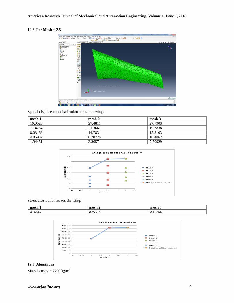
Spatial displacement distribution across the wing:
mesh 1 mesh 2 mesh 3
0.123608 0.125355 0.127295
0.0824682 0.0976335 0.0883697
0.0544441 0.056929 0.0476585
0.0284523 0.0243088 0.0259118
0.0101089 0.00536876 0.00923708
Stress distribution across the wing:
mesh 1 mesh 2 mesh 3
6520460 6632600 6645860
12.21 Analysis:
After analyzing different material properties using finite element analysis it was seen that the values obtained for
spatial displacements and stress magnitudes acting across the wings are different for varying young’s modulus and
poisson’s ratio. This depends on number of factors accompanying the behavior of the wing and the respective forces
acting on it depending on the size, mass, and characteristics and properties of the material used. On analysis it was
found that out of the three materials tested on Abaqus, aluminum was found to be having acceptable spatial
displacements over fiber glass and thermoplastic polyester elastomer. Also, considering the stress components and
magnitudes, it was found that fiber glass and thermoplastic polyester elastomer had a wider section of stress factors acting on it due to the lift force at the center of pressure, however in case of aluminum, the stress magnitudes were
lower and at a concentrated section of the center of pressure balancing the geometry of the aircraft and giving it a
much stable structure for flight purposes.
XIII. OPTIMIZATION
13.1 Airfoil Parameterization
The first step in optimizing an airfoil is choosing the design variables and generating the relationships between those
variables and the upper and lower surface contours. The surface contours are used in finite element or finite
difference calculations to determine the airfoil flight behavior. The design variables used are those defined by

American Research Journal of Mechanical and Automation Engineering, Volume 1, Issue 1, 2015
www.arjonline.org 15
Jacobs, Ward, and Pinkerton [1] in their pivotal NACA Report No. 460 from 1933. These are max camber (m), and
max camber location (p), and max thickness (t). Another design variable was added, trailing edge angle (a), in order
to give greater control over the airfoil shape and allow for positive pitching moments. The design variables are
illustrated in Figure below.
Figure1. Illustration of airfoil design variables
Report No. 460 also gives equations for translating the design variables to surface contour equations. The
derivations assume particular forms for both the surface and mean line curve fitting. The same forms are assumed in
the present analysis, with the exception of the trailing edge angle. In all equations it is assumed that the chord length
is one unit, so that all other dimensions are scaled to the chord length. The half thickness on either side of the mean
line is given by the equation
432 10150.028430.035160.012600.029690.02.0
xxxxxt
yt (1)
This quantity will need to be modified by the angle between the mean line and the x-axis, designated by
dx
dyc1tan (2)
where yc is the location of the mean line for a particular value of x. The equation for the mean line for px is
given by
2
22 xpx
p
myc (3)
Report No. 460 gives the mean line equation for px as
2
2221
1xpxp
p
myc
(4)
However, in order to account for the trailing edge angle in the present analysis, the equation needs an additional
coefficient. In the present analysis, cy is assumed as cubic for x > p. The same boundary conditions are used as in
Report No. 460 with the addition of a requirement on the derivative at x=1,
adx
dy
x
c
1
1tan (5)
The resulting equation set is solved in Matlab for cy at x > p using a linear equation solver. Finally, the upper and
lower surface coordinates are given by
cos
sin
cos
sin
tcl
tl
tcu
tu
yyy
yxx
yyy
yxx
(6)

American Research Journal of Mechanical and Automation Engineering, Volume 1, Issue 1, 2015
www.arjonline.org 16
Since a finite element type solver will be used to determine flight characteristics, the upper and lower surface
profiles need to be calculated at discrete points. 150 elements were used to cover the entire distance from 0x to
1x . In order to improve the accuracy of the profile at the leading edge, the chord length was divided into three
regions. The element count is given in Table 1.
Table 1: Airfoil surface element count.
X1 X2 # of Elements
0 0.03 50
0.03 0.1 50
0.1 1 50
13.2 Airfoil Analysis with XFoil
For airfoil optimization, a reliable solver must be employed to analyze airfoil designs. XFoil is widely known for its
accuracy and ease of use. It was chosen for optimization for these reasons and also because it can be controlled by
Matlab via simple batch files. XFoil is a freeware multi-variable analysis package that uses an airfoil shape input
directly using a locus of points in a text file. The aerodynamic analysis of the given airfoil is done for a viscous solution using a modified panel method to determine the aerodynamic coefficients of lift, drag, moments at user-
specified angles of attack (for a given Reynolds number). The total velocity at each point on the airfoil surface and
wake, with contributions from the free stream (flow around the airfoil), the airfoil surface vorticity (tendency for a
fluid to spin), and the equivalent viscous source distribution, is obtained from the panel solution with the Karman-
Tsien correction added (a nonlinear correction factor to find the pressure coefficient of a compressible, inviscid
flow). This is incorporated into the viscous equations, yielding a nonlinear elliptic system which is readily solved
by a full-Newton method [2]. XFoil consists of a collection of menu-driven routines controlled via a dos-based
command prompt. Outputs for lift, drag, and moments may be written to a text file for storage or external
manipulation.
13.3 Mathematical Modeling
To construct the optimization, first a suitable objective function must be chosen. A common optimization is the
aerodynamic efficiency, lift/drag. A useful efficient airfoil will have good lift/drag performance over a broad range of operating conditions, most importantly over a broad range of angles of attack (α). Optimization at a single α
often results in poor performance of off-design conditions. In an attempt to achieve good performance over a range
of α, three different angles of attack were averaged in the objective function. The objective function chosen was:
Min3
///)(
)7()4()5.1(
DLDLDL CCCCCC
xF (7)
After choosing the objective function, a suitable set of constraints is required. Side constraints are imposed on the
design variables, determined by engineering judgment. A major concern with using XFoil for optimization is that, if
the airfoil shape is not “smooth” enough, XFoil itself has difficulty converging on a solution to the Newtonian
system representing the flow field. This concern factors heavily into choosing the side constraints. These side constraints represent the first eight constraints in the optimization. The final ranges of design variables are
presented in Table 2 below. The first three parameters are fractions of the total unit-length chord.
Table 2: Side constraints
Parameters m p t a (°)
Minimum 0 0.15 0.075 -10
Maximum 0.04 0.6 0.2 15
In addition to the side constraints, it is often desirable to constrain some of the aerodynamic parameters themselves.
In the present optimization, multiple cases are considered; one in which only side constraints are present and another
in which the aerodynamic pitching moment (Cm) is constrained. For the case in which Cm is constrained it
represents the ninth constraint as follows:

American Research Journal of Mechanical and Automation Engineering, Volume 1, Issue 1, 2015
www.arjonline.org 17
0)9( min, mm CCg (8)
In addition to the design variables describing the airfoil shape, several parameters are set within XFoil. These
parameters are angle of attack for the analysis, Reynolds number, and Mach number. In the present analysis, angle
of attack is considered in the objective function, as already discussed. Reynolds number is varied from 80,000 to
300,000, and Mach number is held at zero.
13.4 Optimization Scheme
In the optimization, XFoil is used as a “black-box” function that receives an input airfoil shape and gives
aerodynamic coefficients as an output. There is no known functional form of the output based on the input design
variables; XFoil uses a complex set of equations to approximate the flow field around the airfoil. The flow field functions themselves are highly nonlinear. In addition to a nonlinear design space, aerodynamic constraints such as
the pitching moment are also unknown and nonlinear.
To deal with nonlinearity in the function itself and the constraints, a Sequentially Unconstrained Minimization
Technique (SUMT) is employed. SUMT methods add constraints to the objective function in the form of penalty
functions. That is, any violated constraint penalizes the objective function so that the minimization technique steers
towards feasible space. SUMT methods rely on numerous individual unconstrained minimizations of the pseudo-
objective function which includes the penalty terms. Each time a minimum of the pseudo-objective function is
performed (the stationary point is found) the penalty terms are updated so that the next iteration will bring the
stationary point closer to the true constrained optimum.
There are a number of SUMT methods which would work for the airfoil optimization problem. Of these, the
Augmented Lagrange Multiplier (ALM) method is chosen because it includes the Kuhn-Tucker conditions for
optimality and because it does not require the penalty coefficient to approach a singularity in order to reach the true optimum. The ALM method includes the Lagrange multipliers in the penalty terms and updates them with each
iteration. When the optimum is reached, the Lagrange multipliers will have also converged to their optimum values.
ALM also includes a separate penalty term rp which may be increased with each iteration but does not have to be. In
the present analysis, rp is increased each time because it helped keep the initial steps from going too far into
infeasible space, limiting XFoil convergence issues.
To find stationary points, the Broyden–Fletcher–Goldfarb–Shanno (BFGS) algorithm is implemented. BFGS is a
first-order variable metric method which stores information about previous search directions in order to improve
future ones. It stores this information in a matrix which approximates the inverse Hessian at the stationary point and
is updated with each step. However, since the objective function is not quadratic, it is sometimes necessary to
restart the method with a steepest descent direction to prevent ill-conditioning of the inverse Hessian approximation.
BFGS was found to be quite efficient for the optimization—much better than a simple steepest descent method—and seemed to be less prone to getting stuck in local minima as well. The BFGS implementation was also compared
against Matlab’s fminsearch function and consistently achieved a better minimum in the same amount of time or
less.
Within the BFGS stationary-points search, it is necessary to perform a 1D search to find the optimum step size each
time a search direction is calculated. To perform this 1D search, the minimum is first bounded, then 8 iterations of a
Golden Section search are performed to refine the bounds, and finally a cubic interpolation is applied to the last four
points of the refinement step.
The overall minimization algorithm is made up of three levels: the top-level ALM method, within which is a BFGS
search for stationary points, which in turn contains a 1D search for the optimal step size in the search direction. The
entire algorithm is programmed in Matlab, which also creates the airfoil from the four parameters, runs XFoil via a
batch file, and reads outputs generated by XFoil. The algorithm is outlined in the flowchart below.

American Research Journal of Mechanical and Automation Engineering, Volume 1, Issue 1, 2015
www.arjonline.org 18
Figure 2. Optimization Scheme
13.5 Optimization Results
XFoil is a low Reynolds number solver. It works most reliably for Reynolds numbers on the model-aircraft scale,
about 50,000 – 500,000. Our optimization was run for both pitching moment constrained and unconstrained cases at
Reynolds numbers of 80,000, 200,000, and 300,000. Cm was required to be greater than or equal to zero for the constrained case. The results are presented in tabular form below.
Table 3: Optimization Results
Re
Cm
constraint
Average
Lift/Drag
Min
Cm
Max
Camber
Max
Camber
Location
Max
Thickness
TE
Angle
ALM
Iterations
80000 none 45.54 -0.1065 0.0399 0.3193 0.0777 8.947 23
200000 none 77.11 -0.1231 0.0396 0.3913 0.0955 10.627 39
300000 none 90.89 -0.1341 0.0395 0.3903 0.1007 12.136 31
80000 ≥ 0 28.13 0.0004 0.0174 0.1799 0.0750 -3.464 24
200000 ≥ 0 48.0926 0.0003 0.0340 0.2730 0.0757 -5.005 31
300000 ≥ 0 58.50125 0.0001 0.0395 0.2826 0.0761 -5.545 26
The figures below show the optimal airfoils with no pitching moment constraint.
Figure 3. Airfoils drawn to scale

American Research Journal of Mechanical and Automation Engineering, Volume 1, Issue 1, 2015
www.arjonline.org 19
Figure4. Airfoils compared
The optimal airfoils with no Cm constraint all exhibit high camber, either at or near the upper side constraint. The
max camber location does not change much with increasing Reynolds number. Thickness and trailing edge angle
increase with increasing Reynolds number.
Figure5. Lift/Drag Results
As expected, lift/drag increases with Reynolds number. The optimal airfoils with no Cm constraint perform well across a broad range of angle of attack, which was the original goal of the optimization (1.5°, 4°, and 7° were
included in the objective function). For 80,000 and 300,000, one of the three points averaged in the objective
function has a “spike,” which is also not uncommon in optimization.
The figures below show the optimal airfoils with Cm constrained to be greater than or equal to 0.
Figure6. Airfoils drawn to scale

American Research Journal of Mechanical and Automation Engineering, Volume 1, Issue 1, 2015
www.arjonline.org 20
Figure7. Airfoils compared
The most striking aspect of the Cm-constrained airfoils is the negative trailing edge angle, which keeps the pitching
moment positive. The airfoil at Re of 80,000 also exhibits much lower camber than the others (camber is directly
related to Cm). All airfoils are at or near the lower bound on thickness, but camber increases with increasing
Reynolds number. To offset this, trailing edge angle decreases with increasing Reynolds number.
Figure8. Lift/Drag Results
As in the previous case, lift/drag increases with increasing Reynolds number. However, the pitching moment constraint decreases the lift/drag performance for the optimal airfoils. Additionally, the Cm-constrained airfoils do
not perform as well over the whole range of angle-of-attack, but tend to reach a peak at around 7°.
13.6 Practical Optimization: Airfoil Design Considerations
13.6.1 Application
The actual application of the airfoil is the most important consideration that not only affects the design constraints,
but also determines which aerodynamic properties need to be optimized. In some situations the ratio of lift over
drag is not the most important design aspect and some airfoils are designed to produce as little drag as possible with
a constraint on lift. Some airfoil designs may not generate any moment on an aircraft (such as tailless aircraft) while
others may utilize lifting tails to compensate for large moments created by high camber airfoils that maximize lift.
The air speed and altitude at which an airfoil is to operate (and thus the Reynolds number and air density it will
experience) are critical to the optimization of any given airfoil; the optimization scheme for an airfoil to be used on a
wind turbine will vary drastically from that of a glider or supersonic aircraft. The change from an incompressible flow regime (subsonic) to a compressible one (transonic, supersonic and hypersonic) will affect the overall design of
an airfoil dramatically. Airfoil design optimization for compressible flow must take into account not only the drastic

American Research Journal of Mechanical and Automation Engineering, Volume 1, Issue 1, 2015
www.arjonline.org 21
change in air density the airfoil will experience as it changes from subsonic to supersonic, but also the development
of shock waves at leading and trailing edges of the airfoil.
13.6.2 Aircraft Optimization
Aircraft optimization is a balancing act between aerodynamic efficiency (usually represented by coefficient of lift
over drag) and the multi-disciplinary design optimization of the aircraft itself. In many cases a varying airfoil shape
may be utilized over the entire wing-form; such as in “flying wing” aircraft that tend to experience pitch or roll stability issues. Constraints may be added to the design of a given airfoil because of limitations due to aircraft
structure and controls. An airfoil may be optimized for a given lift over drag regime, but may not be large enough to
support the internal structure necessary for the amount of lifting force, deflection, and stress on the wing itself. An
airfoil may also be optimized aerodynamically but the control surfaces needed to pilot the aircraft may be
impractical due to large moments created by high camber values. Invariably a compromise and balance must be
reached between the aerodynamic, structural and control aspects of an aircraft’s design optimization.
XIV. GEOLOGICAL SURVEY AND GEOPHYSICAL WORK[4]
Geological surveys, for which a UAV is ideally, suited to criss-cross a region under computer control for up to
30 hours at a time, using GPS signals and precision flight control, to follow an exact flight path. The value of a
UAV is its ability to operate in a “low, slow, fly mode”, down to 20m above ground level, to get better
resolution.
The typical cost of a manned aircraft survey is in the range from $15 to $20 per line mile, whereas it drops to $2
to $3 per line mile for a lower cost, pilotless, UAV.
The small physical size of the UAV and its low metal content relative to that of a manned aircraft, enables the UAV
to make less of a perturbation to the magnetic and gravitational fields being measured, enabling more accurate
measurements of:
Field strength and field gradient measurements:
of magnetic field strength (“aeromagnetic”)
of the vertical and horizontal magnetic field gradients
of the differential gravity field (gradiometry)
Electromagnetic measurements:
of electromagnetic phase and magnitude reflection ratios over a wide frequency
time domain electromagnetic pulse reflection signal measurements
Ground Penetrating RADAR sensing of ground and rock dielectric constant
Other measurements:
gamma ray spectrometer and neutron reflection level measurements
using a photo-ionization detector, to measure ethane levels in the air
high resolution multi-spectral imaging, including thermal imaging
XV. SENSORS ANALYSIS
15.1 AHRS and INS Sensor
The POLAR is a high-end, MEMS-based Attitude and Heading Reference System (AHRS) and Inertial Navigation
System (INS). It is perfect for system integration in avionics packages or other attitude sensing applications, and
includes:
Attitude Heading & Reference System (AHRS)
Inertial Measurement Unit (IMU)
Inertial Navigation System (INS)
American Research Journal of Mechanical and Automation Engineering, Volume 1, Issue 1, 2015
www.arjonline.org 22
Air Data System (ADS)
GPS
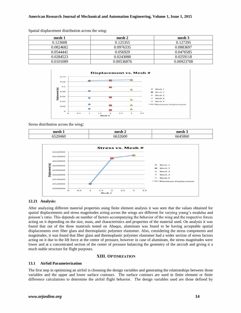
Redundancy built into the POLAR software allows it to survive individual sensor failures while maintaining
accurate estimates of attitude and position. For maximum safety the POLAR features two sets of sensors: the first is
a set of very high quality MEMS accelerometers and gyros, used for normal operation (the Tech Spec tab relates to
these sensors). In addition, the POLAR has another set of gyros and accelerometers in a single, tiny chip (approx 3 x 4 x 1mm) which acts as backup. This second set is not used in normal operation, but the POLAR activates them in
the unlikely event of a failure.
It is also suitable for:
RPAS/UAVs (fixed wing, helicopter, multi-rotor) where a defined Flight Control solution exists
High speed target drones
Payload control (incl. gyro-stabilizing and geo-referencing cameras/antenna)
Satellite and TV antenna pointing
Automotive, maritime and robotics applications
Manned aviation (data source for EFIS)
Motorsport vehicle dynamics telemetry
Technical Specifications
Electrical:
Voltage Supply: 9V to 36V DC
Power Consumption: 1W
GPS:
Antenna: Active or Passive
Antenna Connector: HFL and HLF to SMA adaptor
Antenna Power Supply: 3V
Sensitivity: -144 dBm
ADS (Air Data System):
Air Speed (Extra Low): 5 to 80 Kt
Air Speed (Low): 25 to 150 Kt
Air Speed (Normal): 35 to 250 Kt

American Research Journal of Mechanical and Automation Engineering, Volume 1, Issue 1, 2015
www.arjonline.org 23
Air Speed (High): 45 to 450 Kt
Altimeter: -2.000 to 30.000 ft
Altimeter Accuracy: 50ft
Altimeter Resolution: 0.5ft
IMU (Inertial Measurement Unit):
Sampling Rate: 1 kHz
Accelerometers:
Accelerometers Range: +/-16 g (all axis)
3dB Bandwidth: 400 Hz
Noise: 0.52 mg/sqrt(Hz)
Rate Gyro Range:
Gyro Range: 2000o/s
3dB Bandwidth: 77Hz
Noise: 0.015o/s/sqrt(Hz)
Mechanical/Environment:
Size (mm, H x W x L): 22 x 40 x 82
Weight: 76 g
Humidity: Up to 90% RH, non-condensing
Temperature Range: -40oC to +85oC
Shock Survival: 500g 8ms ½ sine
Mating Connector: MICRO-D Type Male 15p
15.2 HERKÜL – 1D, 24 VDC – 2 x 50 A, Dual Axis Servo Controller
Servo controller developed for small to medium caliber gun and missile platforms, electro-optics and radar
systems
100 A total current output in independently driven two lines
Torque, speed and position control, integral stabilization control
Adaptability to mission requirements owing to DSP technology
Conformance to military specs (MIL-STD-810 & MIL-STD-461)
Broad range of interface and sensor options
Test interface and automated built-in test feature
Product Features
High efficiency motor control using ASELSAN servo controller technology
Torque, speed, position and stabilization control
Application specific configuration (parametric motion limits, no-fire zone, maximum speed and acceleration)
Extensive built-in self-test
Over-heat and over-current protection

American Research Journal of Mechanical and Automation Engineering, Volume 1, Issue 1, 2015
www.arjonline.org 24
Fanless cooling and silent operation
Technical Data
Drives two 50 A brushless DC motors
18-32 VDC supply voltage
Peripheral interfaces:
Analog
Serial (CAN, RS-232/422)
Resolver
Encoder (SSI/EnDat)
Dimensions: 310 mm x 230 mm x 100 mm
Weight: 7 kgf
Conforms to MIL-STD-810 & MIL-STD-461
Operating temperature: -40°C − +62 °C
Storage temperature: -40 °C − +75 °C
Vibration: 15 − 2000 Hz, 0.1 g²/Hz
Shock: 40 g, 11 ms MIL-STD-810
EMC/EMI: MIL-STD-461
15.3 TMX6
It is a rugged camera module with a remote sensor head designed for integration in Airborne payloads. The camera
incorporates an automatic shutter and gain control and a video contrast enhancement module to ensure maximum
detection and recognition ranges when operated in long focal range applications.
The TMX6 camera has 1/3’’ or ½’’ CCD imager with either peaked Green or peaked Near infrared response. The remote head design in combination with the stable Line of Sight makes system interfacing relatively straightforward.
Key Features
Monochrome CCIR or RS170
Peaked Green or NIR response
Stable line of sight
Automatic exposure control
Contrast enhancement
Remote head
15.4 MWIR-60
The MWIR-60 uses a proprietary HyperPixel Array (HPATM) SNAPSHOT technology to capture spectral and spatial information in one instantaneous video frame, thereby eliminating motion artifacts and maximizing signal-to-
noise. It operates over the mid-wave infrared band and is designed to interface with virtually any foreoptic, from
telescope to microscope.
Key Features:

American Research Journal of Mechanical and Automation Engineering, Volume 1, Issue 1, 2015
www.arjonline.org 25
Can Identify Spatial and Spectral Features in a Single Video Frame
Ideal for Moving Platforms and Transient Events
No Moving Parts
Unique Patent Pending Technology
Data Cube: 17 x 13 x 60
17 x 13 spatial
60 spectral
Spectral Band: 3-5 µm
Spectral Resolution (average): 34 nm/bin
Data Rate: Up to 60 cubes/sec
Power: 14 Watts
Field of View: 6.7° x 5.4° (WFOV), 4.8° x 3.6° (NFOV)
Dimensions: 3.5” W x 5” H x 19.2” L (WFOV), 3.5” W x 5” H x 17.8” L (NFOV)
Weight: 13.1 lbs
Power: 14 Watts
Optional add ons:
Analysis Software
Compatible Computer
Lenses
Environmental Housings
15.5 Model 20 / 24 Infrasound Sensor
Chaparral Physics sensors combine rugged construction with wide bandwidth and low noise to ensure accurate
measurements in the most demanding of environments. They have no need for altitude adjustments, and are
carefully designed to reduce the effect of environmental temperature variations and mechanical vibrations. From the
Ross ice-shelf in Antarctica through the rain forests of Central America to Alaska’s tundra, Chaparral Physics
microphones have proven their reliability and value as the finest infrasound measuring instruments in the world.
Some of the important features, which give this sensor an advantage in real world installations include:
Robust physical build quality with stainless steel and sealed electronics
Built in manifold for connecting to a noise reduction array (M24 only)
High dynamic range
Low noise floor
Low power consumption
Differential output
11 octave bandwidth that includes the low audio spectrum (0.10 Hz to 200 Hz)
Low Cost
The Model 20 and 24 are an excellent choice for any application requiring a high resolution infrasound sensor in a
small form factor at a low cost. It excels at accurately recording signals which span the low audio/infrasound
boundary

American Research Journal of Mechanical and Automation Engineering, Volume 1, Issue 1, 2015
www.arjonline.org 26
Specifications:
Nominal Sensitivity: 0.4 volts/Pa @ 1 Hz, 90 Pa full scale range
Output:
Output type: Differential
Maximum: 36 volts peak-to-peak (signal+ to signal-)
±9 volt max, signal to ground
Frequency Response: Flat to within +0, -3 dB from 0.1 Hz to 200 Hz
Flat to within +0, -0.5 dB from 0.3 Hz to 50 Hz
Self noise: Less then 0.63µPa2/Hz @ 1 Hz (-62dB Pa2/Hz, rel to 1 Pa)
Dynamic range: 101dB low gain (@ 0.8mPa RMS self noise)
Output Impedance: 150Ω non-reactive (recommended load > 10 kΩ)
Short circuit protected: signal+ to signal– and signal to ground
Power Requirements:
DC Source: 12 volts, (9-18 volts) DC, reverse voltage protected.
Current Drain: Less than 40 ma @ 12 v
Physical:
Operating Temperature: -40º C to +65º C
Humidity: 95% (non-condensing)
Dimensions M24: 5.5” (14 cm) maximum height, 9” (23 cm) maximum diameter
Weight M24: 5.3 lbs (2.4 kg), for 4-port version
Std Acoustic inlets M24: 4 ports (maximum 12), male, Garden-Hose- Thread.
Dimensions M20: 7” (18 cm) maximum height w/ legs, 5.75” (14.6 cm) w/o
legs, 7” (18 cm) maximum diameter
Weight M20: 3.25 lbs (1.5 kg) w/legs, 2.75 lbs (1.25 kg) w/o legs
15.6 SQ01 Hydrophone
The SQ01 is a highly sensitive, low-cost hydrophone that can also be used as a low-power projector. The
polyurethane-encapsulated hydrophone will withstand continuous immersion in isoparaffinic hydrocarbon fluids and
sea water.
Specifications:
Voltage sensitivity: -193.5 +/-1.5 dBV
Charge sensitivity: 440 nC/bar
Capacitance: 31 nF +/-15%
Capacitance variation with temperature: 0.33% increase per oC
Capacitance variation with pressure: 8% loss at 1000 m
Operating depth: down to 1000 m
Frequency response: flat from 1Hz to 5000Hz
Max. Drive Voltage: 50V
Diameter: 30.7mm

American Research Journal of Mechanical and Automation Engineering, Volume 1, Issue 1, 2015
www.arjonline.org 27
Length: 95.2mm
Mass: 75g
Electrical Insulation between leads: >500 M ohms
15.7 Echosounder Transducers (SX18)
Characteristics:
Resonance Frequency: 500 kHz
Beam Pattern: 2.5 degrees
Transmit Voltage response: 165 db
Receive Voltage response: -185 db
Mechanical Q: 10 db
Rated Power: 600 RMS Watts
Bandwidth: 50 kHz
Termination: P=pigtail
Depth: 100m
Transformer: OPT
XVI. UAV CONCEPT
The Unmanned Air Vehicle has a complex electronic, communication, sensor and computation systems content,
all of which need to operate reliably, for up to 30 hours.
Ideally two or more engines, with their associated electrical power generators, provide some degree of back-up,
in the event of an engine failure.
The successful Unmanned Air Vehicle needs to combine state-of-the-art miniaturized, low power, navigation
sensors, communications electronics and digital flight automation electronics, with an efficient, reliable, low
vibration engine, on a high performance air frame.
XVII. QUANTUM COMMUNICATION SYSTEMS[5]
In this section, a linear time-invariant multivariable UAV plant is considered.
The reference model can be expressed as:
where, xp(t), xm(t) are state vectors; yp(t), ym(t) are output vectors; u(t) are control input vectors. Ap, Am, Bp, Bm, Cp,
Cm are system state matrices, input matrices, and output matrices, respectively.
In quantum computation, 0 and 1 denote the two basic states of micro‐ particles, which are termed quantum bits
(qubits). An arbitrary single‐ qubit state can be expressed as the linear combination of two basic states. The state of a qubit is not only 0 and 1 , but is also a linear combination of the state, which is usually termed a superposition
state, namely,

American Research Journal of Mechanical and Automation Engineering, Volume 1, Issue 1, 2015
www.arjonline.org 28
probability of 2 2.
Due to the collapse of quantum states caused by observation, the quantum bits can be seen as a continuous state
between 0 and 1, until it has been observed. The existence of a continuous state qubit and behavior has been
confirmed by a large number of experiments, and there are many different physical systems that can be used to
The actuator is one of the most important components in an aircraft system. Various types of actuator faults have
been performed, including actuator effectiveness, decrease due to control surface impairments, floating faults,
saturation faults, etc. To formulate the fault‐ tolerant tracking control problem, the loss‐ of‐ effectiveness fault is established for this research. Faults that are developed in a linear system can be represented by an equation:
The error of the state variables between the plant and model is defined as:
The control objective: for the controlled plant with faults and parameter uncertainties, an adaptive control law is
designed to track the reference model for any u.
Adaptive control based on Popov hyperstability theory and quantum information technology
UAV flight control systems can be divided into longitudinal channel control and lateral channel control. The control
surfaces are elevator, aileron and rudder, respectively. In a normal case, due to the strong coupling between the
longitudinal and lateral channels, the control law design becomes very complex, so the longitudinal and lateral
channel control must achieve decoupling. Then the longitudinal and lateral control can be designed for UAV flight
control systems, respectively. In this study, the integrated control law is designed for a UAV flight control system’s
longitudinal and lateral channel using the quantum bits state of the quantum‐ control technique. The quantum control module shows the three quantum bits’ state description and control, and the specific description of three
quantum bits’ probability amplitude for the UAV quantum control module can be seen in the table below.

American Research Journal of Mechanical and Automation Engineering, Volume 1, Issue 1, 2015
www.arjonline.org 29
Probability amplitude on quantum control module
XVIII. CONCLUSION
Airfoil optimization using modified parameters, with XFoil as the analysis engine and an Augmented Lagrange
Multipliers optimization scheme, has been successfully demonstrated with very good results. The optimization
could be extended to use a different objective function and different aerodynamic constraints, if desired. For greater
usefulness, the parameterization could be extended to include additional design variables. Equation (1), which
describes the thickness distribution of the top and bottom surfaces about the mean camber line, contains 5
coefficients, which are held constant in both the airfoil four-digit series and the modified parameterization, which is
used in this study. Some or all of those coefficients could be related to the airfoil shape and treated as additional
design variables for greater control over the airfoil shape and presumably better optimization results. It is
recommended that the leading edge radius and maximum thickness location be included as design variables in future work.
Therefore, considering the advantages offered by an efficient design and development of an Ultra Long Endurance
UAV can provide solutions for exploring and exploiting underneath waterbeds for petroleum in specific to
geographical regions where reaching out can be considered as one of the hardships to carry out the seismic data
collecting and research. On studying several characteristics and properties of the Ultra Long Endurance UAV, it was
found to be quite suitable for the very specific purpose of mineral exploration.
Moreover, the instruments, devices, and sensors been taken into account for the study, determines quite realistic
approach for data collection, which plays an important role for research based purposes. The list of recommended
data in this study are sufficient enough to gather information to carry out mining research specifically directed to
petroleum as a mineral in quite high efficiently.
The UAV endurance to run for quite high range of time limit provides better efficiency and timesaving for seismic data collecting. The aircraft can fly efficiently under varying range of temperature and pressure environments that
are usually found above water bodies that are considered by the specialists for seismic mining prone regions. Also,
the efficient functioning of the Ultra Long Endurance UAV at high altitudes provides the possibility of its
functioning in varying climatic conditions.
The seismic ships that are currently used for mineral exploration purposes are quite expensive and on top needs
people to work and operate the ship and instruments that it has on board. It requires a really high budget to train
those people and to provide them wages upon hiring. This sums up to a really high budget focusing towards seismic
data collecting, excluding processing. However, using UAVs cuts down the budget to a comparatively smaller
amount. No humans are necessary to be hired for data collecting purposes since it is an unmanned aircraft. Also, a
UAV can work non-stop for any extreme atmospheric conditions. The seismic ships usually are in the water for
about 6 months in a year, however, a UAV can work for across the whole year, accelerating and providing a
relatively large data for mineral researchers. And lastly, the cost of building an Ultra Long Endurance UAV is quite less than that of a seismic ship. The equipment and instruments used in the ships were of a relative large sizes,
however those used in the UAV, as recommended in this report, serves to be much more efficient, advanced,
precise, and of a much relative smaller size to accommodate on the UAV.

American Research Journal of Mechanical and Automation Engineering, Volume 1, Issue 1, 2015
www.arjonline.org 30
There exists several disadvantages and inaccuracies in using UAVs over seismic ships, however considering the data
collected with respect to time between the two and the average cost and the budget analysis for the process to
undertake, UAVs seems much efficient on those factors.
Besides that, security of data and its processing can be one of the major criterion to be considered by the agencies
and firms that deals with the seismic data collection. There have been several incidents happened that have dealt
with the drowning of the seismic ships or loosing collected data while transference from the ships to the processing center. In order to prevent such incidents, quantum information technology is taken into usage, while remain a
theoretical concept so far until the technology is physically out for industrial practice. The quantum technology
disregard the case of data hacking, since its designed quite intricately where the base of the system works on
quantum interference, which is totally unsupportive of computer technology which we use at the current time period.
Quantum technology lays the foundation of cubits, which has so far been guaranteed as the fastest mode of data
transmission and procession than normally used advanced databases.
XIX. ACKNOWLEDGEMENTS
I would like to thank Dr. Sridhar Condoor, Aerospace & Mechanical Engineering Department Chair – Saint Louis
University, for supervising the research and providing innovative ideas to approach the problem statement. I thank Dr. John George and Dr. William Thacker for providing insights and expertise on fluid mechanics, and quantum
computation and information technology, respectively, that greatly assisted the research.I would also like to show
the gratitude to Mr. Krishan Gupta, Chief After-Sales and Service Officer – Prakash Agricultural Industries, and Mr.
JuergenBleisinger, Rt. General Manager – Schlumberger Ltd., to provide essential industry standards and procedures
that are currently undertaken for seismic acquisition.
REFERENCES
[1] Jacobs, Eastman; Kenneth Ward, and Robert Pinkerton. The Characteristics of 78 Related Airfoil Sections from Tests in the
Variable-density Wind Tunnel, Report No. 460. National Advisory Committee for Aeronautics: November 1933.
[2] Drela, Mark, and Youngren, Harold. XFOIL Subsonic Airfoil Development System. XFOIL 6.9 Primer. <http://web.mit.edu/drela/Public/web/xfoil/xfoil_doc.txt>. Updated November 2001. Accessed May 18, 2010.
[3] Atteberry, Janathan (2013). Discovery Communications, LLC. Extracted from: http://www.discovery.com/tv-shows/curiosity/topics/10-real-world-applications-of-quantum-mechanics.htm
[4] Emaco Group. Unmanned Aircraft Systems Part I. http://www.emacogroup.eu/UAV%20geological%20survey.pdf
[5] Chen F., Hou R., Tao G. (2012) Adaptive controller design for faulty UAVs via Quantum Information Technology. International Journal of Advanced Robotics Systems. INTECH. http://cdn.intechopen.com/pdfs-wm/41569.pdf
[6] http://www.uavnavigation.org/products/polar-imu-ahrs-ins-sensor-system
[7] http://www.aselsan.com.tr/en-us/capabilities/unmanned-systems/servo-systems/herkul-1d HERKUL 1D
[8] http://www.adimec.com/en/Service_Menu/Industrial_camera_products/Rugged_tailored_and_COTS_cameras_for_defense_and_security_applications/TMX6-series
[9] http://www.bodkindesign.com/products/hyperspectral-imaging/mwir-60/ MWIR 60
[10] http://www.gemsys.ca/products/uavs-pathway-to-the-future/ Magnetometer
[11] http://www.gi.alaska.edu/files/Flier%20Model%2020_24.pdf Infrasound sensor
[12] http://www.sensortech.ca/userfiles/file/SQ01(2).pdf Hydrophone sensor
[13] http://www.sensortech.ca/site/index.cfm?DSP=Page&ID=101 Echosounder transducer
[14] http://www.seistronix.com/ras_g.htm RAS-24 to connect the ports to the data processing unit
[15] Gundlach J. (1975) Designing unmanned aircraft systems: a comprehensive approach. AIAA Education Series. American Institute of Aeronautics and Astronautics, Inc. Virginia 21191-4344.