Applying Target Decomposition Algorithms on the Detection of Man Made Targets Using Polarimetric SAR

University of British Columbia

September, 2007

Flavio Wasniewski*, Ian Cumming

Objectives

1. Review the Detection of Crashed Airplanes (DCA) methodology applied by Lukowski et. al.

2. Test this methodology with a more diverse set of target clutters and types;

3. Compare its performance with available target detection algorithms;

4. Develop improvements to the methodology in order to give good detection performance to a range of target and clutter types.

2

Detection of Man Made Targets with Radar Polarimetry

3

High target-to-clutter ratio (not necessarily higher than in natural targets)

Dihedral scattering expected (phase information can be explored)

Polarimetric decompositions are among the most promising algorithms

Most civilian operational applications focus in ship detection

Detection of Crashed Airplanes (DCA)

Source: Lukowski et. al., CJRS, 2004

4

Promising in-land application

Tested on airplanes and low vegetation clutter

Tail and wings usually remain intact and provide dihedrals

Can it be applied to all discrete man made targets? (will dihedrals always be present?)

5

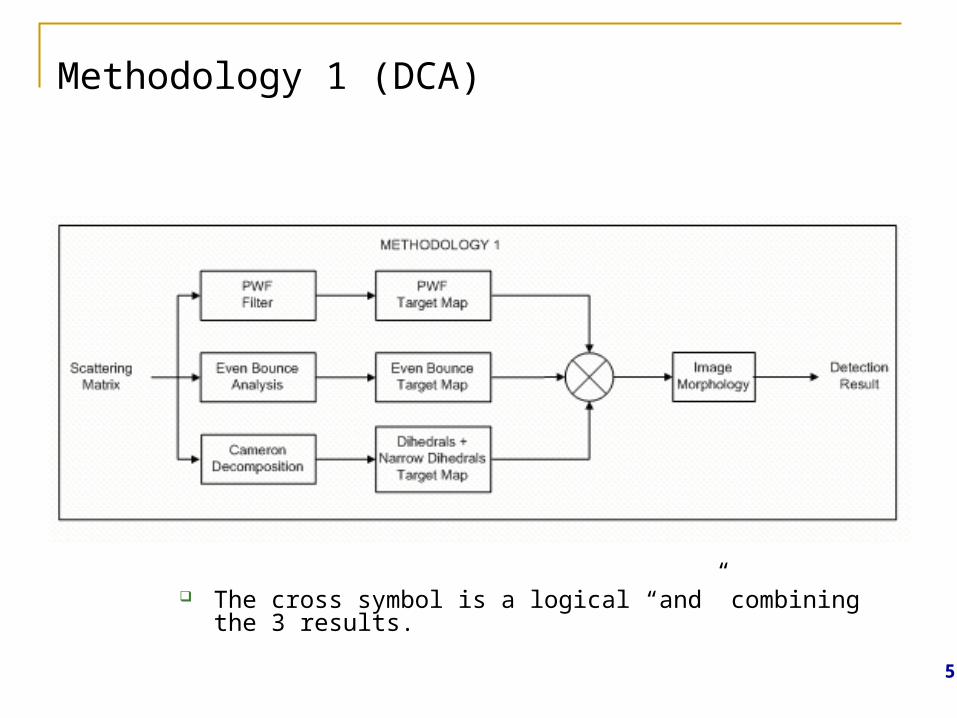
Methodology 1 (DCA)

The cross symbol is a logical “and” combining the 3 results.

6

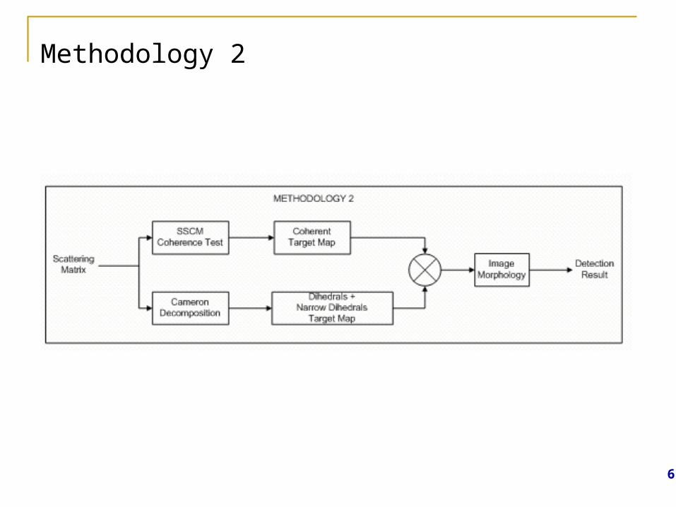
Methodology 2

7

Methodology 3

8

Methodology 4

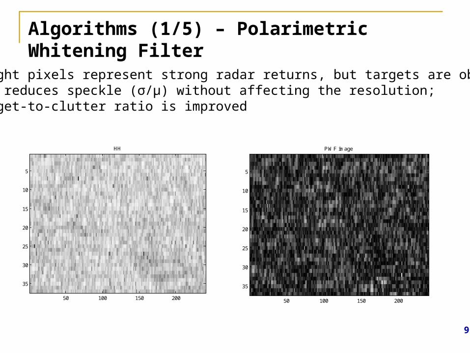
Algorithms (1/5) – Polarimetric Whitening Filter

9

Bright pixels represent strong radar returns, but targets are obscured; PWF reduces speckle (σ/µ) without affecting the resolution; Target-to-clutter ratio is improved

HH

50 100 150 200

5

10

15

20

25

30

35

PWF image

50 100 150 200

5

10

15

20

25

30

35

10

Algorithms (2/5) – Even Bounce Analysis

Explores the 180° phase shift between HH and VV

Even Bounce Image

100 200 300 400 500 600

5

10

15

20

25

30

35

40

HH

100 200 300 400 500 600

5

10

15

20

25

30

35

40

22

22 hv

vvhheven S

SSE

11

Algorithms (3/5) – Cameron Decomposition

Classifies the target according to the maximum symmetric component in one of six elemental scatterers.

10

01

10

01

00

01

5.00

01

5.00

01

i0

01

Target SM Z

Trihedral 1

Dihedral -1

Dipole 0

Cylinder 0.5

Narrow Diplane

-0.5

Quarter Wave

i

Source: Cameron, 1996

12

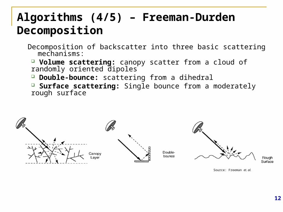
Algorithms (4/5) – Freeman-Durden Decomposition

Decomposition of backscatter into three basic scattering mechanisms: Volume scattering: canopy scatter from a cloud of randomly oriented dipoles Double-bounce: scattering from a dihedral Surface scattering: Single bounce from a moderately rough surface

Source: Freeman et. al.

13

Algorithms (5/5) – Coherence Test

Detects coherent targets based on the degree of coherence and target-to-clutter ratio.

22

2*

222.4

symp

Degree of coherence

and are the Pauli components

•Closing (dilation + erosion)•Clustering•Erasing 1 and 2-pixel detections

Morphological processing

14

Experiments: data sets used (1)

Gagetown dataset

15

Experiments: data sets used (2)

Westham Island dataset

16

17

Results – Target 21 (House Among Trees)

CV-580 data Target and clutter(Ikonos image)

18

Results – Target 21 – Methodology 1 PWF and Even Bounce

PWF Target Map (K = 2)

50 100 150 200 250 300 350 400

10

20

30

40

50

60

70

Even Bounce Target Map (K = 7 )

50 100 150 200 250 300 350 400

10

20

30

40

50

60

70

19

Cameron, PWF and Even Bounce

50 100 150 200 250 300 350 400

10

20

30

40

50

60

70

Detection Map - Methodology 1

50 100 150 200 250 300 350 400

10

20

30

40

50

60

70

Results – Target 21 – Methodology 1 Cameron combined to PWF and Even Bounce

20

Results – Target 21 – Methodology 2Coherence Test Target Map

50 100 150 200 250 300 350 400

10

20

30

40

50

60

70

Cameron and Coherence Test Map

50 100 150 200 250 300 350 400

10

20

30

40

50

60

70

Detection Map - Methodology 2

50 100 150 200 250 300 350 400

10

20

30

40

50

60

70

21

Results – Target 21 – Methodology 3

Detection map after morphology

22

Results – Target 21 – Methodology 4

Cameron + PWF + Even Bounce + Coherence Test Detection map

23

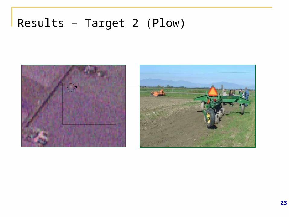
Results – Target 2 (Plow)

24

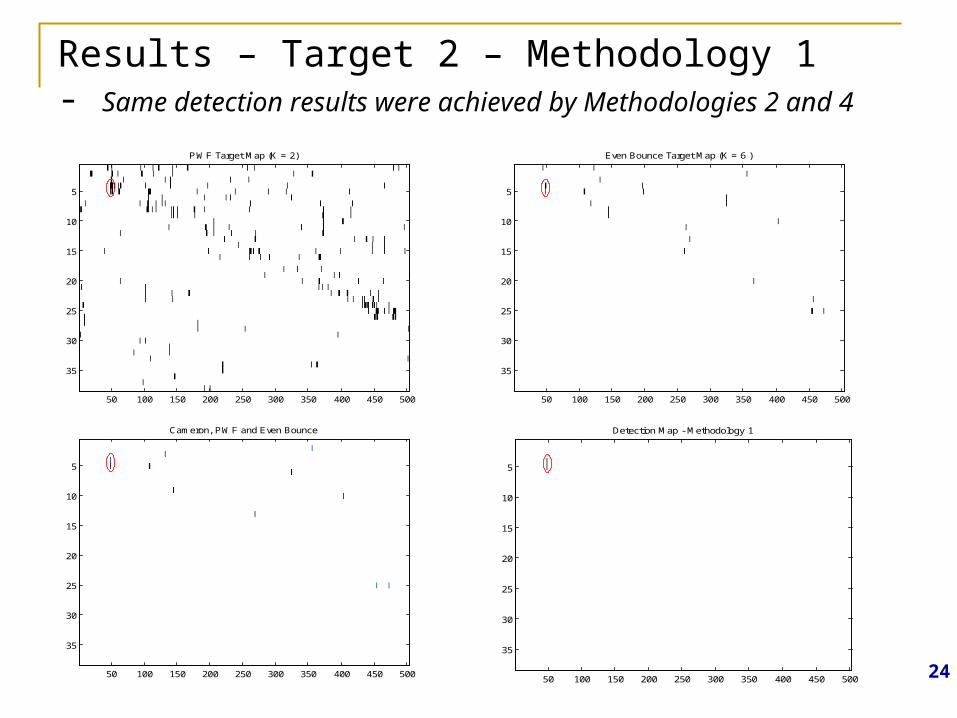
Results – Target 2 – Methodology 1 - Same detection results were achieved by Methodologies 2 and 4

PWF Target Map (K = 2)

50 100 150 200 250 300 350 400 450 500

5

10

15

20

25

30

35

Even Bounce Target Map (K = 6 )

50 100 150 200 250 300 350 400 450 500

5

10

15

20

25

30

35

Cameron, PWF and Even Bounce

50 100 150 200 250 300 350 400 450 500

5

10

15

20

25

30

35

Detection Map - Methodology 1

50 100 150 200 250 300 350 400 450 500

5

10

15

20

25

30

35

25

Results – Target 5 (Horizontal cylinders)

Cameron, PWF and Even Bounce

20 40 60 80 100 120 140 160 180

5

10

15

20

25

Cameron and Coherence Test Map

20 40 60 80 100 120 140 160 180

5

10

15

20

25

Man made target with no dihedral behaviour

No detections

26

Results – Target 7 (House)

Detection Map - Methodology 1

50 100 150 200 250 300 350

10

20

30

40

50

60

70

Detection Map - Methodology 2

50 100 150 200 250 300 350

10

20

30

40

50

60

70

Detection Map - Methodology 4

50 100 150 200 250 300 350

10

20

30

40

50

60

70

27

Results – Target 20 (Crashed Plane in Grass)

PWF image

200 400 600 800 1000 1200

10

20

30

40

50

60

70

80

90

Corner reflectors

Target

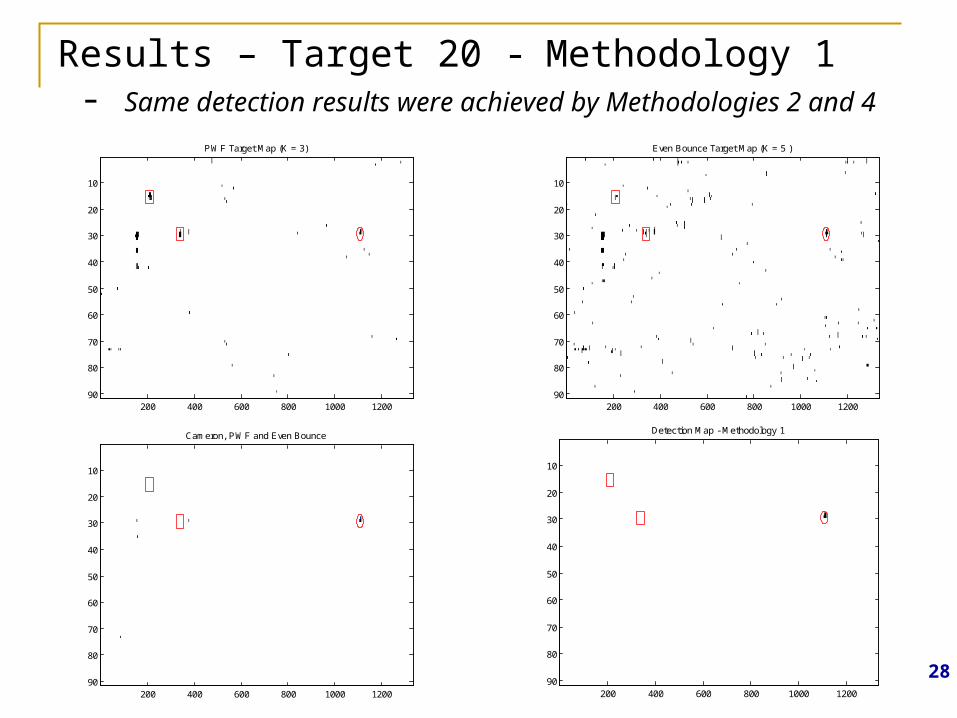
Results – Target 20 - Methodology 1 - Same detection results were achieved by Methodologies 2 and 4

PWF Target Map (K = 3)

200 400 600 800 1000 1200

10

20

30

40

50

60

70

80

90

Even Bounce Target Map (K = 5 )

200 400 600 800 1000 1200

10

20

30

40

50

60

70

80

90

Cameron, PWF and Even Bounce

200 400 600 800 1000 1200

10

20

30

40

50

60

70

80

90

Detection Map - Methodology 1

200 400 600 800 1000 1200

10

20

30

40

50

60

70

80

9028

Results

Methodology 1 Methodology 2 Methodology 4

Total False Alarm count

5 14 1

Total False Alarm Rate

210 1087 72

Methodology 1 Methodology 2 Methodology 4

False Alarm count

(Low Vegetation)0 3 0

False Alarm count

(High & medium Vegetation)

5 11 1

Total

Per Vegetation type

29

Summary

Methodology 1 (DCA) detected the targets with no false alarms when clutter is low vegetation. It did present false alarms in high vegetation;

Methodology 2 (Coherence Test) typically detects the target with few false alarms in both situations;

Methodology 3 (Freeman-Durden decomposition) generally presented high false alarm rates in this study;

Methodology 4 (DCA + Coherence Test) performs better than DCA methodology on high vegetation clutter.

30

Thank you