Applying the General Path Model to Estimation of Remaining Useful · PDF fileApplying the General Path Model to Estimation of Remaining Useful Life Jamie Coble1 and J. Wesley Hines2

International Journal of Prognostics and Health Management, ISSN 2153-2648, 2011 007

Applying the General Path Model to Estimation of

Remaining Useful Life

Jamie Coble1 and J. Wesley Hines

2

1,2The University of Tennessee, Knoxville, TN 37996, USA

[email protected]

[email protected]

ABSTRACT

The ultimate goal of most prognostic systems is accurate

prediction of the remaining useful life of individual

systems or components based on their use and

performance. This class of prognostic algorithms is

termed effects-based, or Type III, prognostics. A unit-

specific prognostic model, called the General Path Model,

involve identifying an appropriate degradation measure to

characterize the system's progression to failure. A

functional fit of this parameter is then extrapolated to a

pre-defined failure threshold to estimate the remaining

useful life of the system or component. This paper

proposes a specific formulation of the General Path Model

with dynamic Bayesian updating as one effects-based

prognostic algorithm. The method is illustrated with an

application to the prognostics challenge problem posed at

PHM '08.

1. INTRODUCTION

Prognostics is a term given to equipment life prediction

techniques and may be thought of as the "holy grail" of

condition based maintenance. Prognostics can play an

important role in increasing safety, reducing downtime,

and improving mission readiness and completion.

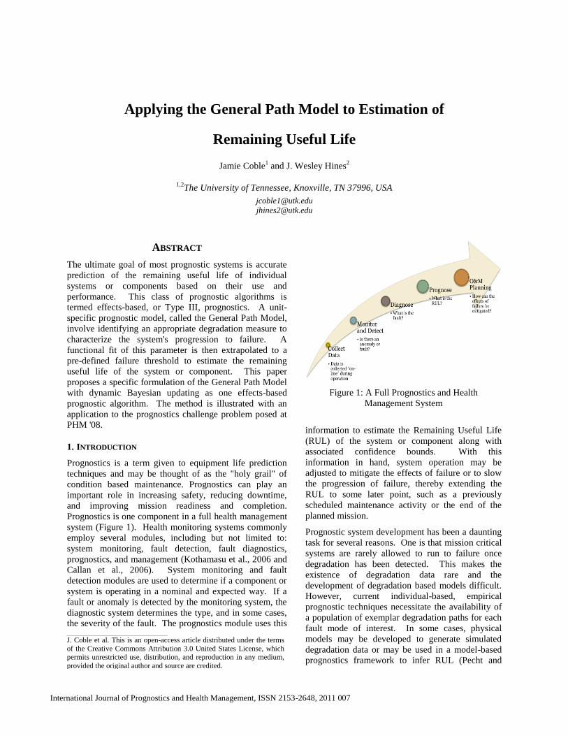
Prognostics is one component in a full health management

system (Figure 1). Health monitoring systems commonly

employ several modules, including but not limited to:

system monitoring, fault detection, fault diagnostics,

prognostics, and management (Kothamasu et al., 2006 and

Callan et al., 2006). System monitoring and fault

detection modules are used to determine if a component or

system is operating in a nominal and expected way. If a

fault or anomaly is detected by the monitoring system, the

diagnostic system determines the type, and in some cases,

the severity of the fault. The prognostics module uses this

Figure 1: A Full Prognostics and Health

Management System

information to estimate the Remaining Useful Life

(RUL) of the system or component along with

associated confidence bounds. With this

information in hand, system operation may be

adjusted to mitigate the effects of failure or to slow

the progression of failure, thereby extending the

RUL to some later point, such as a previously

scheduled maintenance activity or the end of the

planned mission.

Prognostic system development has been a daunting

task for several reasons. One is that mission critical

systems are rarely allowed to run to failure once

degradation has been detected. This makes the

existence of degradation data rare and the

development of degradation based models difficult.

However, current individual-based, empirical

prognostic techniques necessitate the availability of

a population of exemplar degradation paths for each

fault mode of interest. In some cases, physical

models may be developed to generate simulated

degradation data or may be used in a model-based

prognostics framework to infer RUL (Pecht and

J. Coble et al. This is an open-access article distributed under the terms

of the Creative Commons Attribution 3.0 United States License, which permits unrestricted use, distribution, and reproduction in any medium,

provided the original author and source are credited.

International Journal of Prognostics and Health Management

2

Dasgupta, 1995, Valentin et al., 2003, and Oja et al. 2007).

Second, if the components are subject to common fault

modes which lead to failure, these fault modes are often

designed out of the system through a proactive continuous

improvement process. Third, very few legacy systems

have the instrumentation required for accurate prognostics.

In the absence of such instrumentation, accurate physics of

failure models may be used to identify key measurements

and systems may be re-instrumented.

This research focuses on RUL estimation for soft failures.

These failures are considered to occur when the

degradation level of a system reaches some predefined

critical failure threshold, e.g. light output from fluorescent

light bulbs decreases below a minimum acceptable level or

car tire tread is thinner than some pre-specified depth.

These failures generally do not concur with complete loss

of functionality; instead, they correspond with the time

when an operator is no longer confident that equipment

will continue to work to its specifications.

Traditional reliability analysis, termed Type I prognostics,

uses only failure time data to estimate a time to failure

distribution (Hines et al., 2007). This class of algorithms

characterizes the average lifetime of an average

component operating in historically average conditions; it

does not consider any unit-specific information beyond the

current run time. As components become more reliable,

few failure times may be available, even with accelerated

life testing. Although failure time data become more

sporadic as equipment reliability rises, often other

measures are available which may contain some

information about equipment degradation, such as crack

length, tire pressure, or pipe wall thickness. Lu and

Meeker (1993) developed the General Path Model (GPM)

to model equipment reliability using these degradation

measures, or appropriate functions thereof, moving

reliability analysis from failure-time analysis to failure-

process analysis. The GPM assumes that there is some

underlying parametric model to describe component

degradation. The model may be derived from physical

models or from available historical degradation data.

Typically, this model accounts for both population (fixed)

effects and individual (random) effects.

Although GPM was originally conceived as a method for

estimating population reliability characteristics, such as the

failure time distribution, it has since been extended to

individual prognostic applications (Upadhyaya et al.,

1994). Most commonly, the fitted model is extrapolated to

some known failure threshold to estimate the RUL of a

particular component. This is an example of an Effects-

based, or Type III, prognostic algorithm (Hines et al.,

2007). This class of algorithms estimates the RUL of a

specific component or system operating in its specific

environment; it is the ultimate goal of prognostics for most

mission critical components.

The following sections will present GPM theory

including the original methodology for reliability

applications and the extension to prognostics. In

addition, a short discussion of dynamic Bayesian

updating methods to incorporate prior information is

given. Finally, an application of the proposed GPM

methodology to the 2008 PHM Challenge problem

is presented.

2. METHODOLOGY

As suggested by the “No Free Lunch” Theorem, no

one prognostic algorithm is ideal for every situation

(Koppen, 2004). A variety of models have been

developed for application to specific situations or

specific classes of systems. The efficacy of these

algorithms for a new process depends on the type

and quality of data available, the assumptions

inherent in the algorithm, and the assumptions

which can validly be made about the system. This

research focuses on the general path model, an

algorithm which attempts to characterize the

lifetime of a specific component based on measures

of degradation collected or inferred from the system.

2.1. The General Path Model

Lu and Meeker (1993) first proposed the General

Path Model (GPM), an example of degradation

modeling, to move reliability analysis methods from

time-of-failure analysis to process-of-failure

analysis. Traditional methods of reliability

estimation use failure times recorded during normal

use or accelerated testing to estimate a time of

failure (TOF) distribution for a population of

identical components. In contrast, GPM uses

degradation measures to estimate the TOF

distribution. The use of historical degradation

measures allows for the direct inclusion of censored

data, which gives additional information on unit-

wise variations in a population.

GPM analysis begins with some assumption of an

underlying functional form of the degradation path

for a specific fault mode. The degradation of the ith

unit at time tj is given by:

(1)

where φ is a vector of fixed (population) effects, θi

is a vector of random (individual) effects for the ith

component, and εij ~ N(0,σ2ε) is the standard

measurement error term. Application of the GPM

methodology involves several assumptions. First,

the degradation data must be describable by a

function, η; this function may be derived from

physics-of-failure models or from the degradation

data itself. In order to fit this model, the second


3

assumption is that historical degradation data from a

population of identical components or systems are

available or can be simulated. This data should be

collected under similar use (or accelerated test) conditions

and should reasonably span the range of individual

variations between components. Because GPM uses

degradation measures instead of failure times, it is also not

necessary that all historical units are run to failure;

censored data contain information useful to GPM

forecasting. The final assumption of the GPM model is

that there exists some defined critical level of degradation,

D, which indicates component failure; this is the point

beyond which the component will no longer perform its

intended function with an acceptable level of reliability.

Therefore, some components should be run to failure, or to

a state considered failure, in order to quantify this

degradation level. Alternatively, engineering judgment

may be used if the nature of the degradation parameter is

explicitly known.

Several methods are available to estimate the degradation

model parameters, φ and θ. In some cases, the population

parameters may be known in advance, such as the initial

level of degradation. If the population parameters are

unknown, estimation of the vector of population

characteristics, φ, is trivial; by fitting the model to each

exemplar degradation path, the fixed effects parameters

can be taken as the mean of the fitted values for each unit.

The variance of these estimates should be examined to

ensure that the parameters can be considered to be fixed.

If significant variability is present, the parameters should

be considered random and moved to the θ vector. A two-

stage method of parameter estimation was proposed by Lu

and Meeker (1993) to estimate distribution parameters for

the random effects.

In the first stage, the degradation model is fit to each

degradation path to obtain an estimate of θ for that unit;

these θ's are referred to as stage-1 estimates. It is

convenient to assume that the stage-1 estimates, or an

appropriate transformation, Θ=H(θ), is normally (or

multivariate normally) distributed so that the random

effects can be fully described using only a mean vector

and variance-covariance matrix without significant loss of

information. This assumption usually holds for large

populations as a result of the central limit theorem;

however, if it is not justifiable, the GPM methodology can

be extended in a natural way to allow for other random

effects distributions.

In the second stage, the stage-1 estimates (or an

appropriate transformation thereof) are combined to

estimate φ, μθ, and Σθ. At this stage, if for any random

parameter, m, the variance σ2

m is effectively zero, this

parameter should be considered a fixed effects parameter

and should be removed from the random parameter

distribution.

In their seminal paper, Lu and Meeker (1993)

describe Monte Carlo methods for using the GPM

parameter estimates to estimate a time to failure

distribution and corresponding confidence intervals.

Because the focus of this paper is estimating time to

failure of an individual component and not the

failure time distribution of the population of

components, these methods will not be described

here.

Several limitations and areas of future work of the

GPM are identified by Meeker et al. (1998). Some

of these areas have been addressed in work by other

authors. First, the authors cite the need for more

accurate physics of failure models. While such

models are helpful for understanding degradation

mechanisms, they may not be strictly necessary for

RUL estimation. In fact, if exemplar data sets cover

the range of likely degradation paths, it may be

adequate to fit a function which does not explain

failure modes but accurately models the underlying

relationships. With this idea, neural networks have

been applied to GPM reliability analysis (Chinnam,

1999 and Girish et al., 2003).

In addition, the GPM was originally developed for

reliability analysis of only one fault mode. In

practical applications, the system of interest may

consist of several components each with different

fault modes, or of one component with several

possible, even simultaneous fault modes. These

multiple degradation paths may be uncorrelated, in

which case extension of the GPM is trivial:

reliability of a component for all degradation modes

is simply the product of the individual reliabilities,

and RUL can be considered some function of the

RULs for each fault mode, such as the minimum. If,

however, the degradation measures are correlated,

extension of the GPM is more complicated. For

example, in the case of tire monitoring, several

degradation measures may contain information

about tire reliability, including tread thickness, tire

pressure, tire temperature and wall material

characteristics. However, it is easy to see that these

measures may be correlated; a higher temperature

would cause a higher pressure etc. The case of

multiple, competing degradation modes is beyond

the scope of the current work. A discussion of the

problem can be found in Wang and Coit (2004).

2.2. GPM for Prognostics

The GPM reliability methodology has a natural

extension to estimation of remaining useful life of

an individual component or system; the degradation

path model, yi, can be extrapolated to the failure

threshold, D, to estimate the component's time of


4

failure. This type of degradation extrapolation was

proposed early on by Upadhyaya et al. (1994). In that

work, the authors used both neural networks and nonlinear

regression models to predict the RUL of an induction

motor. The prognostic methodology used for the current

research is described below.

First, exemplar degradation paths are used to fit the

assumed model. The stage-1 parameter estimates are used

to evaluate the random-effects distributions, to determine

the mean population random effects, the mean time to

failure (MTTF) and their associated standard deviations,

and to estimate the noise variance in the degradation paths.

The MTTF distribution can be used to estimate the time of

failure for any component which has not yet been

degraded.

As data are collected during use, the degradation model

can be fit for the individual component. This specific

model can be used to project a time of failure for the

component. Because of noise in the degradation signal,

the projected time of failure is not perfect. A prediction

interval (PI) about the estimated parameters can be

evaluated as:

(2)

where tn-1,α/2 is the Student's t-distribution, n is the number

of observations used to fit the model, and s is the standard

deviation of the degradation model parameters for

normally distributed, uncorrelated parameters; if this

assumption is not met, the method can be extended to

estimate PIs for other distributions. The standard

deviation of the parameters can be estimated through

traditional linear regression techniques. The range of

model parameters can be used to project an PI about the

estimated time of failure.

The methodology described considers only the data

collected on the current unit to fit the degradation model.

However, prior information available from historic

degradation paths can be used for initial model fitting,

including the mean degradation path and associated

distributions. This data can provide valuable knowledge

for fitting the degradation model of an individual

component, particularly when only a few data points have

been collected or the collected data suffer from excessive

noise. The following section outlines a dynamic Bayesian

updating method for including prior information in

degradation model fitting.

2.3. Incorporating Prior Information

The current research investigates using Bayesian methods

to include prior information for linear regression problems.

However, as discussed above, the GPM methodology can

be applied to nonlinear regression problems as well as

other parametric modeling techniques such as neural

networks. Other Bayesian methods must be applied

to these types of models, but such application is

beyond the scope of the current research. For a

complete discussion of Bayesian statistics including

other Bayesian update methods, the interested reader

is referred to Carlin and Louis (2000) and Gelman et

al. (2004). In addition, work by Robinson and

Crowder (2000) focuses on Bayesian methods for

nonlinear regression reliability models.

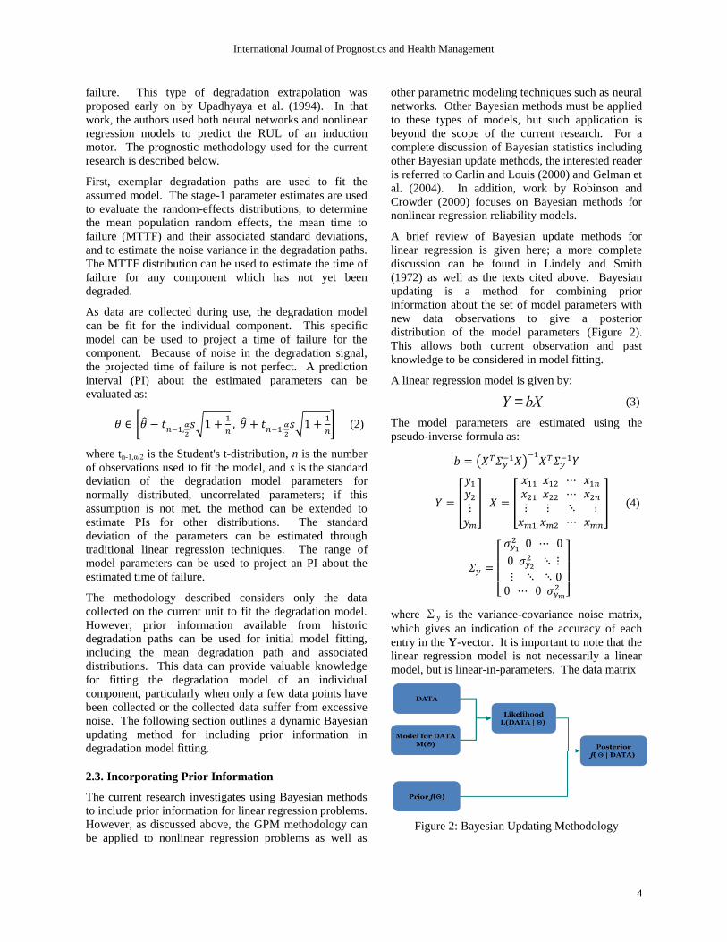
A brief review of Bayesian update methods for

linear regression is given here; a more complete

discussion can be found in Lindely and Smith

(1972) as well as the texts cited above. Bayesian

updating is a method for combining prior

information about the set of model parameters with

new data observations to give a posterior

distribution of the model parameters (Figure 2).

This allows both current observation and past

knowledge to be considered in model fitting.

A linear regression model is given by:

(3)

The model parameters are estimated using the

pseudo-inverse formula as:

(4)

where Σy is the variance-covariance noise matrix,

which gives an indication of the accuracy of each

entry in the Y-vector. It is important to note that the

linear regression model is not necessarily a linear

model, but is linear-in-parameters. The data matrix

Figure 2: Bayesian Updating Methodology

Y = bX


5

X can be populated with any function of degradation

measures, including higher order terms, interaction terms,

and functions such as sin(x) or ex. If prior information is

available for a specific model parameter, i.e. βj~N(βjo,σ2β ), then the matrix X should be appended with an

additional row with value one at the jth

position and zero

elsewhere, and the Y matrix should be appended with the a

priori value of the jth

parameter.

(5)

Finally, the variance-covariance matrix is augmented with

a final row and column of zeros, with the variance of the a

priori information in the diagonal element.

(6)

If knowledge is available about multiple regression

parameters, the matrices should be appended multiple

times with one row for each parameter.

It is convenient to assume that the noise in the degradation

measurements is constant and uncorrelated. Some a priori

knowledge of the noise variance is available from the

exemplar degradation paths. If this assumption is not valid

for a particular system, then other methods of estimating

the noise variance may be used; however, it has been seen

anecdotally that violating this assumption does not have a

significant impact on RUL estimation. In addition, it is

also convenient to assume that the noise measurements are

uncorrelated across observations of y; this allows the

variance-covariance matrix to be a diagonal matrix

consisting of noise variance estimates and a priori

knowledge variance estimates. If this assumption is not

valid, including covariance terms is trivial; again, these

terms can be estimated from historical degradation paths.

After a priori knowledge is used in conjunction with

n current data observations to obtain a posterior

estimate of degradation parameters, this estimate

becomes the new prior distribution for the next

estimation of regression parameters. The variance

of this new knowledge is estimated as:

(7)

The Bayesian information may be used to

dynamically update the model fit as new data

become available for each desired RUL estimate.

2.4. Combined Monitoring and Prognostic

Systems

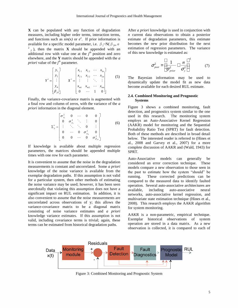
Figure 3 shows a combined monitoring, fault

detection, and prognostics system similar to the one

used in this research. The monitoring system

employs an Auto-Associative Kernel Regression

(AAKR) model for monitoring and the Sequential

Probability Ratio Test (SPRT) for fault detection.

Both of these methods are described in broad detail

below. The interested reader is referred to (Hines et

al., 2008 and Garvey et al., 2007) for a more

complete discussion of AAKR and (Wald, 1943) for

SPRT.

Auto-Associative models can generally be

considered an error correction technique. These

models compare a new observation to those seen in

the past to estimate how the system “should” be

running. These corrected predictions can be

compared to the measured data to identify faulted

operation. Several auto-associative architectures are

available, including auto-associative neural

networks, auto-associative kernel regression, and

multivariate state estimation technique (Hines et al.,

2008). This research employs the AAKR algorithm

for system monitoring.

AAKR is a non-parametric, empirical technique.

Exemplar historical observations of system

operation are stored in a data matrix. As a new

observation is collected, it is compared to each of

Figure 3: Combined Monitoring and Prognostic System

010

21

22 22 1

11 21 1

*

0

2

1

*

mnmm

n

n

j

m xxx

xxx

xxx

X

y

y

y

Y

2

2

2

2

*

0

2

1

000

000

0

00

000

j

my

y

y

y

s post

2 =1

s prior

2+

n

s y

2

æ

è ç ç

ö

ø ÷ ÷

-1

6

the exemplar observations to determine how similar the

new observation is to each of the exemplars. This

similarity is quantified by evaluating the distance between

the new observation and the exemplar. Most commonly,

the Euclidean distance is used:

di = X j - x i, j( )2

j=1

m

å (8)

where di is the distance between the new observation, X,

and the ith

exemplar, xi. The distance is converted to a

similarity measure through the use of a kernel. Many

kernels are available; this research employs the Gaussian

kernel:

(9)

where si is the similarity of the new observation to the ith

exemplar and h is the kernel bandwidth, which controls

how close vectors must be to be considered similar.

Finally, the “corrected” observation value is calculated as

a weighted average of the exemplar observations:

(10)

Monitoring system residuals are then generated as the

difference between the actual observation and the error-

corrected prediction. These residuals are used with a

SPRT to determine if the system is operating in a faulted

or nominal condition. As the name suggests, the SPRT

looks at a sequence of residuals to determine if the time

series of data is more likely from a nominal distribution or

a pre-specified faulted distribution. As new observations

are made, the SPRT compares the cumulative sum of the

log-likelihood ratio:

(11)

to two thresholds, which depend on the acceptable false

positive and false negative fault rates:

(12)

where is the acceptable false alarm (false positive) rate

and is the acceptable missed alarm (false negative) rate.

For this research, false alarm and missed alarm rates of 1%

and 10% respectively are used. If si < a, then the null

hypothesis cannot be rejected; that is, the system is

assumed to be operating in a nominal condition. If si > b,

then the null hypothesis is rejected; that is, the

system is assumed to be operating in a faulted

condition. When a determination is made, the sum,

si, is reset to zero and the test is restarted.

After a fault is detected in the system, the prognostic

system can be engaged to determine the RUL for the

system. As discussed above, the GPM methodology

uses a measure of system degradation, called a

prognostic parameter, to make prognostic estimates.

An ideal prognostic parameter has three key

qualities: monotonicity, prognosability, and

trendability.

Monotonicity characterizes the underlying positive

or negative trend of the parameter. This is an

important feature of a prognostic parameter because

it is generally assumed that systems do not undergo

self-healing, which would be indicated by a non-

monotonic parameter. This assumption is not valid

for some components such as batteries, which may

experience some degree of self repair during short

periods of nonuse, but it tends to hold for

mechanical systems or for complex systems as a

whole.

Prognosability gives a measure of the variance in the

critical failure value of a population of systems. A

wide spread in critical failure values can make it

difficult to accurately define a critical failure

threshold and to extrapolate a prognostic parameter

to failure. Prognosability may be very susceptible to

noise in the prognostic parameter, but this effect

may be reduced by traditional variance reduction

methods such as parameter bagging and data

denoising.

Finally, trendability indicates the degree to which

the parameters of a population of systems have the

same underlying shape and can be described by the

same functional form.

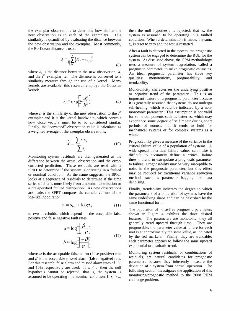
The population of noise-free prognostic parameters

shown in Figure 4 exhibits the three desired

features. The parameters are monotonic: they all

generally trend upward through time. They are

prognosable: the parameter value at failure for each

unit is at approximately the same value, as indicated

by the red markers. Finally, they are trendable:

each parameter appears to follow the same upward

exponential or quadratic trend.

Monitoring system residuals, or combinations of

residuals, are natural candidates for prognostic

parameters because they inherently measure the

deviation of a system from normal operation. The

following section investigates the application of this

monitoring/prognostic method to the 2008 PHM

challenge problem.

si = exp -di

2

h2

æ

è ç

ö

ø ÷

ˆ X =six iåsiå

iii ss lo g1

a » logb

1-a

æ

è ç

ö

ø ÷

b » log1- b

a

æ

è ç

ö

ø ÷


7

Figure 4: Population of "good" prognostic parameters

3. PHM ’08 CHALLENGE APPLICATION

This section presents an application of the proposed GPM

prognostic method to the PHM Challenge data set. The

efficacy of the method is analyzed based on the given cost

function for the 218 test cases. RUL estimates far from

the actual value are penalized exponentially. The cost

function is asymmetric; RUL predictions greater than the

actual value are penalized more heavily than those which

predict failure before it happens. The cost for each case is

given by the following formula:

(13)

where d is the difference between the estimated and the

actual RUL. If d is negative, then the algorithm

underestimates the RUL leading one to end operation

before failure occurs; if d is positive, then the algorithm

overestimates the RUL and results in a greater penalty

because one may attempt to operate the component longer

than possible and thereby experience a failure. The

following sections give a brief description of the simulated

data set used for the challenge problem, then outline the

data analysis and identification of an appropriate

prognostic parameter for GPM trending. Finally, the

application of the GPM method and Bayesian updating are

presented with final results given for the described

method. The performance of the GPM algorithm with and

without Bayesian updating is compared.

3.1. PHM Challenge Data Set Description

The PHM Challenge data set consists of 218 cases of

multivariate data that track from nominal operation

through fault onset to system failure. Data were provided

which modeled the damage propagation of aircraft gas

turbine engines using the Commercial Modular Aerop-

Propulsion System Simulation (C-MAPSS). This engine

simulator allows faults to be injected in any of the

five rotating components and gives output responses

for 58 sensed engine variables. The PHM Challenge

data set included 21 of these 58 output variables as

well as three operating condition indicators. Each

simulated engine was given some initial level of

wear which would be considered within normal

limits, and faults were initiated at some random time

during the simulation. Fault propagation was

assumed to evolve in an exponential way based on

common fault propagation models and the results

seen in practice. Engine health was determined as

the minimum health margin of the rotating

equipment, where the health margin was a function

of efficiency and flow for that particular component;

when this health indicator reached zero, the

simulated engine was considered failed. The

interested reader is referred to Saxena et al. (2008)

for a more complete description of the data

simulation.

The data have three operational variables – altitude,

Mach number, and TRA – and 21 sensor

measurements. Initial data analysis resulted in the

identification of six distinct operational settings;

based on this result, the operating condition

indicators were collapsed into one indicator which

fully defined the operating condition of the engine

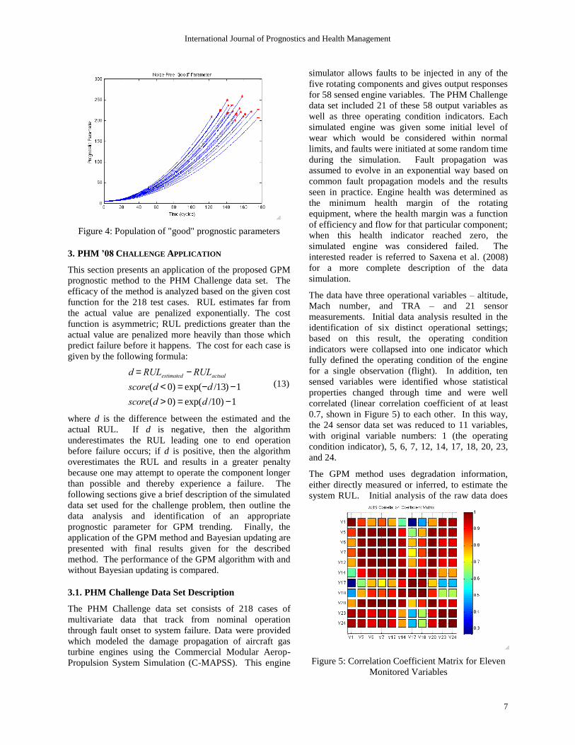
for a single observation (flight). In addition, ten

sensed variables were identified whose statistical

properties changed through time and were well

correlated (linear correlation coefficient of at least

0.7, shown in Figure 5) to each other. In this way,

the 24 sensor data set was reduced to 11 variables,

with original variable numbers: 1 (the operating

condition indicator), 5, 6, 7, 12, 14, 17, 18, 20, 23,

and 24.

The GPM method uses degradation information,

either directly measured or inferred, to estimate the

system RUL. Initial analysis of the raw data does

Figure 5: Correlation Coefficient Matrix for Eleven

Monitored Variables

d = RULestimated - RULactual

score(d < 0) = exp(-d /13) -1

score(d > 0) = exp(d /10) -1


8

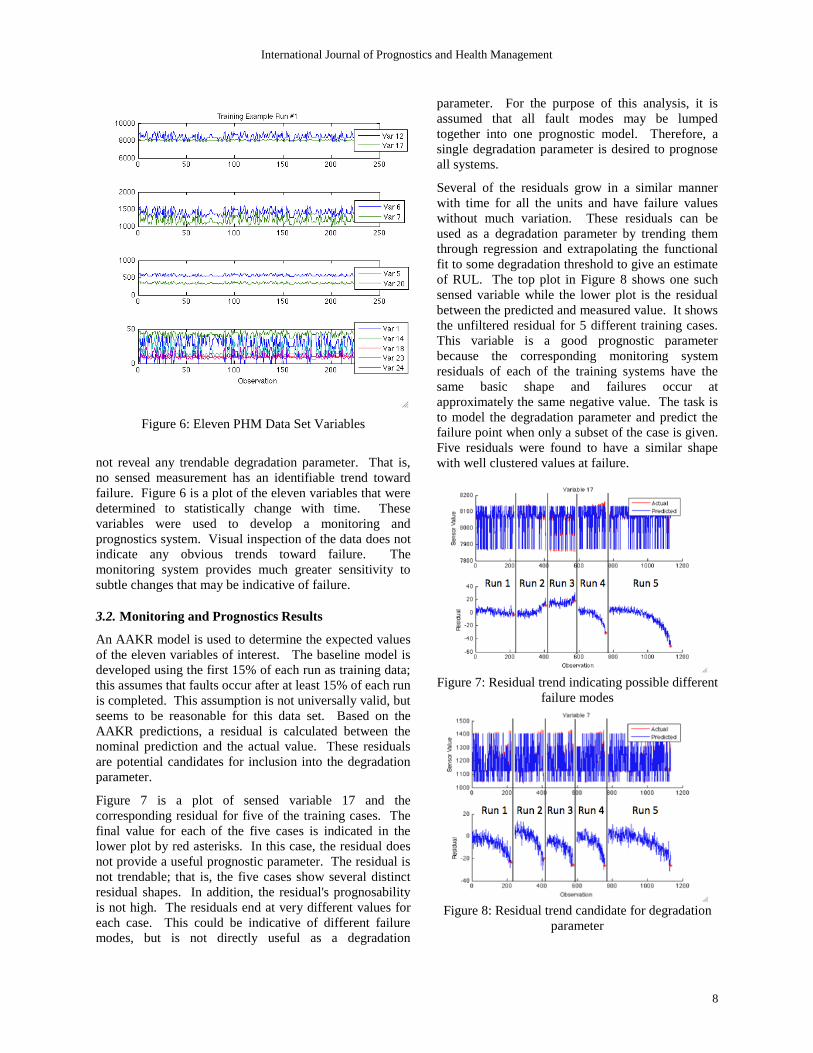
Figure 6: Eleven PHM Data Set Variables

not reveal any trendable degradation parameter. That is,

no sensed measurement has an identifiable trend toward

failure. Figure 6 is a plot of the eleven variables that were

determined to statistically change with time. These

variables were used to develop a monitoring and

prognostics system. Visual inspection of the data does not

indicate any obvious trends toward failure. The

monitoring system provides much greater sensitivity to

subtle changes that may be indicative of failure.

3.2. Monitoring and Prognostics Results

An AAKR model is used to determine the expected values

of the eleven variables of interest. The baseline model is

developed using the first 15% of each run as training data;

this assumes that faults occur after at least 15% of each run

is completed. This assumption is not universally valid, but

seems to be reasonable for this data set. Based on the

AAKR predictions, a residual is calculated between the

nominal prediction and the actual value. These residuals

are potential candidates for inclusion into the degradation

parameter.

Figure 7 is a plot of sensed variable 17 and the

corresponding residual for five of the training cases. The

final value for each of the five cases is indicated in the

lower plot by red asterisks. In this case, the residual does

not provide a useful prognostic parameter. The residual is

not trendable; that is, the five cases show several distinct

residual shapes. In addition, the residual's prognosability

is not high. The residuals end at very different values for

each case. This could be indicative of different failure

modes, but is not directly useful as a degradation

parameter. For the purpose of this analysis, it is

assumed that all fault modes may be lumped

together into one prognostic model. Therefore, a

single degradation parameter is desired to prognose

all systems.

Several of the residuals grow in a similar manner

with time for all the units and have failure values

without much variation. These residuals can be

used as a degradation parameter by trending them

through regression and extrapolating the functional

fit to some degradation threshold to give an estimate

of RUL. The top plot in Figure 8 shows one such

sensed variable while the lower plot is the residual

between the predicted and measured value. It shows

the unfiltered residual for 5 different training cases.

This variable is a good prognostic parameter

because the corresponding monitoring system

residuals of each of the training systems have the

same basic shape and failures occur at

approximately the same negative value. The task is

to model the degradation parameter and predict the

failure point when only a subset of the case is given.

Five residuals were found to have a similar shape

with well clustered values at failure.

Figure 7: Residual trend indicating possible different

failure modes

Figure 8: Residual trend candidate for degradation

parameter


9

By combining the five degradation parameters with similar

shapes, an average parameter was developed. The five

residuals are combined in a weighted average, where each

residual weight is inversely proportional to its variance.

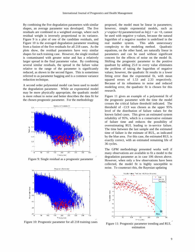
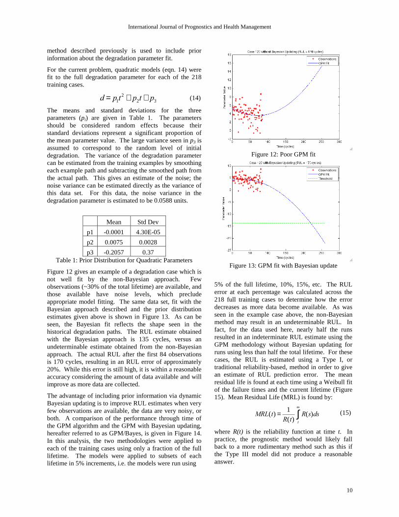
Figure 9 is a plot of one of the candidate residuals, and

Figure 10 is the averaged degradation parameter resulting

from a fusion of the five residuals for all 218 cases. As the

plots show, the residual parameters have very similar

shapes for each training case. However, the single residual

is contaminated with greater noise and has a relatively

larger spread in the final parameter value. By combining

several similar residuals, the spread in the failure value

relative to the range of the parameter is significantly

reduced, as shown in the second figure. This is sometimes

referred to as parameter bagging and is a common variance

reduction technique.

A second order polynomial model can been used to model

the degradation parameter. While an exponential model

may be more physically appropriate, the quadratic model

is more robust to noise and better describes the data fit for

the chosen prognostic parameter. For the methodology

Figure 9: Single residual as a prognostic parameter

Figure 10: Prognostic parameter for all 218 training cases

proposed, the model must be linear in parameters;

however, simple exponential models, such as

y=exp(ax+b) parameterized as ln(y) = ax +b, cannot

be used with negative y-values, because the natural

logarithm of a negative number is undefined in the

real number system. This adds unnecessary

complexity to the modeling method. Quadratic

equations, on the other hand, are naturally linear in

parameters and can be used without significant

concern for the effects of noise on the model fit.

Shifting the prognostic parameter to the positive

quadrant by adding 25.0 to every value eliminates

the problem of taking the logarithm of negative

values; however, the quadratic fit results in a lower

fitting error than the exponential fit, with mean

squared errors of 1.53 and 2.33 respectively.

Because of its robustness to noise and reduced

modeling error, the quadratic fit is chosen for this

research.

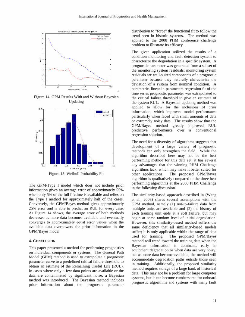
Figure 11 gives an example of a polynomial fit of

the prognostic parameter with the time the model

crosses the critical failure threshold indicated. The

threshold of -13.9 was chosen as the upper 95%

level of the distribution of failure values for the

known failed cases. This gives an estimated system

reliability of 95%, which is a conservative estimate

of failure time and reduces the possibility of

overestimating RUL leading to in-service failure.

The time between the last sample and the estimated

time of failure is the estimate of RUL, as indicated

by the blue area. For this case, the estimated RUL is

exactly correct, with an estimated remaining life of

36 cycles.

The GPM methodology presented works well if

many observations are available to fit a model to the

degradation parameter as in case 106 shown above.

However, when only a few observations have been

collected, the model fit is highly susceptible to

noise. To counteract this, the Bayesian updating

Figure 11: Prognostic parameter trending and RUL

estimation


10

method described previously is used to include prior

information about the degradation parameter fit.

For the current problem, quadratic models (eqn. 14) were

fit to the full degradation parameter for each of the 218

training cases.

(14)

The means and standard deviations for the three

parameters (pi) are given in Table 1. The parameters

should be considered random effects because their

standard deviations represent a significant proportion of

the mean parameter value. The large variance seen in p3 is

assumed to correspond to the random level of initial

degradation. The variance of the degradation parameter

can be estimated from the training examples by smoothing

each example path and subtracting the smoothed path from

the actual path. This gives an estimate of the noise; the

noise variance can be estimated directly as the variance of

this data set. For this data, the noise variance in the

degradation parameter is estimated to be 0.0588 units.

Mean Std Dev

p1 -0.0001 4.30E-05

p2 0.0075 0.0028

p3 -0.2057 0.37

Table 1: Prior Distribution for Quadratic Parameters

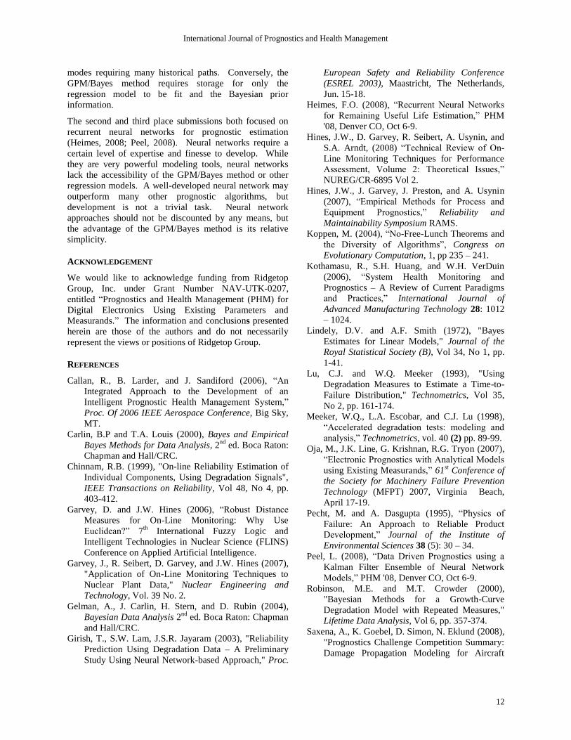
Figure 12 gives an example of a degradation case which is

not well fit by the non-Bayesian approach. Few

observations (~30% of the total lifetime) are available, and

those available have noise levels, which preclude

appropriate model fitting. The same data set, fit with the

Bayesian approach described and the prior distribution

estimates given above is shown in Figure 13. As can be

seen, the Bayesian fit reflects the shape seen in the

historical degradation paths. The RUL estimate obtained

with the Bayesian approach is 135 cycles, versus an

undeterminable estimate obtained from the non-Bayesian

approach. The actual RUL after the first 84 observations

is 170 cycles, resulting in an RUL error of approximately

20%. While this error is still high, it is within a reasonable

accuracy considering the amount of data available and will

improve as more data are collected.

The advantage of including prior information via dynamic

Bayesian updating is to improve RUL estimates when very

few observations are available, the data are very noisy, or

both. A comparison of the performance through time of

the GPM algorithm and the GPM with Bayesian updating,

hereafter referred to as GPM/Bayes, is given in Figure 14.

In this analysis, the two methodologies were applied to

each of the training cases using only a fraction of the full

lifetime. The models were applied to subsets of each

lifetime in 5% increments, i.e. the models were run using

Figure 12: Poor GPM fit

Figure 13: GPM fit with Bayesian update

5% of the full lifetime, 10%, 15%, etc. The RUL

error at each percentage was calculated across the

218 full training cases to determine how the error

decreases as more data become available. As was

seen in the example case above, the non-Bayesian

method may result in an undeterminable RUL. In

fact, for the data used here, nearly half the runs

resulted in an indeterminate RUL estimate using the

GPM methodology without Bayesian updating for

runs using less than half the total lifetime. For these

cases, the RUL is estimated using a Type I, or

traditional reliability-based, method in order to give

an estimate of RUL prediction error. The mean

residual life is found at each time using a Weibull fit

of the failure times and the current lifetime (Figure

15). Mean Residual Life (MRL) is found by:

(15)

where R(t) is the reliability function at time t. In

practice, the prognostic method would likely fall

back to a more rudimentary method such as this if

the Type III model did not produce a reasonable

answer.

d = p1t2 + p2t + p3

MRL(t) =1

R(t)R(s)ds

t

¥

ò


11

Figure 14: GPM Results With and Without Bayesian

Updating

Figure 15: Weibull Probability Fit

The GPM/Type I model which does not include prior

information gives an average error of approximately 55%

when only 5% of the full lifetime is available and relies on

the Type I method for approximately half of the cases.

Conversely, the GPM/Bayes method gives approximately

25% error and is able to predict an RUL for every case.

As Figure 14 shows, the average error of both methods

decreases as more data becomes available and eventually

converges to approximately equal error values when the

available data overpowers the prior information in the

GPM/Bayes model.

4. CONCLUSION

This paper presented a method for performing prognostics

on individual components or systems. The General Path

Model (GPM) method is used to extrapolate a prognostic

parameter curve to a predefined critical failure threshold to

obtain an estimate of the Remaining Useful Life (RUL).

In cases where only a few data points are available or the

data are contaminated by significant noise, a Bayesian

method was introduced. The Bayesian method includes

prior information about the prognostic parameter

distribution to "force" the functional fit to follow the

trend seen in historic systems. The method was

applied to the 2008 PHM conference challenge

problem to illustrate its efficacy.

The given application utilized the results of a

condition monitoring and fault detection system to

characterize the degradation in a specific system. A

prognostic parameter was generated from a subset of

the monitoring system residuals; monitoring system

residuals are well-suited components of a prognostic

parameter because they naturally characterize the

deviation of a system from nominal condition. A

parametric, linear-in-parameters regression fit of the

time series prognostic parameter was extrapolated to

the critical failure threshold to give an estimate of

the system RUL. A Bayesian updating method was

applied to allow for the inclusions of prior

information, which improves model performance

particularly when faced with small amounts of data

or extremely noisy data. The results show that the

GPM/Bayes method greatly improved RUL

predictive performance over a conventional

regression solution.

The need for a diversity of algorithms suggests that

development of a large variety of prognostic

methods can only strengthen the field. While the

algorithm described here may not be the best

performing method for this data set, it has several

key advantages that the winning PHM Challenge

algorithms lack, which may make it better suited for

other applications. The proposed GPM/Bayes

algorithm is qualitatively compared to the three best

performing algorithms at the 2008 PHM Challenge

in the following discussion.

The similarity-based approach described in (Wang

et al., 2008) shares several assumptions with the

GPM method, namely (1) run-to-failure data from

multiple units are available and (2) the history of

each training unit ends at a soft failure, but may

begin at some random level of initial degradation.

However, this similarity-based method suffers the

same deficiency that all similarity-based models

suffer; it is only applicable within the range of data

used for training. The proposed GPM/Bayes

method will trend toward the training data when the

Bayesian information is dominant, early in

equipment degradation or when data are very noisy,

but as more data become available, the method will

accommodate degradation paths outside those seen

in training. Additionally, the proposed similarity

method requires storage of a large bank of historical

data. This may not be a problem for large computer

systems, but it can become cumbersome for onboard

prognostic algorithms and systems with many fault


12

modes requiring many historical paths. Conversely, the

GPM/Bayes method requires storage for only the

regression model to be fit and the Bayesian prior

information.

The second and third place submissions both focused on

recurrent neural networks for prognostic estimation

(Heimes, 2008; Peel, 2008). Neural networks require a

certain level of expertise and finesse to develop. While

they are very powerful modeling tools, neural networks

lack the accessibility of the GPM/Bayes method or other

regression models. A well-developed neural network may

outperform many other prognostic algorithms, but

development is not a trivial task. Neural network

approaches should not be discounted by any means, but

the advantage of the GPM/Bayes method is its relative

simplicity.

ACKNOWLEDGEMENT

We would like to acknowledge funding from Ridgetop

Group, Inc. under Grant Number NAV-UTK-0207,

entitled “Prognostics and Health Management (PHM) for

Digital Electronics Using Existing Parameters and

Measurands.” The information and conclusions presented

herein are those of the authors and do not necessarily

represent the views or positions of Ridgetop Group.

REFERENCES

Callan, R., B. Larder, and J. Sandiford (2006), “An

Integrated Approach to the Development of an

Intelligent Prognostic Health Management System,”

Proc. Of 2006 IEEE Aerospace Conference, Big Sky,

MT.

Carlin, B.P and T.A. Louis (2000), Bayes and Empirical

Bayes Methods for Data Analysis, 2nd

ed. Boca Raton:

Chapman and Hall/CRC.

Chinnam, R.B. (1999), "On-line Reliability Estimation of

Individual Components, Using Degradation Signals",

IEEE Transactions on Reliability, Vol 48, No 4, pp.

403-412.

Garvey, D. and J.W. Hines (2006), “Robust Distance

Measures for On-Line Monitoring: Why Use

Euclidean?” 7th

International Fuzzy Logic and

Intelligent Technologies in Nuclear Science (FLINS)

Conference on Applied Artificial Intelligence.

Garvey, J., R. Seibert, D. Garvey, and J.W. Hines (2007),

"Application of On-Line Monitoring Techniques to

Nuclear Plant Data," Nuclear Engineering and

Technology, Vol. 39 No. 2.

Gelman, A., J. Carlin, H. Stern, and D. Rubin (2004),

Bayesian Data Analysis 2nd

ed. Boca Raton: Chapman

and Hall/CRC.

Girish, T., S.W. Lam, J.S.R. Jayaram (2003), "Reliability

Prediction Using Degradation Data – A Preliminary

Study Using Neural Network-based Approach," Proc.

European Safety and Reliability Conference

(ESREL 2003), Maastricht, The Netherlands,

Jun. 15-18.

Heimes, F.O. (2008), “Recurrent Neural Networks

for Remaining Useful Life Estimation,” PHM

'08, Denver CO, Oct 6-9.

Hines, J.W., D. Garvey, R. Seibert, A. Usynin, and

S.A. Arndt, (2008) “Technical Review of On-

Line Monitoring Techniques for Performance

Assessment, Volume 2: Theoretical Issues,”

NUREG/CR-6895 Vol 2.

Hines, J.W., J. Garvey, J. Preston, and A. Usynin

(2007), “Empirical Methods for Process and

Equipment Prognostics,” Reliability and

Maintainability Symposium RAMS.

Koppen, M. (2004), “No-Free-Lunch Theorems and

the Diversity of Algorithms”, Congress on

Evolutionary Computation, 1, pp 235 – 241.

Kothamasu, R., S.H. Huang, and W.H. VerDuin

(2006), “System Health Monitoring and

Prognostics – A Review of Current Paradigms

and Practices,” International Journal of

Advanced Manufacturing Technology 28: 1012

– 1024.

Lindely, D.V. and A.F. Smith (1972), "Bayes

Estimates for Linear Models," Journal of the

Royal Statistical Society (B), Vol 34, No 1, pp.

1-41.

Lu, C.J. and W.Q. Meeker (1993), "Using

Degradation Measures to Estimate a Time-to-

Failure Distribution," Technometrics, Vol 35,

No 2, pp. 161-174.

Meeker, W.Q., L.A. Escobar, and C.J. Lu (1998),

“Accelerated degradation tests: modeling and

analysis,” Technometrics, vol. 40 (2) pp. 89-99.

Oja, M., J.K. Line, G. Krishnan, R.G. Tryon (2007),

“Electronic Prognostics with Analytical Models

using Existing Measurands,” 61st Conference of

the Society for Machinery Failure Prevention

Technology (MFPT) 2007, Virginia Beach,

April 17-19.

Pecht, M. and A. Dasgupta (1995), “Physics of

Failure: An Approach to Reliable Product

Development,” Journal of the Institute of

Environmental Sciences 38 (5): 30 – 34.

Peel, L. (2008), “Data Driven Prognostics using a

Kalman Filter Ensemble of Neural Network

Models,” PHM '08, Denver CO, Oct 6-9.

Robinson, M.E. and M.T. Crowder (2000),

"Bayesian Methods for a Growth-Curve

Degradation Model with Repeated Measures,"

Lifetime Data Analysis, Vol 6, pp. 357-374.

Saxena, A., K. Goebel, D. Simon, N. Eklund (2008),

"Prognostics Challenge Competition Summary:

Damage Propagation Modeling for Aircraft


13

Engine Run-to-Failure Simulation," PHM '08, Denver

CO, Oct 6-9.

Upadhyaya, B.R., M. Naghedolfeizi, and B. Raychaudhuri

(1994), "Residual Life Estimation of Plant

Components," P/PM Technology, June, pp. 22-29.

Valentin, R., M. Osterman, B. Newman (2003),

“Remaining Life Assessment of Aging Electronics in

Avionic Applications,” 2003 Proceedings of the

Annual Reliability and Maintainability Symposium

(RAMS): 313 – 318.

Wald, A. (1945), “Sequential Tests of Statistical

Hypotheses,” The Annals of Mathematical Statistics

June 1945, vol. 16 (2) pp. 117-186.

Wang, P. and D.W. Coit (2004), "Reliability Prediction

based on Degradation Modeling for Systems with

Multiple Degradation Measures," Proc. of the 2004

Reliability and Maintainability Symposium, pp. 302-

307.

Wang,T. J. Yu, D. Seigel, and J. Lee (2008), “A

Similarity-Based Prognostics Approach for

Remaining Useful Life Estimation of Engineered

Systems,” PHM '08, Denver CO, Oct 6-9.

Dr. Jamie B. Coble attended the University of Tennessee,

Knoxville where she graduated Summa Cum Laude with a

Bachelor of Science degree in both Nuclear Engineering

and Mathematics and a minor in Engineering

Communication and Performance in May, 2005. She also

completed the University Honors Program with a Senior

Project titled, "Investigating Neutron Spectra Changes in

Deep Penetration Shielding Analyses." In January, 2005,

she began work with Dr. Mario Fontana investigating the

effects of long-term station blackouts on boiling water

reactors, focusing particularly on the radionuclide release

to the environment. In October, 2005, she began research

with Dr. J. Wesley Hines investigating the effects of poor

model construction on auto-associative model

architectures for on-line monitoring systems. This work

was incorporated into the final volume of a NUREG series

for the U.S. Nuclear Regulatory Commission (NRC).

She received an MS in Nuclear Engineering for this

work in August, 2006. She was the first graduate of

the Reliability and Maintenance Engineering MS

program in August, 2009. She completed her Ph.D.

in Nuclear Engineering in May, 2010 with work

focusing on automated methods for identifying

appropriate prognostic parameters for use in

individual-based prognosis. Her current research is

in the area of empirical methods for system

monitoring, fault detection and isolation, and

prognostics. She is a member of the engineering

honors society Tau Beta Pi, the national honors

society Omicron Delta Kappa, the Institute for

Electrical and Electronics Engineers Reliability

Society, and the American Nuclear Society.

Dr. J. Wesley Hines is a Professor of Nuclear

Engineering at the University of Tennessee and is

the director of the Reliability and Maintainability

Engineering Education program. He received the

BS degree in Electrical Engineering from Ohio

University in 1985, and then was a nuclear qualified

submarine officer in the Navy. He received both an

MBA and an MS in Nuclear Engineering from The

Ohio State University in 1992, and a Ph.D. in

Nuclear Engineering from The Ohio State

University in 1994. Dr. Hines teaches and conducts

research in artificial intelligence and advanced

statistical techniques applied to process diagnostics,

condition based maintenance, and prognostics.

Much of his research program involves the

development of algorithms and methods to monitor

high value equipment, detect abnormalities, and

predict time to failure. He has authored over 250

papers and has several patents in the area of

advanced process monitoring and prognostics

techniques. He is a director of the Prognostics and

Health Management Society, and a member of the

American Nuclear Society, American Society of

Engineering Education.

Documents

Applying the General Path Model to Estimation of Remaining Useful · PDF fileApplying the General Path Model to Estimation of Remaining Useful Life Jamie Coble1 and J. Wesley Hines2