Learning the Master's Trade: Apprenticeship and

Human Capital in Ghana§

Garth Frazer†

Centre for Industrial Relations, University of Toronto, 121 St. George Street, Toronto, ON, Canada M5S 2E8

School of Management, University of Toronto, 105 St. George Street, Toronto, ON, Canada M5S 3E6

Abstract This paper explores the institution of apprenticeship in Ghana. A model is presented where

apprenticeship training is idiosyncratic, increasing an individual's productivity in the current

firm, but not in any other firm. Still, individuals are willing to fund apprenticeships as they

can reap the returns to the specific training of apprenticeship if they manage to acquire the

capital required to start their own firms, and replicate the technology and business practice

of the apprenticeship firm. Predictions of the model for the productivity and remuneration of

different workers are developed and tested using both a linked employer-employee survey of

manufacturing firms, and a national household survey.

JEL Codes: O12, J23, J24

keywords: apprenticeship, Africa, human capital

§ This work has benefited from the very useful comments and suggestions of two anonymous referees and the Editor, as well as Christopher Udry, David McKenzie, Patrick Bayer, and seminar participants at the University of British Columbia, Northwestern University, Yale University, Stanford University, and Carleton University. Financial support from the Connaught Fund is gratefully acknowledged. Permission from the Ghana Statistical Service to use the Ghanaian Living Standard Survey data is most certainly appreciated. The author owes a particular debt to Francis Teal for the opportunity to participate in the Ghanaian Manufacturing Enterprise Survey, and for the use of its data. † Tel: +1 416 978 5692, Fax: +1 416 978 5433. E-mail address: gfrazer@chass.utoronto.ca

1 Introduction

The formulation of an appropriate education and training policy for the manufacturing

sector in Africa should begin with an understanding of the training currently in place.

Given the importance of apprenticeships in Africa,1 where apprentices learn one of the

trades used in the manufacturing sector, any analysis should begin by examining this

institution. Nevertheless, very few articles exist which use economic analysis to explore

apprenticeships in Africa (Velenchik, 1995). This paper is a step towards addressing this

dearth, and contends that the apprenticeship institution is best understood in the larger

context of the specificity of firm training.

Apprenticeships are periods of roughly three years in length during which an

apprentice learns a trade, such as metal-working or carpentry from a master of that trade.

At the end of the apprenticeship, the apprentice may end up being hired by the firm where

the apprenticeship occurred, begin working at another firm, or the apprentice may start a

new firm and become self-employed. Apprenticeships occur most often, but not

exclusively, in smaller firms, and the master is often the owner of the firm.

Becker (1964) showed that in the human capital model with perfect labor markets,

workers (and not firms) always pay for general training, which increases an individual’s

productivity with all employers, as the value of their outside wage offer increases with

general training. However, firms cannot credibly commit, without some formal contracting

or other mechanism, to compensate workers for firm-specific training once it has occurred,

as it does not increase their outside wage offers. This dichotomy has provided a framework

1Apprenticeships are particularly important in West Africa, but are significant institutions throughoutAfrica. Their significance is documented in Boehm (1997) and Bas (1989).

1

for analyzing the nature of training in a number of studies. Acemoglu and Pischke (1998)

treat German apprenticeships as general training, and present a model that explains why

firms are willing to invest in this training. Acemoglu (1997) and Acemoglu and Pischke

(1999) provide distinct models which explain why firms might invest in general training.

Other papers have examined worker investment in firm-specific training.

Prendergast (1993) describes the potential for promotion rules to induce worker

investments in firm-specific human capital, with the firm’s ability to commit to future wage

increases through long-term contracts playing a significant role in the model’s mechanism.

Scoones and Bernhardt (1998) remove the need for long-term contracts to achieve worker

investment in firm-specific human capital by introducing asymmetric information. In their

model, workers invest in firm-specific human capital, in order to be promoted by the firm,

as promotion reveals their higher ability to other firms. In a similar model, Scoones (2000)

finds that workers invest in firm-specific capital because efficient turnover transforms

former employers into outside options. Other papers (e.g. Felli and Harris, 1994) examine

firm-specific human capital as something exogenous to worker decisions, but we are

interested in examining investment in human capital that is discretionary from the worker

perspective.

At first glance, apprenticeships might appear to be general training, that is

applicable at least in all of the firms within an industry, if not more generally. As noted,

this is how they have been understood in Germany. However, the nature of the training

acquired in Ghana is far more specific—specific to the firm providing the training, reflecting

the firm’s technology and business practice. In this context, the model of apprenticeship

to be developed shares the spirit of the model of Jovanovic and Nyarko (1995). In their

2

overlapping generations model, each old agent understands an idiosyncratic (which is

unique to the firm owned by the old agent) technology which is passed on to a young agent

who is his apprentice. This interpretation of apprenticeships as training unique to the firm

is consistent with the apprenticeships under examination in this paper.2 Apprentices are

taught by a master how to work the master’s craft, but the way in which that craft is

carried out varies highly from firm to firm. In the process of this research investigation, I

visited and interviewed dozens of the manufacturing firms in the dataset. A number of the

firms interviewed were involved in the manufacture of a single item. When apprentices

apprentice at these firms, they may only learn how to manufacture one, or a small number

of items. While apprentices at other firms did learn how to manufacture a wider variety of

items, product homogeneity, using unique technology, is quite common among the practice

of firms with apprentices. The training given by the master, both in terms of technology

and business practice, is that of the master, and typically idiosyncratic.3

Therefore, the apprenticeship training cannot be applied to work in other firms,

which have their own technology and business practice. However, once the apprenticeship

is complete, the former apprentice can use this knowledge to start his own firm and pursue

self-employment, replicating the apprenticeship firm. In fact, apprentices appear highly

motivated to pursue self-employment. Of the Ghanaian manufacturing workers, who had

completed apprenticeships, 77% stated that they would prefer to be self-employed rather

2The apprenticeships under examination in this paper include all of the non-tailoring apprenticeships inGhana, in particular those within the Ghanaian manufacturing sector. Tailoring apprenticeships are to beconsidered in a separate paper by the same author in order to account for their idiosyncratic nature.

3The idiosyncratic nature of the technologies used by apprenticeship in Ghana relates to a larger literatureon the technological capabilities within African countries. Lall and Pietrobelli (2002) explore the roots ofthe limited technological capabilities within Africa in much greater depth than is possible here. Lall et. al.(1994) focus on technological capabilities in manufacturing (and the limitations thereof) in the particularcontext of Ghana.

3

than working in their current job. Naturally, however, apprenticeship knowledge is not

enough—capital is required to start a firm. Those former apprentices who get access to

capital can start a new firm, while others cannot. The potential to reap the returns of the

apprenticeship, this specific training, by creating a new firm and replicating the technology

and business practice of the apprenticeship firm motivates individuals to acquire the

human capital of apprenticeship.

This apprenticeship human capital is not transferable to any other firm outside the

current firm, but it can be used when the apprentice replicates the technology and business

practice of the current firm in self-employment. Therefore, while the apprenticeship

certainly does not provide general human capital (which is useful in all firms), the human

capital is also not ‘firm-specific’ in the pure definition of the term. The human capital can

be used outside of the current firm, but only when the apprentice replicates the

apprenticeship firm. Perhaps a term such as ‘technology-specific’ might better describe the

nature of the apprenticeship human capital. However, this technology should be

understood as unique to the firm providing the apprenticeship training. The exact

labelling of the human capital is not as important as understanding its nature. Therefore,

it shall be called simply ‘specific human capital’ in this paper. Workers are willing to

invest in this type of specific human capital, which is tightly tied to the firm providing

apprenticeship training, not because of asymmetric information, or any other labor market

imperfection, or the firm’s ability to commit to future wage increases, but rather through a

worker’s potential ability to reap the benefits of the apprenticeship through

self-employment.

Of course, once the apprenticeship is finished, the apprentice can also continue to

4

work in the master’s firm. While the apprenticeship knowledge is certainly applicable in

this context, the master, and not the apprentice, reaps the returns to this knowledge. The

reason for this is the fact that while the former apprentice is more productive in the

master’s firm, he is not more productive in other firms, and so his outside wage option is

low. The master, therefore, only needs to pay the former apprentice marginally above his

outside wage option in order to retain him in the firm. Only in self-employment will the

former apprentice receive his full marginal product (including the apprenticeship-enhanced

productivity) as a wage.

Fortunately, this model, which will be formalized in Section 3, creates predictions

which can be tested using the data. Although the model explains worker investment in

specific training, the mechanics of the model resemble Acemoglu and Pischke (1998). The

predictions of the model include the following. Former apprentices who apprenticed in the

current firm should be more productive than former apprentices from other firms.

However, they do not need to be paid more than former apprentices from other firms. For

this reason, former apprentices will seek self-employment, and the returns to apprenticeship

should be found in self-employment. This model shares similarities and differences with

Becker(1964)’s original work in this area. In Becker’s model, workers and firms share the

cost of firm-specific training, although the relative proportions contributed may vary.

Here, we will see that either workers or firms or both may cover the cost of the training,

depending on the market for apprenticeship. In Becker’s model, after the training, firms

pay these specifically-trained workers less than their marginal product. This fact reflects

the firm’s ownership of the worker’s specific capital, and allows the firm to recoup its

portion of the training cost. Here, also, specifically-trained workers receive less than their

5

marginal products in the training firms as a wage. As in Becker’s model, workers with

specific training in a different firm will receive their marginal product in the current firm,

but this amount is less than what their marginal product would have been in their training

firm. While Becker (1964)’s discussion of self-employment is implicit rather than explicit,

an application of the original Becker framework to include self-employment (without credit

constraints, as in the original Becker model) would also see returns to specific training in

self-employment, as the worker becomes owner of his or her specific capital. In fact, one

purpose of this paper is to explicitly and formally make this extrapolation—to examine the

case of specific capital and self-employment, in the context of apprenticeship in Ghana.

An important characteristic of the model is the fact that firms are not allowed to

make time-inconsistent wage offers. That is, in any given period, it will only prove optimal

for firms to pay workers their outside option. As will be outlined in the paper, this reflects

the difficulties in contract enforcement in Africa, through firm reputation or other means.

For comparison purposes, the model for the case of completely enforceable long-term wage

contracts will also be provided. Firms make less profit in the absence of full contract

enforcement, and a measure of this loss is calculated in the context of this model.

Therefore, this paper also provides a specific example of the costs that African firms incur

as a result of the difficulties of contract enforcement there.

This paper will both formalize the model described above, and test it in the context

of Ghana, and Ghanaian manufacturing firms. Fortunately, the predictions of the model

can be tested both using a survey of manufacturing firms and their employees, as well as

using a national household survey for Ghana. In particular, the linked employer-employee

dataset enables us to separate a worker’s compensation from his productivity, and therefore

6

measure separately the impact of apprenticeship on worker compensation and productivity.

The two datasets used are described in Section 4, with the results and concluding thoughts

in Section 5.

2 Background

Apprenticeships are an important form of training for the manufacturing sector in Africa.

While apprenticeships are prevalent throughout Africa (Birks, Fluitman, Ouding and

Sinclair, 1994), the apprenticeship system is most widespread in Western Africa, including

Ghana (Boehm, 1997, p. 320).4 Callaway (1964) is one of the few studies of apprenticeship

to place it in a historical context, describing apprenticeship in Nigeria, where he states,

"this vast apprenticeship training system began as part of a wider education process in

which the indigenous societies of Nigeria passed on their cultural heritage from one

generation to the next." (p. 63) Still, this transmission has been modified from its historic

origins, where the apprenticeships largely occurred within families to the current version of

apprenticeship with a formalized contract, where apprenticeships only occasionally occur

within families. The lack of historical context to the few existing studies of apprenticeship

make it difficult to explain the stronger prevalence of the institution in West Africa than in

other parts of Africa, although part of the answer surely lies in the cultural histories of

each region. A further answer is alluded to by King (1977) who studies artisanal trade in

Kenya, and the training for these trades, including apprenticeship. According to King,

4Boehm, citing a number of other, primarily unpublished studies, reports rates of apprenticeship amongsmall and medium enterprise entrepreneurs at 84 percent in Ghana and Francophone Africa, 76 percent or89 percent in Nigeria, 58 percent in Zambia, and 21 percent in Zimbabwe. Since the original studies haverestricted access, it is difficult to discern the comparability of these statistics across countries. Still, thenumbers suggest that even in Zimbabwe, which likely has one of the lowest rates of apprenticeship, it remainsa significant method of training.

7

"the major irruption of specialised craft communities to Kenya was associated with the

waves of Indian immigration," who brought skills in "building tin, wood, steel, car repair,

and many other skills," and "there is little doubt that they did restrict their craft expertise

as far as possible to their own community." (p. 52) However, later, in the 1950s and 1960s,

it was not merely the Indians themselves that were responsible for restricting the spread of

skilled trades through apprenticeship, but also the colonial government. The colonial

government used labour inspectors to impose fines on firms that had used fee-paying

apprentices, as these apprentices were clearly classified by these inspectors as illegally

cheap labour, rather than students acquiring a skill (King, p. 53). It is also difficult to

disentangle the potential other motives of the colonial government, who may have wanted

to avoid replicating the British case of apprenticeship were apprenticeship premiums

discriminated agains the lowest income levels (King, 1977, p. 53, 61). Still, according to

King, the efforts of the colonial government restricted apprenticeship in Kenya, as opposed

to West Africa: "The very hostility of the colonial government, however, meant that the

system [of apprenticeship] has not really come into the open as in West Africa, even though

it expanded very rapidly in the post-colonial period." Of course, King is describing the

Kenyan sitution, and it is not clear the degree to which similar stories could be told for

Southern or Central African countries.

While few comparative cross-country surveys exist to compare the prevalence of

apprenticeship across African countries, the Ghanaian Manufacturing Enterprise Survey

(GMES) data used in this paper was one of nine surveys conducted in African countries in

the 1990s as part of the World Bank’s Regional Program on Enterprise Development

(RPED) surveys. The results of these surveys for seven countries are summarized in

8

Mazumdar and Mazaheri (2003). The percentage of manufacturing sector entrepreneurs

with apprenticeship training in Cameroon, Côte d’Ivoire, Ghana, Kenya, Tanzania,

Zambia, and Zimbabwe, respectively are 18.4, 59.1, 55.6, 21.9, 31.3, 13.9, and 9.4 percent.

While this obviously does not represent the proportion of the population who are currently

in, or have completed, apprenticeships, with the exception of Cameroon, it is consistent

with the anecdotal reports of the prevalence of apprenticeship in West Africa.

While apprenticeships have remained important throughout Africa, there has also

been a rise in the number of technical and vocational schools, as well as polytechnics,

particularly since independence in African countries, including in Ghana. These schools

were typically developed as part of general educational expansion in these countries after

independence, and were intended to provide skills particularly for the formal industrial

sector. While the primary means of training for the informal sector has been through

apprenticeship, technical and vocational school graduates can also be found in the informal

sector. The nature and value of all forms of training is naturally of interest given Africa as

a region tends have a relative shortage of skilled labour. While much work has been done

evaluating the overall returns to education (sometimes separately for primary and

secondary) within African countries (Appleton, et. al., 1996; Bennell, 1996; Boissiere, et.

al., 1985; Glewwe, 1999; Glick and Sahn, 1997; Hazlewood et. al., 1989; Jones, 2001;

Knight and Sabot, 1990, Mwabu and Schultz, 1996; Nielsen, and Westergård-Nielsen, 2001;

Siphambe, 2000;Vijverberg, 1993), little work has been done specifically on technical

training or on apprenticeship (Bas, 1989; Boehm, 1997; Velenchik, 1995). That which has

been done has been largely descriptive. When formal sector technical and vocational

education is evaluated, it is typically criticized for being too theoretical, and therefore not

9

sufficiently applied to the problems of the workplace, or responsive to changes in the labor

market. On the other hand, informal methods of training such as apprenticeship are

typically seen as lacking theoretical foundation, and as insufficient for the modern technical

demands of the formal sector. An advantage of apprenticeship from the government’s

perspective is that the government does not fund this training—the cost of training is borne

by the apprentice and/or firm. There is also a widespread belief that apprenticeship

provides an option for youth who would otherwise be unemployed. In addition to both the

formal sector training and the institution of apprenticeship, other manufacturing sector

training is carried out within firms in the form of short-term and long-term on-the-job

training. Unfortunately, while a variety of positions are held by various policymakers on

the usefulness of these various types of formal and informal training, there has been little

economic research in this area. This paper, therefore, seeks to take a single step in

advancing this research, and also seeks to encourage further research in this area.

Regarding apprenticeship, Velenchik (1996) focuses on the importance of the

apprenticeship institution as a source of finance for some firms. She finds that firms that

charge apprenticeship fees are more likely to use other forms of informal finance, and

interprets this as evidence that these firms are likely constrained in their ability to access

finance, and therefore use the apprenticeship fees as a source of funds. While she does not

establish a full, formal model, she discusses the implications of the specificity of the firm

training for the size of the fees. She assumes that firms will tend to pay more for

firm-specific apprenticeship training, and workers pay more for general apprenticeship

training, and that the cost of the training can be borne by fees at the beginning, during, or

end of the apprenticeship period. She describes the cases where more of the apprenticeship

10

fees are paid earlier as apprentice-financing, and the cases where more of the apprenticeship

fees are paid later as employer-financing. Unfortunately, obtaining an exact measure of the

apprenticeship fee is extremely difficult, given that it represents a net transfer, where part

of the transfer from the apprentice to the firm owner comes in the form of contribution to

firm product, and arguably even to the general welfare of the firm owner. As Berry (1985)

describes in the context of motor mechanic apprenticeship in Nigeria, "Apprentices are

bound labor for the term of their training. They may be asked to run errands and perform

household tasks...; they are at their masters’ beck and call at all times" (p. 142) Moreover,

as I discovered in interviewing these apprentices, the apprentices frequently do not know

the terms of their contract, a contract that has been worked out between the firm owner

and the apprentices’ parents or senior relatives. As Berry (1985) notes, "my informants

often knew little about the terms of their own apprenticeships, which had invariably been

arranged between the master and the apprentice’s senior relatives." (p. 142) Oyeneye

(1981) states that this is not surprising. "Only in very rare cases would a master accept a

prospective candidate on his own standing without the customary introduction by an

elderly or responsible person."5 As Oyeneye continues, "the preponderance of parental

decisions in the sample is an indication of the economic aspirations which parents have for

their children. It also reflects the authority structure within families." (p. 19)6

5Part of the reason that the contract is with the apprentice’s parents or other senior relatives, as opposedto the apprentice himself, is to increase the degree of commitment to the apprenticeship contract. If theapprentice should abscond from the apprenticeship, that apprentice would damage not only his reputation,but that of his entire family, and the family has a variety of means of punishing that type of behaviour notavailable to the apprentice’s master.

6The considerable degree of involvement and authority of parents and the extended family in the decisionsregarding the education and training of African children is a general characteristic of African culture. Thatbeing said, the graduation ceremony, at the end of the apprenticeship, reflects the apprentices’ freedom notonly from the terms of apprenticeship, but also a greater degree of freedom from their parents’ authority(although this is never complete freedom). Former apprentices who either obtain work or start their ownbusiness have the same access to the earnings from their labour as any other workers in Ghanaian society.

11

A principal constraint for former apprentices is obtaining the finance in order to

start up their own business. In fact, access to credit typically remains a binding constraint

even among those small businesses that manage to acquire start-up capital (Levy(1993),

Steel and Webster(1991), Aryeetey et. al. (1994)). In a summary of these studies,

Nissanke and Aryeetey (1998) find that "there is evidence that ‘lack of access to finance

represents the binding constraint on expansion for small- and medium-scale enterprises’

(SMEs)." (p. 33) In a dynamic, structural model of manufacturing firms in Ghana,

Schündeln (2004) also finds evidence of financing constraints. It is worth examining the

source of funds for those small firms that do obtain start-up capital. In a survey of small

and medium-sized enterprises in Ghana, Aryeetey et. al. (1994) find that the most

important source of start-up capital is owners’ savings, the main source in 67 percent of

firms, followed by assistance from relatives and friends. Only a small fraction of these

firms could gain access to bank loans. Moneylenders are also present in Ghana, but these

are not a significant source of start-up capital.

In fact, the widespread perception that potential small-scale entrepreneurs lack

access to sufficient capital in order to take advantage of their profitable opportunities is

part of what has led to the recent massive expansion of microfinance programs in a number

of developing countries (Morduch, 1999). While there has been considerable debate about

whether microfinance programs are the most cost-effective way of reducing poverty (Pitt

and Khandker, 1998; Morduch, 1999), these programs have been found to have a significant

effect on the rate of, and profits from, self-employment activities, particularly in non-farm

self-employment (McKernan, 2002; Khandker et. al., 1998). These results are consistent

with the idea that the microfinance programs are doing what the organizers intend: help

12

small-scale entrepreneurs to overcome credit constraints that limit the creation and

expansion of small-scale enterprises.

3 The Model

The following model is very simple, but is designed to focus on the institution of interest,

namely apprenticeship. In attempting to reflect reality, the returns to apprenticeship in

this model are in self-employment, and access to capital is what determines the probability

of obtaining self-employment following an apprenticeship. Therefore, in the simplest

version of the model, workers are differentiated only along this characteristic, the

probability of obtaining capital or credit.

3.1 The Basic Model

The world lasts for two periods. There are a large number of workers. Firms can hire

workers at the beginning of either period. In addition, workers can apply for an

apprenticeship at a firm at the beginning of the first period. The apprenticeship increases

the productivity of workers within that firm, but not within other firms, unless the worker

starts a new firm using the knowledge gained in the apprenticeship. Workers and firms are

risk neutral.7 There is no discounting between the two periods. All production occurs in

the second period, in firms with a technology which is linear in the number of workers that

7Assuming that workers are risk neutral focuses on the differences in mean earnings, as opposed to thevariance of these earnings. In some contexts, such a focus has been criticized because self-employment earn-ings have been found to have a considerably higher variance in earnings than employee earnings. However,in our dataset (see Table 1), we see that for the labor force as a whole, the standard deviation of earningsis 14% of the mean for both self-employed and employees. For the manufacturing sector, the standarddeviation of earnings is 21% for employees and 20% for the self-employed, again essentially the same forboth categories. Therefore, in our context, the differences in mean levels of earnings appears to be moreimportant than the variation in the earnings.

13

they hire. Workers are differentiated in terms of their access to credit. Specifically, each

worker will have a probability, ρ, known to them and to everyone else, of receiving credit in

the second period. For simplicity, ρ ∼ U(0, 1). Workers with credit will have the option to

start their own firms in the second period.8 Workers working at a firm are of two types.

Workers that have apprenticed within the firm can produce m products per period within

that firm. Workers that have not apprenticed within that firm can produce n products per

period, with m > n. In order to focus on the specific nature of the apprenticeship rather

than asymmetric information, all workers and all firms have perfect information about the

productivity of all other workers (as well as perfect information about their credit

opportunities). Given the very simple production patterns, knowing a worker’s productive

capacity amounts to knowing whether and where a worker apprenticed.

In this economy, there are also reasons for quits. Workers will not get along with

their employer, or will need to move for a variety of other reasons. In order to capture this

reality, with probability λ, each worker will receive a disutility shock, τ . For simplicity, we

will take τ > m− n. The worker can avoid this disutility by taking a different job. This,

therefore, is equivalent to assuming that workers are separated from their employer for

some exogenous reason, with probability λ. The relative importance of this assumption

will be captured in the size of λ.

The exact sequence of events in the economy is as follows:

1.a) Firms set an apprentice fee, c, which they charge to all apprentices at the

firm.9 No restrictions are placed, a priori, on the sign of c, so that the firm can actually8Note that the probability will depend on both the likelihood of receiving credit, as well as the what the

actual cost of entry into self-employment is. These are jointly summarized by ρ.9Naturally, the apprenticeship is a series of pecuniary and non-pecuniary transfers back and forth between

14

pay the apprentices to apprentice at the firm, if this is optimal (c < 0). With this

definition, it is always optimal for firms to accept apprentices, as the level of c can be

adjusted to ensure that this holds.

1.b) Workers decide whether or not to apply for an apprenticeship at a firm. The

firm accepts the apprentice, given the apprentice fee (posted in 1a), c.10 Apprentices then

complete their apprenticeship. The cost to the firm of training the apprentices (in terms of

materials, time of the master, and other costs) is t.11

2.a) At the beginning of period 2, firms set a wage for those who have apprenticed

in this firm, as well as a wage for workers from outside the firm.

2.b) Next, workers learn whether or not they have received the capital to start their

own firm. They then decide whether to become self-employed, or to remain as a worker.

2.c) Next, workers receive their disutility shock, and then decide whether or not

the apprentice and the firm owner. Apprentices pay fees at the beginning and end of the apprenticeship,but may also receive a small allowance over the course of the apprenticeship. Apprentices also contributeto firm product. The apprenticeship fee, c, should therefore be thought of as the net value of the transfer(pecuniary and non-pecuniary) from the apprentice to the firm owner. The firm owner has control over thesize of c. Even if the firm owner does not control each of the components of c, the firm owner is aware ofthe value of the components, and does control the pecuniary transfers, and therefore controls the overall sizeof c.10Note that the apprenticeship fee, c, is the same for all apprentices at a given firm. This fact is reflected

in the data, where 77 and 72 percent of the variation in apprenticeship fees (initial and final, respectively)can be explained by a regression on firm dummies, and the year that the apprenticeship started (detailsavailable from the author upon request). This probably reflects the worker morale difficulties with chargingdifferential fees. It is also consistent with the fact that differential school fees (for different students in thesame school) are rare in developing country settings.Still, consider the case where firms are allowed to charge differential apprenticeship fees, conditional on a

person’s probability of receiving credit, c(ρ). In this model, the details of which were in an earlier version ofthis paper, everyone apprentices, as the firm charges each individual the fee for which he is just indifferentto apprenticeship. Nevertheless, the major predictions of the model, to be outlined later, follow through inthis case.11This cost reflects the costs to the firm of performing the training of apprenticeship. The apprentice

does not benefit from these costs (other than through the increased human capital resulting from the ap-prenticeship). Therefore, while the apprentice fee, c, captures the net transfer from the apprentice to thefirm, and therefore is a benefit to the firm and a cost to the apprentice, the training cost t is simply a costto the firm, and is only captured by the apprentice through the value of the apprenticeship.

15

they will work at this firm, or quit.

2.d) Outside firms make wage offers to the workers in the secondhand market.

These workers will include those who did not engage in an apprenticeship, as well as those

workers who did an apprenticeship, and then left because of their disutility shock.

Whether the outside firm can distinguish between these two types is irrelevant, because

they are equally productive when employed outside of the apprenticeship firm.

Finally, we impose that in period 2, there is free entry of firms, so that no firms earn

a positive profit in period 2. We also consider both the cases of free entry in period 1, and

no free entry in period 1. The case of no free entry in period 1 describes the case where

some firms have some ability to train apprentices, and are able to extract a rent from that,

while other firms cannot. Whether or not there is free entry in period 1 will affect the

apprentice fee charged to apprentices, and therefore firm profits (clearly), but will not

affect the other predictions of the model in the simplest case.

3.2 Equilibrium

In order to demonstrate that the model does not rely on any information asymmetries, we

have assumed perfect information. As a result, the equilibrium concept which we will use

is a subgame perfect equilibrium, although we find that the equilibrium obtained is also

trembling hand perfect.12 Therefore, the equilibrium is a set of numbers and functions

12This equilibrium concept is most useful in this particular extensive form game with perfect information.The game is indeed an extensive form game, as the firm does first set the cost of apprenticeship, followedby the potential apprentice choosing whether or not to apprentice. The wage for the apprentice is thenchosen after the apprenticeship is completed. At each of these important stages, the decision of agents atall previous steps is entirely known. This makes the extensive form game with perfect information a morerealistic description of the world than in some other game-theoretic situations.Given that every finite extensive form game has a trembling-hand perfect (in the agent normal form)

Nash equilibrium, so does the equilibrium specified here. Moreover, given that this is an extensive formgame with perfect and complete information, backwards induction will provide the unique subgame perfect

16

(A(ρ), c, WF , WO, Wn, q(τ), S,wO, wn), such that:13

1) All workers make the optimal decision on apprenticeship, A(ρ), given the cost to

the worker of the apprenticeship, c. Workers also make the optimal decision on whether to

quit, q(τ), given the realization of their shock, τ .

2) All firms with apprentices choose the optimal (net) apprenticeship fee, c. These

firms also choose the optimal wage, WF , WO, and Wn for workers that have apprenticed

within the firm, apprenticed outside the firm, or not apprenticed, respectively.

3) Workers that have received the capital to start a new firm, decide whether or not

to become self-employed, S.

4) Outside firms (firms entering in the second period) offer wages for those workers

that have had (wO), and have not had (wn) apprenticeships somewhere else.

The next step is to characterize the equilibrium. First, a worker’s decision on

whether to apprentice will depend on ρ, his probability of receiving capital to start a firm

in the second period. In particular, a worker will apprentice (A(ρ) = 1) if the expected net

earnings through apprenticeship exceed the expected earnings from non-apprenticeship:

−c+ ρm+ (1− ρ)(λ(q(τ)WO + (1− q(τ))WF ) + (1− λ)WF ) > ρn+ (1− ρ)Wn (1)

The expected net earnings of apprenticeship includes paying the apprentice fee, c.

With probability ρ, the apprentice will receive the capital for self-employment, and

therefore earn m.14 Otherwise, the apprentice will receive the disutility shock with

equilibrium. Given that every trembling-hand perfect Nash equilibrium (in the agent-normal form) is alsosubgame perfect, the (at least one) trembling-hand perfect equilibrium is subgame perfect. However, sincethe subgame perfect equilibrium is unique, it is also the unique trembling-hand perfect equilibrium.13Note that these following points are not ordered temporally.14For clarity, in the above expression, the worker that receives capital decides to enter self-employment

17

probability λ, and then choose to separate with probability q(τ). On the other hand, if the

worker does not apprentice, with probability ρ he will receive the capital to become

self-employed, and earn his productivity n. Otherwise, he will work and receive wage Wn.

In this base model, q(τ) = 1, since the size of the shock is larger than the difference m− n.

Therefore, this expression simplifies immediately to:

−c+ ρm+ (1− ρ)(λWO + (1− λ)WF ) > ρn+ (1− ρ)Wn (2)

If the worker does not apprentice, then he will receive the outside offer of a wage for

non-apprentices, Wn. Note that the labels Wn and WO have been used in the above

inequalities, instead of wn and wO. In equilibrium, the wage offered to both

non-apprentices, and those who have apprenticed in a different firm will need to be the

same for both inside firms, and outside firms who enter in the second period (Wn = wn,

WO = wO). Otherwise, of course, workers would choose the firms offering the higher

wages. Expression (2) leads to a critical value of ρ, say bρ, with a worker choosing toapprentice if ρ > bρ.

In this case, firms that have apprentices maximize expected profits in the following

way:

Maxc,WF ,WO,Wn

Π =

Z 1

ρ̂(c,WF )

(c− t+ (1− ρ)(1− λ)(m−WF ))dF (ρ)

+λ

Z 1

ρ̂(c,WF )

(1− ρ)(n−WO)dF (ρ) +

Z ρ̂(c,WF )

0

(1− ρ)(n−Wn)dF (ρ) (3)

Therefore, the firm’s profit, if any, arises from the difference between the worker’s

with probability 1, and therefore receives return m. Technically, the ρm in the above expression shouldbe replaced by ρ(1m + 0(λWO + (1 − λ)WF )), with 1 (and 0) representing the probabilities that the self-employment wage m is higher (lower) than the alternative wage. The shorter expression above is naturallyclearer.

18

marginal product and his wage, with the expected profits calculated as the expected surplus

for each type of worker. The first integral represents the firm’s profits from those who have

apprenticed within the firm, and therefore includes those who have a value of ρ which is

greater than the critical value, bρ. The second integral includes the profit from all of those

workers that apprenticed at another firm, did not get capital, but did get a disutility shock,

and quit their original firm.15 The third integral includes the profit from all of those

workers that did not apprentice, and did not receive the capital to become self-employed.

Consider the first integral. The first term reflects the fact that the firm receives the

apprentice fee (c) and has to pay the cost of training (t) for all apprentices at the firm,

regardless of whether or not they stay in the firm. The second part of the integrand

reflects the fact that the firm only reaps a surplus on those workers who do not become

self-employed (1− ρ), and do not quit the firm (1− λ).16 To understand the impact of the

final two terms, we need to proceed to solve the model using backward induction.

Because of free entry in the second period, the workers who have not apprenticed,

and those who have left their apprenticeship firm will be offered their marginal products as

wages by outside firms (w∗O = n, w∗n = n).17 Note that while firms can identify whether or

not workers have apprenticed, this is not relevant for their marginal product outside the

15Note that under this formulation, workers that quit their apprenticeship firm will show up in the profitfunctions of two firms. First, they will show up in the profit function of the apprenticing firm as they paidtheir apprenticeship fee to that firm. However, as they are working and producing in the new firm, theywill also show up in that firm’s profit function.16Note that this implicitly assumes, as suggested earlier, that those who receive capital do choose to become

self-employed. This would be equivalent to assuming that one’s return in self-employment is marginallylarger than working in the firm (say m+ ε), so that it is impossible for the firm to compensate a worker atthe self-employment rate. In the model, this is treated as breaking the tie on the side of self-employment, forsimplicity. This is fully consistent with the stated preference for workers to be self-employed, as mentionedearlier.17Given the nature of the technology, the firm is indifferent between hiring and not hiring these non-

apprenticed or other-apprenticed workers. Whether the non-apprenticed workers are hired by the firm, asthe profit function suggests, or by the outside firms is not of consequence for the main objects of investigation.

19

firm, as the apprenticeship builds specific ability. Therefore, in equilibrium, given the

wages of the outside firms, the inside firms will also pay these workers their marginal

products, and no more, so that W ∗O = n, and W ∗

n = n. Therefore, by backward induction,

the profit function for the firm is really just:

Maxc,WF

Π =

Z 1

ρ̂

(c− t+ (1− ρ)(1− λ)(m−WF ))dF (ρ) (4)

Now, at this stage (after the workers have completed their apprenticeships), the firm

takes the apprenticeship decisions of the workers as given (ρ̂), as well as the apprenticeship

fees that it set at the outset. Therefore, the firm is really in this period just choosing the

optimal wage for those who have apprenticed within the firm:

MaxWF

Π =

Z 1

ρ̂

(c− t+ (1− ρ)(1− λ)(m−WF ))dF (ρ) (5)

subject to the constraint that WF ≥ n. Writing the firm’s problem in this way

separates the two parts of the firm’s problem to reflect the two different points in time that

the firm takes these decisions, on the apprenticeship fee, and the wage of former

apprentices. Separating the problem in this way basically amounts to assuming that the

firm does not pay the wage for the workers in advance, and also cannot commit to the level

of such a wage before the apprenticeship. In general, the moves by the agents in this

economy are sequential, and in order for the equilibrium to be subgame perfect, the actions

(and beliefs) of all agents are consistent with optimal play on every possible continuation of

the game. Firms cannot pre-commit to wage offers that are time-inconsistent (this

assumption will be relaxed in Appendix C). Continuing the backward induction argument,

the firm solves the problem of (5) when choosing the wage for former apprentices, subject

to the condition that the apprentice receives at least WO = n, which is what the apprentice

20

would receive if he left the firm. Therefore, in fact, we see that the profit-maximizing wage

for the firm is to offer WF = n, which is just sufficient to maintain the worker’s utility

equivalent to that which he would get outside of the firm.18

Again, working through backward induction, the worker then solves his problem19,

in equation (2), which can now be simplified to:

−c+ ρm+ (1− ρ)(λn+ (1− λ)n) > ρn+ (1− ρ)n (6)

or simply:

ρ >c

m− n(7)

Therefore, ρ̂ = cm−n . That is, when ρ > c

m−n , (or when the expected benefit from

self-employment, ρ(m− n), exceeds the cost of apprenticeship, c), the worker’s probability

of obtaining self-employment is sufficiently high that it is worthwhile for the worker to do

an apprenticeship. Otherwise, it is not. As expected, the higher the cost of apprenticeship,

the higher the cutoff probability, so that fewer workers apprentice. Conversely, the greater

the returns to apprenticeship (m− n), the lower the cutoff probability. The single cutoff

value reflects the fact that the benefits are increasing, and the costs are constant in ρ.

In the final stage of the backward induction, the firms choose the cost of

apprenticeship, given the apprentice’s optimal decision rule above. As noted earlier, there

are two cases to consider. If certain firms are capable of offering apprenticeships while

18While this statement is fairly obvious, the formal mathematical proof is in the appendix.19In the simplest version of the problem, the worker decisions regarding quitting and joining self-

employment are trivial. If the worker receives a disutility shock, he quits, and if he receives the funding forself-employment, he starts his own firm. The former is a mathematical simplification that simply affectsthe probability of quitting. The latter accurately reflects the reality of apprentices in Ghana, and reducesthe self-employment decision to a single dimension.

21

other firms are not, then there is no free entry in the first period (although free entry is

still allowed in the production period). In this case, firms may earn positive profits, and

the apprenticeship fee will be optimally set to maximize profits. In this case, the firm’s

problem becomes:

Maxc

Π =

Z 1

cm−n

(c− t+ (1− ρ)(1− λ)(m− n))dF (ρ) (8)

The first-order condition for an interior solution to this optimization problem is:20

[1− F

µc

m− n

¶](1)− (c− t)f

µc

m− n

¶1

m− n

−(1− λ)(m− n)(1−µ

c

m− n

¶)f

µc

m− n

¶1

m− n= 0 (9)

where f is the density function associated with distribution function F . In the

firm’s optimization problem, it is trading off the different impacts of increasing the

apprenticeship fee. The first term reflects the firm’s receipts from apprenticeship fees.

The second term reflects the fact that as these fees are raised, the net benefit to the firm,

c− t, is collected over fewer apprentices. The third term reflects the fact that the larger

the apprenticeship fee, the smaller the fraction of workers over which the firm has

monopsony power in the second period. These are the trade-offs that the firm is making,

the solution of which, under the assumption of uniform density, is:

c =t+ λ(m− n)

1 + λ(10)

Firm profits in this case are Π = (m−n−t)24λ(m−n) .

Of course, in the case where free-entry is allowed, the apprenticeship fee will be

20That this interior solution is the solution for the profit-maximizing firm is proved in Appendix A.

22

determined by the zero-profit condition. In that case, we get:

0 =

Z 1

ρ̂

(c− t+ (1− ρ)(1− λ)(m− n))dF (ρ) (11)

where ρ̂ = min{max{ cm−n , 0}, 1}. Define the right-hand side of (11) as h(c).

Simplifying this expression reveals that h (c) is a piecewise-defined continuous function

which is quadratic for c > 0, and linear for c < 0 (see Appendix A).

The roots of this quadratic function, which Appendix A demonstrates is concave in

c, are:

c = m− n, t− (1− λ)(m− n)

2(12)

The larger of these two roots, m− n, is clearly positive. At this level of the

apprenticeship fee, the profits are zero because no individual chooses to apprentice. The

benefits from apprenticeship, which may not be captured, are the same as the costs, which

must be paid. Therefore, this is not an equilibrium root. Clearly, firms will compete with

each other, charging lower fees, until the zero-profit condition is again satisfied at the lower

root, t− (1−λ)(m−n)2

, which may be positive or negative, depending on parameter values.21

As expected, in the case of free entry, the apprenticeship fee is lower than the monopolist

case, and may even be negative (see Appendix A). If the fee, c, is negative, this means

that the firm is willing to pay apprentices for the opportunity to potentially have

monopsony power over them in the second period. This will occur if the potential benefit

of apprenticeship (1− λ) (m− n) is large relative to the firm’s training cost, t. If firms pay

apprentices for the apprenticeships, then this would induce all individuals to engage in

apprenticeship. Whether the apprenticeship fee is positive or negative then is an empirical

21Note that in this solution, the firms have already induced all workers to apprentice as soon as c = 0.However, at this level of c, profits are still positive, and so c falls to become negative for profits to fall to 0.

23

question.

Proposition 1:

An equilibrium exists, both in the case of free-entry, and for a monopolist firm (in

the market for apprentices), and is described by either the solution to (12) or (10),

respectively, as well as the solution to (7), the quitting and self-employment decisions, and

the wage decisions of inside and outside firms, as outlined in the text.

The proof of the proposition is in Appendix A. The characteristics of this

equilibrium that are of interest regard the apprenticeships. In particular, former

apprentices who apprenticed in this firm are more productive in this firm than workers who

apprenticed elsewhere (reflecting the specific human capital assumption), but are not paid

more than other workers. This fact reflects the monopsony power that apprenticeship

firms have over their former apprentices. In this model, this monopsony power arises not

because of any information asymmetry, but simply because of the specific nature of

apprenticeship knowledge. This monopsony power in the second period motivates the firm

to take on apprenticeships. For workers, the returns to apprenticeship lie in

self-employment. Apprentices who remain in the firm, or move to another firm, after the

apprenticeship are not rewarded for their apprenticeship. The only reward comes from

starting one’s own firm and replicating the technology and business practice of the

apprenticeship firm. Therefore, those workers who have a sufficiently high probability of

obtaining the capital required for self-employment will engage in apprenticeship. These

predictions can be taken to the data to test the validity of this model.

While this model reasonably describes the Ghanaian situation, it is also interesting

24

to explore the equilibrium that would result if the wage offers did not need to be

time-consistent, but could be enforced by some contractual mechanism, or through

reputation incentives in a repeated game context. In such contexts, the firm might be able

to commit, ahead of time, to a wage that is higher than the apprenticed worker’s outside

option. Before analyzing the mathematics, it is worth noting some theoretical difficulties

with a reputation-enforced contract in the African context. Fafchamps (2004) explains in

considerable detail the reasons why reputation effects do not work well in Africa, reasons

that lead him to conclude that "a reputation mechanism alone is likely to be insufficient for

enforcing contracts." (p. 15) This is partly related to the high transaction costs and

considerable uncertainty in Africa, that make it difficult to determine whether the breach

of a contract was the result of what Fafchamps refers to as an "excusable breach" or not,

that is "whether breach of contract was due to unanticipated events or to carelessness and

incompetence." (p. 33). His analysis suggests that we should be quite surprised if we find

evidence of reputation-supported contracts in the data. With that caveat in mind, the

mathematics of such a case is outlined in Appendix C. In this case, the firm sets the wage

for former apprentices, WF , at the same time as the apprenticeship fee, c. As above, the

profit-maximizing and free-entry equilibria are both analyzed. For the profit-maximizing

case that allows for time-inconsistent offers, the firm will set the wage for former

apprentices at WF = m, with c = m−n+t2. Therefore, workers who have apprenticed in the

current firm should both be more productive and also make higher wages than workers who

have apprenticed elsewhere. In this version of the model, if workers receive higher

remuneration in self-employment, that remuneration is only marginally higher. We might

assume that workers would seek self-employment for additional psychic benefits it might

25

offer, but the workers would not receive significant additional remuneration. Therefore,

this case, for time-inconsistent wage offers, has different predictions from the benchmark

version of the model. Naturally, the empirical results will partly speak to which version of

the model is preferred, with the theoretical difficulties with reputation effects in Africa

already noted.

In fact, if the results of this paper support the model presented here (as we will see

they will), we can interpret the difference between the time-consistent model of Appendix

A and the time-inconsistent (reputation-enforced) model of Appendix C in the context of

Fafchamps’s analysis. Firm profits are higher in the time-inconsistent

(reputation-enforced) model (Π = (m−n−t)24λ(m−n) ) than in the time-consistent model

(Π = (m−n−t)22(m−n)(1+λ)), by a (positive) amount of

(1−λ)(m−n−t)24λ(1+λ)(m−n)2 . For Fafchamps, firms’ inability

to use reputation in order to enforce contracts is a major burden on firms in Africa. In

this model, the loss of profits in the time-consistent (actual) model, as opposed to the

reputation-enforced (desired) model can be interpreted as a measure of exactly that burden.

In the free-entry, time-inconsistent (reputation-enforced) equilibrium, the solution

set of (c,WF ) choices consist of a segment of a hyperbola in the (c,WF ) space, as

demonstrated in Appendix C. That segment joins the endpoints A(2t−(1−λ)(m−n)1+λ

, n) and

B(t,m). Point A is the equilibrium point for zero-profits in the time-consistent case

described above. Therefore, the entire set of (c,WF ) solution values lie in the ranges:

c ∈ [2t−(1−λ)(m−n)1+λ

, t], and WF ∈ [n,m]. That is, the wage to former apprentices may lie

anywhere between m and n, with the apprenticeship fee adjusted accordingly. For zero

profits, if WF is raised, the apprenticeship fee is raised as well. In this zero profit case,

workers will still always get their highest wage in self-employment, but that may also be

26

equal to their wage offer from the firm (if the equilibrium is at the B endpoint). Therefore,

workers that apprenticed in the current firm will remain more productive than apprentices

from elsewhere, and they may also be paid more than apprentices from elsewhere (but they

also may not be).

A further extension to the model would be to consider the competitive impact to

the master of training apprentices. If the idiosyncratic technology described in this model

produces an idiosyncratic output, then by training apprentices, the master is increasing his

competition, particularly if his apprentices remain local. This case is considered in

Appendix B. In the case where apprenticeship occurs in this model, the central predictions

of the benchmark model remain the same.

4 Data

Two different data sets are used to explore the questions of this paper. The first dataset is

the Ghana Living Standards Survey (GLSS), which is the nationally representative

household survey for Ghana. The version of the GLSS used for this paper is Wave 4,

which was conducted between April 1998 and March 1999. This survey enables an

examination of the apprenticeship institution in the overall context of Ghana. The second

dataset is a panel dataset of manufacturing firms in Ghana. This survey was initially

conducted as part of the Regional Program on Enterprise Development (RPED) surveys of

manufacturing in African countries, coordinated by the World Bank, and organized in

Ghana in conjunction with Oxford University and the University of Ghana (Legon). After

the RPED program ended, the survey was continued as the Ghanaian Manufacturing

Enterprise Survey (GMES), organized by Oxford University in conjunction with the Ghana

27

Statistical Service.22 This dataset is particularly rich for examining the apprenticeship

institution, as information was collected not only on the firms themselves, but also on a

subsample of the firm’s workers, and a subsample of the apprentices at the firms. This

allows a comparison of those who apprenticed within this firm with those who apprenticed

in a different firm, both from the perspective of their productive contribution and their

remuneration. The details of this approach will be outlined in the following section. This

manufacturing survey dataset has been used by other authors (e.g. Teal, 1996) to explore

labour market issues. Jones (2001) used this dataset to explore the flexibility of the labor

market in Ghana, and found evidence of a flexible, competitive labor market, as productive

characteristics such as education and experience were compensated according to their

productive contributions. This study confirmed a previous result from Beaudry and Sowa

(1994), who also found evidence of a flexible, competitive labor market in Ghana. While

the manufacturing dataset is more detailed for some of the questions we wish to explore in

this paper, the GLSS is nationally representative of households, and therefore will

frequently serve as a reference point. The education variable is taken as the total number

of years of schooling, and the experience variable is calculated as:

age− education− years of apprenticeship− 6. The earnings variable is taken as the log

of the hourly wage, measured as a weighted average of the hourly wage in each of the

worker’s employment activities (if the worker is engaged in more than one).23

22Unfortunately, while a rich set of questions were asked in the survey, the questions regarding apprentice-ship were not asked in all years of the survey. Therefore, the survey years available for use for the purposesof this paper are 1991, 1992, 1993, 1998 and 1999.23Specifically, for workers that are self-employed in their primary activity, the hourly wage is calculated

as the weighted (by hours) average of the hourly wage in all of the worker’s self-employment activities.Conversely, for workers that work in employee wage work in their primary activity, the hourly wage iscalculated as the weighted (by hours) average of the hourly wage in all of the worker’s wage work activities.Therefore, all employment activities are included for completeness, but the main results remain the same

28

The significance of the apprenticeship institution is clear when examining the

summary statistics for the GLSS in Table 1. Overall, 12% of all adults24 have been an

apprentice in a field other than tailoring, while 8% have apprenticed in tailoring. These

percentages do not include the 5% of individuals over the age of 15 who are currently

engaged in an apprenticeship. Table 1b limits the summary statistics to those who are

either working in non-farm self-employment, or working for a wage. We shall refer to this

group as the labor force. The labor force is more educated than the overall population,

and earns more on average as a result, and the apprenticeship institution is even more

significant within the labor force. In the model presented in the previous section, the more

significant returns to apprenticeship come in self-employment. The data for the labor force

as a whole are suggestive of this fact, as self-employed former apprentices have average

annual earnings that are roughly 21% higher than former apprentices working as

employees, even though they are both younger and less educated on average than their

employee counterparts.

Similar patterns are evident when the sample is restricted to examine just those

workers within the non-textile manufacturing sector, as seen in the GLSS data in Table

1c.25 This sub-sample is broken down for illustrative purposes to compare it to the

when just the primary labor force activity is considered.24Throughout this paper, the term adult shall actually refer to all those who are at or over the age of 15.

While this is a younger age than the legal definition, the data demonstrate that it is the most sensible cutoffage for gainful employment.25The manufacturing sectors which are sampled in the GMES survey include wood-working, metal-working,

textiles and garments and food processing. This paper will not examine the textiles and garments sectors ortailoring apprenticeships, as these will be the subject of a separate paper by this author. Therefore, whenthe manufacturing sector is referred to in this paper, it shall describe the sectors listed above other thantextiles and garments.While a bijection does not exist between the manufacturing sector classified by the GLSS and the manu-

facturing sector of the GMES survey (see Data Appendix for details), the correspondence is close enough forsome useful comparisons. It will be evident from the text whether the manufacturing sector of the GLSSor the GMES is being referenced.

29

manufacturing sector of the GMES survey. First, it is worth noting that manufacturing

workers are less educated, and earn less than the average member of the labor force.26

However, they are even more likely to have apprenticed than other workers, with roughly

37% of workers in non-textile manufacturing having apprenticed. Here, the returns to

apprenticeship appear to be seen in self-employment. Self-employed former apprentices

earn about 49% more per year than those serving as employees (compare 480546 cedis to

321465 cedis). Again, this is true despite the fact that they are slightly less educated and

slightly younger than their employee counterparts. While this provides some very

preliminary evidence that is consistent with the theoretical model, these are merely

summary relationships of means, and should therefore be explored further.

The summary statistics for workers in the GMES survey are provided in Table 2.

Also in Table 2 are listed the comparable statistics for manufacturing workers within the

GLSS. Given that the GMES worker sample under consideration does not include

self-employed workers or apprentices, these have been removed from the GLSS sample for

appropriate comparison. We find that the GMES sample is slightly more educated than

those in the GLSS sample. On the other hand, more workers have done apprenticeships in

the GLSS sample (40%) than in the GMES sample (25%). The higher level of education in

the GMES sample leads to slightly higher earnings in that the average annual earnings of

GMES workers is about 420 000 (in 1991 cedis), while the annual earnings of GLSS

workers is approximately 406 000 (1991 cedis).

Further information was captured in the GMES survey about worker opinions and

26The years of schooling must be interpreted in the Ghanaian context. In Ghana, there are 6 years ofprimary school. Until the 1990s, this was followed by 4 years of middle school, but changed to 3 years ofmiddle school in the 1990s. Therefore, 10 years of schooling reflects a middle-school education (for whichno entrance examination is required at any level).

30

attitudes, which can usefully address some aspects of our model. An important prediction

of the model is the fact that individuals who have apprenticed will make a higher wage in

self-employment than they would working either in their current firm or in another firm.

Of the apprenticed workers (workers who have completed an apprenticeship) in the GMES

survey, 77% stated that they would prefer to be self-employed. When those were

questioned as to why they would prefer to work for their “own account”, 64% said that it

would give a higher income. Furthermore, when this group was asked why they have not

started up a business as of yet, 99.54% responded that it was because of a lack of capital.27

On the other hand, among those who would rather not work for their own account, the

primary reason given was that self-employment would lower their job security.28

Therefore, in terms of their own explanations for their actions, the preference for

self-employment among former apprentices, as well as the constraint on this

self-employment (access to capital) are consistent with their treatment in the model

presented. While we do not have longitudinal data on former apprentices to be able to

capture exactly what their activities are at the completion of the apprenticeship, in the

GMES Survey we asked the firm owners what were the activities of former apprentices who

had apprenticed within the firm. Specifically, of those employees who had finished their

apprenticeships last year, we asked how many of them were engaged in various activities.

The results in Table 3 present the overall percentages of apprentices engaged in different

activities, according to their former masters.29 The largest fraction, 38%, continued

working within the firm, while 29% had already started their own business. Another 18%

27This is also consistent with the literature on this subject, as discussed in the previous section.28This response attracted 25% of the answers; the responses to this question were more evenly spread.29This, of course, is not the same as the average of the fractions reported by firm, although in reality these

numbers are virtually the same.

31

were working for another firm somewhere. Given that the firm owners did not know about

the activities of 18% of the apprentices, these fractions should in all cases (except the case

of apprentices continuing to work in the firm) be seen as a lower bound.

In addition to information about workers in the GMES survey, information was also

captured about the apprentices at these firms, which can highlight some of the details of

this institution. The length of the apprenticeship is typically about 3 years (with the

average being just over 3 years in length in the GMES data). Many apprentices pay fees

at the beginning (70%, with the average value being 28 700 in 1991 cedis) and at the end

(56%, with the average value being 29 600 cedis) of the apprenticeship.30 These fees are

roughly the equivalent of a month’s salary for an average manufacturing worker. While

apprentices receive a small allowance (sometimes in the form of food, clothing, or housing,

as well as pocket money) over the period of their apprenticeship, the average value for this

is 1300 cedis a month. Therefore, according to those apprentices aware of their fee

structure, an average apprentice will receive allowances that cover the cost of his apprentice

fees. Still, the ‘apprenticeship fee’, as outlined in the model of the previous section, is the

net transfer from the apprentice to the firm owner once all of the in-cash and in-kind

contributions are taken into account. As outlined in the previous model, the sign of the

apprenticeship fee may be positive or negative, without affecting the main predictions

being tested in the data. On average, apprentices are 22 years old, and are slightly less

educated than their worker counterparts (compare 9.86 years to 11.2 years).

30These values are calculated based on those apprentices who actually knew the value of their entry orexit fees, as the previous discussion suggests. That caveat should be noted before placing too much weighton these numbers.

32

5 Results

The model outlined in Section 2 is a model of apprenticeship as specific human capital,

where workers are rewarded for this apprenticeship if they become self-employed. As

outlined in the previous section, the fact that self-employed former apprentices earn more

than employee former apprentices, despite their slightly lower education levels, is consistent

with this model. This section will seek to explore the explanation of individual earnings a

bit more carefully.

The basic model that will be used for exploring wages is the standard human capital

model of Mincer (1974), which predicts the following expression for the wage,

supplemented with an apprenticeship variable:

logE = β0 + β1S + β2X + β3X2 + β4 ∗App+ ε (13)

Here, the logE is a function of the years of schooling of the individual, as well as a

quadratic in his potential experience and a dummy variable for whether the individual

apprenticed, App. Here, the returns to apprenticeship are a function of the coefficient

estimate β4, with the increase in a person’s wage resulting from apprenticeship being

eβ4 − 1. Running a simple least-squares regression on the above equation runs into the

problem of ability bias. Ability is an omitted variable in the above specification, and

therefore included in the error term at the same time that it is likely to be correlated with

an individual’s schooling level. While another paper by this author develops a

methodology for handling this ability bias (Frazer, 2003), it only works when one has

linked employer-employee data, which is not the case within the GLSS. Therefore,

unfortunately, we are not able to address this potential difficulty.

33

A further issue for this paper is that we expect the returns to a person’s

characteristics to differ by sector. In particular, the model presented in this paper predicts

that the returns to apprenticeship will be different for self-employment than for employee

work. In fact, we also should not restrict the other coefficients of the wage equation to be

the same across self-employed and waged workers. Given that wage determinants such as

the returns to education are allowed to differ across sectors, individuals may prefer wage or

self-employment, depending on their expected wage for their characteristics. That is,

people may not be distributed randomly across wage work or self-employment, resulting in

a selection problem.31 The process of selection into self-employment employed here follows

the methodology of Heckman (1979) and in particular Lee (1978), who examines the

switching between union and non-union jobs. In the model, individuals choose to

participate in the sector that brings the greatest return to their bundle of characteristics.

The first stage estimation uses a probit regression to estimate the probability of being

self-employed. The results of this stage are used to compute selectivity correction factors

(inverse Mills ratios) for inclusion in the second stage. The inclusion of these selection

correction terms in the second stage controls for the issue of selection between

self-employment or wage work. Moreover, the significance of the selection correction (λ)

31A further selection issue is the issue of selection is selection into the labour force, in our case the non-agricultural labour force (not including farmers). Although we have data for the above variables for bothemployees and self-employed individuals, we need to account for the fact that some individuals choose toeither work in home production or in farming, or are unemployed, and will not be included in this sample.To handle this, we used a standard Heckman two-step procedure for the selection into the labour force. Avariety of sets of standard identifying variables were used to attempt to capture selection into the overalllabour force, including non-labour income, land area owned by the household, as well as the number ofchildren in different age groups. In none of these specifications was there evidence of selection into theworkforce (i.e. the coefficient on the inverse Mills ratio was never significant), and the standard errors ofthe variables increased significantly upon handling selection. For this reason, the selection into the overalllabour force is not handled. While technically this will require an interpretation of the variable coefficients(e.g. the returns to education), as being the returns within the labour force, the lack of evidence of selectionis suggestive that these coefficients can be interpreted more broadly.

34

term is a test for the existence of selection into a particular sector. While technically the

procedure is identified from the assumption of normality in the probit regression, this is a

fairly strong assumption, and so it is generally preferable to also have an exclusion

restriction. That is, the model is most cleanly identified if there are one or more variables

that should affect the probability of being self-employed without affecting the wage

independently of the choice on self-employment. While the model predicts that household

assets should be such a variable, this variable did not satisfy the over-identification

restrictions. Therefore, the variables that are used only in the selection equation are

father’s education and occupation. Father’s education and occupation are likely to affect

whether an individual becomes self-employed (as well as very likely their level of

education), but these variables are typically omitted from wage equations. In addition to

F-stat and over-identification restriction tests on these variables, the test for normality will

also be performed in this case.

The results from this procedure are presented in Table 4. The first three columns do

not handle the selection issue, and use least-squares estimation. The first column suggests

that the return to apprenticeship is 0.184 (eβ4 − 1). However, part of that is capturing a

gender effect, as once we include the gender of the individual, the return drops to 0.071

and is no longer significant. Our theory suggests that the wage returns to apprenticeship

should occur within the self-employed sector, and not necessarily within the employed

sector. It should be noted that according to the model, a higher return to apprenticeship

within the self-employed sector does not imply necessarily that former apprentices are more

productive within self-employment. Rather, this higher return to apprenticeship in

self-employment is mainly because former apprentices become owners of the firm’s portion

35

of their specific capital when they become self-employed.32 The theory appears to be

confirmed once we restrict the estimation to those who are self-employed. Here, the return

to apprenticeship is estimated to be 0.132 (p-value 0.022) for the full self-employed sample

(column (4)), and 0.108 (p-value 0.084) on the restricted self-employed sample (column (5))

(restricted to those for which there is data on father’s education and occupation). Column

(6) presents the results once the issue of selection is handled. The first-stage probit results

are presented in Appendix Table A1. While the F-stat on the excluded father variables is

significant with a p-value of .014, it is relatively small at 2.72. Therefore, we also test the

assumption of normality. Davidson and MacKinnon (1993) suggest the method of Pagan

and Vella (1989) for testing the normality assumption.33 Based on their test, we cannot

reject the normality assumption, as reported in the table (p-value 0.138). The excluded

variables also pass the usual over-identification test (Davidson and MacKinnon, 1993, p.

236), and a F-test on their exclusion from the second stage, at the 5% level. The

coefficient on the selection term is a test for selection into self-employment. This

coefficient is significant (p-value 0.022) suggesting that it is important to control for this

selection. Once the selection is controlled for, the returns to apprenticeship rise to 0.189.

Nevertheless, while the formal tests for identification (exclusion and over-identification

restrictions and tests for normality) were passed in the selection model, they were not

passed with sufficient strength to make a strong statement about 0.189 as an exact

32In fact, formally in the model, the former apprentices in self-employment will be more productive thanthose in wage employment because the wage employees include a mix of those productively using theirapprenticeship skills working within the same firm, and those less productively using them in a differentfirm.33This method involves including higher-order powers of the predicted values from the first-stage equation,

weighted by the Mills ratio in the second stage. Departures from normality will result in these terms beingsignificant under an F-test when included in the second stage.

36

measure of the returns to apprenticeship. Therefore, overall, the regressions for the

self-employed should be taken as presenting evidence of returns to apprenticeship within

self-employment, without taking a strong position on the exact size of those returns.

The similar regressions for wage workers are performed in columns (7) to (9). Here,

again, the normality and over-identification conditions are both passed. The lack of

significance of the selection correction term in column (9) suggests that selection is less of

an issue in wage employment, mirrored by the fact that the coefficients change less once

selection is controlled for. In each of columns (7) through (9), the coefficient on

apprenticeship is small and not significant, suggesting that the returns to apprenticeship

clearly lie in self-employment. On the other hand, while the returns to education in wage

employment are only marginally higher than in the full sample of columns (1) through (3),

the evidence suggests that these returns are considerably higher than in self-employment.

Those who are highly educated will be better off in wage work, while those who have

apprenticeship training will receive higher returns in self-employment.

The results in Table 4 presented the overall wage returns to apprenticeship in

Ghana,34 controlling for selection into self-employment. The next stage is to handle the

return to apprenticeship within the manufacturing sector. These are provided in Table 5.

The sample here merely includes manufacturing workers from the GMES survey. Here,

apprentices are in fact paid less than non-apprentices among the manufacturing workers.

In the theoretical model outlined in this paper, apprentices and non-apprentices are paid

the same in wage employment. If higher ability people achieve higher schooling, and

schooling and apprenticeship are substitutes, then the apprenticeship variable in the wage

34at least within the labour force (see the earlier discussion).

37

equation may partly be capturing the fact that the former apprentices in the

manufacturing sector (and in particular, those who remain in the manufacturing wage-work

and have not yet become self-employed) may also have lower ability, or be less productive

than the more highly educated workers in the sector. Even though education is controlled

for in the regression, if this schooling variable is not completely capturing this

schooling/ability dimension, the apprenticeship variable may partly be capturing this.

Examining the production function estimates later in this section will shed further light on

this issue. In this specification, the gender coefficient is insignificant, likely because 87% of

the sample is male. It is possible to separate those apprentices who have apprenticed

within this firm, compared to those who have apprenticed elsewhere. This is done in the

second column, and the coefficient is similar for both of these groups, as the model

predicts. In an effort to better understand the reasons for these negative coefficients, as

well as to test the productive implications of the model, the productive contribution of

apprentices can be measured using production function estimation. This is the next step.

With linked employer-employee data, we can examine not only the remuneration of

the characteristics of employees, but also understand the productivity of these

characteristics. While Frazer(2003) provides the proofs for the methodology for including

the productive characteristics of the wage equation into the production function, and shows

that there is a one-to-one correspondence between the coefficients of the wage equation and

those of the production function proposed, the important parts of this methodology are

fully described below. Before examining the production function to be used in this case,

the wage equation needs to be fully specified. The wage equations discussed in the

specifications and GMES and GLSS results above is for workers (not apprentices) working

38

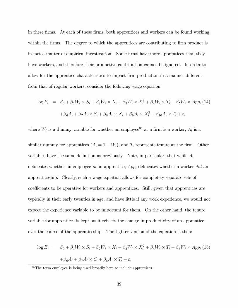
in these firms. At each of these firms, both apprentices and workers can be found working

within the firms. The degree to which the apprentices are contributing to firm product is

in fact a matter of empirical investigation. Some firms have more apprentices than they

have workers, and therefore their productive contribution cannot be ignored. In order to

allow for the apprentice characteristics to impact firm production in a manner different

from that of regular workers, consider the following wage equation:

logEi = β0 + β1Wi × Si + β2Wi ×Xi + β3Wi ×X2i + β4Wi × Ti + β5Wi ×Appi (14)

+β6Ai + β7Ai × Si + β8Ai ×Xi + β9Ai ×X2i + β10Ai × Ti + εi

where Wi is a dummy variable for whether an employee35 at a firm is a worker, Ai is a

similar dummy for apprentices (Ai = 1−Wi), and Ti represents tenure at the firm. Other

variables have the same definition as previously. Note, in particular, that while Ai

delineates whether an employee is an apprentice, Appi delineates whether a worker did an

apprenticeship. Clearly, such a wage equation allows for completely separate sets of

coefficients to be operative for workers and apprentices. Still, given that apprentices are

typically in their early twenties in age, and have little if any work experience, we would not

expect the experience variable to be important for them. On the other hand, the tenure

variable for apprentices is kept, as it reflects the change in productivity of an apprentice

over the course of the apprenticeship. The tighter version of the equation is then:

logEi = β0 + β1Wi × Si + β2Wi ×Xi + β3Wi ×X2i + β4Wi × Ti + β5Wi ×Appi (15)

+β6Ai + β7Ai × Si + β8Ai × Ti + εi

35The term employee is being used broadly here to include apprentices.

39

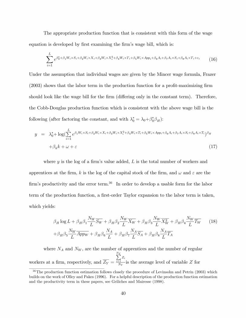
The appropriate production function that is consistent with this form of the wage

equation is developed by first examining the firm’s wage bill, which is:

LXi=1

eβ∗0+β1Wi×Si+β2Wi×Xi+β3Wi×X2

i+β4Wi×T i+β5Wi×Appi+β6Ai+β7Ai×Si+β8Ai×T i+εi (16)

Under the assumption that individual wages are given by the Mincer wage formula, Frazer

(2003) shows that the labor term in the production function for a profit-maximizing firm

should look like the wage bill for the firm (differing only in the constant term). Therefore,

the Cobb-Douglas production function which is consistent with the above wage bill is the

following (after factoring the constant, and with λ∗0 = λ0+β∗0βH):

y = λ∗0+ log(LPi=1

eβ1Wi×Si+β2Wi×Xi+β3Wi×X2i +β4Wi×Ti+β5Wi×Appi+β6Ai+β7Ai×Si+β8Ai×Ti)βH

+βkk + ω + ε (17)

where y is the log of a firm’s value added, L is the total number of workers and

apprentices at the firm, k is the log of the capital stock of the firm, and ω and ε are the

firm’s productivity and the error term.36 In order to develop a usable form for the labor

term of the production function, a first-order Taylor expansion to the labor term is taken,

which yields:

βH logL+ βHβ1NW

LSW + βHβ2

NW

LXW + βHβ3

NW

LX2

W + βHβ4NW

LTW (18)

+βHβ5NW

LAppW + βHβ6

NA

L+ βHβ7

NA

LSA + βHβ8

NA

LTA

where NA and NW , are the number of apprentices and the number of regular

workers at a firm, respectively, and ZY =

NYPi=1

Zi

NYis the average level of variable Z for

36The production function estimation follows closely the procedure of Levinsohn and Petrin (2003) whichbuilds on the work of Olley and Pakes (1996). For a helpful description of the production function estimationand the productivity term in these papers, see Griliches and Mairesse (1998).

40

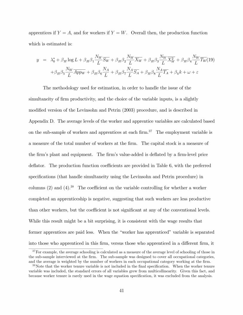
apprentices if Y = A, and for workers if Y =W . Overall then, the production function

which is estimated is:

y = λ∗0 + βH logL+ βHβ1NW

LSW + βHβ2

NW

LXW + βHβ3

NW

LX2

W + βHβ4NW

LTW(19)

+βHβ5NW

LAppW + βHβ6

NA

L+ βHβ7

NA

LSA + βHβ8

NA

LTA + βkk + ω + ε

The methodology used for estimation, in order to handle the issue of the

simultaneity of firm productivity, and the choice of the variable inputs, is a slightly

modified version of the Levinsohn and Petrin (2003) procedure, and is described in

Appendix D. The average levels of the worker and apprentice variables are calculated based

on the sub-sample of workers and apprentices at each firm.37 The employment variable is

a measure of the total number of workers at the firm. The capital stock is a measure of

the firm’s plant and equipment. The firm’s value-added is deflated by a firm-level price

deflator. The production function coefficients are provided in Table 6, with the preferred

specifications (that handle simultaneity using the Levinsohn and Petrin procedure) in

columns (2) and (4).38 The coefficient on the variable controlling for whether a worker

completed an apprenticeship is negative, suggesting that such workers are less productive

than other workers, but the coefficient is not significant at any of the conventional levels.

While this result might be a bit surprising, it is consistent with the wage results that

former apprentices are paid less. When the “worker has apprenticed” variable is separated

into those who apprenticed in this firm, versus those who apprenticed in a different firm, it

37For example, the average schooling is calculated as a measure of the average level of schooling of those inthe sub-sample interviewed at the firm. The sub-sample was designed to cover all occupational categories,and the average is weighted by the number of workers in each occupational category working at the firm.38Note that the worker tenure variable is not included in the final specification. When the worker tenure

variable was included, the standard errors of all variables grew from multicollinearity. Given this fact, andbecause worker tenure is rarely used in the wage equation specification, it was excluded from the analysis.

41

is found that workers who apprenticed in this firm are no different in productivity from

other workers. However, those who apprenticed in another firm are significantly less

productive than those who apprenticed in this firm. This is consistent with the predictions

of the model; the specific human capital acquired in apprenticeship is not transferable to a

new firm. The firm’s ability to extract a surplus from those workers that it has

apprenticed is consistent with the desire of employers to hire their former apprentices.

The other variables are generally of the expected sign. More educated workers are

more productive. Similarly, the sign on the apprentice education variable is positive, but

not significant. The sign on the fraction of apprentices indicates that apprentices may be

less productive than workers, but not significantly so. The coefficient on the tenure of the

apprentices is negative, but not significant. While the negative sign of this coefficient

might be surprising, there are ways in which this is consistent with the apprenticeship

institution. In the initial period of the apprenticeship, the apprentice is often doing odd

jobs, and is very eager to be obedient in order to gain favour with the master.39 During

this period, the apprentice may be as productive as an average unskilled worker in the

enterprise.40 Later in the apprenticeship, when the apprentice is using the firm’s materials

to learn the craft, and occupying more of the master’s time in actual training, the

39Daniel Bas (1989, p. 487) describes this situation in West Africa. “The general view, particularly inWest Africa, is that it [apprenticeship] tends to be too long, and responsibility for this is usually laid atthe door of the master craftsmen who are reluctant to carry out systematic intensive training and therebydeprive themselves too soon of cheap labour or create potential competition. The traditional cultural modelsalso include a long period of ‘socialisation’ during which the apprentice learns to win the acceptance of themaster craftsman and his family by demonstrating his respect and loyalty, thereby progressively meriting theright to learn.” As Ullrich Boehm describes it, “Apprenticeship usually starts with simple labour includingcleaning, washing, fetching water or subsistence agriculture. 62 per cent of the masters ask their apprenticesfor this kind of service beside the work in their trade. Later the apprentice starts learning to know thedifferent tools and work processes of the trade.”40Bas (1989) continues, “During the [initial] socialisation stage the apprentice works as a messenger boy,

doing odd jobs sometimes having no connection with the trade, such as running errands.” This messengerboy activity is more productive for the firm than the period of active training of the apprentice.

42

contribution of the apprentice actually decreases. Still, this variable is not significant.

The reason then why individuals do apprenticeships is for the potential returns that

can accrue to apprenticed workers that become self-employed (specifically, an increased

wage of roughly 19%).41 On the other hand, why do the employers train apprentices?

Our model suggests that the firm’s monopsony power over its former apprentices motivates

such training. A further related reason, as suggested in the other economics article on

apprenticeships in Africa, is that apprenticeship fees can be a significant form of finance for

some firms (Velenchik, 1995). The evidence regarding how much less productive

apprentices are in comparison to other workers is not clear, with the coefficient of interest

not significant in the preferred regression. This fact, coupled with the fact that

apprentices are paid significantly less than other workers, suggests that while the

productive returns of apprentices are less than other workers, they appear to be on net

positive for the firm, although the evidence is weak. Given the errors of the estimates, and

the various costs and benefits of apprenticeship, as outlined earlier, the net benefit for the

firm cannot definitely be signed.

However, another question posed to the firms is of interest on this fact. Firm owners

who trained apprentices were asked if they had ever refused an apprentice. Fifty-eight

percent responded affirmatively. In other words, forty-two percent of those firms that

trained apprentices had never refused an apprentice applicant. Naturally, there is some

endogeneity in the answer, in that potential applicants may not apply for apprenticeship

positions that they know they will not get. Moreover, there may be some selection issues

involved in that the queues may be longer at places that offer ‘better’ apprenticeships.

41A more careful analysis of the net present discounted value of apprenticeship is provided in Appendix E.

43

Still, these responses are concordant with the model where firms are able to set the

apprenticeship fees at a level that makes them at worst indifferent to apprenticeships.

Finally, it is worth returning to the question of whether firms are able to enforce the

optimal long-term wage contract, through reputation effects or other means. As outlined

in the model section, an alternative model is that where long-term contracts are fully

enforceable, and is provided in Appendix C. In this alternative model, those who have

apprenticed within the current firm are more productive and paid more than apprentices

from other firms. The empirical result that apprentices from the current firm are not paid

more than apprentices from other firms is not consistent with this model. Therefore, the

paper also provides some evidence against full contract enforceability in the Ghanaian

context (by reputation or other means), and therefore supports the analysis of Fafchamps

(2004) that enforcing contracts is difficult in the African environment. Moreover, this

paper provides a very concrete example where such difficulty can matter.

In summary, the results are consistent with the model of apprenticeship as training

in specific human capital. Apprenticed workers remaining within the firm are more

productive than apprenticed workers from other firms. However, because their outside

option is no better than apprenticed workers from elsewhere, their wages are not higher

than apprenticed workers from other firms. For this reason, the returns to apprenticeship

are in self-employment, where a former apprentice basically replicates both the technology

and business practice of the apprenticeship firm. Indeed, apprentices are very eager to

enter self-employment, and are constrained only by capital from becoming apprenticed

entrepreneurs.

44

6 Appendix A

Proof of Proposition 1:

The equilibrium concept in use is that of a subgame perfect Nash equilibrium. To

prove the equilibrium, what remains is to show the optimality of the decisions at each step.

That the optimal choice of wage for former apprentices is WF = n in the first order

condition for equation (5) is fairly obvious, but for completeness, consider the Lagrangian

of the optimization problem of the firm’s optimal choice of WF :

L =

Z 1

ρ̂

(c− t+ (1− ρ)(1− λ)(m−WF ))dF (ρ) + δ(WF − n) (20)

First, note that∂WF

∂WF= 1 everywhere and so the constraint qualification clearly holds.

Note also that ∂L∂WF

= 0, since WF > 0. Therefore,

∂L∂WF

= (1− λ)R 1ρ̂(1− ρ)(−1)dF (ρ) + δ = 0. This gives that −(1− λ)[ρ− ρ2

2]1bρ + δ = 0,

since ρ ∼ U(0, 1). So, δ = (1− λ)(12− bρ+ bρ2

2) > 0. Therefore, the constraint binds and

W ∗F = n. The optimality of the wage decisions for outside firms, as well as the quit and

self-employment decisions of workers has already been outlined in the text.

What remains is to show that the firm’s choice of apprenticeship fee is consistent

with optimizing behavior. There are two cases to consider. In the first case, free entry

into providing apprenticeships is allowed. In the second, opposite case, there are

restrictions against entry into providing apprenticeships, and so the firm has monopoly

power for setting the apprenticeship fee.

First, consider the firm’s profit function:

Π =

Z 1

cm−n

(c− t+ (1− ρ) (1− λ) (m− n))dF (ρ) (21)

45

Since ρ ∼ U(0, 1) (by assumption), as noted in the text, the profit function can be

simplified to:

Π = − 1 + λ

2(m− n)c2 +

λ(m− n) + t

(m− n)c− t+

(1− λ)(m− n)

2(22)

for c ≥ 0, and:

Π = c− t+1

2(1− λ)(m− n) (23)

for c ≤ 0 (as the lower bound of the integral cannot fall below 0). Since both pieces (22)

and (23) of the Π function have the same value at c = 0, the profit function Π is

continuous, and is a quadratic for c > 0, and is linear for c < 0. For c > 0, the function is

strictly concave in c, as Π00(c) = −(1+λ)(m−n) < 0, since λ ≥ 0, and m > n (assuming that

apprenticeships are at least marginally productive). For c < 0, Π0(c) = 1 > 0, and Π is

linear. Overall then, the piecewise-defined function (22) and (23) is globally concave (but

not strictly concave), and so it is maximized when the first-order condition, Π0 (c) = 0, i.e.

−(1 + λ)c+ λ(m− n) + t = 0. Therefore, the Π function has a single maximum in the first

quadrant, where c > 0.

Consider then the first case, that of a profit-maximizing monopolist. The unique

choice of apprenticeship fee is:

c∗monop =t+ λ(m− n)

1 + λ(24)

Since the function is globally concave, the second-order conditions are satisfied, and

this is a unique maximum. Recall that in this equilibrium, ρ̂ = cm−n . To confirm that this

is a valid probability (0 < ρ̂ < 1), note that c∗

m−n =t+λ(m−n)(1+λ)(m−n) > 0 always and

t+λ(m−n)(1+λ)(m−n) < 1 ⇐⇒ t < m− n, which is assumed true (that the cost of training to the firm

46

is less than the increase in productivity resulting from the training). Note that, since

m > n, that c > 0, and the apprentice pays the fee to the firm. The profit in the

profit-maximizing case is Πmonop =(m−n−t)2

2(m−n)(1+λ) .

Now, consider the second case, where there is free-entry, resulting in zero profits.

The profit function defined by pieces (22) and (23) has two roots, specifically

c = m− n, t− (1−λ)(m−n)2

. Firms have no incentive to set the apprenticeship fee to the level

of the larger root, m− n. Here, profits are zero because no individual has an incentive to

apprentice as the apprenticeship fee is as large as the (uncertain) returns to apprenticeship.

At the larger root, firms have an incentive to reduce the apprenticeship fee and increase

profits (moving up the right arm of the quadratic). However, the lower root represents a

stable equilibrium. Here, if the firm reduces the apprenticeship fee, it will earn negative

profits. However, it can’t raise the apprenticeship fee without losing all of its apprentices

to competing firms. Therefore, the unique choice of apprenticeship fee for the free-entry

equilibrium is:

c∗FE = t− (1− λ)(m− n)

2(25)

First note that c∗FE may be positive or negative, depending on parameter values. While

the fact that c∗FE < c∗monop is clear from the sketching of the profit function, it can also be

shown algebraically, using the fact that t < m− n, and showing algebraically that

c∗FE < c∗monop is equivalent to t <1+2λ−λ2

2λ(m− n). Since 1 + 2λ− λ2 > 2λ, as 0 < λ < 1,

this result will always hold.

47

7 Appendix B

In this appendix, we consider the case where the firm takes into account the competitive

implications of providing apprenticeships. That is, in this model, providing

apprenticeships has the potential to increase the firm’s competition, specifically from those

former apprentices who become self-employed. This is handled in the model by including

this competitive cost in the firm’s profit function. It should be noted that such a cost is

not already included in the firm’s cost of training the apprentices, t. The training cost t

applies to all apprentices, while the competitive cost to the firm of training apprentices will

apply only to those former apprentices that become self-employed. Therefore, this case

needs to be handled separately. The firm’s new profit function then is:

Π =

Z 1

ρ̂

(c− t+ (1− ρ) (1− λ) (m−WF )− ρq)dF (ρ) (26)

subject to the constraints that ρ̂ ≥ 0, and ρ̂ ≤ 1, and WF ≥ n. As in the model

outlined in the main paper and Appendix A, firms will again choose WF = n, and for

apprenticeship, the equilibrium cut-off for ρ will be ρ̂ = cm−n . Therefore c ≥ 0, and

c ≤ m− n. The competitive cost, ρq, for each apprentice, is a function of that apprentice’s

probability of becoming self-employed. Workers with low probability of becoming

self-employed impose little competitive cost, a priori, on the firm. This profit function

simplifies to the following, again under the uniform density assumption, as before:

Π = c2[q − (1 + λ)(m− n)

2(m− n)2] + c[

t+ λ(m− n)

m− n] +

1

2(1− λ)(m− n)− q

2− t (27)

In this case the first-order condition for an interior solution is:

c[q − (1 + λ)(m− n)

(m− n)2] +

t+ λ(m− n)

m− n= 0 (28)

48

This simplifies to:

c =λ(m− n) + t

1 + λ− qm−n

(29)

Therefore, the solution is similar to the previous profit-maximizing solution, with

the additional consideration of the competitive cost in the term, qm−n . As this competitive

cost, q, increases, the cost charged by firms will increase, in order to reduce the number of

apprentices that they train, and reduce the negative competitive impact. Mathematically,

this follows from the following: ∂c∂q= (m−n)[λ(m−n)+t]

[(1+λ)(m−n)−q]2 > 0. Consider the second-order

condition for the profit function: ∂2Π∂c2

= q−(1+λ)(m−n)(m−n)2 . Consider the extreme case of this

second-order condition first. If q ≥ (1 + λ)(m− n), then the profit function is everywhere

convex. The only extremum is a minimum, and it occurs when c < 0. Therefore, since the

second-derivative is positive, profit will be maximized at the upper-bound for c, namely,

c = m− n. Here, ρ̂ = 1, and no one apprentices. Therefore, the maximum profit is also a

zero-profit equilibrium, and it involves no apprenticeship. This equilibrium will only occur

if the competitive cost is sufficiently high, specifically, if the competitive cost, q, per worker

that gains self-employment is significantly larger than the productivity boost from

apprenticeship, m− n. If this competitive cost is sufficiently high, then firms would be

forced to charge an apprenticeship fee that is prohibitive for potential apprentices.

On the other hand, if q < (1 + λ)(m− n), then ∂2Π∂c2

< 0, and the profit function is

strictly concave. There are two cases to consider on this region. If q ≥ m− n− t (and

q < (1 + λ)(m− n)), then the constraint c = m− n will bind for profit maximization.

That is to say that the best that firms can do is to make zero profits by inducing no

apprenticeship, as in the case above where q ≥ (1+λ)(m−n). Here, while the competitive

cost q is not as large as before, it is larger than the productive benefit of apprenticeship

49

(m− n), less the costs of training (t), and so apprenticeship does not make economic sense.

On the other hand, if q < m−n− t, then the optimal choice of apprenticeship fee will occur

at an interior solution defined by c in equation (29). Here, the second-order condition is

also satisfied. Firm profits will be: Π = (m−n−t−q)22[(1+λ)(m−n)−q] . What is clear from the profit

function is that the base model of Appendix A is a special case of this model when q = 0.

We can also consider the case of the competitive equilibrium, where free entry

results in zero profits for the firm. Consider the two cases. In the first case, if

q ≥ (1 + λ)(m− n), the profit function is convex, and as already noted, the zero profit

equilibrium that will be chosen is also the profit maximizing equilibrium, where c = m− n,

and no one apprentices. Consider the more interesting case of the concave profit function

where q < (1 + λ)(m− n). Therefore, for profits to be zero, consider the two roots of the

above equation (27): c = 2t−(1−λ)(m−n)+q1+λ− q

m−n, c = m− n. In the case where q ≥ m− n− t,

c = m− n is the lower of the two roots, but is also an upper bound on c. As noted above,

this profit-maximizing case will also be the zero-profit equilibrium for

m− n− t < q ≤ (1 + λ)(m− n). Now, consider the more interesting case where

q < m− n− t. This is the case where the competitive cost per worker that becomes

self-employed is less than the productive increase in apprenticeship (m− n) less the

training cost (t). In this case, the lower root will be c = 2t−(1−λ)(m−n)+q1+λ− q

m−n, provided that bρ

remains positive. This will occur if q ≥ (1− λ)(m− n)− 2t. Again, the upper root

c = m− n will not be an equilibrium. Rather, as in the case in Appendix A, firms will

compete with each other on the apprenticeship fee, lowering it until it reaches

c = 2t−(1−λ)(m−n)+q1+λ− q

m−n, the other zero profit equilibrium. Now, consider the case where the

bρ = 0 constraint binds, which will occur when q < (1− λ)(m− n)− 2t. Here, firm profits

50

are Π = c− t− q2+ 1

2(1− λ)(m− n). Therefore, the zero-profit solution on this region has

c = t+ q2− 1

2(1− λ)(m− n).

Therefore, to summarize, the profit-maximizing and zero profit equilibrium is the

same for q ≥ m− n− t . In this case, the equilibrium apprenticeship fee is given by

c = m− n, and profits are zero in this case, as no one apprentices. If q < m− n− t, then

for the profit-maximizing equilibrium, the apprenticeship fee is given by c = λ(m−n)+t1+λ− q

m−n, with

bρ = λ(m−n)+t(1+λ)(m−n)−q , and Π = (m−n−t−q)2

2[(1+λ)(m−n)−q] . For the zero-profit equilibrium on

q < m− n− t, there are two cases. For (1− λ)(m− n)− 2t ≤ q < m− n− t, the

apprenticeship fee is given by c = 2t−(1−λ)(m−n)+q1+λ− q

m−n, and bρ = 2t+q−(1−λ)(m−n)

(1+λ)(m−n)−q . For

q < (1− λ)(m− n)− 2t, the apprenticeship fee is given by c = t+ q2− 1

2(1− λ)(m− n), and

bρ = 0. In any case, the main predictions remain as before when apprenticeship occurs.Since WF = n, those who have apprenticed within the current firm are more productive

than apprentices from elsewhere, but need not be paid more than other apprentices, and

therefore, the returns to apprenticeship continue to lie in self-employment.

51

8 Appendix C

In this appendix, we abstract from the problems of time-inconsistency in the firm’s wage

offer. If we abstract from these problems, then it could be possible for the firm to commit,

ahead of time, to a wage that is higher than the worker’s outside offer. More specifically,

suppose that the firm is able to write a binding (and enforceable, in the Ghanaian context)

contract at the time of the apprenticeship agreement that commits itself to a particular

wage for the apprenticed worker should that worker remain in the firm upon completion of

the apprenticeship. While the binding nature of such a contract is probably not realistic

for the Ghanaian situation (see Fafchamps (2004) and the discussion in the paper), we can

compare this equilibrium where full contracting is allowed to the more realistic case of

Appendix A in terms of predictions, and implications for firm profits. These theoretical

predictions can be examined on their own terms, and can also be empirically tested in the

data, to see whether one model is preferred. In the case of this appendix, where the within

firm wage contract is enforceable ex ante, the analysis follows exactly as in the main paper

up to (4):

Maxc,WF

Π =

Z 1

ρ̂(c,WF )

(c− t+ (1− ρ)(1− λ)(m−WF ))dF (ρ) (30)

The firm will maximize profits subject to the three constraints: i) WF ≥ n (the

firm can pay no less than the worker’s outside option), ii) ρ̂ ≥ 0, and iii)ρ̂ ≤ 1. Two

further constraints will be added below, namely that iv) WF ≤ m, and v) c ≤ m− n. This

is to say that the firm cannot commit in the aforementioned contract to pay its apprenticed

workers more than their productive contribution to output (WF ≤ m), and the firm cannot

charge an apprenticeship fee that is larger than the increase in productivity resulting from

52

the apprenticeship (c ≤ m− n). Note also that in the case described in this appendix, the

firm can jointly decide (and commit to) both the apprenticeship fee, c, and the wage

offered to its former apprentices within the firm, WF . Constraint ii) can be written more

explicitly. Note that if we substitute WO = n and Wn = n into equation (2), and simplify,

we will get the result that:

ρ̂ =c+ (1− λ)(n−WF )

m− λn− (1− λ)WF(31)

Since the denominator in this is always strictly positive anywhere, as a result of constraint

iv), we can see that constraint ii) can be rewritten as c+ (1− λ)(n−WF ) ≥ 0.

Furthermore, given the other constraints, constraint v) can be shown to be equivalent to

constraint iii), and is therefore dropped, and so constraint iii) can be shown to be written

as: m− n− c ≥ 0. Now, the Lagrangian for the firm’s profit-maximization problem is:

L =

Z 1

ρ̂(c,WF )

(c− t+ (1− ρ)(1− λ)(m−WF ))dF (ρ) (32)

+α1(WF − n) + α2(n+c

1− λ−WF ) + α3(m− n− c) + α4(m−WF )

where ρ̂(c,WF ) is as given in equation (31). I will consider separately the cases of

an interior solution, and the boundary solution to find the profit maximization point(s).

First, find the critical points of the profit function, by setting ∂Π∂c= 0 and ∂Π

∂WF= 0. First,

for ∂Π∂c= 0, noting from equation (31) that ∂ρ̂

∂c= 1

m−λn−(1−λ)WF:

Z 1

c+(1−λ)(n−WF )

m−λn−(1−λ)WF

(1)dρ (33)

− 1

m− λn− (1− λ)WF[c− t+ (1− c+ (1− λ)(n−WF )

m− λn− (1− λ)WF)(1− λ)(m−WF )] = 0

53

Some algebraic work will show that this will give an explicit expression for c:

c =(1− λ)tWF − λ(m− n)2 − tm+ λtn

(1− λ)WF − (1 + λ)m+ 2λn(34)

Now, consider the first-order condition with respect to WF . First note that, from

equation (31) and some algebraic manipuluation, we can get that ∂ρ̂∂WF

= (1−λ)(n−m+c)(m−λn−(1−λ)WF )2

.

Therefore for ∂Π∂WF

= 0, we get:

−Z 1

c+(1−λ)(n−WF )

m−λn−(1−λ)WF

(1− λ)(1− ρ)dρ (35)

− (1− λ)(n−m+ c)

(m− λn− (1− λ)WF )2[(c− t) + (1− λ)(m−WF )(1−

c+ (1− λ)(n−WF )

m− λn− (1− λ)WF)] = 0

This will simplify to an implicit expression for WF :

(1− λ)WF (m− n− 2t) + (1− λ)cWF (36)

+( 3λn− (1 + 2λ)m)c+ (2λ− 1)m2 + (1− 3λ)mn+ λn2 + 2tm− 2λtn = 0

Therefore, the solution to equation (36) and equation (34) will yield the set of all

critical points for the profit function. Substituting the expression for c from equation (34)

into equation (36) gives:

(1− λ)WF (m− n− 2t) + (1− λ)((1− λ)tWF − λ(m− n)2 − tm+ λtn

(1− λ)WF − (1 + λ)m+ 2λn)WF (37)

+( 3λn− (1 + 2λ)m)((1− λ)tWF − λ(m− n)2 − tm+ λtn

(1− λ)WF − (1 + λ)m+ 2λn) +

( 2λ− 1)m2 + (1− 3λ)mn+ λn2 + 2tm− 2λtn = 0

After considerable manipulation, this equation in WF simplifies to:

(1−λ)2(m−n− t)W 2F − 2(1−λ)(m−n− t)(m−λn)WF +(m−n− t)(m−λn)2 = 0 (38)

54

This quadratic equation has a unique solution (the discriminant is 0):

WF =m− λn

1− λ(39)

Substituting this expression for WF back into equation (34) yields:

c = m− n (40)

However, this is merely constraint iii). Moreover, since m > n, we can show from

equation (39) that WF > m, which violates constraint iv). Therefore, the unique critical

point for the profit function lies outside of our constrained set. Therefore, in order to

determine the profit-maximizing solution, we need only consider the boundary cases, which

we will now do.

We can consider the cases where any combination of the following four constraints

bind: i) WF ≥ n, ii) c+ (1− λ)(n−WF ) ≥ 0, iii)c ≤ m− n, iv)WF ≤ m. Clearly, i)

and iv) will not bind at the same time. Suppose that i) binds (WF = n). Then, ρ̂ = cm−n .

In this case, firm profits reduce to:

Π = 12(m−n) [−c2(1− λ) + 2c(λ(m− n) + t)− 2(m− n)t+ (1− λ)(m− n)2]. The optimal

choice of c in this case can be shown (using first and second-order conditions) to be:

c = λ(m−n)+t1−λ . So, this is exactly the case outlined in the main paper (and Appendix A),

where the firm is forced to keep wage offers time-consistent. Clearly, none of the other

constraints will bind then, when constraint i) binds. In this case, firm profits are:

Πi =(m−n−t)2

2(m−n)(1+λ) .

Now, suppose that constraint iv) binds, (WF = m). In this case, ρ̂ = c−(1−λ)(m−n)λ(m−n) ,

and the firm profit function reduces to: Πiv =(c−t)(m−n−c)

λ(m−n) . Here, it can be shown,

55

through first and second-order conditions, that the profit-maximizing choice of

apprenticeship fee is c = m−n+t2, and that in this case firm profits are: Πiv =

(m−n−t)24λ(m−n) (*).

Next, suppose that constraint ii) binds (c = (1− λ)(WF − n)). In this case, ρ̂ = 0,

and Π = 12(1− λ)(m+WF − 2n)− t. Since ∂Π

∂WF= 1

2(1− λ) > 0, to maximize profits when

constraint ii) binds, the firm would increase WF until constraint iv) binds, so that

WF = m. However, substituting the two binding constraints, we get that firm profits are:

Πii,iv = (1− λ)(m− n)− t. This is obviously not the same solution as the maximum profit

when iv) binds alone. Therefore, we expect that firm profits here should be less than the

optimal case where iv) binds above (*). That is we would like to show that Πiv > Πii,iv.

This amounts to showing that (m−n−t)2

4λ(m−n) > (1− λ)(m− n)− t. But this inequality is

equivalent to [(2λ− 1)(m− n)− t]2 > 0, which is always true. Therefore Πiv > Πii,iv.

Next, suppose that constraint iii) binds (c = m− n). First, consider the

apprenticeship decision in this case. The expected returns to apprenticeship are:

−(m− n) + ρm+ (1− ρ)[λn+ (1− λ)WF ], while the returns from not apprenticing are n.

Therefore, to induce apprenticeship we need that the returns from apprenticeship are at

least as large as n. This can be shown to be equivalent to WF ≥ m−λn1−λ . But, again since

m−λn1−λ > m, this lies outside our constraint set (and the equality version of this is just the

critical point that we ruled out earlier). Therefore, constraint iii) does not bind at the

optimal solution.

So, the cases that have not yet been ruled out are when constraint i) binds, and

when constraint iv) binds. To show the profits on the region where constraint i) binds are

never larger than the profits when constraint iv) binds, consider the following. For

Πi > Πiv,(m−n−t)2

2(m−n)(1+λ) >(m−n−t)24λ(m−n) . But, this can be shown to be equivalent to λ > 1.

56

However, by the definition of λ as a proportion, 0 < λ < 1. Therefore, Πi < Πiv, and so

the profit maximizing solution occurs when constraint iv) binds, that is when, WF = m,

c = m−n+t2, ρ̂ = c−(1−λ)(m−n)

λ(m−n) , and Πiv =(m−n−t)24λ(m−n) . So, in this case, firms do pay their

former apprentices their marginal products in terms of a wage. Firms still make more

profits here than in the case of constraint i) binding (Appendix A), as they charge a very

high apprenticeship fee, civ = m−n+t2

> t+λ(m−n)1+λ

= cmonop in Appendix A. The difference in

profits between this case and the case of Appendix A

( (m−n−t)2

4λ(m−n) −(m−n−t)2

2(m−n)(1+λ) =(1−λ)(m−n−t)24λ(1+λ)(m−n)2 > 0) can be seen as the foregone profits that firms

lose as a result of being unable to engage in binding contracts.

Case of Free Entry:

We can also consider the equilibrium that would result when there is free entry into

the provision of apprenticeships. As in the main case in the text, here the result will be

driven by a zero-profit condition. This case can be solved by setting equation (30) above

equal to zero subject to the same constraints as in the previous section, namely: i) WF ≥ n,

ii) ρ̂ ≥ 0, iii)ρ̂ ≤ 1, iv) WF ≤ m, and v) c ≤ m− n. It can be shown that in this context,

neither constraint iii) nor v) will bind. Provided that ρ̂ > 0, equation (30) will give:

[(c− t)ρ+ (1− λ)(m−WF )(ρ−1

2ρ2)]1c+(1−λ)(n−WF )

m−λn−(1−λ)WF

= 0

This will result in the following condition, after some simplification:

(m− n− c)[2(c− t)(m− λn− (1− λ)WF ) + (1− λ)(m−WF )(m− n− c)] = 0 (41)

The first case where profits will be zero is the case c = m− n. This case was

outlined above for constraint iii) binding, and the wage required to induce apprenticeship

57

lies outside our constraints in this case. The case that remains where profits will be zero

occurs when the second factor is 0, that is when:

2(c− t)(m− λn− (1− λ)WF ) + (1− λ)(m−WF )(m− n− c) = 0 (42)

This equation is a function of the two choice variables for the firm, c, and WF . It

defines a hyperbola in the (c,WF ) space. Using extensive functional analysis42 and ruling

out the inconsistent cases, the single segment of the hyperbola that defines the solution set

within the constraints is a concave, upward-sloping curve between points

A(2t−(1−λ)(m−n)1+λ

, n) and B(t,m). This is the solution provided that ρ̂ > 0 always, which

can be shown to be true if (1− λ)(m− n) ≤ t. Now, consider when constraint ii) binds,

that is when ρ̂ = 0. It can be shown that this will occur for a non-trivial set provided that

(1− λ)(m− n) > t. In this case, the zero-profit solutions consist of the hyperbola defined

by equation (42) between points A(2t−(1−λ)(m−n)1+λ

, n) and

C(2t− (1− λ)(m− n), 2t1−λ + 2n−m) combined with the contiguous line CB, with B

defined above.43 Therefore, in either case ((1− λ)(m− n) ≤ t or (1− λ)(m− n) > t), the

zero-profit solution will consist of an upward-sloping continuous curve joining points A and

B, defined above. Note that point A corresponds to the solution from the time-consistent

equilibrium outlined in the main paper and Appendix A. Since n > 0 and m > 0, we know

that this curve from A to B lies within the first two quadrants of the (c,WF ) space

(thankfully—otherwise workers would be paying firms to work). However, 2t−(1−λ)(m−n)1+λ

can

be positive or negative depending on parameters. That is, in some cases c < 0 , and the

42

The full details are available from the author upon request, but this work is too tedious to take up spacehere.43The equation of this line is given by setting bρ = 0 in equation (30).

58

firm will pay the apprentices in order to apprentice within the firm. The upper bound on c

is the cost of training, t, and n ≤WF ≤ m on this segment. It should also be noted that

∂c∂WF

> 0, that is if the wage WF is raised, then the apprenticeship fee must also be raised

to maintain zero profits.

In summary, the case of free entry allows for a continuum of equilibria, with wages

ranging anywhere within their bounds, from n to m. Therefore, the free-entry equilibria

with full contracting commitments will all but surely be consistent with the data.

Consider the more interesting case of profit-maximizing firms. Here, firms will pay their

former apprentices their marginal product, m, in equilibrium. Therefore, this model

predicts that workers who have apprenticed within the current firm should be both more

productive than apprentices from elsewhere, and paid more than apprentices from

elsewhere. The latter point differs from the main model of Appendix A, and therefore

these different predictions can be compared in the data.

59

9 Appendix D - Production Function Estimation

For simplicity, we will rewrite the production function in equation (19) as follows:

yft = β∗∗0 + (XV )ft(βV ) + βkkft + ωft + εft (43)

where β∗∗0 = λ0 + β∗0βH , XV is the row vector containing {logL, SW , XW , X2W , TW ,

AppW , NA

L, SA, TA}, and βV is the column vector containing βH , βHβ1, βHβ2, βHβ3, βHβ4,

βHβ5, βHβ6, βHβ7, βHβ8}. In basic least squares production function estimation, the

residual in the estimation consists of both the firm productivity, ω, as well as the

conventional noise component, ε. The basic idea (although far more formally elaborated)

of both Olley and Pakes (1996) and Levinsohn and Petrin (2003) is to try to control more

carefully for firm productivity, as it could well be correlated with the inputs, particularly

the labor inputs, XV , which would result in biased parameter estimates. Olley and Pakes

develop a proxy measure for productivity based on a firm’s use of investment, and

Levinsohn and Petrin develop a proxy based on the firm’s use of intermediate inputs. It is

the Levinsohn and Petrin procedure followed here. Levinsohn and Petrin consider the

following intermediate input demand function:

mft = ft (ωft, kft) (44)

In order to write the function in this way, input prices are assumed to be common across

firms within a given time period, and so the intermediate input function is indexed by t.

In order for intermediate inputs to be a valid proxy for productivity, the intermediate input

use must be monotonically increasing in ω, as in the case of investment. Levinsohn and

Petrin provide the conditions under which this is the case. Then, equation (44) can be

60

inverted to get:

ωft = f−1t (mft, kft) (45)

We can then substitute this expression into equation (43) to get:

yft = β∗∗0 + (XV )ft(βV ) + βkkft + f−1t (mft, kft) + εft (46)

The f−1t is allowed to be a nonparametric function of m and k. As a result, initially,

the βk coefficient cannot be separately identified from the nonparametric function.

Therefore, define this combined function as φt(mft, kft) = βkkft + f−1t (mft, kft). Then,

equation (46) can be rewritten as:

yft = β∗∗0 + (XV )ft(βV ) + φt(mft, kft) + εft (47)

The φ function is nonparametric function, and so equation (47) is a partially linear

model, which can be estimated using any semiparametric estimation technique. The

method that I use is that of Robinson (1988), which is also described in Levinsohn and

Petrin (2003). This estimation is labelled as the ‘first stage’ of the Levinsohn and Petrin

estimation procedure, and gives a consistent estimate of the parameters βV . The ‘second

stage’ of the Levinsohn and Petrin procedure involves the identification of the capital

coefficient, and the assumptions of this second stage are given in Levinsohn and Petrin

(2003). While I do estimate the capital coefficient according to this procedure, the capital

coefficient is of no interest for the current study, and so I do not describe the rest of the

procedure here. None of the assumptions (limited as they are) of the second stage

procedure are required for the identification of βV , and so those assumptions are not

described here either.

61

10 Appendix E - Net Benefits of Apprenticeship

This appendix measures the net present discounted value of apprenticeship, according to

the model, and the coefficient estimates of Table 4. It should be noted that these

estimated benefits are very rough calculations, as they are calculated at the averages of the

variables, and using the point estimates. I do not bother to calculate confidence bounds on

these estimates, as once the standard errors on each of the coefficient estimates are taken

into account, the bounds would be very large indeed. That being said, these estimated net

benefits can provide some "back-of-the-envelope" measures of the net benefits of

apprenticeship, and at least ensure that they are positive for those who undertake

apprenticeship.

The net benefits of apprenticeship can be calculated from the terms in equation (2).

In order to calculate the net benefits in the population as a whole, we use the GLSS data,

and the estimated coefficients from Table 4. Here, we do not know whether a former

apprentice is working in the same firm as the firm in which an apprenticeship was

completed or not. Therefore, a more general measure of the ex-ante net expected wages if

a worker completes an apprenticeship is:

NPVapp + ρNPVA−SE + (1− ρ)NPVA−EE (48)

The first term, NPVapp, is the net monetary returns during the apprenticeship, and

will include the apprentice wages minus apprenticeship fees (this was labelled −c in the

simple two period model). While in the model, the value c included both pecuniary and

non-pecuniary transfers between the apprentice and the firm owner, here we will focus on

the pecuniary transfers (i.e. including both cash and in-kind allowances, but abstracting

62

from how ‘hard’ the apprentice works in apprenticeship versus alternative employment, for

example). The variable ρ is the usual probability of obtaining capital to start

self-employment. Here, NPVA−SE is the net present discounted value of the

post-apprenticeship wage returns in self-employment, while NPVA−EE is the net present

discounted value of the post-apprenticeship wage returns in employee wage work. On the

other hand, the ex-ante net expected wages if a worker does not complete an

apprenticeship are:

ρNPVNA−SE + (1− ρ)NPVNA−EE (49)

where the NPVNA−SE is the net present discounted value of the self-employment

wage for non-apprenticed workers, and the NPVNA−EE is the net present discounted value

of the employee wage for non-apprenticed workers. Therefore, the ex-ante returns to

apprenticeship are positive if Net Benefit = (48) - (49) > 0. We will now discuss how

expressions (48) and (49) can be estimated using the data, and the results of the paper.

First, consider the net monetary returns during the apprenticeship period, NPVapp.

Let the discount factor be β and the apprenticeship wages in a single year be Wapp. Also,

we will assume for simplicity that the apprenticeship fees are paid at the beginning of the

apprenticeship period (the data in the GLSS does not distinguish when the apprenticeship

fees are paid). Then, the net monetary return during apprenticeship, using an

apprenticeship period of 3 years, which is the average (technically 2.92) in the data, is

given by:

NPVapp = −fee+Wapp + βWapp + β2Wapp (50)

Now, consider the net present discounted value of the post-apprenticeship earnings

63

in self-employment, NPVA−SE. If a worker ceases to work in T periods from now, then

NPVA−SE will be calculated over the periods from t = 3 until t = T (as the apprentice is

engaging in the apprenticeship in periods t = 0, 1, 2). Therefore, we get:

NPVA−SE =TPt=3

βtWA−SE =β3(1− βT−2)WA−SE

1− β(51)

where WA−SE is the single-year earnings for former apprentices in self-employment.

Similarly, we get that NPVA−EE =β3(1−βT−2)WA−EE

1−β , where WA−EE is the single-year wage

for former apprentices in employee work. On the other hand, workers that do not engage

in an apprenticeship can begin earning their returns immediately, and therefore

NPVNA−SE =TPt=0

βtWNA−SE =(1−βT+1)WNA−SE

1−β , and

NPVNA−EE =TPt=0

βtWNA−EE =(1−βT+1)WNA−EE

1−β , where WNA−SE and WNA−EE are the

single-year earnings to non-apprenticed workers in self-employment and employee work,

respectively.

Since in this exercise we are interested in the ex-ante returns to apprenticeship, each

of the earnings measures, WA−SE , WA−EE, WNA−SE, and WNA−EE, is calculated at the

mean values of all individuals in the Ghanaian labor force, that is using the data in the first

panel of Table 1b, and using the relevant regression coefficients of Table 4 (i.e. column (6)

for the self-employment earnings, and column (9) for the employee earnings, including the

correction terms). The apprenticeship wage, Wapp, is merely taken as the average earnings

among all those who are currently engaged as apprentices in the GLSS survey. The

apprenticeship fee, fee, is taken as the average fee paid by those who are currently engaged

in apprenticeship. The parameters upon which we have discretion are the probability of

receiving capital, ρ, the discount factor, β, and the length of one’s remaining working life at

64

the date of the apprenticeship decision, T . In Ghana, in 1999, the life expectancy at birth

for men was 57 years. Since the life expectancy upon reaching one’s early twenties would

be higher than this, we will arbitrarily set the end of one’s working life at 60 years.44 Since

the average age of apprentices is 23 years old, and the apprenticeship is 3 years in length,

on average people are making the apprenticeship decision at age 21, with 39 years of

working life remaining after the current year (T = 39). For simplicity, we will take ρ = 0.5.

Therefore, initially, we will measure the net benefits of apprenticeship for those who have a

50 percent chance ex-ante of receiving the capital to start their own firm. Higher values of

ρ would naturally increase the net benefit, while lower values would decrease it. For the

discount factor, we will take β to be 0.9 or 0.95 (corresponding to a discount rate of 0.05 or

0.10). For an average labor force member, with ρ = 0.5, the present discounted value of

the net benefit of apprenticeship is 85 000 cedis (for β = 0.90) and 270 000 cedis (for

β = 0.95), that is approximately 2 or 7 months earnings for an average labor force member.

Now, we can also measure the ex-ante net benefit of apprenticeship, using the

characteristics of those who actually take up an apprenticeship. Since the fraction of

current apprenticed workers who become self-employed is 0.658, we can take that value for

ρ, along with the characteristics of the sub-set of the population that takes up

apprenticeship to calculate the ex-ante net benefit for this group. For ex-post apprenticed

workers, then, the ex-ante net benefit of apprenticeship is 110 000 cedis (for β = 0.90) and

350 000 cedis (for β = 0.95 ), or approximately 3 or 8 months earnings, respectively.

Again, given the assumptions and use of averages, etc., these numbers should be taken as

indicating order of magnitude rather than precise predictions, but they do indicate positive

44Retirement is not an issue before this age in Ghana.

65

discounted net present value returns from apprenticeship, for those who apprentice.

.

66

References

Acemoglu, D., 1997. Training and Innovation in an Imperfect Labour Market. Review ofEconomic Studies 64, 445—464.

Acemoglu, D., Pischke, J.S., 1999. The Structure of Wages and Investment in GeneralTraining. Journal of Political Economy 107, 539—572.

Acemoglu, D., Pischke, J.S., 1998. Why do Firms Train? Theory and Evidence. QuarterlyJournal of Economics 113, 79—119.

Appleton, S., Hoddinott, J., Mackinnon, J., 1996. Education and Health in Sub-SaharanAfrica. Journal of International Development 8, 307-339.

Aryeetey, E., Baah-Nuakoh, A., Duggleby, H., Hettige, H., and Steel, W.F., 1994. TheSupply and Demand for Finance among SMEs in Ghana, Discussion Paper 251, AfricaTechnical Department, Washington D.C.: World Bank.

Bas, D., 1989. On-the-job Training in Africa. International Labour Review 128, 485—496.

Beaudry, P., Sowa, N.K., 1994. Ghana, in: Horton, S., R. Kanbur, and D. Mazumdar(Eds.), Labor Markets in an Era of Adjustment, Vol. 2 World Bank, Washington, D.C.

Becker, G. S., 1964. Human Capital: A Theoretical and Empirical Analysis, with SpecialReference to Education. Columbia University Press, New York.

Bennell, P., 1996. Rates of Return to Education: Does the Conventional Pattern Prevail insub-Saharan Africa? World Development 24, 183-199.

Berry, S. 1985. Fathers Work for their Sons. University of California Press, Berkeley, CA.

Birks, S., Fluitman, F., Oudin, X., and Sinclair, C., 1994. Skills Acquisition inMicro-Enterprises: Evidence from West Africa. OECD, Paris.

Boehm, U., 1997. Human Resource Development in African Small- and Micro-Enterprises:The Role of Apprenticeship, in: Bass, H.H. et.al. (Eds.), African Development PerspectivesYearbook 1996 - Regional Perspectives on Labour and Employment. LIT Verlag, Münster.

Boissiere, M., Knight, J.B. and Sabot, R.H. Earnings, Schooling, Ability, and CognitiveSkills. American Economic Review 75, 1016-1030.

Callaway, A. 1964. Nigeria’s Indigenous Education: The Apprentice System. Odu:University of Ife Journal of African Studies 1(1), 62-79.

Davidson, R. and MacKinnon, J. Estimation and Inference in Econometrics. OxfordUniversity Press, New York.

Felli, L. and Harris, C., 1996. Learning, Wage Dynamics and Firm-Specific HumanCapital. Journal of Political Economy 104, 838—868.

67

Frazer, G., 2003. Linking Firms and Workers: Heterogeneous Labor and Returns toEducation, mimeo, University of Toronto.

Glewwe, P., 1999. The Economics of School Quality Investments in Developing Countries:An Empirical Study of Ghana. MacMillan Press, Houndmills, U.K.

Glick, P. and Sahn, D.E. 1997. Gender and Education Impacts on Employment andEarnings in West Africa: Evidence from Guinea. Economic Development and CulturalChange 45, 793-823.

Griliches, Z. and Mairesse, J., 1998. Production Functions: The Search for Identification,in: Strøm, S. (Ed.), Econometrics and Economic Theory in the Twentieth Century: TheRagnar Frisch Centennial Symposium. Cambridge University Press, Cambridge, UK.

Hazlewood, A., Armitage, J., Berry, A., Knight, J., Sabot, R., 1989. Education, Work andPay in East Africa. Clarendon Press, Oxford, U.K.

Heckman, J.J., 1979. Sample Selection Bias as a Specification Error. Econometrica 47,153—161.

Jones, P., 2001. Are Educated Workers Really More Productive? Journal of DevelopmentEconomics 64, 57-79.

Jovanovic, B., and Nyarko, Y., 1995. The Transfer of Human Capital. Journal of EconomicDynamics and Control 19, 1033—1064.

Khandker, S.R., Samad, H.A., and Khan, Z.H., 1998. Income and Employment Effects ofMicro-credit Programmes: Village-level Evidence from Bangladesh. Journal ofDevelopment Studies 35, 96-124.

King, K. 1977. The African Artisan: Education and the Informal Sector in Kenya.Heinemann, London.

Knight, J. and Sabot, R. 1990. Education, Productivity, and Inequality: The East AfricanNatural Experiment. Oxford University Press, New York.

Lall, S. and Pietrobelli, C. 2002. Failing to Compete: Technology Development andTechnology Systems in Africa. Edward Elgar, Cheltenham, UK.

Lall, S., Navaretti, G.B., Teitel, S., and Wignaraja, G., 1994. Technology and EnterpriseDevelopment: Ghana under Structural Adjustment. St. Martin’s Press, New York.

Lee, L.-F., 1978. Unionism and Wage Rates: A Simultaneous Equations Model withQualitative and Limited Dependent Variables. International Economic Review 19, 415—433.

Lee, L.-F., Maddala, G.S., Trost, R.P., 1980. Asymptotic Covariance Matrices ofTwo-Stage Probit and Two-Stage Tobit Methods for Simultaneous Equations Models withSelectivity. Econometrica 48, 491-503.

68

Levinsohn, J., Petrin, A., 2003. Estimating Production Functions Using Inputs to Controlfor Unobservables. Review of Economic Studies 70, 317-341.

Levy, B., 1993. Obstacles to Developing Indigenous Small and Medium Enterprises 7, 65-83.

Mazumdar, D. and Mazaheri, A. 2003. The African Manufacturing Firm. Routledge,London.

McKernan, S-M., 2002. The Impact of Microcredit Programs on Self-Employment Profits:Do Noncredit Program Aspects Matter? Review of Economics and Statistics 84, 93-115.

Morduch, J., 1999. The Microfinance Promise. Journal of Economic Literature 37,1569-1614.

Mwabu, G., Schultz, T.P., 1996. Education Returns Across Quantiles of the WageFunction: Alternative Explanations for Returns to Education by Race in South Africa.American Economic Association Papers and Proceedings, 86, 335-339.

Nissanke, M., Aryeetey, E., 1998. Financial Integration and Development: Liberalizationand Reform in Sub-Saharan Africa. Routledge, London.

Nielsen, H., Westergård-Nielsen, N., 2001. Returns to Schooling in Less DevelopedCountries: New Evidence from Zambia. Economic Development and Cultural Change,January, 364-394.

Olley, S., Pakes, A., 1996. The Dynamics of Productivity in the TelecommunicationsEquipment Industry. Econometrica 64, 1263—97.

Oyeneye, Olatunji Y., 1981. Factors Influencing Entry into the Informal SectorApprenticeship System: The Nigerian Case. African Social Research, December 1981, 1-27

Pagan, A., Vella, F., 1989. Diagnostic Tests for Models Based on Individual Data: ASurvey. Journal of Applied Econometrics 4, S29-S59.

Pitt, M.M., Khandker, S.R., 1998. The Impact of Group-Based Credit Programs on PoorHouseholds in Bangladesh: Does the Gender of Participants Matter? Journal of PoliticalEconomy 106, 958-996.

Prendergast, C., 1993. The Role of Promotion in Inducing Specific Human CapitalAcquisition. Quarterly Journal of Economics 108, 523—534.

Ram, Rati and Ram D. Singh, ”Farm Households in Rural Burkina Faso: Some Evidenceon Allocative and Direct Return to Schooling, and Male-Female Labor ProductivityDifferentials,” World Development, 16(3), 1988, pp. 419-424.

Schündeln, M., 2004. Modeling Firm Dynamics to Identify the Cost of FinancingConstraints in Ghanaian Manufacturing. Mimeo, Yale University.

69

Scoones, D., 2000. Matching and Competition for Human Capital. Labour Economics 7,135—152.

Scoones, D., Bernhardt, D., 1998. Promotion, Turnover, and Discretionary Human CapitalAcquisition. Journal of Labor Economics 16, 122—141.

Siphambe, H., 2000. Rates of Return to Education in Botswana. Economics of EducationReview 19, 291-300.

Steel, W., Webster, L., 1991. Small Enterprises under Adjustment in Ghana, World BankTechnical Paper 138, Industry and Finance Series, Washington DC: World Bank.

Teal, Francis. 1996. The Size and Sources of Economic Rents in a Developing CountryManufacturing Labour Market 106, 963-976.

Velenchik, A., 1995. Apprenticeship Contracts, Small Enterprises, and Credit Markets inGhana. World Bank Economic Review 9, 451—75.

Vijverberg, W.P.M., 1993. Educational Investments and Returns for Women and Men inCôte d’Ivoire. Journal of Human Resources 28, 933—974.

70

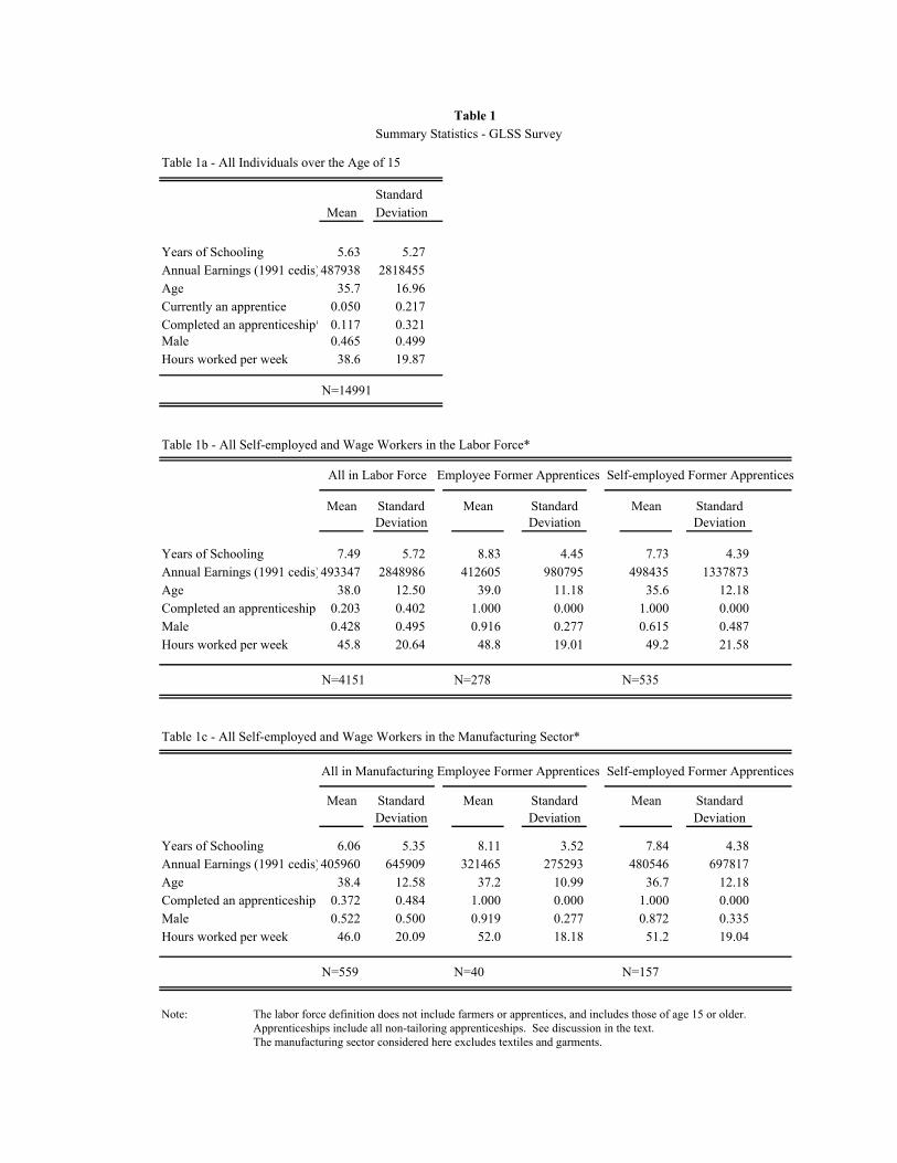
Table 1Summary Statistics - GLSS Survey

Table 1a - All Individuals over the Age of 15

StandardMean Deviation

Years of Schooling 5.63 5.27Annual Earnings (1991 cedis)487938 2818455Age 35.7 16.96Currently an apprentice 0.050 0.217Completed an apprenticeship* 0.117 0.321Male 0.465 0.499Hours worked per week 38.6 19.87

N=14991

Table 1b - All Self-employed and Wage Workers in the Labor Force*

Employee Former Apprentices Self-employed Former Apprentices

Mean Standard Mean Standard Mean StandardDeviation Deviation Deviation

Years of Schooling 7.49 5.72 8.83 4.45 7.73 4.39Annual Earnings (1991 cedis)493347 2848986 412605 980795 498435 1337873Age 38.0 12.50 39.0 11.18 35.6 12.18Completed an apprenticeship 0.203 0.402 1.000 0.000 1.000 0.000Male 0.428 0.495 0.916 0.277 0.615 0.487Hours worked per week 45.8 20.64 48.8 19.01 49.2 21.58

N=4151 N=278 N=535

Table 1c - All Self-employed and Wage Workers in the Manufacturing Sector*

Employee Former Apprentices Self-employed Former Apprentices

Mean Standard Mean Standard Mean StandardDeviation Deviation Deviation

Years of Schooling 6.06 5.35 8.11 3.52 7.84 4.38Annual Earnings (1991 cedis)405960 645909 321465 275293 480546 697817Age 38.4 12.58 37.2 10.99 36.7 12.18Completed an apprenticeship 0.372 0.484 1.000 0.000 1.000 0.000Male 0.522 0.500 0.919 0.277 0.872 0.335Hours worked per week 46.0 20.09 52.0 18.18 51.2 19.04

N=559 N=40 N=157

Note: The labor force definition does not include farmers or apprentices, and includes those of age 15 or older.Apprenticeships include all non-tailoring apprenticeships. See discussion in the text.The manufacturing sector considered here excludes textiles and garments.

All in Labor Force

All in Manufacturing

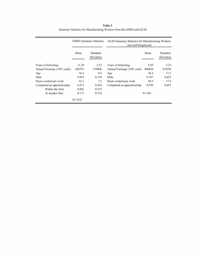
Table 2Summary Statistics for Manufacturing Workers from the GMES and GLSS

GMES Summary Statistics

Mean Standard Mean StandardDeviation Deviation

Years of Schooling 11.20 3.52 Years of Schooling 8.95 5.23Annual Earnings (1991 cedis) 420761 378806 Annual Earnings (1991 cedis) 406820 316299Age 36.4 9.4 Age 36.6 11.2Male 0.853 0.354 Male 0.767 0.425Hours worked per week 43.3 7.5 Hours worked per week 49.5 17.4Completed an apprenticeship 0.251 0.434 Completed an apprenticeship 0.396 0.491

Within this firm 0.081 0.272At another firm 0.171 0.376 N=109

N=2122

GLSS Summary Statistics for Manufacturing Workers(not Self-Employed)

Table 3Activities of Apprentices After Apprenticeship

Fraction of Former Apprentices in Different Activities

Continued working for the firm 0.375Worked for another firm in the industry 0.152Worked for a firm in another industry 0.032Started their own business 0.285School 0.011Unemployed 0.010Don't know 0.178

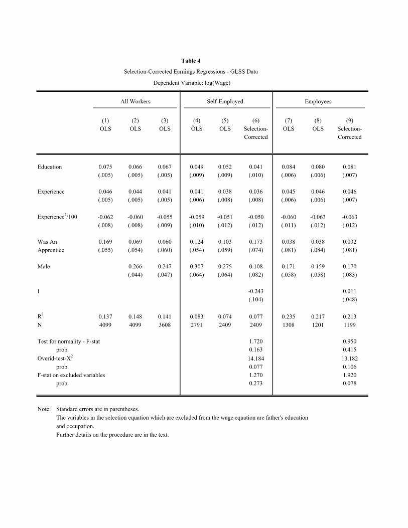
Table 4

Selection-Corrected Earnings Regressions - GLSS Data

Dependent Variable: log(Wage)

All Workers Self-Employed Employees

(1) (2) (3) (4) (5) (6) (7) (8) (9)OLS OLS OLS OLS OLS Selection- OLS OLS Selection-

Corrected Corrected

Education 0.075 0.066 0.067 0.049 0.052 0.041 0.084 0.080 0.081(.005) (.005) (.005) (.009) (.009) (.010) (.006) (.006) (.007)

Experience 0.046 0.044 0.041 0.041 0.038 0.036 0.045 0.046 0.046(.005) (.005) (.005) (.006) (.008) (.008) (.006) (.006) (.007)

Experience2/100 -0.062 -0.060 -0.055 -0.059 -0.051 -0.050 -0.060 -0.063 -0.063(.008) (.008) (.009) (.010) (.012) (.012) (.011) (.012) (.012)

Was An 0.169 0.069 0.060 0.124 0.103 0.173 0.038 0.038 0.032Apprentice (.055) (.054) (.060) (.054) (.059) (.074) (.081) (.084) (.081)

Male 0.266 0.247 0.307 0.275 0.108 0.171 0.159 0.170(.044) (.047) (.064) (.064) (.082) (.058) (.058) (.083)

l -0.243 0.011(.104) (.048)

R2 0.137 0.148 0.141 0.083 0.074 0.077 0.235 0.217 0.213N 4099 4099 3608 2791 2409 2409 1308 1201 1199

Test for normality - F-stat 1.720 0.950prob. 0.163 0.415

Overid-test-X2 14.184 13.182prob. 0.077 0.106

F-stat on excluded variables 1.270 1.920prob. 0.273 0.078

Note: Standard errors are in parentheses. The variables in the selection equation which are excluded from the wage equation are father's educationand occupation.Further details on the procedure are in the text.

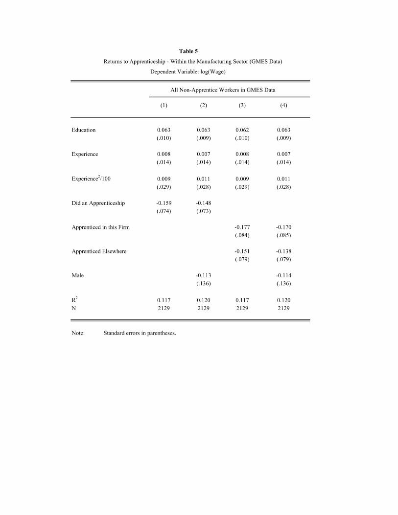
Table 5

Returns to Apprenticeship - Within the Manufacturing Sector (GMES Data)

Dependent Variable: log(Wage)

All Non-Apprentice Workers in GMES Data

(1) (2) (3) (4)

Education 0.063 0.063 0.062 0.063(.010) (.009) (.010) (.009)

Experience 0.008 0.007 0.008 0.007(.014) (.014) (.014) (.014)

Experience2/100 0.009 0.011 0.009 0.011(.029) (.028) (.029) (.028)

Did an Apprenticeship -0.159 -0.148(.074) (.073)

Apprenticed in this Firm -0.177 -0.170(.084) (.085)

Apprenticed Elsewhere -0.151 -0.138(.079) (.079)

Male -0.113 -0.114(.136) (.136)

R2 0.117 0.120 0.117 0.120N 2129 2129 2129 2129

Note: Standard errors in parentheses.

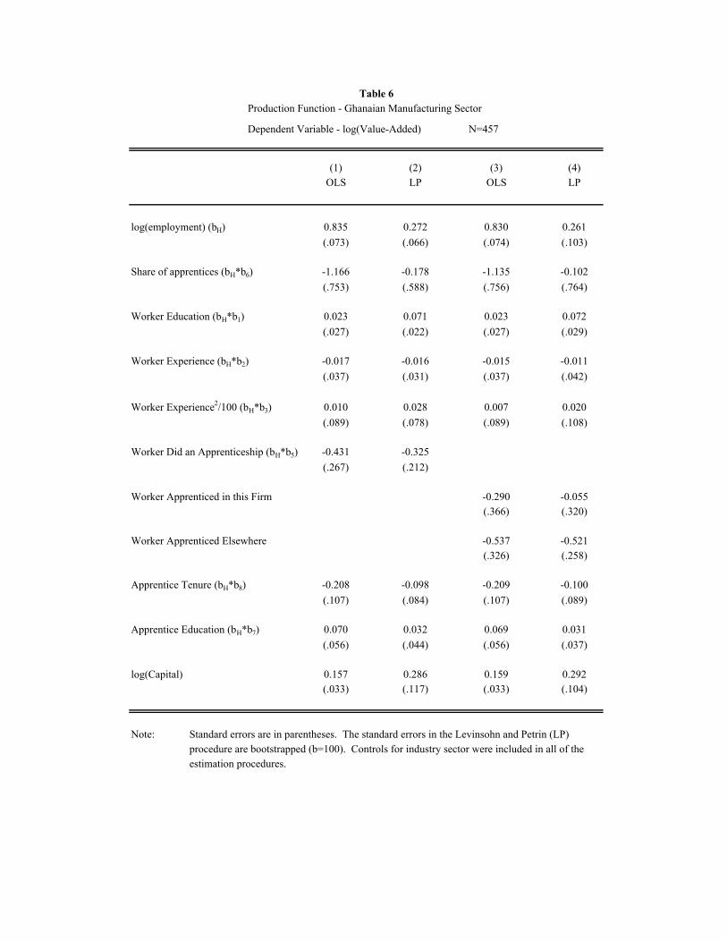
Table 6Production Function - Ghanaian Manufacturing Sector

Dependent Variable - log(Value-Added) N=457

(1) (2) (3) (4)OLS LP OLS LP

log(employment) (bH) 0.835 0.272 0.830 0.261(.073) (.066) (.074) (.103)

Share of apprentices (bH*b6) -1.166 -0.178 -1.135 -0.102(.753) (.588) (.756) (.764)

Worker Education (bH*b1) 0.023 0.071 0.023 0.072(.027) (.022) (.027) (.029)

Worker Experience (bH*b2) -0.017 -0.016 -0.015 -0.011(.037) (.031) (.037) (.042)

Worker Experience2/100 (bH*b3) 0.010 0.028 0.007 0.020(.089) (.078) (.089) (.108)

Worker Did an Apprenticeship (bH*b5) -0.431 -0.325(.267) (.212)

Worker Apprenticed in this Firm -0.290 -0.055(.366) (.320)

Worker Apprenticed Elsewhere -0.537 -0.521(.326) (.258)

Apprentice Tenure (bH*b8) -0.208 -0.098 -0.209 -0.100(.107) (.084) (.107) (.089)

Apprentice Education (bH*b7) 0.070 0.032 0.069 0.031(.056) (.044) (.056) (.037)

log(Capital) 0.157 0.286 0.159 0.292(.033) (.117) (.033) (.104)

Note: Standard errors are in parentheses. The standard errors in the Levinsohn and Petrin (LP)procedure are bootstrapped (b=100). Controls for industry sector were included in all of the estimation procedures.

Appendix Table A1 -First-Stage Probit Estimates of Self-Employment Status

Education -0.086(.008)

Experience -0.011(.006)

Experience2/100 0.010(.009)

Male -1.105(.084)

Did an Apprenticeship 0.346(.068)

Father's SchoolingPrimary -0.180

(.116)

Middle -0.047(.084)

Secondary 0.195(.134)

Father's OccupationFarming -0.115

(.086)

Clerical/Professional -0.179(.096)

Construction -0.177(.163)

N 3610F-stat on excluded variables 2.72p-value on F-stat 0.014

Note: Standard Errors are in Parentheses