Embed Size (px)
Citation preview

Approach from modulus
for Laplace transforms
No.1
Takao Saito
1

Thank you for our world
2

Approach from modulus
for Lapalace transforms
3
Preface
This paper is builded by three parts. First is representations for
Laplace transforms by modulus. Second is the applications for opera-
tor algebras. Finally, it’s the σ-algebras for Laplace transforms.
Papers
About solvers of differential equations of relatively
for Laplace transforms
The projection operators for Laplace transforms
The negative condition for Laplace transforms
The ring conditions for Laplace transforms
The field conditions for Laplace transforms
The ring conditions for Now Laplace transforms
The field conditions for Now Laplace transforms
Now, let′s consider with me!
Address
695-52 Chibadera-cho
Chuo-ku Chiba-shi
Postcode 260-0844 Japan
URL: http://opab.web.fc2.com/index.html
(Wed)20.Nov.2013
Takao Saito
4

Contents
Preface
§ Chapter 1
◦ Representation of D(a) and O(a) operations by modulus · · · 7◦ Representation of Y (a) and N(a) operations by modulus · · ·11
◦ Representation of F (a) and −G(a) operations by modulus · · ·15
◦ Representation of T (a) and −S(a) operations by modulus · · ·19
◦ Some results · · · · · · · · · · · · 23
§ Chapter 2
◦ Application to D(a) and O(a) operations · · · · · ·24
◦ Application to Y (a) and N(a) operations · · · · · ·28
◦ Application to F (a) and G(a) operations · · · · · ·33
◦ Application to T (a) and S(a) operations · · · · · ·37
◦ Some results · · · · · · · · · · · · 42
§ Chapter 3
◦ Modulo in e0s or 00 for D(a) operations · · · · · ·43
◦ Modulo in e0s or 00 for Y (a) operations · · · · · ·44
◦ Modulo in e0s or 00 for F (a) operations · · · · · ·46
◦ Modulo in e0s or 00 for T (a) operations · · · · · ·48
◦ Some results · · · · · · · · · · · · 50
5

◦ Conclusion · · · · · · · · · · · · 51
◦ References · · · · · · · · · · · · 52
6
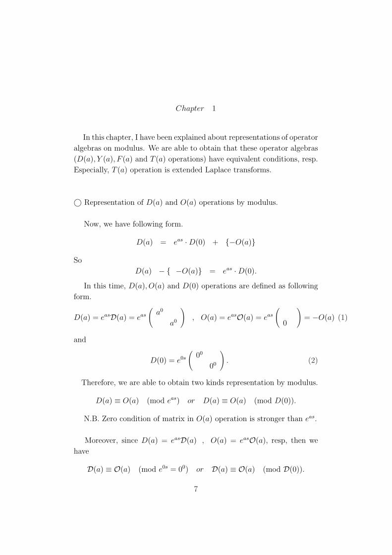
Chapter 1
In this chapter, I have been explained about representations of operator
algebras on modulus. We are able to obtain that these operator algebras
(D(a), Y (a), F (a) and T (a) operations) have equivalent conditions, resp.
Especially, T (a) operation is extended Laplace transforms.
© Representation of D(a) and O(a) operations by modulus.
Now, we have following form.
D(a) = eas ·D(0) + {−O(a)}
So
D(a) − { −O(a)} = eas ·D(0).
In this time, D(a), O(a) and D(0) operations are defined as following
form.
D(a) = easD(a) = eas
(a0
a0
), O(a) = easO(a) = eas
(
0
)= −O(a) (1)
and
D(0) = e0s
(00
00
). (2)
Therefore, we are able to obtain two kinds representation by modulus.
D(a) ≡ O(a) (mod eas) or D(a) ≡ O(a) (mod D(0)).
N.B. Zero condition of matrix in O(a) operation is stronger than eas.
Moreover, since D(a) = easD(a) , O(a) = easO(a), resp, then we
have
D(a) ≡ O(a) (mod e0s = 00) or D(a) ≡ O(a) (mod D(0)).
7
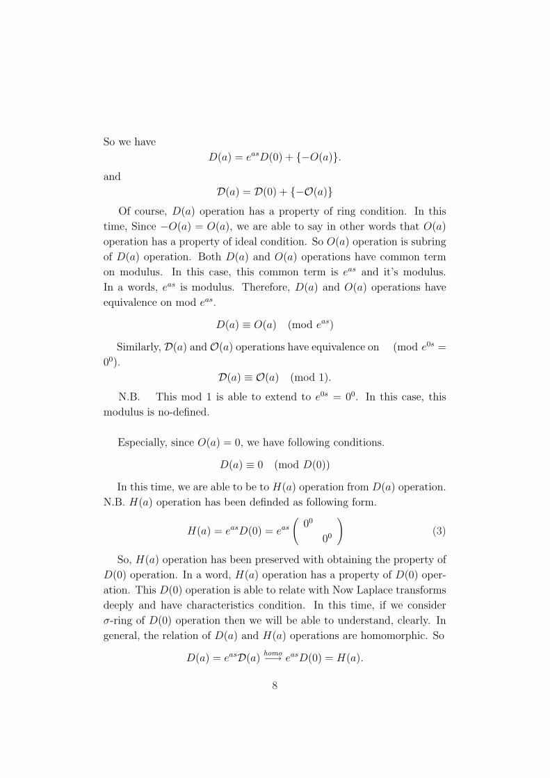
So we have
D(a) = easD(0) + {−O(a)}.and
D(a) = D(0) + {−O(a)}Of course, D(a) operation has a property of ring condition. In this
time, Since −O(a) = O(a), we are able to say in other words that O(a)
operation has a property of ideal condition. So O(a) operation is subring
of D(a) operation. Both D(a) and O(a) operations have common term
on modulus. In this case, this common term is eas and it’s modulus.
In a words, eas is modulus. Therefore, D(a) and O(a) operations have
equivalence on mod eas.
D(a) ≡ O(a) (mod eas)
Similarly, D(a) and O(a) operations have equivalence on (mod e0s =
00).
D(a) ≡ O(a) (mod 1).
N.B. This mod 1 is able to extend to e0s = 00. In this case, this
modulus is no-defined.
Especially, since O(a) = 0, we have following conditions.
D(a) ≡ 0 (mod D(0))
In this time, we are able to be to H(a) operation from D(a) operation.
N.B. H(a) operation has been definded as following form.
H(a) = easD(0) = eas
(00
00
)(3)
So, H(a) operation has been preserved with obtaining the property of
D(0) operation. In a word, H(a) operation has a property of D(0) oper-
ation. This D(0) operation is able to relate with Now Laplace transforms
deeply and have characteristics condition. In this time, if we consider
σ-ring of D(0) operation then we will be able to understand, clearly. In
general, the relation of D(a) and H(a) operations are homomorphic. So
D(a) = easD(a)homo−→ easD(0) = H(a).
8
Similarly,
D(a)homo−→ D(0) = H(a).
Therefore, the previous special case has inclusion monomorphic be-
tween D(a) and H(a) operations. So
D(a)iso←→ H(a).
Similarly,
D(a)iso←→ H(a).
Clearly, now we have following conditions.
D(a)− {−O(a)} = H(a) = easD(0) or D(a) ≡ O(a) (mod D(0)).
Similarly
D(a) ≡ O(a) (mod D(0)).
This means that the property ofD(a) operation andO(a) operation are
same. In general, D(a) operation has identity. So we will have following
condition.
{1} ≡ {0} (mod D(0))
In this case, since O(a) = 0 then we have D(a) = H(a). This forms
are able to extend on Now Laplace transforms. Furthermore these op-
erations are able to also represent by characteristics condition. Because
D(a) (O(a) = 0) and H(a) operations are containing D(0) operation.
Especially, in this case, D(a) operation is able to consider on D(0) op-
eration. And D(0) operation is possible to be characteristics condition.
This condition has closed relation with Now Laplace transforms and σ-
algebras. And it will generate rings, fields and groups of D(a) and H(a)
operations. For example, the primitive ring (subring) of D(a) operation
is generated by D(0) operation, etc. This relation is able to represent by
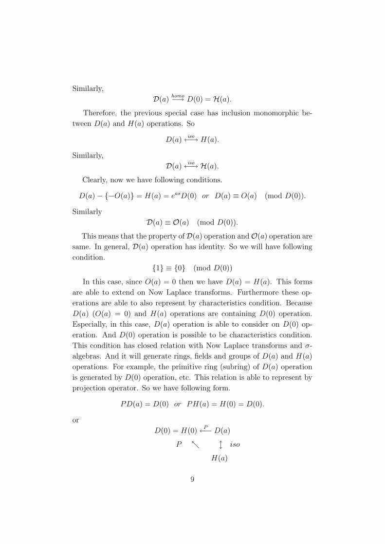
projection operator. So we have following form.
PD(a) = D(0) or PH(a) = H(0) = D(0).
or
D(0) = H(0)P←− D(a)
P ↖ l iso
H(a)
9
N.B. It’s able to consider as isomorphic theorem because of O(a) = 0.
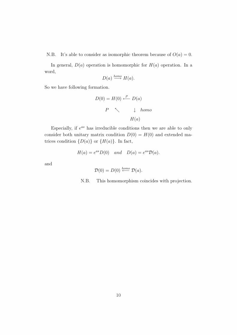
In general, D(a) operation is homomorphic for H(a) operation. In a
word,
D(a)homo−→ H(a).
So we have following formation.
D(0) = H(0)P←− D(a)
P ↖ ↓ homo
H(a)
Especially, if eas has irreducible conditions then we are able to only
consider both unitary matrix condition D(0) = H(0) and extended ma-
trices condition {D(a)} or {H(a)}. In fact,
H(a) = easD(0) and D(a) = easD(a).
and
D(0) = D(0)homo←− D(a).
N.B. This homomorphism coincides with projection.
10
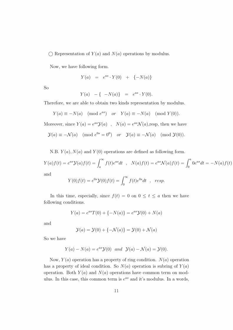
© Representation of Y (a) and N(a) operations by modulus.
Now, we have following form.
Y (a) = eas · Y (0) + {−N(a)}
So
Y (a) − { −N(a)} = eas · Y (0).
Therefore, we are able to obtain two kinds representation by modulus.
Y (a) ≡ −N(a) (mod eas) or Y (a) ≡ −N(a) (mod Y (0)).
Moreover, since Y (a) = easY(a) , N(a) = easN (a),resp, then we have
Y(a) ≡ −N (a) (mod e0s = 00) or Y(a) ≡ −N (a) (mod Y(0)).
N.B. Y (a), N(a) and Y (0) operations are defined as following form.
Y (a)f(t) = easY(a)f(t) =∫ ∞
af(t)easdt , N(a)f(t) = easN (a)f(t) =
∫ a
00easdt = −N(a)f(t) = 0
and
Y (0)f(t) = e0sY(0)f(t) =∫ ∞
0f(t)e0sdt , resp.
In this time, especially, since f(t) = 0 on 0 ≤ t ≤ a then we have
following conditions.
Y (a) = easT (0) + {−N(a)} = easY(0) + N(a)
and
Y(a) = Y(0) + {−N (a)} = Y(0) +N (a)
So we have
Y (a)−N(a) = easY(0) and Y(a)−N (a) = Y(0).
Now, Y (a) operation has a property of ring condition. N(a) operation
has a property of ideal condition. So N(a) operation is subring of Y (a)
operation. Both Y (a) and N(a) operations have common term on mod-
ulus. In this case, this common term is eas and it’s modulus. In a words,
11

eas is modulus. Therefore, Y (a) and N(a) operations have equivalence
on mod eas. Therefore
Y (a) ≡ N(a) (mod eas).
Similarly, Y(a) andN (a) operations have equivalence on (mod e0s =
00).
Y(a) ≡ N (a) (mod 1).
N.B. This mod 1 is able to extend to e0s = 00. In this case, this
modulus is no-defined.
Especially, Since N(a) = 0 then we have following conditions.
Y (a) ≡ 0 (mod Y (0))
In this time, we are able to be to W (a) operation from Y (a) operation.
N.B. W (a) operation has been definded as following form.
W (a)f(t) = easY (0)f(t) =∫ ∞
0f(t)easdt.
So, W (a) operation has been preserved with obtaining the property
of Y (0) operation. In a word, W (a) operation has a property of Y (0)
operation. This Y (0) operation is normal integral operation and it has
characteristics condition. In this time, if we consider σ-ring of Y (0) oper-
ation then we will be able to understand, clearly. In general, the relation
of Y (a) and W (a) operations are homomorphic. So
Y (a) = easY(a)homo−→ easY (0) = W (a).
Similarly,
Y(a)homo−→ Y (0) = W(a).
Therefore, the previous special case has inclusion monomorphic be-
tween Y (a) and W (a) operations. So
Y (a)iso←→ W (a).
Similarly,
Y(a)iso←→W(a).
12
Clearly, now we have following conditions.
Y (a)−N(a) = W (a) = easY (0) or Y (a) ≡ N(a) (mod Y (0)).
In this time, since N(a) = 0 then we have Y (a) = W (a). This forms
are applied to extended Now Laplace transforms. Furthermore these op-
erations are able to also represent by characteristics condition. Because
Y (a) (N(a) = 0) and W (a) operations are containing Y (0) operation. In
other words, normal integral operation is able to have the characteristics
condition. Especially, in this case, Y (a) operation is able to be Y (0)
operation. So, Y (a) operation has characteristics condition χ(a). This
condition has closed relation with σ-algebras. And it will generate rings,
fields and groups of Y (a) and W (a) operations. For example, the primi-
tive ring (subring) of Y (a) operation is generated by Y (0) operation, etc.
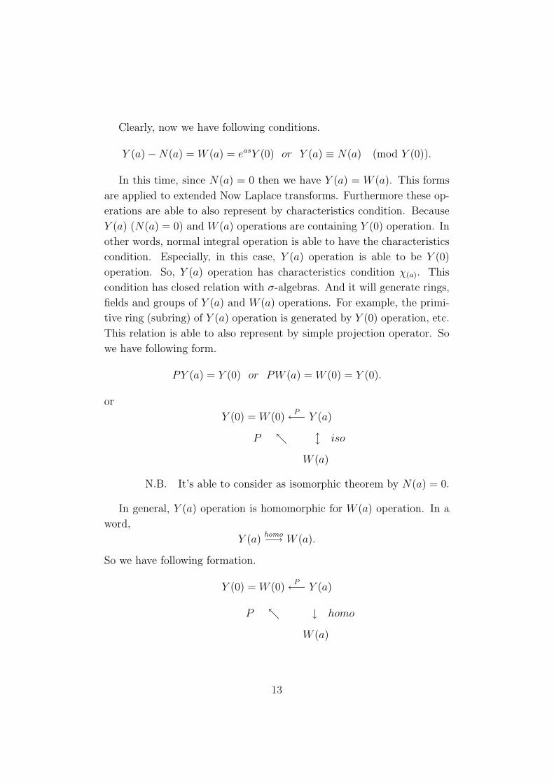
This relation is able to also represent by simple projection operator. So
we have following form.
PY (a) = Y (0) or PW (a) = W (0) = Y (0).
or
Y (0) = W (0)P←− Y (a)
P ↖ l iso
W (a)
N.B. It’s able to consider as isomorphic theorem by N(a) = 0.
In general, Y (a) operation is homomorphic for W (a) operation. In a
word,
Y (a)homo−→ W (a).
So we have following formation.
Y (0) = W (0)P←− Y (a)
P ↖ ↓ homo
W (a)
13
Especially, if eas has irreducible conditions then we are able to only
consider both unitary condition (Y (0) or Y(a)) for Now Laplace trans-
forms {T (0)} and {W (a)} or {Y (a)} operation, resp. In fact,
W (a) = easY (0) and Y (a) = easY(a).
and
Y(0) = Y (0)homo←− Y(a).
N.B. This homomorphism coincides with projection.
14
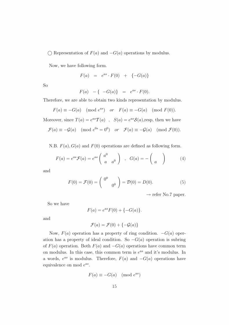
© Representation of F (a) and −G(a) operations by modulus.
Now, we have following form.
F (a) = eas · F (0) + {−G(a)}
So
F (a) − { −G(a)} = eas · F (0).
Therefore, we are able to obtain two kinds representation by modulus.
F (a) ≡ −G(a) (mod eas) or F (a) ≡ −G(a) (mod F (0)).
Moreover, since T (a) = easT (a) , S(a) = easS(a),resp, then we have
F(a) ≡ −G(a) (mod e0s = 00) or F(a) ≡ −G(a) (mod F(0)).
N.B. F (a), G(a) and F (0) operations are defined as following form.
F (a) = easF(a) = eas
(a0
a a0
), G(a) = −
(
a
)(4)
and
F (0) = F(0) =
(00
00
)= D(0) = D(0). (5)
→ refer No.7 paper.
So we have
F (a) = easF (0) + {−G(a)}.and
F(a) = F(0) + {−G(a)}Now, F (a) operation has a property of ring condition. −G(a) oper-
ation has a property of ideal condition. So −G(a) operation is subring
of F (a) operation. Both F (a) and −G(a) operations have common term
on modulus. In this case, this common term is eas and it’s modulus. In
a words, eas is modulus. Therefore, F (a) and −G(a) operations have
equivalence on mod eas.
F (a) ≡ −G(a) (mod eas)
15

Similarly, F(a) and−G(a) operations have equivalence on (mod e0s =
00).
F(a) ≡ −G(a) (mod 1).
N.B. This mod 1 is able to extend to e0s = 00. In this case, this
modulus is no-defined.
In general, since G(a) operation has been ideal then we have following
conditions.
F (a) ≡ 0 (mod F (0))
In this time, we are able to be to H(a) operation from F (a) operation.
N.B. H(a) operation has been definded as following form.
H(a) = easF (0) = eas
(00
00
)= easD(0) = H(a) (6)
So, H(a) operation has been preserved with obtaining the property
of F (0) operation. In a word, H(a) operation has a property of F (0) op-
eration. This F (0) operation is isomorphic with Now Laplace transforms
and it has characteristics condition. In this time, if we consider σ-ring of
F (0) operation then we will be able to understand, clearly. In general,
the relation of F (a) and H(a) operations are homomorphic. So
F (a) = easF(a)homo−→ easF (0) = H(a).
Similarly,
F(a)homo−→ F (0) = H(a).
Therefore, the previous special case has inclusion monomorphic be-
tween F (a) and H(a) operations. So
F (a)iso←→ H(a) iff G(a) = {0}.
Similarly,
F(a)iso←→ H(a) iff G(a) = {0}.
N.B. This {} means set condition. This set condition has related with
σ-algebras.
16
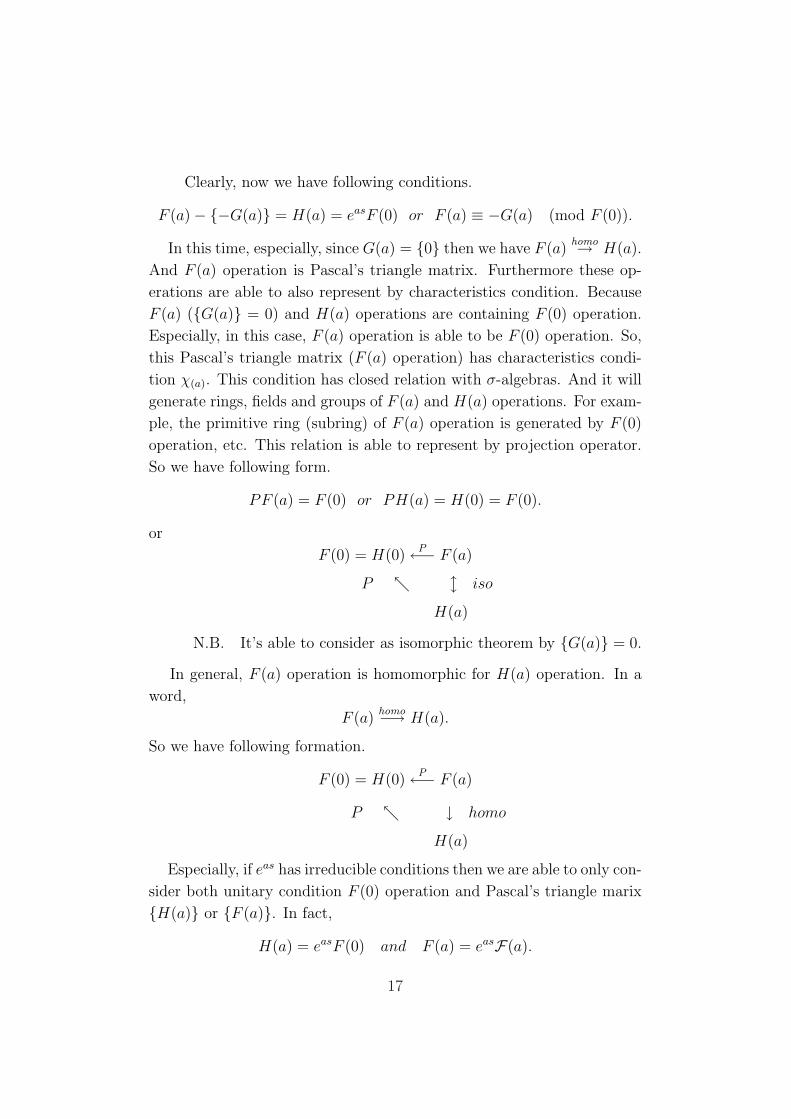
Clearly, now we have following conditions.
F (a)− {−G(a)} = H(a) = easF (0) or F (a) ≡ −G(a) (mod F (0)).
In this time, especially, since G(a) = {0} then we have F (a)homo→ H(a).
And F (a) operation is Pascal’s triangle matrix. Furthermore these op-
erations are able to also represent by characteristics condition. Because
F (a) ({G(a)} = 0) and H(a) operations are containing F (0) operation.
Especially, in this case, F (a) operation is able to be F (0) operation. So,
this Pascal’s triangle matrix (F (a) operation) has characteristics condi-
tion χ(a). This condition has closed relation with σ-algebras. And it will
generate rings, fields and groups of F (a) and H(a) operations. For exam-
ple, the primitive ring (subring) of F (a) operation is generated by F (0)
operation, etc. This relation is able to represent by projection operator.
So we have following form.
PF (a) = F (0) or PH(a) = H(0) = F (0).
or
F (0) = H(0)P←− F (a)
P ↖ l iso
H(a)
N.B. It’s able to consider as isomorphic theorem by {G(a)} = 0.
In general, F (a) operation is homomorphic for H(a) operation. In a
word,
F (a)homo−→ H(a).
So we have following formation.
F (0) = H(0)P←− F (a)
P ↖ ↓ homo
H(a)
Especially, if eas has irreducible conditions then we are able to only con-
sider both unitary condition F (0) operation and Pascal’s triangle marix
{H(a)} or {F (a)}. In fact,
H(a) = easF (0) and F (a) = easF(a).
17

and
F(0) = F (0)homo←− F(a).
N.B. This homomorphism coincides with projection.
18
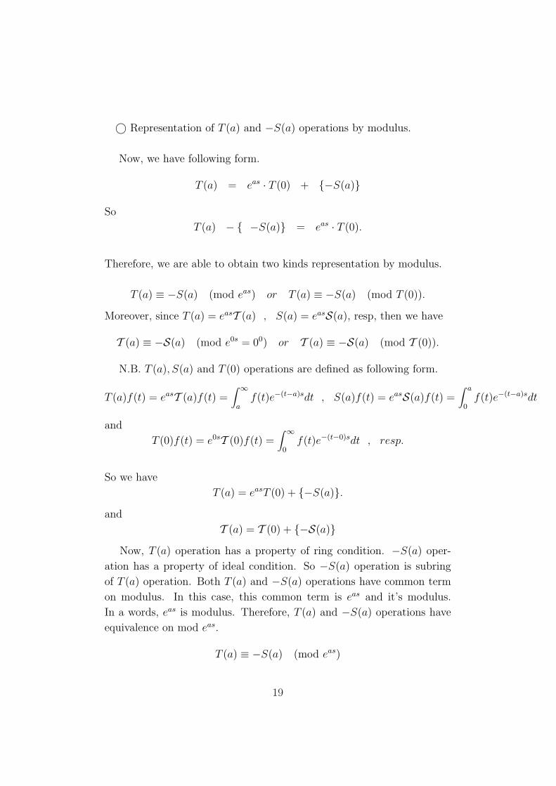
© Representation of T (a) and −S(a) operations by modulus.
Now, we have following form.
T (a) = eas · T (0) + {−S(a)}
So
T (a) − { −S(a)} = eas · T (0).
Therefore, we are able to obtain two kinds representation by modulus.
T (a) ≡ −S(a) (mod eas) or T (a) ≡ −S(a) (mod T (0)).
Moreover, since T (a) = easT (a) , S(a) = easS(a), resp, then we have
T (a) ≡ −S(a) (mod e0s = 00) or T (a) ≡ −S(a) (mod T (0)).
N.B. T (a), S(a) and T (0) operations are defined as following form.
T (a)f(t) = easT (a)f(t) =∫ ∞
af(t)e−(t−a)sdt , S(a)f(t) = easS(a)f(t) =
∫ a
0f(t)e−(t−a)sdt
and
T (0)f(t) = e0sT (0)f(t) =∫ ∞
0f(t)e−(t−0)sdt , resp.
So we have
T (a) = easT (0) + {−S(a)}.and
T (a) = T (0) + {−S(a)}Now, T (a) operation has a property of ring condition. −S(a) oper-
ation has a property of ideal condition. So −S(a) operation is subring
of T (a) operation. Both T (a) and −S(a) operations have common term
on modulus. In this case, this common term is eas and it’s modulus.
In a words, eas is modulus. Therefore, T (a) and −S(a) operations have
equivalence on mod eas.
T (a) ≡ −S(a) (mod eas)
19
Similarly, T (a) and−S(a) operations have equivalence on (mod e0s =
00).
T (a) ≡ −S(a) (mod 1).
N.B. This mod 1 is able to extend to e0s = 00. In this case, this
modulus is no-defined.
Especially, if S(a) = 0 then we have following conditions.
T (a) ≡ 0 (mod T (0))
In this time, we are able to be to R(a) operation from T (a) operation.
N.B. R(a) operation has been definded as following form.
R(a)f(t) = easT (0)f(t) =∫ ∞
0f(t)e−(t−a)sdt.
So, R(a) operation has been preserved with obtaining the property
of T (0) operation. In a word, R(a) operation has a property of T (0)
operation. This T (0) operation is Now Laplace transforms and it has
characteristics condition. In this time, if we consider σ-ring of T (0) oper-
ation then we will be able to understand, clearly. In general, the relation
of T (a) and R(a) operations are homomorphic.
So
T (a) = easT (a)homo−→ easT (0) = R(a).
Similarly,
T (a)homo−→ T (0) = R(a).
Therefore, the previous special case has inclusion monomorphic be-
tween T (a) and R(a) operations.
So
T (a)iso←→ R(a) iff S(a) = 0.
Similarly,
T (a)iso←→R(a) iff S(a) = 0.
20
Clearly, now we have following conditions.
T (a)− {−S(a)} = R(a) = easT (0) or T (a) ≡ −S(a) (mod T (0)).
In this time, especially, if S(a) = 0 then we have T (a) = R(a). This
forms are extended Now Laplace transforms. Furthermore these Laplace
transforms are able to also represent by characteristics condition. Because
T (a) (S(a) = 0) and R(a) operations are containing T (0) operation. Es-
pecially, in this case, T (a) operation is able to be T (0) operation. So, My
Laplace transforms (T (a) operation) has characteristics condition χ(a).
This condition has closed relation with σ-algebras. And it will generate
rings, fields and groups of T (a) and R(a) operations. For example, the
primitive ring (subring) of T (a) operation is generated by T (0) operation,
etc. This relation is able to represent by projection operator. So we have
following form.
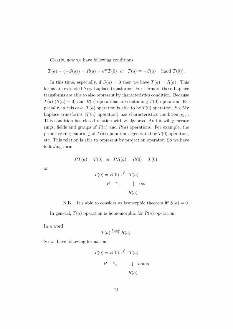
PT (a) = T (0) or PR(a) = R(0) = T (0).
or
T (0) = R(0)P←− T (a)
P ↖ l iso
R(a)
N.B. It’s able to consider as isomorphic theorem iff S(a) = 0.
In general, T (a) operation is homomorphic for R(a) operation.
In a word,
T (a)homo−→ R(a).
So we have following formation.
T (0) = R(0)P←− T (a)
P ↖ ↓ homo
R(a)
21

Especially, if eas has irreducible conditions then we are able to only
consider both unitary condition (Now Laplace transforms {T (0)} and
extended Now Laplace transforms {R(a)} or {T (a)}.
In fact,
R(a) = easT (0) and T (a) = easT (a).
and
T (0) = T (0)homo←− T (a).
N.B. This homomorphism coincides with projection.
22
Some results
◦ Now, T (a) operations obtain two kinds representation by modulus.
T (a) ≡ −S(a) (mod eas) or T (a) ≡ −S(a) (mod T (0)).
N.B. T (0) operation is Now Laplace transforms. So ‖T (0)‖ = 1.
◦ Moreover, since T (a) = easT (a) , S(a) = easS(a), resp, then we have
T (a) ≡ −S(a) (mod e0s = 00) or T (a) ≡ −S(a) (mod T (0)).
◦ The properties of T (a) operation and S(a) operation have same condi-
tions.
◦ We are able to be T (a)iso←→ R(a) iff it’s inclusion monomorphic.
N.B. R(a)def .= easT (0).
◦ The relation of between {1} and {0} is equivalence. Therefore
{1} ≡ {0} (mod T (0))
◦ (mod eas) will treat on C∗-algebras, etc.
23
Chapter 2
In this chapter, I have explained the application to these operator
algebras. In this time, these operator algebras have preserved on a =
0 → ∞ by using (mod e∞s) = (mod e0s). My Hilbert or Banach
spaces are also discussing on this area.
© Application to D(a) and O(a) operations
Now, we have following condition.
D(a) ≡ O(a) (mod e0s = 00)
If a = 0 then we have
D(0) ≡ O(0) (mod e0s = 00).
Similarly, if a = ∞ then we have
D(∞) ≡ O(∞) (mod e0s = 00).
So we are able to have following important condition.
{1} = D(0) ≡ O(0) = {0} = D(∞) ≡ O(∞) = {1} (mod e0s = 00)
N.B. see, No.1, No.11 papers.
Therefore, we obtain
{1} ≡ {0} (mod 00 = e0s).
Since this condition, I have been considered as set condition {1}, {0}.This form is special case for D(a) and O(a) operations. So
D(0) ≡ D(∞) (mod e0s = 00)
24
and
O(0) ≡ O(∞) (mod e0s = 00).
This means that D(0) operation has same property with D(∞). Sim-
ilarly, O(0) operation has same property with O(∞). In a word, D(a)
and O(a) operations are able to discuss on Hilbert spaces.
Similarly, we have following conditions.
D(a) ≡ O(a) (mod eas)
So
D(0) ≡ O(0) (mod e0s = 00)
and
D(∞) ≡ O(∞) (mod e∞s = ∞0)
Now, let’s e0s = e∞s. So we obtain
{1} = D(0) ≡ O(0) = {0} = D(∞) ≡ O(∞) = {1} (mod e0s = e∞s).
Therefore
D(0) ≡ D(∞) (mod e0s = e∞s)
and
O(0) ≡ O(∞) (mod e0s = e∞s).
This means that D(0) operation (a kind of Now Laplace transform)
is preserved by the property of D(∞) operation (a kind of Extended
Laplace transforms). In a words, D(0) operation is able to extend to
D(a) operation.
(see, p.10, No.11)
On the other hand, D(0) operation is able to represent as charactristic
condition χ(0). This characteristic condition has two forms as {1} and
{0}. However, now we have following condition.
{1} ≡ {0} (mod e0s = e∞s).
25
This means that characteristic conditions {1} and {0} are same prop-
erties each other. So we are able to treat two forms equally. For example,
projection operator P and Q have the properties, etc. In other words,
P ≡ Q (mod e0s = 00).
(see, Chapter 1, No.1)
N.B. Q ≡ −Q (mod e0s = 00). Because if P is {1} condition then we
have Q = {0} = −Q. So
P − {−Q} = P −Q = {1}.
Therefore we have previous condition.
Furthermore, we are able to have following conditions.
D(a)iso←→ P , O(a)
iso←→ Q , resp.
So we have,
D(a) ≡ O(a) (mod e0s)
and
D(a) ≡ O(a) (mod eas) or D(a) ≡ O(a) (mod e0s).
This means that D(a) operation has same property for O(a) operation
modulo e0s and D(0) operation.
N.B. H(a) = easD(0) , D(a) + O(a) = H(a) and
(mod eas) = (mod e0s).
Especially, if a is infinite conditions then we have following forms.
(mod e∞s) ≡ (mod e0s).
So we have
D(a) ≡ O(a) (mod e0s = e∞s) for all a.
26
and
D(a) ≡ O(a) (mod e0s = e∞s) for all a.
So we will have following forms.
D(a)iso←→ D(a) , O(a)
iso←→ O(a).
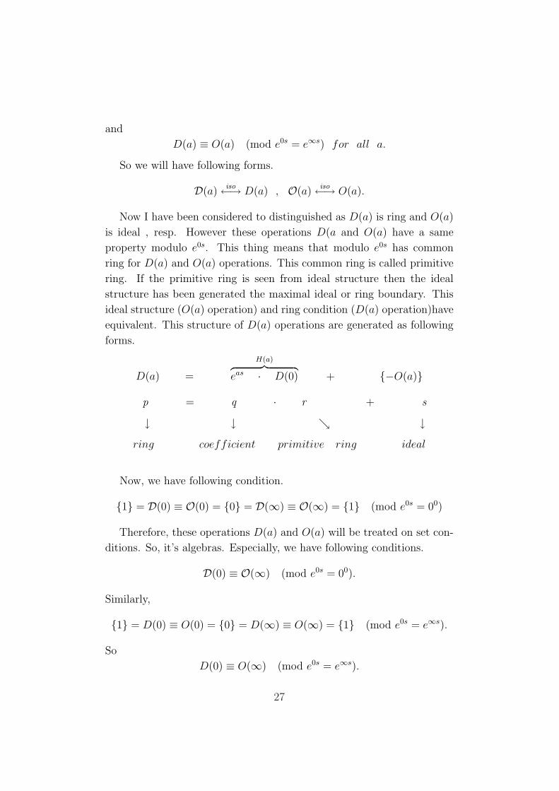
Now I have been considered to distinguished as D(a) is ring and O(a)
is ideal , resp. However these operations D(a and O(a) have a same
property modulo e0s. This thing means that modulo e0s has common
ring for D(a) and O(a) operations. This common ring is called primitive
ring. If the primitive ring is seen from ideal structure then the ideal
structure has been generated the maximal ideal or ring boundary. This
ideal structure (O(a) operation) and ring condition (D(a) operation)have
equivalent. This structure of D(a) operations are generated as following
forms.
D(a) =
H(a)︷ ︸︸ ︷eas · D(0) + {−O(a)}
p = q · r + s
↓ ↓ ↘ ↓ring coefficient primitive ring ideal
Now, we have following condition.
{1} = D(0) ≡ O(0) = {0} = D(∞) ≡ O(∞) = {1} (mod e0s = 00)
Therefore, these operations D(a) and O(a) will be treated on set con-
ditions. So, it’s algebras. Especially, we have following conditions.
D(0) ≡ O(∞) (mod e0s = 00).
Similarly,
{1} = D(0) ≡ O(0) = {0} = D(∞) ≡ O(∞) = {1} (mod e0s = e∞s).
So
D(0) ≡ O(∞) (mod e0s = e∞s).
27
N.B. D(0) = D(0).
On the contrary, we have following conditions.
D(∞) ≡ O(0) (mod e0s = 00).
and
D(∞) ≡ O(0) (mod e0s = e∞s).
N.B. D(∞) = D(∞).
This condition D(0) is applied to Now Laplace transforms. In general,
this operation is extended to ′′a′′ condition. So the operation D(a) is
extended for New Laplace transforms. Essentially, both D(0) and D(a)
operations have same properties. Now, the process of between D(0) and
D(a) operations have only explanation. It is that the operation of between
D(0) operation and D(a) operation has been null condition. In other
words, clearly, it means that O(a) operation has null condition. When it
has this condition, we are able to consider as irreducible condition. In this
case, it is dominated by how to treat the coefficient of D(0) operation.
So it’s that eas is prime number, etc. In this time, in general, we have
following condition.
(mod eas) = (mod e0s).
Therefore the coefficient is characteristics. If e0s has closed condition
then we should that eas also consider on closed condition. On the con-
trary, if e0s has open condition then we should that eas also consider on
open condition. For example, if we consider D(0) and D(∞) operations
only then it will be irreducible condition. In this case, D(a) operations
are possible to generate irreducible conditions between D(0) and D(∞)
operations iff D(a) operation has prime condition.
© Application to Y (a) and N(a) operations
Now, we have following condition.
Y(a) ≡ N (a) (mod e0s)
28
If a = 0 then we have
Y(0) ≡ N (0) (mod e0s = 00).
Similarly, if a = ∞ then we have
Y(∞) ≡ N (∞) (mod e0s = 00).
So we are able to have following important condition.
{1} = Y(0) ≡ N (0) = {0} = Y(∞) ≡ N (∞) = {1}
Therefore, we obtain
{1} ≡ {0} (mod e0s = 00).
Since this condition, I have been considered as set condition {1}, {0}.This form is special case for Y(a) and N (a) operations. So
Y(0) ≡ Y(∞) (mod e0s = 00)
and
N (0) ≡ N (∞) (mod e0s = 00).
This means that Y(0) operation has same property with Y(∞). Sim-
ilarly, N (0) operation has same property with N (∞).
Similarly, we have following conditions.
Y (a) ≡ N(a) (mod eas)
So
Y (0) ≡ N(0) (mod e0s = 00)
and
Y (∞) ≡ N(∞) (mod e∞s = ∞0)
Now, let’s e0s = e∞s. So we obtain
{1} = Y (0) ≡ N(0) = {0} = Y (∞) ≡ N(∞) = {1} (mod e0s = e∞s).
29

Therefore
Y (0) ≡ Y (∞) (mod e0s = e∞s)
and
N(0) ≡ N(∞) (mod e0s = e∞s).
This means that Y (0) operation for Now Laplace transform is pre-
served by the property of Y (∞) operation for Extended Laplace trans-
forms. In a words, Y (0) operation (normal integral operation) is able to
extend to Y (a) operation.
(see, p.14, No.11)
On the other hand, Y (0) operation is able to represent as charactristic
condition χ(0). This characteristics condition is generated from e0s and it
has two forms as {1} and {0}. However, now we have following condition.
{1} ≡ {0} (mod e0s = e∞s).
This means that characteristic conditions {1} and {0} are same prop-
erties each other. So we are able to treat two forms equally. For example,
projection operator P and Q have the properties, etc. In other words,
P ≡ Q (mod e0s = 00).
(see, Chapter 1, No.1)
N.B. Q ≡ −Q (mod e0s = 00). Because, now, we have N(a) = {0}.So we are able to have that Q puts as {0}. In a word,
P − {−Q} = P −Q = {1}.Therefore we have previous condition.
Now, we have following conditions.
Y(a)iso←→ P , N (a)
iso←→ Q , resp.
So we have,
Y(a) ≡ N (a) (mod e0s)
and
Y (a) ≡ N(a) (mod eas) or Y (a) ≡ N(a) (mod e0s).
30

N.B. In this time, N(a) = {0} = −N(a).
This means that Y (a) operation has same property for N(a) oper-
ation modulo e0s and Y (0) operation.
N.B. W (a) = easY (0) , Y (a) + N(a) = W (a) and
(mod eas) = (mod e0s).
Especially, if a is infinite conditions then we have following forms.
(mod e∞s) ≡ (mod e0s).
So we have
Y(a) ≡ N (a) (mod e0s = e∞s) for all a.
and
Y (a) ≡ N(a) (mod e0s = e∞s) for all a.
So we will have following forms.
Y(a)iso←→ Y (a) , N (a)
iso←→ N(a).
Now I have been considered to distinguished as Y (a) is ring and N(a)
is ideal , resp. However these operations Y (a) and N(a) have a same
property modulo e0s. This thing means that modulo e0s has common
ring for Y (a) and N(a) operations. This common ring is called primitive
ring. If the primitive ring is seen from ideal structure then the ideal
structure has been generated the maximal ideal or ring boundary.
Reference
Y (a) =
W (a)︷ ︸︸ ︷eas · Y (0) + {−N(a)}
p = q · r + s
↓ ↓ ↘ ↓ring coefficient primitive ring ideal
31
In general, we are able to be
Y(0)f(t) = N (∞)f(t).
Because of
Y(0)f(t) =∫ ∞
0f(t)dt = N (∞)f(t).
If N (∞) to N(∞) operations then we must have following condition.
Y (0)f(t) = N(∞)f(t) iff e0s = e∞s.
Surely, we have following form.
Y (0)f(t) =∫ ∞
0f(t)e0sdt =
∫ ∞
0f(t)e∞sdt = N(∞)f(t).
Therefore, these operations Y (a) and N(a) will be treated on set
conditions. So, it’s algebras. Especially, in this case, we have following
conditions.
Y(0) = N (∞)
and
Y (0) = N(∞) iff e0s = e∞s.
N.B. Y(0) = Y (0).
This condition Y (0) is applied to Now Laplace transforms. In general,
this operation is extended to ′′a′′ condition. The operation Y (a) is applied
to New Laplace transforms. Essentially, both Y (0) and Y (a) operations
have same properties. Only difference is the process of between Y (0) and
Y (a) operations have two different explanations. One is the operation
of between Y (0) operation and Y (a) operation has been null condition.
In other words, N(a) operation has null condition. When it has this
condition, we are able to consider as irreducible condition. And other is
the operation of between Y (0) operation and Y (a) operation has been
dense condition. In other words, N(a) operation has dense condition.
When it has this condition, we are able to consider as reducible condition.
This classification is dominated by how to treat the coefficient of Y (0)
operation. So it’s eas. In this time, we have following condition.
(mod eas) = (mod e0s).
32

Therefore the coefficient is characteristics. If it has closed condition
then we should consider on irreducible condition. On the contrary, if it
has open condition then we should consider on reducible condition. For
example, if we consider Y (0) and Y (∞) operations only then it will be
irreducible condition and if it also contains with Y (a) (0 < ‖a‖ < ∞)
operation then it will be redicible condition. Of course, Y (a) operation
is possible to also generate irreducible condition between Y (0) operation
iff Y (a) operation has prime conditions.
© Application to F (a) and G(a) operations
Now, we have following condition.
F(a) ≡ −G(a) (mod e0s)
If a = 0 then we have
F(0) ≡ −G(0) (mod e0s = 00).
Similarly, if a = ∞ then we have
F(∞) ≡ −G(∞) (mod e0s = 00).
So we are able to have following important condition.
{1} = F(0) ≡ −G(0) = {0} = F(∞) ≡ −G(∞) = {1}
Therefore, we obtain
{1} ≡ {0} (mod e0s = 00).
Since this condition, I have been considered as set condition {1}, {0}.This form is special case for F(a) and G(a) operations. So
F(0) ≡ F(∞) (mod e0s = 00)
and
−G(0) ≡ −G(∞) (mod e0s = 00).
This means that F(0) operation has same property with F(∞). Sim-
ilarly, −G(0) operation has same property with −G(∞).
33

Similarly, we have following conditions.
F (a) ≡ −G(a) (mod eas)
So
F (0) ≡ −G(0) (mod e0s = 00)
and
F (∞) ≡ −G(∞) (mod e∞s = ∞0)
Now, let’s e0s = e∞s. So we obtain
{1} = F (0) ≡ −G(0) = {0} = F (∞) ≡ −G(∞) = {1} (mod e0s = e∞s).
Therefore
F (0) ≡ F (∞) (mod e0s = e∞s)
and
−G(0) ≡ −G(∞) (mod e0s = e∞s).
This means that F (0) operation is preserved by the property of F (∞)
operation. In a words, unitary of Pascal’s triangle matrix is able to extend
to the F (a) operation.
(see, p.18, No.11)
On the other hand, F (0) operation is able to represent as charactristic
condition χ(0). This characteristic condition has two forms as {1} and
{0}. However, now we have following condition.
{1} ≡ {0} (mod e0s = e∞s).
This means that characteristic conditions {1} and {0} are same prop-
erties each other. So we are able to treat two forms equally. For example,
projection operator P and Q have the properties, etc. In other words,
P ≡ Q (mod e0s = 00).
34
(see, Chapter 1, No.1)
N.B. Q ≡ −Q (mod e0s = 00). Because
Let Q =
(0
1
)(7)
So we have
Q− {−Q} =
(0
1
)−
(0
−1
)= 2
(0
1
)= 2
(00
00
). (8)
Therefore
Q ≡ −Q (mod e0s = 00).
Now, we have following conditions.
F(a)homo−→ P , G(a)
homo−→ Q , resp.
Moreover, F(a) and G(a) operations have a property of inclusion
monomorphism for projection operators. So we have,
F(a) ≡ G(a) (mod e0s)
and
F (a) ≡ G(a) (mod eas) or F (a) ≡ G(a) (mod e0s).
This means that F (a) operation has same property for G(a) operation
modulo e0s and F (0) operation.
N.B. H(a) = easF (0) , F (a) + G(a) = H(a) and
(mod eas) = (mod e0s).
Especially, if a is infinite conditions then we have following forms.
(mod e∞s) ≡ (mod e0s).
So we have
F(a) ≡ G(a) (mod e0s = e∞s) for all a.
35

and
F (a) ≡ G(a) (mod e0s = e∞s) for all a.
So we will have following forms.
F(a)iso←→ F (a) , G(a)
iso←→ G(a).
Now I have been considered to distinguished as F (a) is ring and G(a)
is ideal , resp. However these operations F (a) and G(a) have a same
property modulo e0s. This thing means that modulo e0s has common
ring for F (a) and G(a) operations. This common ring is called primitive
ring. If the primitive ring is seen from ideal structure then the ideal
structure has been generated the maximal ideal or ring boundary.
Reference
F (a) =
H(a)︷ ︸︸ ︷eas · F (0) + {−G(a)}
p = q · r + s
↓ ↓ ↘ ↓ring coefficient primitive ring ideal
In this time, we are able to be following condition.
F(0) = G(∞)
and
F (0) = G(∞) iff e0s = e∞s.
N.B. T (0) = T (0).
For example,
‖F(0)‖ = ‖(
00
00
)‖ = ‖00‖ = 1 = ‖ −
(
∞
)‖ = ‖G(∞)‖. (9)
So we have
F(0) = G(∞).
36
N.B. F(0) = F (0) = D(0) = D(0).
This condition F (0) is treated on diagonal conditions for Pascal’s
triangle matrix. In general, this operation is extended to ′′a′′ condition.
The operation F (a) is Pascal’s triangle matrix. Essentially, both F (0) and
F (a) operations have same properties. Only difference is the process of
between F (0) and F (a) operations have two different explanations. One
is the operation of between F (0) operation and F (a) operation has been
null condition. In other words, G(a) operation has null condition (G(a) =
{0}). When it has this condition, we are able to consider as irreducible
condition. And other is the operation of between F (0) operation and F (a)
operation has been dense condition. In other words, G(a) operation has
dense condition. When it has this condition, we are able to consider as
reducible condition. This classification is dominated by how to treat the
coefficient of F (0) operation. So it’s eas. In this time, we have following
condition.
(mod eas) = (mod e0s).
Therefore the coefficient is characteristics. If it has closed condition
then we should consider on irreducible condition. On the contrary, if it
has open condition then we should consider on reducible condition. For
example, if we consider F (0) and F (∞) operations only then it will be
irreducible condition and if it also contains with F (a) (0 < ‖a‖ < ∞)
operation then it will be redicible condition. Of course, F (a) operation
is possible to also generate irreducible condition between F (0) operation
iff F (a) operation has prime conditions.
© Application to T (a) and S(a) operations
Now, we have following condition.
T (a) ≡ −S(a) (mod e0s)
If a = 0 then we have
T (0) ≡ −S(0) (mod e0s = 00).
Similarly, if a = ∞ then we have
T (∞) ≡ −S(∞) (mod e0s = 00).
37
So we are able to have following important condition.
{1} = T (0) ≡ −S(0) = {0} = T (∞) ≡ −S(∞) = {1} (mod e0s = 00)
Therefore, we obtain
{1} ≡ {0} (mod e0s = 00).
Since this condition, I have been considered as set condition {1}, {0}.This form is special case for T (a) and S(a) operations. So
T (0) ≡ T (∞) (mod e0s = 00)
and
−S(0) ≡ −S(∞) (mod e0s = 00).
This means that T (0) operation has same property with T (∞). Sim-
ilarly, −S(0) operation has same property with −S(∞). In a word, T (a)
and S(a) operations are able to discuss on Hilbert spaces.
Similarly, we have following conditions.
T (a) ≡ −S(a) (mod eas)
So
T (0) ≡ −S(0) (mod e0s = 00)
and
T (∞) ≡ −S(∞) (mod e∞s = ∞0)
Now, let’s e0s = e∞s. So we obtain
{1} = T (0) ≡ −S(0) = {0} = T (∞) ≡ −S(∞) = {1} (mod e0s = e∞s).
Therefore
T (0) ≡ T (∞) (mod e0s = e∞s)
and
−S(0) ≡ −S(∞) (mod e0s = e∞s).
This means that T (0) operation (Now Laplace transform) is preserved
by the property of T (∞) operation (Extended Laplace transforms). In a
words, Now Laplace transform is able to extend to T (a) operation.
38

(see, p.22, No.11)
On the other hand, T (0) operation is able to represent as charactristic
condition χ(0). This characteristic condition has two forms as {1} and
{0}. However, now we have following condition.
{1} ≡ {0} (mod e0s = e∞s).
This means that characteristic conditions {1} and {0} are same prop-
erties each other. So we are able to treat two forms equally. For example,
projection operator P and Q have the properties, etc. In other words,
P ≡ Q (mod e0s = 00).
(see, Chapter 1, No.1)
N.B. Q ≡ −Q (mod e0s = 00). Because
Let Q =
(0
1
)(10)
So we have
Q− {−Q} =
(0
1
)−
(0
−1
)= 2
(0
1
)= 2
(00
00
). (11)
Therefore
Q ≡ −Q (mod e0s = 00).
Now, we have following conditions.
T (a)homo−→ P , S(a)
homo−→ Q , resp.
Moreover, T (a) and S(a) operations have a property of inclusion
monomorphism for projection operators. So we have,
T (a) ≡ S(a) (mod e0s)
and
T (a) ≡ S(a) (mod eas) or T (a) ≡ S(a) (mod e0s).
39
This means that T (a) operation has same property for S(a) operation
modulo e0s and T (0) operation.
N.B. R(a) = easT (0) , T (a) + S(a) = R(a) and
(mod eas) = (mod e0s).
Especially, if a is infinite conditions then we have following forms.
(mod e∞s) ≡ (mod e0s).
So we have
T (a) ≡ S(a) (mod e0s = e∞s) for all a.
and
T (a) ≡ S(a) (mod e0s = e∞s) for all a.
So we will have following forms.
T (a)iso←→ T (a) , S(a)
iso←→ S(a).
Now I have been considered to distinguished as T (a) is ring and S(a) is
ideal , resp. However these operations T (a and S(a) have a same property
modulo e0s. This thing means that modulo e0s has common ring for T (a)
and S(a) operations. This common ring is called primitive ring. If the
primitive ring is seen from ideal structure then the ideal structure has
been generated the maximal ideal or ring boundary.
(see, P.55, No.10)
Clearly,
T (0)f(t) = S(∞)f(t).
Because of
T (0)f(t) =∫ ∞
0f(t)e−stdt = S(∞)f(t).
If S(∞) to S(∞) operations then we must have following condition.
T (0)f(t) = S(∞)f(t) iff e0s = e∞s.
40
Surely, we have following form.
T (0)f(t) =∫ ∞
0f(t)e−(t−0)sdt =
∫ ∞
0f(t)e−(t−∞)sdt = S(∞)f(t).
Therefore, these operations T (a) and S(a) will be treated on set con-
ditions. So, it’s algebras. Especially, in this case, we have following
conditions.
T (0) = S(∞)
and
T (0) = S(∞) iff e0s = e∞s.
N.B. T (0) = T (0).
This condition T (0) is treated on Now Laplace transforms. In gen-
eral, this operation is extended to ′′a′′ condition. The operation T (a) is
extended to New Laplace transforms. Essentially, both T (0) and T (a) op-
erations have same properties. Only difference is the process of between
T (0) and T (a) operations have two different explanations. One is the
operation of between T (0) operation and T (a) operation has been null
condition. In other words, S(a) operation has null condition. When it
has this condition, we are able to consider as irreducible condition. And
other is the operation of between T (0) operation and T (a) operation has
been dense condition. In other words, S(a) operation has dense condi-
tion. When it has this condition, we are able to consider as reducible
condition. This classification is dominated by how to treat the coefficient
of T (0) operation. So it’s eas. In this time, we have following condition.
(mod eas) = (mod e0s).
Therefore the coefficient is characteristics. If it has closed condition
then we should consider on irreducible condition. On the contrary, if it
has open condition then we should consider on reducible condition. For
example, if we consider T (0) and T (∞) operations only then it will be
irreducible condition and if it also contains with T (a) (0 < ‖a‖ < ∞)
operation then it will be redicible condition. Of course, T (a) operation
is possible to also generate irreducible condition between T (0) operation
iff T (a) operation has prime conditions.
41

Some results
◦ Now we have following condition.
{1} = T (0) ≡ −S(0) = {0} = T (∞) ≡ −S(∞) = {1} (mod e0s = e∞s).
So
{1} ≡ {0} (mod e0s = e∞s).
◦ Projection operators have following property.
P ≡ Q (mod e0s = 00).
◦ Laplace transforms have modulo with the ideal structures. So
T (a) ≡ S(a) (mod eas).
◦ Especially, we have following conditions, now.
(mod eas) = (mod e0s = 00).
◦ Clearly, T (0) operation is equal with S(∞). (L2-spaces)
T (0) ≡ S(∞) (mod e0s = 00).
and
S(0) ≡ T (∞) (mod e0s = 00).
◦ Similarly,
T (0) ≡ S(∞) (mod e0s = e∞s).
and
S(0) ≡ T (∞) (mod e0s = e∞s).
42
Chapter 3
In this chapter, I want to explain about the modulo in e0s = 00. This
form is able to be characteristics conditions. This condition is related with
σ-algebras, deeply close. These operator algebras was extended from this
condition.
© Modulo in e0s or 00 for D(a) operations
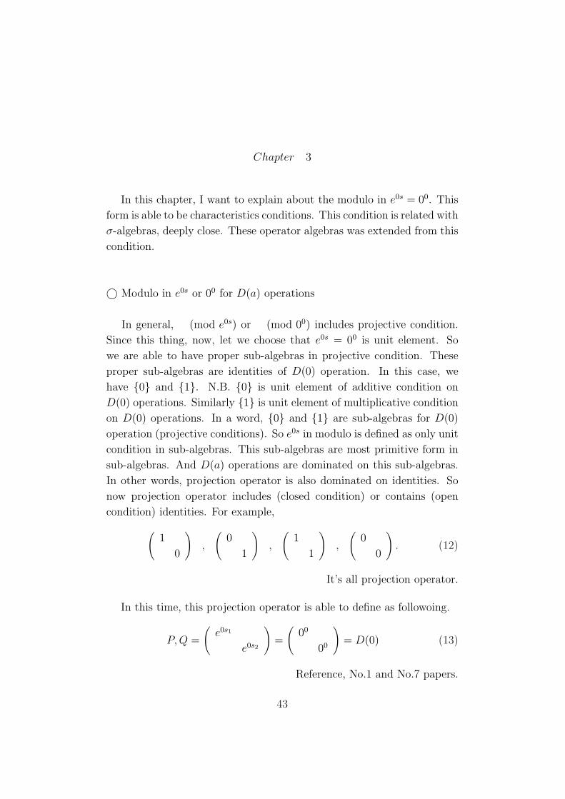
In general, (mod e0s) or (mod 00) includes projective condition.
Since this thing, now, let we choose that e0s = 00 is unit element. So
we are able to have proper sub-algebras in projective condition. These
proper sub-algebras are identities of D(0) operation. In this case, we
have {0} and {1}. N.B. {0} is unit element of additive condition on
D(0) operations. Similarly {1} is unit element of multiplicative condition
on D(0) operations. In a word, {0} and {1} are sub-algebras for D(0)
operation (projective conditions). So e0s in modulo is defined as only unit
condition in sub-algebras. This sub-algebras are most primitive form in
sub-algebras. And D(a) operations are dominated on this sub-algebras.
In other words, projection operator is also dominated on identities. So
now projection operator includes (closed condition) or contains (open
condition) identities. For example,
(1
0
),
(0
1
),
(1
1
),
(0
0
). (12)
It’s all projection operator.
In this time, this projection operator is able to define as followoing.
P,Q =
(e0s1
e0s2
)=
(00
00
)= D(0) (13)
Reference, No.1 and No.7 papers.
43

For example, F(a) operation has defined as following form.
F(a) =
(a0
a a0
)(14)
If a → 0 then we have projective condition. This thing means that
F(0) = D(0) generates as σ-algebras. In a word, D(0) is a kind of σ-
algebras. N.B. F(0) = D(0). This D(0) operation has deep relartion
with Now Laplace transforms. In a word, D(0) has been generated σ-
algebras and especially, Now Laplace transform has been generated iden-
tities in this σ-algebras. These identities are called primitive or proper
sub-algebras. The σ-algebras are dominated on these identities. For ex-
ample,
{0} =
(0
0
),
(1
0
),
(0
1
),
(1
1
)= {1} (15)
N.B. It’s all σ-algebra. Especially, {0}, {1} are identities.
Now, we have following conditions.
D(0) = {1} = O(∞) and O(0) = {0} = D(∞)
I was treated these conditions for convenience until now. If this iden-
tities treat on set condition of {0} and {1} then we have following con-
ditions, easier.
D(0) ≡ D(∞) (mod e0s)
and
O(∞) ≡ O(0) (mod e0s).
By {0} ≡ {1} (mod e0s).
These things are treated on L2 and L1-spaces, etc.
Refer No.1 and No.11 papers.
© Modulo in e0s or 00 for Y (a) operations
In general, (mod e0s) or (mod 00) includes projective condition.
44
Since this thing, now, let we choose that e0s = 00 is unit element. So
we are able to have proper sub-algebras in projective condition. These
proper sub-algebras are normal integral operator Y (0) for Now Laplace
transforms. In this case, we have {0} and {1}. N.B. {0} is unit element
of additive condition on Y (0) operation. Similarly {1} is unit element of
multiplicative condition on Y (0) operation. In a word, {0} and {1} are
sub-algebras for Y (0) operation (projective conditions). So e0s in modulo
is defined as only unit condition in sub-algebras. This sub-algebras are
most primitive form in sub-algebras. And Y (a) operation is dominated on
this sub-algebras. In other words, projection operator is also dominated
on identities. So now projection operator includes (closed condition) or
contains (open condition) identities. For example,
(1
0
),
(0
1
),
(1
1
),
(0
0
). (16)
It’s all projection operator.
In this time, this projection operator is able to define as followoing.
P, Q =
(e0s1
e0s2
)=
(00
00
)iso↔ Y (0) (17)
Reference, No.1 and No.7 papers.
For example, D(a) operation has defined as following form.
D(a) =
(a0
a0
)(18)
If a → 0 then we have projective condition. This thing means that
D(0) generates as σ-ring. In a word, Y (0) is a kind of σ-ring. N.B.
D(0)iso↔ Y (0). Hahn’s decomposition is able to apply to these Y (0) or
Y (a) operations. On condition that these forms generate the characteris-
tics condition on Y (0) or Y (a) operations. N.B. Y (0) or Y (a) operations
are defined as following forms, resp.
Y (0)f(t) =∫ ∞
0f(t)e0sdt or Y (a)f(t) =
∫ ∞
af(t)easdt.
45
If t = 0 then the kernel of Y (0) operation generates the characteristics
condition. In general, if t = a condition then we have N(a) operation on
0 ≤ t ≤ a and Y (a) operation on a ≤ t ≤ ∞. Now, since N(a) ≡ Y (a)
(mod e0s) then N(a) and Y (a) operations at t = a also have important
conditions (characteristics). These things means that Y (0) and Y (a) op-
erations have a same properties on 0 and a, resp. So Y (a) operation is
same condition with Y (0) operation (normal integral operators). There-
fore it has same situations even if extended conditions Y (a). In other
words, all operations that it’s generated on a = 0 are able to treat on ′′a′′
condition, samely.
Now, we have following conditions.
Y(0) = {1} = N (∞) and N (0) = {0} = Y(∞)
I was treated these conditions for convenience until now. If this identities
treat on set condition of {0} and {1} then we have following conditions,
easier.
Y(0) ≡ Y(∞) (mod e0s)
and
N (∞) ≡ N (0) (mod e0s).
By {0} ≡ {1} (mod e0s).
These things are treated on L2 and L1-spaces, etc.
Refer No.1 and No.11 papers.
© Modulo in e0s or 00 for F (a) operations
In general, (mod e0s) or (mod 00) includes projective condition.
Since this thing, now, let we choose that e0s = 00 is unit element. So we
are able to have proper sub-algebras in projective condition. These proper
sub-algebras are identities for Pascal’s triangle matrix (F (a) operation).
In this case, we have {0} and {1}. N.B. {0} is unit element of additive
condition on Pascal’s triangle matrix. Similarly {1} is unit element of
multiplicative condition on Pascal’s triangle matrix. In a word, {0} and
46

{1} are proper sub-algebras for it if a = 0 (projective conditions). So
minimum e0s in modulo is defined as only unit condition in sub-algebras.
This sub-algebras are most primitive form in sub-algebras. And Pascal’s
triangle matrix is dominated on this sub-algebras. In other words, projec-
tion operator is also dominated on identities. So now projection operator
includes (closed condition) or contains (open condition) identities. For
example,
(1
0
),
(0
1
),
(1
1
),
(0
0
). (19)
It’s all projection operator.
In this time, this projection operator is able to define as followoing.
P, Q =
(e0s1
e0s2
)=
(00
00
)= F (0). (20)
Reference, No.1 and No.7 papers.
In this time, F(a) operation has defined as following form.
F(a) =
(a0
a a0
)(21)
If a → 0 then we have projective condition. This thing means
that F(0) generates as σ-ring. Furthermore, T (0) is a kind of σ-ring.
N.B. F(0)iso↔ T (0). Hahn’s decomposition is able to apply to these
F (0) or F (a) operations. On condition that these forms generate the
characteristics condition on F (0) or F (a) operations. N.B. F (0) or F (a)
operations are defined as following forms, resp.
F (0) =
(00
00
), F (a) = eas
(a0
a a0
)(22)
Now, we have
F (0) ≡ G(∞) (mod e0s = e∞s)
So the property of F (0) and G(∞) is same. In this case, the charac-
teristics condition exists on 0 ≤ a ≤ ∞.
47
Now, we are able to obtain following conditions.
F(0) = {1} = G(∞) and G(0) = {0} = F(∞)
I was treated these conditions for convenience until now. If this iden-
tities treat on set condition of {0} and {1} then we have following con-
ditions, easier.
F(0) ≡ F(∞) (mod e0s)
and
G(∞) ≡ G(0) (mod e0s).
By {0} ≡ {1} (mod e0s).
These things are treated on L2 and L1-spaces, etc.
Refer No.1 and No.11 papers.
© Modulo in e0s or 00 for T (a) operations
In general, (mod e0s) or (mod 00) includes projective condition.
Since this thing, now, let we choose that e0s = 00 is unit element. So we
are able to have proper sub-algebras in projective condition. These proper
sub-algebras are Now Laplace transforms. In this case, we have {0} and
{1}. N.B. {0} is unit element of additive condition on Now Laplace
transforms. Similarly {1} is unit element of multiplicative condition on
Now Laplace transforms. In a word, {0} and {1} are sub-algebras for
extended Laplace transforms (projective conditions). So e0s in modulo
is defined as only unit condition in sub-algebras. This sub-algebras are
most primitive form in sub-algebras. And extended Laplace transforms
are dominated on this sub-algebras. In other words, projection operator is
also dominated on identities. So now projection operator includes (closed
condition) or contains (open condition) identities. For example,
(1
0
),
(0
1
),
(1
1
),
(0
0
). (23)
It’s all projection operator.
48
In this time, this projection operator is able to define as followoing.
P,Q =
(e0s1
e0s2
)=
(00
00
)(24)
Reference, No.1 and No.7 papers.
Moreover, F(a) operation has defined as following form.
F(a) =
(a0
a a0
)(25)
If a → 0 then we have projective condition. This thing means that
F(0) generates as σ-ring. In a word, T (0) is a kind of σ-ring. N.B.
F(0)iso↔ T (0). So F(0) operation has a characteristics condition. Hahn’s
decomposition is able to apply to these T (0) or T (a) operations on condi-
tion that these forms also generate the characteristics condition at t = 0
or t = a, resp. Because of the kernel of T (0) or T (a) operations generates
e0s = 00. N.B. T (0) or T (a) operations are defined as following forms.
T (0)f(t) =∫ ∞
0f(t)e−(t−0)sdt or T (a)f(t) =
∫ ∞
af(t)e−(t−a)sdt.
And if t = a condition then we have S(a) operation on 0 ≤ t ≤ a and T (a)
operation on a ≤ t ≤ ∞. Now, since S(a) ≡ T (a) (mod e0s) then S(a)
and T (a) operations at t = a have important conditions (characteristics).
Now, we have following conditions.
T (0) = {1} = S(∞) and S(0) = {0} = T (∞)
I was treated these conditions for convenience until now. If this iden-
tities treat on set condition of {0} and {1} then we have following con-
ditions, easier.
T (0) ≡ T (∞) (mod e0s)
and
S(∞) ≡ S(0) (mod e0s).
By {0} ≡ {1} (mod e0s).
These things are treated on L2 and L1-spaces, etc.
Refer No.1 and No.11 papers.
49
Some results
◦ Now Laplace transforms have been generated from identities {1}, {0}.
◦ Now Laplace transform is the smallest algebras in operator algebras.
◦ e0s and 00 have characteristics conditions, resp. The situations generate
Now Laplace transforms.
◦ σ-algebra is able to represent the projection operator.
◦ Extended Laplace transforms are isomorphic with the projection oper-
ator.
◦ Now Laplace transforms and Extended Laplace transforms have same
properties. So we have following conditions.
T (0) ≡ T (∞) (mod e0s)
by {1} ≡ {0} (mod e0s).
50
Conclusion
Now, T (a) operations are able to represent as algebraic forms. So
we are able to have certain forms by modulo conditions. This modulo
conditions have two kinds forms. One is eas and other is T (0). eas of
modulo conditions has been used on the assertion of extended conditions
for operator algebras. On the other hand, T (0) of modulo conditions has
been used on assertion of Now Laplace transforms. The characteristics
of T (0) operation are represent as e0s. So, both eas and T (0) have same
modulus by
(mod eas) = (mod e0s).
In this time, we have following conditions.
T (a) ≡ S(a) (mod eas) or T (a) ≡ S(a) (mod T (0)).
This means that extended Laplace transforms (T (a) operation) and
the ideal structures (S(a) operation) have same properties by modulo eas
or T (0) operation. In a word, T (0) operation becomes sub-algebras on
T (a) and S(a) operations. In fact, T (0) operation is the smallest algebras
in T (a) and S(a) operations. So T (0) operation (Now Laplace transform)
is identity. But, now, we should attend to T (0) operation. In fact, if we
extend our consideration then T (0) operation has chatacteristics condi-
tion. So, we are able to extend to σ-algebras. In this time, T (a) operation
and T (0) operation are same conditions. Precisely speaking,
PT (a) = T (0).
The next time, we have
{1} = T (0) ≡ −S(0) = {0} = T (∞) ≡ −S(∞) = {1} (mod e0s = e∞s).
So we have,
{1} ≡ {0} (mod e0s = e∞s).
In this time, if we consider as T (a) and S(a) operations are set con-
ditions then we are able to obtain the algebraic forms. These forms are
able to be ring, field, and group on Laplace transforms.
(Wed)20.Nov.2013
Now, let′s go to next papers with me!
51
References
[1] Bryan P.Rynne and Martin A.Youngson,Springer, SUMS, Linear func-
tional analysis,Springer, SUMS, 2001.
[2] Micheal O Searcoid, Elements of Abstract Analysis, Springer, SUMS,
2002.
[3] Israel Gohberg and Seymour Goldberg, Basic operator theory,
Birkhauser, 1980.
[4] Harry Hochtadt, Integral Equations, John & Sons,Inc, 1973.
[5] P.M.Cohn, Springer, SUMS, An Introduction to Ring Theory.
[6] M.A.Naimark, Normed Rings, P.Noordhoff,Ltd, 1959.
[7] Emil G.Milewski, Rea’s Problem Solvers Topology, 1998.
Furthermore
[8] Kosaku Yoshida, Functional Analysis, Springer, 1980.
[9] Irina V.Melnikova, Abstract Cauchy problems, Chapman, 2001.
[10] Paul L.Butzer Hubert Berens, Semi-groups of Operators and Ap-
proximation, Springer, 1967
[11] Hille and Philips, Functional analysis and semi-Groups, AMS, 1957.
[12] Richard V. Kadison John R.Ringrose Fundamentals of the theory of
Operator Algebras, AMS
[13] Dunford & Schwartz Linear operators I,II,III, Wiley.
[14] Charles E.Rickart, General theory of Banach algebras, D.Van Nos-
trand Company,Inc,1960.
[15] J.L.Kelley · Isaac Namioka Linear topological spaces, D.Van Nos-
trand Company,Inc, 1961.
[16] Gareth A.Jones and J.Mary Jones, Elementary number theory,
Springer, 2006.
52