Embed Size (px)
Citation preview

Received April 1, 2015 Accepted as Economics Discussion Paper April 2, 2015 Published April 9, 2015
© Author(s) 2015. Licensed under the Creative Commons License - Attribution 3.0
Discussion PaperNo. 2015-25 | April 09, 2015 | http://www.economics-ejournal.org/economics/discussionpapers/2015-25
Please cite the corresponding Journal Article athttp://www.economics-ejournal.org/economics/journalarticles/2015-43
FTA Effects on Agricultural Trade with MatchingApproaches
GaSeul Lee and Song Soo Lim
AbstractWhile the trade effect of free trade agreements (FTAs) is a global issue, little research has examinedthe economic effects of trade liberalization on agricultural products with robust empirical methods.In this study, propensity score matching for controlling selection bias is used to examine andanalyze the effect of FTAs on the trade of South Korea’s agricultural products. To enhance therobustness of estimated results, differences between the FTA treatment effects in 2010 and 2012 areanalyzed. The results reveal that the effect of FTAs on agricultural trade varies slightly, dependingon the matching approach used; however, the signs of all estimated average treatment effects onthe treated (ATT) values are positive, and more values are positive in 2012 than in 2010. Analysisof the difference between selection bias controlled through matching and uncontrolled selectionbias shows the value of the average treatment effect (ATE) with uncontrolled bias is greater thanthe ATT estimate calculated through matching. This implies that controlled versus uncontrolledselection bias can result in different ATE and ATT estimates, and that prior studies on FTA tradeeffects have overestimated the effect, as selection bias was not addressed therein.
JEL C54 F15 Q17Keywords Free trade agreements; agricultural trades; propensity score matching; selection bias
AuthorsGaSeul Lee, Korea University, Seoul, Korea, [email protected] Soo Lim, Korea University, Seoul, Korea, [email protected]
Citation GaSeul Lee and Song Soo Lim (2015). FTA Effects on Agricultural Trade with Matching Approaches.Economics Discussion Papers, No 2015-25, Kiel Institute for the World Economy. http://www.economics-ejournal.org/economics/discussionpapers/2015-25

2
I. Introduction
Since the Uruguay Round in 1994, multilateral negotiations have been led by the World Trade Organization
(WTO). However, as multilateral negotiations led by the WTO have progressed slowly, different types of
preferential trade agreements that lower tariffs and nontariff barriers for goods, services, investments, intellectual
properties, and government procurement between signatories are proliferating globally and helping to facilitate
mutual trade. According to the WTO Regional Trade Agreements Information System (RTA-IS, rtais.wto.org),
268 FTAs are in force worldwide.
Since the conclusion of a free trade agreement (FTA) with Chile in April 2004 to “catch up” with global
trends, South Korea has ratified nine additional FTAs, with Singapore, the European Free Trade Association
(EFTA), the Association of Southeast Asian Nations (ASEAN), India, the European Union (EU), Peru, the United
States, Turkey, and Australia. The country also signed five FTAs with Colombia, Canada, China, New Zealand,
and Vietnam.1)
A rapid expansion of FTAs is partly explained by pursuing strategies associated with export led growth
models (Palley 2012). Especially, FTA-driven trade creation is regarded as a powerful engine of economic growth
for Asian economies, including South Korea (Frankel et al. 1996; Kawai and Wignaraja 2014). However, active
pursuit of the so-called mega-FTAs and multiple trade deals en masse by South Korea have created a sense of
anxiety in which political leaders and farm organizations are constantly fearful of a surge in imports that may lead
to the collapse of the whole farm sectors. Relying on foreign sources for more than 70% of its domestic food
needs, and struggling with relatively higher production costs, the country has stuck to the negotiation rule of
“exclusion from the concession or partial opening up” for major agricultural products in every trade liberalization
talks.
The “opening up” of the South Korean agricultural markets through the channels of FTAs was not until 2011
when each of the EU and the United States became members of the economic blocs. As Kwon et al. (2005) and
Kwock et al. (2010) implied, the country began to import a large amount of agricultural products, which resulted
in greater trade deficits.
Figure 1 illustrates the volumes of agricultural products exported from and imported into South Korea with
FTA and non-FTA member countries between 2004 and 2012. Following the WTO’s classification, this paper
defines agricultural products as goods bearing harmonized system (HS) codes of 01–24 at the two digit level.
Agricultural imports and exports alike increased with both FTA and non-FTA partners. Agricultural imports from
FTA blocs are found to be rapidly increasing, and in 2012 exceeded the amount from non-FTA countries.
Agricultural exports have also increased with FTA members, to gradually reduce the gap of exports with non-FTA
economies. This sheds light on a significant trade effect of successive FTAs.
1) An up-to-data status of South Korea’s FTAs is posted at the governmental portal website (fta.go.kr).

3
Figure 1. Agricultural Trade with FTA and Non-FTA Countries
Source: Global Trade Atlas
Table 1 illustrates the agricultural trade within or outside of FTAs. It shows the volumes of trade with those
countries each year from the year in which the respective FTA took effect. As of 2014, 15 FTAs had either been
signed or taken effect of which South Korea was a party, but only the FTAs that had been effective for at least two
years are presented, in order to count for the full-launch FTAs.
Table 1. Agricultural Trade with FTA Countries (millions of US dollars)
Country
(Year in
effect)
Trade Year in
effect 1st 2nd 3rd 4th 5th 6th 7th 8th
Chile
(2004)
Import 126 183 233 299 280 308 329 459 484
Export 1.2 1.0 0.8 2.4 3.5 3.3 4.5 7.5 5.2
Singapore
(2006)
Import 37 42 47 52 83 102 94
Export 26 30 40 47 89 85 95
EFTA
(2006)
Import 74 103 93 108 144 209 187
Export 5.2 3.6 5.7 5.2 7.0 7.2 14
ASEAN
(2007)
Import 1539 2226 1789 2113 3189 3345
Export 314 399 454 607 853 983
India
(2010)
Import 346 417 641
Export 12 13 11
Source: Global Trade Atlas
In comparison to 2004—the year in which an FTA with Chile, the first country with which South Korea
signed an FTA, was signed and took effect—exports increased 4.3-fold in 2012, the eighth year of the FTA.
Imports have also increased 3.8-fold. With Singapore, exports and imports have increased 3.6 and 2.5-fold,
respectively, in the sixth year of the FTA, in comparison to the year in effect. Exports to and imports from the
EFTA have increased 2.7 and 2.5-fold, respectively. In the fifth year of the FTA implementation with the ASEAN
exports and imports have increased 3.1 and 2.2-fold, respectively. Exports to India have slightly decreased, but
imports have increased 1.7-fold.

4
However, increases in bilateral trade under each FTA framework may not be considered as net trade effects
on the grounds that multiple FTAs are inextricably interwoven with one another and simultaneously effective.
Besides, a variety of factors, including exchange rate fluctuations, tariffs, non-tariff measures, and natural disasters
can affect trade to a large extent. This means that it is not appropriate to estimate the effect solely of institutions,
given the unexpected issue of selection bias. Therefore, selection bias should be controlled to identify the pure
effect of policies that FTAs have on the trade of South Korea’s agricultural products.
To this end, this study uses propensity score matching (PSM) —a non-empirical approach to mitigating
selection bias while focusing on a country’s observable heterogeneity—rather than empirical estimations that are
used to control for a country’s observable heterogeneity. PSM is an approach used to address selection bias by
applying two strong conditions as restrictions in estimating propensity scores (Blundell and Costa-Dias 2009).
Because agricultural trade data, not probabilistic data, are used to classify FTA and non-FTA countries, selection
bias can occur. Therefore, PSM is used in this study to analyze the trade effect of FTAs, and to suggest implications.
To ensure robust estimation results, data from 2010 and 2012 are compared and explained.
This study is organized as follows. Section 2 describes previous studies that investigated the effects of FTAs
with respect to South Korea. Section 3 explains both the characteristics of PSM and the methodology, and defines
the variables used in this study. Section 4 applies PSM and identifies the characteristics of each set of matching-
approach results; it also explains the trade effect by comparing differences between 2010 and 2012. Section 5
offers conclusions and implications.
II. Literature Review
While a priori studies analyze the feasibility of an FTA prior to negotiations, ex post FTA studies explore
the economic effects associated with trade policy reforms, including tariff cuts or elimination. Both prior and
post-FTA studies focus on the impact of FTAs on trade volume following the reduction or elimination of tariffs
in the domestic market.
Widely adopted analytical methods include those that make use of the computable general equilibrium (CGE)
model, the partial equilibrium model, and the gravity model. The CGE model quantitatively measures the effect
of bilateral FTAs, through the use of virtual simulation; it generates easily understood macro-indexes. However,
the CGE model is not ideal for analyzing subdivided markets, and its results are considered unreliable due to the
unrealistic assumptions therein. The partial equilibrium model considers agricultural products produced and
imported as homogeneous goods, to define the difference between domestic demand and supply as an import-
demand index. It is estimated changes in import demand after price changes have occurred among imported goods,
to measure impact. However, it is not ideal either, because domestic and imported agricultural products are
considered homogenous goods, and hence quality differences are ignored. The criticism has arisen that using this
method contributes to an overestimation of price drops or reduced production. The gravity model adds
geographical factors—including economic scale and distance, inter alia—to analyze both the factors that
5
determine trade volume between bloc economies and the welfare effect of FTAs. However, it is only weakly based
on economic theory, and it is criticized for its lack of consideration of substitution effects among countries (Bikker
1987).
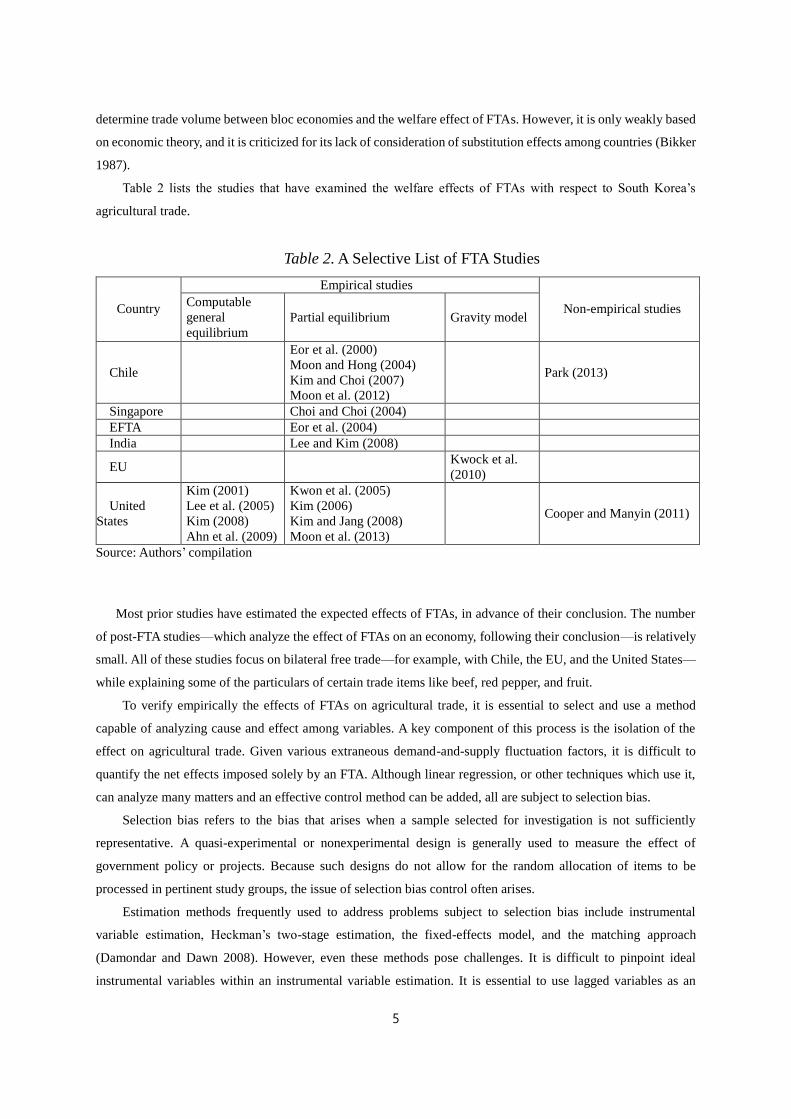
Table 2 lists the studies that have examined the welfare effects of FTAs with respect to South Korea’s
agricultural trade.
Table 2. A Selective List of FTA Studies
Country
Empirical studies
Non-empirical studies Computable
general
equilibrium
Partial equilibrium Gravity model
Chile
Eor et al. (2000)
Moon and Hong (2004)
Kim and Choi (2007)
Moon et al. (2012)
Park (2013)
Singapore Choi and Choi (2004)
EFTA Eor et al. (2004)
India Lee and Kim (2008)
EU Kwock et al.
(2010)
United
States
Kim (2001)
Lee et al. (2005)
Kim (2008)
Ahn et al. (2009)
Kwon et al. (2005)
Kim (2006)
Kim and Jang (2008)
Moon et al. (2013)
Cooper and Manyin (2011)
Source: Authors’ compilation
Most prior studies have estimated the expected effects of FTAs, in advance of their conclusion. The number
of post-FTA studies—which analyze the effect of FTAs on an economy, following their conclusion—is relatively
small. All of these studies focus on bilateral free trade—for example, with Chile, the EU, and the United States—
while explaining some of the particulars of certain trade items like beef, red pepper, and fruit.
To verify empirically the effects of FTAs on agricultural trade, it is essential to select and use a method
capable of analyzing cause and effect among variables. A key component of this process is the isolation of the
effect on agricultural trade. Given various extraneous demand-and-supply fluctuation factors, it is difficult to
quantify the net effects imposed solely by an FTA. Although linear regression, or other techniques which use it,
can analyze many matters and an effective control method can be added, all are subject to selection bias.
Selection bias refers to the bias that arises when a sample selected for investigation is not sufficiently
representative. A quasi-experimental or nonexperimental design is generally used to measure the effect of
government policy or projects. Because such designs do not allow for the random allocation of items to be
processed in pertinent study groups, the issue of selection bias control often arises.
Estimation methods frequently used to address problems subject to selection bias include instrumental
variable estimation, Heckman’s two-stage estimation, the fixed-effects model, and the matching approach
(Damondar and Dawn 2008). However, even these methods pose challenges. It is difficult to pinpoint ideal
instrumental variables within an instrumental variable estimation. It is essential to use lagged variables as an

6
independent variable in the fixed-effects model. In Heckman’s two-stage estimation, it is difficult to determine
ideal explanatory variables that classify the selection equation and the outcome equation (Lee et al. 2008; Kim
2010). The basic logic of the matching approach is to identify what will happen if the object for treatment and
observation is not treated through matching. The matching approach is used to analyze the effect solely of FTAs
among non-FTA countries that have characteristics similar to those of the FTA countries, within a comparison
group. Although it is widely used to analyze the effect of institutions, the matching approach is relatively new to
trade analysis.
Baier and Bergstrand (2009) used the gravity model and Mahalanobis matching to undertake analysis while
focusing on the distance factor. They controlled selection bias through matching, and used the gravity model to
efficiently estimate the effect of FTAs in considering the distance factor. They drew the conclusion that the long-
term effect of FTAs is a stable and significant trade volume increase between signatories. This finding is very
similar to the result obtained through experiments.
Chang and Lee (2011) used pair matching to analyze the effect of trade among General Agreement on Tariffs
and Trade (GATT)/WTO members after signing an FTA. Although they used the same data as Rose (2004), they
reached a different conclusion of a facilitating trade effect following the signing and enforcement of FTAs.
Iacus et al. (2012) used coarsened exact matching (CEM): an effective approach for reducing imbalance
between a treatment group and a comparison group in order to control selection bias. This method, however, leads
to sample loss in the process of coarsening each section of the treatment group and the comparison group.
Therefore, CEM is an approach ideal for a case involving a large sample.
Although they are efficient approaches to estimating the effect of FTAs, Mahalanobis matching, pair
matching, and CEM are not ideal for use in the study of countries with a small number of FTA signatories, like
South Korea. If the number of variables that represent any characteristics is not the same among comparison
groups, problems will occur in selecting sections between groups. In fact, matching based on these variables will
be impossible (Dehejia and Wahba 2002). An alternative used to address this problem is the matching approach
based on propensity scores (i.e., PSM), which has been widely used to analyze the effect of policies. This is a
method used to minimize selection bias, the greatest weakness inherent in a quasi-experimental design. It makes
use of bootstrapping, which allows the treatment group and the comparison group to have as many similar or
identical propensities as possible (Rosenbaum and Rubin 1983).
Hayakawa (2012) used 1:1 nearest-neighbor matching, among other PSM approaches, to determine that FTAs
do not have a great impact on unemployment. Nayga et al. (2011) wanted to identify the effect of school lunch
programs in elementary schools on obesity among school children. This study aimed to control selection bias and
used the nearest-neighbor, kernel, and radius-matching approaches. In particular, the radius-matching approach
was used to widen the scope of radius by 0.5 units on the basis of the treatment group, to compare changes in the
effect of treatment. Kim and Kim (2011) used data matching to analyze wage gaps among temporary workers.
That study identified differences in the wage effect before and after data matching, and robustly explained the
effect of wage gaps by controlling the ratio of the treatment group to the comparison group.
However, only a few studies have used matching approaches to estimate the effects solely of FTAs and no
previous empirical study has examined the effect of FTAs on South Korea’s agricultural trade.
7
III. Empirical Methods and Data
3.1 Selection Bias
It is necessary to compare the conclusion of FTAs in their absence, in order to measure the effect of FTAs on
a country’s agricultural trade. However, in reality, it is impossible to compare cases in which South Korea has
concluded an FTA with one country, to the cases in which has and not concluded that FTA. Therefore, in this study,
PSM analysis is used to identify countries with propensities similar to those of countries who have concluded
FTAs with South Korea as a comparison group. The end point is to analyze outcome differences between the
treatment and comparison groups. This method can have some issues. Selection bias can occur due to unexpected
factors, i.e., effects caused by factors other than FTAs, such as tariffs, natural disasters, social issues, and political
issues. Therefore, in using general linear regression (or methods that apply it), there is a need to use an effective
method to control for these factors.
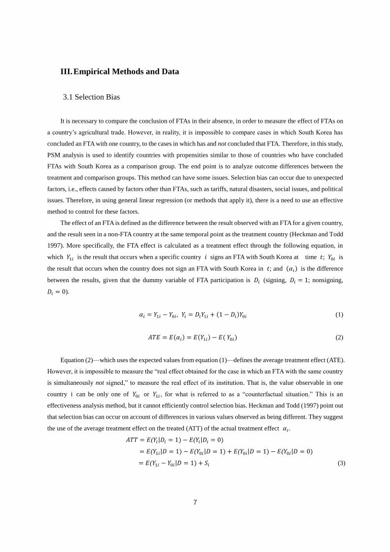
The effect of an FTA is defined as the difference between the result observed with an FTA for a given country,
and the result seen in a non-FTA country at the same temporal point as the treatment country (Heckman and Todd
1997). More specifically, the FTA effect is calculated as a treatment effect through the following equation, in
which 𝑌1𝑖 is the result that occurs when a specific country 𝑖 signs an FTA with South Korea at time 𝑡; 𝑌0𝑖 is
the result that occurs when the country does not sign an FTA with South Korea in 𝑡; and (𝛼𝑖) is the difference
between the results, given that the dummy variable of FTA participation is 𝐷𝑖 (signing, 𝐷𝑖 = 1; nonsigning,
𝐷𝑖 = 0).
𝛼𝑖 = 𝑌1𝑖 − 𝑌0𝑖, 𝑌𝑖 = 𝐷𝑖𝑌1𝑖 + (1 − 𝐷𝑖)𝑌0𝑖 (1)
𝐴𝑇𝐸 = 𝐸(𝛼𝑖) = 𝐸(𝑌1𝑖) − 𝐸( 𝑌0𝑖) (2)
Equation (2)—which uses the expected values from equation (1)—defines the average treatment effect (ATE).
However, it is impossible to measure the “real effect obtained for the case in which an FTA with the same country
is simultaneously not signed,” to measure the real effect of its institution. That is, the value observable in one
country i can be only one of 𝑌0𝑖 or 𝑌1𝑖 , for what is referred to as a “counterfactual situation.” This is an
effectiveness analysis method, but it cannot efficiently control selection bias. Heckman and Todd (1997) point out
that selection bias can occur on account of differences in various values observed as being different. They suggest
the use of the average treatment effect on the treated (ATT) of the actual treatment effect 𝛼𝑖.
𝐴𝑇𝑇 = 𝐸(𝑌𝑖|𝐷𝑖 = 1) − 𝐸(𝑌𝑖|𝐷𝑖 = 0)
= 𝐸(𝑌1𝑖|𝐷 = 1) − 𝐸(𝑌0𝑖|𝐷 = 1) + 𝐸(𝑌0𝑖|𝐷 = 1) − 𝐸(𝑌0𝑖|𝐷 = 0)
= 𝐸(𝑌1𝑖 − 𝑌0𝑖|𝐷 = 1) + 𝑆𝑖 (3)
8
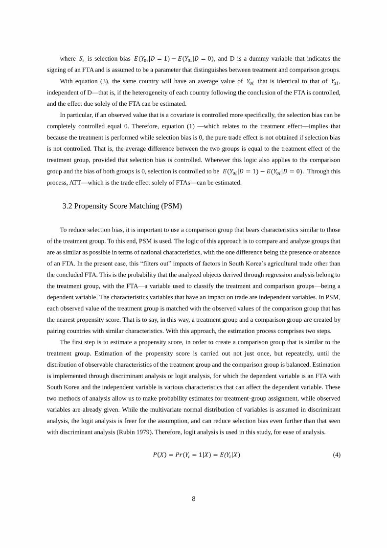
where 𝑆𝑖 is selection bias 𝐸(𝑌0𝑖|𝐷 = 1) − 𝐸(𝑌0𝑖|𝐷 = 0), and D is a dummy variable that indicates the
signing of an FTA and is assumed to be a parameter that distinguishes between treatment and comparison groups.
With equation (3), the same country will have an average value of 𝑌0𝑖 that is identical to that of 𝑌1𝑖 ,
independent of D—that is, if the heterogeneity of each country following the conclusion of the FTA is controlled,
and the effect due solely of the FTA can be estimated.
In particular, if an observed value that is a covariate is controlled more specifically, the selection bias can be
completely controlled equal 0. Therefore, equation (1) —which relates to the treatment effect—implies that
because the treatment is performed while selection bias is 0, the pure trade effect is not obtained if selection bias
is not controlled. That is, the average difference between the two groups is equal to the treatment effect of the
treatment group, provided that selection bias is controlled. Wherever this logic also applies to the comparison
group and the bias of both groups is 0, selection is controlled to be 𝐸(𝑌0𝑖|𝐷 = 1) − 𝐸(𝑌0𝑖|𝐷 = 0). Through this
process, ATT—which is the trade effect solely of FTAs—can be estimated.
3.2 Propensity Score Matching (PSM)
To reduce selection bias, it is important to use a comparison group that bears characteristics similar to those
of the treatment group. To this end, PSM is used. The logic of this approach is to compare and analyze groups that
are as similar as possible in terms of national characteristics, with the one difference being the presence or absence
of an FTA. In the present case, this “filters out” impacts of factors in South Korea’s agricultural trade other than
the concluded FTA. This is the probability that the analyzed objects derived through regression analysis belong to
the treatment group, with the FTA—a variable used to classify the treatment and comparison groups—being a
dependent variable. The characteristics variables that have an impact on trade are independent variables. In PSM,
each observed value of the treatment group is matched with the observed values of the comparison group that has
the nearest propensity score. That is to say, in this way, a treatment group and a comparison group are created by
pairing countries with similar characteristics. With this approach, the estimation process comprises two steps.
The first step is to estimate a propensity score, in order to create a comparison group that is similar to the
treatment group. Estimation of the propensity score is carried out not just once, but repeatedly, until the
distribution of observable characteristics of the treatment group and the comparison group is balanced. Estimation
is implemented through discriminant analysis or logit analysis, for which the dependent variable is an FTA with
South Korea and the independent variable is various characteristics that can affect the dependent variable. These
two methods of analysis allow us to make probability estimates for treatment-group assignment, while observed
variables are already given. While the multivariate normal distribution of variables is assumed in discriminant
analysis, the logit analysis is freer for the assumption, and can reduce selection bias even further than that seen
with discriminant analysis (Rubin 1979). Therefore, logit analysis is used in this study, for ease of analysis.
𝑃(𝑋) = 𝑃𝑟 (𝑌𝑖 = 1|𝑋) = 𝐸(𝑌𝑖|𝑋) (4)

9
In equation (4), X is each feature vector of FTA countries and non-FTA countries, and 𝑃(𝑋) is the
probability of signing an FTA under the condition of such features. The key assumptions of the propensity scores
are described below.
(𝑌0𝑖,𝑌1𝑖) ⊥ 𝐷𝑖|𝑋 (5)
0 < 𝑃𝑟(𝐷𝑖 = 1|𝑋) < 1 (6)
Equation (5) is about the conditional independent assumption (CIA), which means that, while the observed
feature (𝑋) is given in the most important process used to justify matching, the concluded FTA (𝐷) of a country
is independent of the potential outcome (𝑌0𝑖,𝑌1𝑖) of the FTA. This means that any feature not observed by
controlling all differences that influence the effect of a concluded FTA does not have an impact on the effect—
that is, 𝐸(𝑌1𝑖|𝐷𝑖 = 1) − 𝐸(𝑌0𝑖|𝐷𝑖 = 0). Equation (6), on the other hand, is about the common support assumption.
In this equation, 𝑃(𝑋) is a continuous variable between 0 and 1, and there is the assumption that the probability
distributions of countries who have signed an FTA (i.e., an FTA country) with South Korea and non-FTA countries
overlap within the same range (Rosenbaum and Rubin 1983). A strongly ignorable treatment assumption between
variables established on the assumptions of equations (5) and (6) contributes to the strongly ignorable assumption
vis-à-vis the propensity score, which is a probability function. The issue of dimensions that occur in matching
based on variables can be addressed by comparing differences by virtue of propensity scores, which summarize
the characteristics of variables as one figure.
The second step is to find a non-FTA country group with propensity scores similar to those of the FTA country
group, for ATT values that cannot be estimated merely by estimating propensity scores in the first step; this is
done to analyze the effect of FTAs by matching differences. That is to say, the observable characteristics of the
two groups will have the same distribution, so that the effect in the absence of selection bias can be estimated.
In this case, we can select various matching approaches, and a selection can be made through stratification
matching, kernel matching, and nearest-neighbor matching to determine matching between FTA countries with
South Korea and non-FTA countries (Heckman and Todd 1997).
Stratification matching uses a process of dividing the scope of changing propensity scores into subgroups,
and classifying each subgroup with both treatment and the FTA group as units with similar propensities. This is
done to obtain weighted averages of the effect calculated for each group. The kernel-matching approach uses a
process that leverages the kernel function to give higher weights to all members of the non-FTA group nearer to
the propensity score of the FTA group, and smaller weights to the members farther from the propensity score. The
nearest-neighbor-matching approach sorts two groups of FTA countries and non-FTA countries in random order
to find and match members of the non-FTA country group with a propensity score nearest to that of the members
of the FTA country group, in a 1:1 manner. This approach repeats the aforementioned matching process for all
countries to calculate the difference between FTA countries and non-FTA countries, to reduce selection bias and
thus obtain robust results. However, because with the nearest-neighbor-matching approach the scope of the
common area in estimating the propensity score is narrow, the size of the matching sample is relatively small.

10
In conclusion, the PSM approach holds the same basic framework regarding differences between the
treatment and comparison groups, but its results can differ from those of stratification matching, nearest-neighbor
matching, kernel matching, depending on the given weights, the definition of the number of sections, the standards
of the treatment group and the comparison group, and the definition of “function values.” The aforementioned
matching approaches can be seen to offset each other in terms of bias and variance, if they are evaluated on those
bases. This means there is no absolutely superior matching approach, which makes it necessary to compare
estimation results from a variety of matching approaches (Becker and Ichino 2002; Caliendo and Kopeining 2008;
Kim 2010).
3.3 Data
Table 3 lists variable definitions and data sources.
Table 3. Data Sources
Variable Unit Source
FTAs Dummy WTO
Trade value USD Global Trade Atlas
GDP per capita USD World Bank Development Indicators
Total population Person World Bank Development Indicators
Distance weighed Km Centre d’É tudes Prospectives et d’Informations Internationales.
Trade balance USD Global Trade Atlas
With PSM, there is a cause-and-effect relationship between the FTA country group that contains South Korea
and the non-FTA country group. Accurate ATT values can be estimated by using variables that satisfy the
assumption of conditional independence and are balanced in the common area. Therefore, in this study, we
pinpoint a variable that is balanced between the conclusion of an FTA or non-FTA, and which satisfies the
assumption of conditional independence and is within the common area (Baier and Bergstrand 2009). The
variables are the volume of agricultural trade between the two countries, GDP per capita, population, distance,
and balance of trade.
The volume of agricultural trade and the balance of trade between two countries is sourced from the Global
Trade Atlas. The agricultural products to be analyzed are based on the HS codes 01–24. GDP per capita and
population data are sourced from World Bank Development Indicators (WDI). The latest WDI data are from 2012,
and the information within the data analyzed in this study is also from 2012. Data regarding the distance variable
are sourced from the indicators of the Centre d’É tudes Prospectives et d’Informations Internationales (CEPII), a
French research institute.
As of 2012, South Korea had signed 15 FTAs. The relatively small number of FTAs that South Korea had
signed between 2004 and 2006 is not sufficiently large to create a treatment group. Therefore, cross-sectional data
from 2012 are used in the analysis in this study.
Table 4 provides summary statistics of data.

11
Table 4. Summary Statistics of Data
Variable Obs. Mean Std. Err. Min Max
Import
FTAs 204 0.215686 0.412309 0 1
Trade value 204 1.25E+08 5.37E+08 0 5.87E+09
GDP per capita 184 14479.47 20444.74 251.0145 103858.9
Total population 204 3.57E+07 1.34E+08 9860 1.35E+09
GDP per capita of
South Korea 204 24453.97 0 24453.97 24453.97
Total population
of South Korea 204 5.00E+07 0 5.00E+07 5.00E+07
Distance weighed 204 9484.03 3744.478 354.549 19563.9
Trade balance 204 –4.60E+08 5.28E+09 –7.52E+10 1.89E+09
Export
FTAs 195 0.2205128 0.41566 0 1
Trade value 195 3.54E+07 1.90E+08 0 2.30E+09
GDP per capita 179 14467.2 20483.53 266.589 103858.9
Total population 195 3.55E+07 1.35E+08 9860 1.35E+09
Distance weighed 195 9541.234 3734.13 951.737 19563.9
Trade balance 193 –4.86E+08 5.43E+09 –7.52E+10 1.89E+09
Because there are cases of no imports or small import volumes within the analysis period of 2012, the use of
ordinary least squares is very likely to cause bias. The PSM approach is used to control this selection bias. The
statistics program used to undertake empirical analysis is Stata 12.
South Korea imports agricultural products from 204 countries, and it exports to 195 countries. As of 2010,
South Korea had signed FTAs with about 7% of these countries. The country signed FTAs with the EU and the
United States, two large economic entities, as of 2012, when those numbers became 21% and 22%, respectively.2)
IV. Estimation Results and Discussion
4.1 Propensity Scores
Logit analysis is used to estimate the propensity score, depending on the effect of FTAs. The estimated
parameters of logit analysis are used to calculate the propensity score, and to investigate the satisfaction of both
the CIA—the major premise of PSM estimation—and the common support assumption. Tables 6 illustrates the
results of logit analysis for each country of export or import of South Korea’s agricultural products, to identify
those factors that have had an impact on the signing of FTAs. These results were obtained by using 2012 data.3)
2) The summary statistics of the 2010 data are provided in the Appendix.
3) The 2010 data by logit analysis are not any different from the results from the 2012 data; these are provided in the Appendix.

12
In Table 5, one can see similar aspects of coefficient signs that illustrate the cases of the importation and
exportation of South Korea’s agricultural products. The estimation results illustrate that a country is more likely
to conclude an FTA with South Korea if its GDP is greater, its population is larger, it is located geographically
near to South Korea, and has a comparatively larger trade balance. The larger estimates of coefficient values
among significant variables were of GDP, for both imports and exports. This implies that national competitiveness
is an important factor in signing an FTA.
Table 5. Logit Estimation Results
Explanatory variable Dependent variable
Import Export
GDP per capita of importers 0.0000375***
(0.00000917)
0.0000388***
(9.46E-06)
Total population 0.000000000837**
(1.13E-09)
0.00000000105**
(1.17E-09)
Distance weighed –0.0001457*
(0.0000605)
–0.0001434*
(0.000061)
Trade balance 0.00000000000723*
(5.79E-11)
0.00000000000953*
(6.13E-11)
Constant –0.6095753
(0.5960046)
–0.6133886
(0.6052889)
Log-likelihood value –82.490227 –80.840728
Prob > 𝑋2 0.0000 0.0000
Pseudo 𝑅2 0.1654 0.1711
Note: *, **, *** denote significance at the 10%, 5%, and 1% levels, respectively
Table 6 shows the common area result in the process of estimating propensity scores. The sample size was
reduced when considering the characteristics of the covariates in calculating the propensity scores. Between 1%
and 99%, in 2010, the common area was between 0.002 and 0.362 (where South Korea imports agricultural
products) and between 0.002 and 0.366 (where South Korea exports them). In 2012, those ranges were 0.061–
0.923 and 0.064–0.932, respectively.
Figure 2 shows the propensity scores in the common area. The satisfaction of the common area is greater
between the treatment group and the comparison group, as the two bars are similar in height.
The comparison group with a propensity score similar to that of the treatment group is subdivided into several
blocks in terms of percentiles, to determine the satisfaction of conditional independence. The subdivided blocks
include four countries for each of imports and exports in 2010, and five countries for each of imports and exports
in 2012. This grouping allows one to see differences in average propensity score between the two groups. As a
result of analysis, no difference is found between FTA and non-FTA countries, and this implies the satisfaction of
the assumption of conditional independence (Kim et al. 2013).4)
4) With PSM undertaken through Stata, the program calculates conditional independence. If this assumption is violated,
matching is not implemented. We omit from this study the Stata-based process of examining conditional independence.

13
Table 6. Common Support
Year Sample Propensity score Common support
Before After Minimum Maximum
2010 Import 15 14 0.002 0.362
Export 15 14 0.002 0.366
2012 Import 44 42 0.061 0.923
Export 43 42 0.064 0.932
Figure 2. Propensity Scores (Frequencies of Probability Intervals by Treatments and Models)
4.2 Stratification, Kernel, and Nearest-Neighbor Matching
The stratification-matching, kernel-matching, and nearest-neighbor-matching approaches are used to
investigate the effect of FTAs on South Korea’s agricultural trade. The nearest-neighbor-matching approach,
which leverages 1:1 matching, is generally used. The one divided group has four countries for each of imports
and exports in 2010; the other divided group contains five countries for each of imports and exports in 2012. Here,
the number of countries in each group is the same as those in the groups calculated through the common area and
used in tandem with the stratification-matching approach. Kernel matching5) uses the Epanechnikov kernel
5) In kernel matching, matching is implemented with a plurality of treatment groups per comparison group sample. In this case,
greater weight is given to a treatment group sample for which the propensity score is nearer to that of the comparison group.
The Gaussian kernel, Epanechnikov kernel, or Unimodal kernel is used, depending on the assumption that the weight
follows a certain distribution function. The Epanechnikov kernel is used in this study to analyze matching.

14
function, and for the purpose of analysis, each bandwidth is 0.05. The trust region of the FTA effect is estimated
through bootstrapping. Resampling through bootstrapping is repeated 1,000 times. This applies to all matching
analyses. It is possible to identify reductions in selection bias by comparing the figures before and after each
matching for which bootstrapping was carried out. Table 7 illustrates changes in selection bias for each matching
type.
Table 7. Bias Reduction after Matching
Year Sample Matching method Bias reduction (%, after matching)
2010
Importers
Stratification matching –31.7(%)
Kernel matching –29.6(%)
Nearest-neighbor matching –38.9(%)
Exporters
Stratification matching –32.5(%)
Kernel matching –30.3(%)
Nearest-neighbor matching –40.1(%)
2012
Importers
Stratification matching –31.3(%)
Kernel matching –28.9(%)
Nearest-neighbor matching –39.6(%)
Exporters
Stratification matching –33.7(%)
Kernel matching –31.6(%)
Nearest-neighbor matching –41.1(%)
Matching can lead to effective or ineffective estimations, depending on how much heterogeneity is controlled
between the variables of the two comparison groups—that is, the degree to which bias reduction contributes to
measurements of the true effect of FTAs. The estimation results reveal that each group is balanced with respect to
the average of each variable after matching, compared to the average of each variable prior to matching. Bias is
reduced with each matching approach, and each instance of bias reduction is different, depending on the matching
type. Nearest-neighbor matching reduced bias the most, followed by stratification matching and kernel matching.
Therefore, it is concluded that nearest-neighbor matching is the best approach for controlling heterogeneity
between the treatment and comparison groups.
Table 8 illustrates South Korea’s net agricultural trade after signing FTAs in 2010. South Korea concluded
FTAs with five trade countries (i.e., Chile, Singapore, EFTA, ASEAN, and India) in 2010, and with 16 countries
in total. However, from these samples for matching, 14 FTA countries for both imports and exports, as well as 9–
152 and 9–157 non-FTA countries for imports and exports, respectively, were used to study matching. South Korea
is a net importer of agricultural products. Its agricultural product exports account for a relatively small proportion
of overall trade, in comparison to its imports. Nonetheless, all were found to have positive signs (+) in all matching
approaches. Therefore, we can conclude that FTAs signed in 2010 contributed to increases in both imports and
exports.

15
Table 8. Agricultural Trade Effects of FTAs in 2010
Matching method Treatment group
(FTA countries)
Control group
(non-FTA countries) ATT
Import
Stratification matching 14 165 198**
(7.67e+07)
Kernel matching 14 165 176**
(5.35e+07)
Nearest-neighbor
matching 14 11
113***
(1.86e+08)
Export
Stratification matching 14 158 40.3*
(2.02e+07)
Kernel matching 14 158 40.4*
(2.10e+07)
Nearest-neighbor
matching 14 9
40.0**
(1.70e+07)
Note: *, **, and *** denote significance at the 10%, 5%, and 1% levels, respectively.
Table 9 shows agricultural trade effects of FTAs in 2012. South Korea signed FTAs with the EU and Peru in
2011, and the United States in 2012, to bring the total number of FTA countries to 44. This implies an increase of
28 FTA countries compared to 2010. Forty-two countries were used in the estimations, and the treatment group
was reduced by two when calculating the common area prior to matching. It is thought that the reduction occurred
in the process of calculating the countries whose propensity scores were similar to those of the countries in the
comparison group. In particular, nearest-neighbor matching shows an obvious reduction in the sample within the
comparison group. This result derives from the narrower scope of the common area in estimating the propensity
score. As such, the reduced sample in the comparison group is advantageous, in that the heterogeneity with the
treatment group is controlled best, and is therefore most effective in controlling selection bias and calculating
relatively robust estimation results.
In comparison to estimations that derive from each matching approach for differences between 2010 and
2012, stratification matching reveals an increase from USD198 million to USD206 million. Kernel matching and
nearest-neighbor matching, meanwhile, reveals an increase from USD176 million to USD185 million, and from
USD113 million to USD156 million, respectively. With respect to exports, all matching approaches reveal
increases in 2012, relative to 2010. Stratification matching reveals an increase from USD40.3 million to USD57.2
million; kernel matching, from USD40.4 million to USD67.4 million; and nearest-neighbor matching, from
USD40 million to USD47.7 million. The FTA trade effect illustrated in Tables 8 and 9 shows slight differences,
depending on the matching approach used. However, all result figures carry a positive sign (+), and this implies
that FTAs have had the effect of increasing South Korea’s net agricultural trade.

16
Table 9. Agricultural Trade Effects of FTAs in 2012
Matching method Treatment group
(FTA countries)
Control group
(non-FTA countries) ATT
Import
Stratification matching 42 137 206**
(1.50e+08)
Kernel matching 42 137 185**
(1.44e+08)
Nearest-neighbor matching 42 23 156***
(1.14e+08)
Export
Stratification matching 42 132 57.2**
(4.05e+07)
Kernel matching 42 132 67.4*
(5.31e+07)
Nearest-neighbor matching 42 20 47.7**
(5.93e+07)
Note: *, **, and *** denote significance at the 10%, 5%, and 1% levels, respectively.
A comparison of ATT values in terms of matching approaches shows that with respect to imports in 2010
and 2012, stratification matching is superior to kernel matching, which is in turn superior to nearest-neighbor
matching. For exports, kernel matching is superior to stratification matching, which is in turn superior to nearest-
neighbor matching. This is because while bias can increase, kernel matching can reduce the standard deviation by
using all the variables within a controlled group. Nearest-neighbor matching has an ATT difference, because
events likely to occur by virtue of the connected variables nearest to the propensity score are omitted, or because
of the large standard deviation that occurs and is attributable to the PSM of other variables (Kim et al. 2013)
Table 10 compares ATE and ATT values generated through matching. This allows us to investigate
differences between the selection bias effect controlled through various matching approaches and the uncontrolled
effect. In 2010, the ATE for agricultural products between FTA countries and non-FTA countries was USD852
million for imports and USD184 million for exports. In 2012, on the other hand, the ATE for agricultural products
was USD314 million for imports and USD78 million for exports. The ATE values in 2012 were smaller than those
in 2010, and this implies an increased trade volume with FTA countries that in turn reduces exports to non-FTA
countries. However, with respect to analysis of the results obtained through the ATE, the results estimated by
excluding selection bias do not constitute a pure FTA effect.
Table 10. Comparisons of ATE and ATT (millions of US dollars)
Sample Import Export
2010 2012 2010 2012
ATE 852 314 184 78
ATT
Stratification matching 198 206 40.3 57.2
Kernel matching 176 185 40.4 67.4
Nearest-neighbor matching 113 156 40.0 47.7
On the other hand, the ATT—for which selection bias is controlled through PSM—reveals a difference of
USD156–206 million for when selection bias was controlled. This implies a relatively accurate FTA effect in

17
comparison to that derived with the ATE. All ATT figures are smaller than the ATE figures; therefore, bias control
was a clearly factor that led to the difference between the estimated ATE and ATT figures. More significantly, this
means that previous studies on the trade effect of signed FTAs have overestimated the effect, as they do not address
selection bias.
In summary, FTAs have contributed to increases in both imports and exports agricultural products in South
Korea. Because their effect on imports is greater than that on exports, there are concerns about their impact on the
overall domestic agricultural industry. However, analysis of ATE prior to matching, as well as of ATT—which
involves the result of each matching approach—reveals that the effect solely of FTAs is smaller than all ATE
figures. This implies that the impact of FTAs on South Korea’s agricultural trade is not overly significant.
V. Conclusions
This study used PSM to control selection bias, to investigate the effect solely of FTAs on South Korea’s
agricultural trade. It also sought to analyze the effect of FTAs on international trade. Differences in treatment
effects with regard to 2010 and 2012 data were compared and analyzed to obtain robust results.
Analysis of the effect of FTAs on South Korea’s agricultural trade revealed increased imports of USD8
million when using stratification matching, USD9 million when using kernel matching, and USD43 million when
using nearest-neighbor matching. With respect to exports, the increases were USD16.9 million with stratification
matching, USD27 million with kernel matching, and USD7.7 million with nearest-neighbor matching. Clearly,
the FTA trade effect varied slightly, depending on the matching approach used. However, all results bore a positive
effect (+), and this implies that FTAs contribute to an increased net trade in South Korea’s agricultural products.
ATT was compared to ATE to exam differences between selection bias controlled through the use of various
matching approaches and selection bias left uncontrolled. The result is that the ATE figures—which constitute the
average treatment effect for which bias was not controlled—are greater than the ATT estimates calculated through
matching. This suggests that differences between ATE and ATT estimates depend on whether or not selection bias
was controlled. Most prior studies on the effect of FTAs on trade have not addressed the issue of selection bias
and thus have overestimates their effect.
This study identifies the smaller impact of controlled selection bias on South Korea’s agricultural product
market, relative to uncontrolled selection bias. However, it seems that South Korea, a net importer of agricultural
products, will import more agricultural products than it will export, after signing FTAs. In this way, FTAs will
continue to make South Korea’s domestic agricultural industry be vulnerable to import competition, which sheds
light on policy reactions, including income safety net measures and trade adjustment assistance.
The data used in this study are not complete and should be supplemented with future research. An FTA does
not cover all items subject to FTA tariffs. Although a certain imported item can be included in a concession list,
not all items on that list are subject to lowered tariffs the moment an FTA is signed. Rather, products are subject
to various tariff exemption rates and a schedule, depending on the items traded by the counterpart FTA countries.
Therefore, future panel analysis that combines cross-sectional analysis to examine the long-term trade structure—
especially that featuring vertical analysis, by extending the observation period—will help derive more significant
results.

18
References
Ahn, D. H., J. B. Lim., and A. S. Choi (2009). Analysis of inter-industrial effects resulting from the impacts of
the Korea-US FTA on Korean agricultural sector, Journal of Rural Development. 32(5): 83-108. (in Korean)
http://www.krei.re.kr/web/www/15?p_p_id=EXT_BBS&p_p_lifecycle=0&p_p_state=normal&p_p_mode
=view&_EXT_BBS_struts_action=%2Fext%2Fbbs%2Fview_message&_EXT_BBS_messageId=10037
Baier, S. L., and J. H. Bergstrand (2009). Estimating the effects of free trade agreements on international trade
flows using matching econometrics, Journal of International Economics, 77(1): 63-76.
https://ideas.repec.org/a/eee/inecon/v77y2009i1p63-76.html
Becker, S.O., and A. Ichino (2002). Estimation of Average Treatment Effects based on Propensity Scores, The
STATA Journal. 2(4): 358-377. http://www.stata-journal.com/article.html?article=st0026
Bikker, J. A. (1987). An International Trade Flow Model with Substitution: An Extension of the Gravity Model,
Journal of Comparative Economics. 40(3): 315-337. https://ideas.repec.org/a/bla/kyklos/v40y1987i3p315-
37.html
Blundell, R., and M. Costa-Dias (2009). Alternative Approaches to Evaluation in Empirical Microeconomics,
Journal of Human Resources, 44(3): 565-640. https://ideas.repec.org/p/iza/izadps/dp3800.html
Caliendo, M., and S. Kopeining (2008). Some practical guidance for the implementation of propensity score
matching, Journal of Economic Surveys. 22(1): 31-72.
http://www.iza.org/en/webcontent/publications/papers/viewAbstract?dp_id=1588
Chang, P.L., and M.J. Lee (2011). The WTO trade effect. Journal of International Economics 85(1): 53–71.
https://ideas.repec.org/a/eee/inecon/v85y2011i1p53-71.html
Choi, S. I. and H. B. Choi (2004). Economic Effects of Korea-Singapore Free Trade Agreement on the Fisheries
Sector, The Journal of Fisheries Business Administration. 35(2): 71-90. (in Korean)
http://www.riss.kr/search/detail/DetailView.do?p_mat_type=1a0202e37d52c72d&control_no=7c019c415a
0d8ff2ffe0bdc3ef48d419
Cooper, W., and M. Manyin (2011). (The)U.S.-South Korea free trade agreement(KORUS FTA): looking ahead-
-prospects and potential challenges, International Journal of Korean Studies, 15(2): 127-150.
http://connection.ebscohost.com/c/articles/71993889/u-s-south-korea-free-trade-agreement-korus-fta-
looking-ahead-prospects-potential-challenges
Damondar, N.G., and C.P. Dawn (2008) Basic Econometrics, 5th Edition. The McGraw-Hill Companies, Inc.,
New York; ISBN 978-0-07-337577-9.
Dehejia, R., and S. Wahba (2002). Propensity score-matching methods for non-experimental causal studies,
Review of Economics and Statistics, 84(1): 151-161. https://ideas.repec.org/a/tpr/restat/v84y2002i1p151-
161.html
Eor, M. K., J. O. Lee., Y. G. Choi., T. G. Kim., and J. G. Jung (2000). Competitive Advantage of Chilean Fruit
Industry and Trade Outlook. Korean Journal of Agricultural Management and Policy, 27(2): 132-146. (in
Korean)
http://www.riss.kr/search/detail/DetailView.do?p_mat_type=1a0202e37d52c72d&control_no=0bdd1ac1e1ac1716
19
Eor, M. K., O. B. Kwon., and H. J. Lee (2004). Effects of FTA between Korea and EFTA on Agricultural Sector,
Korea Rural Economic Institute (KREI) Research Working Paper, Seoul. (in Korean)
http://www.krei.re.kr/web/www/23?p_p_id=EXT_BBS&p_p_lifecycle=0&p_p_state=normal&p_p_mode
=view&_EXT_BBS_struts_action=%2Fext%2Fbbs%2Fview_message&_EXT_BBS_messageId=1955
Frankel, J., D. Romer., and T. Cyrus (1996). Trade and growth in East Asian countries: cause and effect? National
Bureau of Economic Research Working Paper. No. 5732, Cambridge. http://www.nber.org/papers/w5732
Hayakawa K. (2012). Impacts of FTA utilization on firm performance. IDE Discussion Papers, Institute of
Developing Economies. Japan External Trade Organization(JETRO).
https://ideas.repec.org/p/jet/dpaper/dpaper366.html
Heckman, J.J., and Petra E. Todd (1997). Matching as an Econometric Evaluation Estimator: Evidence from
Evaluating a Job Training Programme, Review of Economic Studies, 64(4): 605-654.
https://ideas.repec.org/a/bla/restud/v64y1997i4p605-54.html
Iacus, S., G. King, and G. Porro (2012). Multivariate Matching Methods That Are Monotonic Imbalance Bounding,
Journal of the American Statistical Association, 106(493): 345-346. http://gking.harvard.edu/files/abs/cem-
math-abs.shtml
Kawai M., and G. Wignaraja (2014). Trade policy and growth in Asia, Asian Development Bank Institute Working
Paper, No. 495, Tokyo. http://www.adbi.org/working-paper/2014/08/15/6375.trade.policy.growth.asia/
Kim, C.S. (2001). The economic effects of the Korea–Chile Free Trade Agreement using the CGE Model, Korean
Journal of Agricultural Management and Policy, 28(3): 438–456. (in Korean)
http://www.riss.kr/search/detail/DetailView.do?p_mat_type=1a0202e37d52c72d&control_no=3a6513b06e29a835
Kim, C.S. (2008). The economic effects of the Korea–EU FTA under the Korea–USA FTA using CGE, Journal
of International Economics, 14(1): 137–162. (in Korean)
http://www.riss.kr/search/detail/DetailView.do?p_mat_type=1a0202e37d52c72d&control_no=976f36b707
b766ecffe0bdc3ef48d419
Kim, S.A., and J.Y. Kim (2011). Wage differentials between regular and irregular workers, Korean Journal of
Labor Economics, 34(2): 53–78. (in Korean)
http://www.riss.kr/search/detail/DetailView.do?p_mat_type=1a0202e37d52c72d&control_no=a5df90e948
61ded8ffe0bdc3ef48d419
Kim, S.H., and D.H. Jang (2008). Measuring the impact of Korea–U.S. FTA on the Korean dairy market: focusing
on cheese and butter markets, Journal of Rural Development, 31(4): 151–167. (in Korean)
http://www.riss.kr/search/detail/DetailView.do?p_mat_type=1a0202e37d52c72d&control_no=e20c2f83f6
b2b1a0ffe0bdc3ef48d419
Kim, S.Y. (2010). The evaluation of food labeling effect using the matching method, Journal of Rural
Development, 51(3): 47–71. (in Korean)
http://www.riss.kr/search/detail/DetailView.do?p_mat_type=1a0202e37d52c72d&control_no=7b529f323d
89793effe0bdc3ef48d419

20
Kim, T.Y., D.B. Han., J.H. Ann., and S.H. Lee (2013). Effect of mothers’ identification of nutrition labeling on
children’s obesity, Korean Journal of Health Economics and Policy, 19(3): 51–82. (in Korean)
http://www.riss.kr/search/detail/DetailView.do?p_mat_type=1a0202e37d52c72d&control_no=a4a41e77d2
d207c6ffe0bdc3ef48d419
Kim, Y.S. (2006). Measuring an FTA Impact in a Partial Equilibrium Model Considering Substitution Effects:
Application to Korea Beef Industry, Journal of Rural Development, 47(3): 31–51. (in Korean)
http://www.riss.kr/search/detail/DetailView.do?p_mat_type=1a0202e37d52c72d&control_no=1a4a84744f
3b79a0
Kim, Y.S., and S.K. Choi (2007). Ex post evaluation of the Korea–Chile FTA in terms of demand side: application
to Chilean grapes, Journal of Rural Development, 48(1): 81–98. (in Korean)
http://www.riss.kr/search/detail/DetailView.do?p_mat_type=1a0202e37d52c72d&control_no=165de4c7ca
5ec8a2
Kwock, C. K., J. K. Jang., and H. J. Kim (2010). Effects of Korea·EU Free Trade Agreement in Agro-food Sector:
A Gravity Model Approach, Journal of Rural Development, 51(1): 1-18. (in Korean)
http://www.riss.kr/search/detail/DetailView.do?p_mat_type=1a0202e37d52c72d&control_no=a4616126da
86c134ffe0bdc3ef48d419
Kwon, O. B., S. K. Choi., J. H. Song, B. S. Kim., S. J. Hong., K. P. Kim., H. J. Kang., and J. N. Heo (2005).
Strategies for Agricultural Sector To Cope With Free Trade Agreements, Korea Rural Economic Institute
(KREI) Research Working Paper, Seoul. (in Korean)
http://www.riss.kr/search/detail/DetailView.do?p_mat_type=d7345961987b50bf&control_no=882a9d872e
64f5a9ffe0bdc3ef48d419
Lee, C.S., J.H, Park., and O.B. Kwon (2005). Economic Effects of a Korea–U.S. FTA on the Korean Agricultural
Sector, Korea Rural Economic Institute (KREI) Research Working Paper, Seoul. (in Korean)
http://www.riss.kr/search/detail/DetailView.do?p_mat_type=d7345961987b50bf&control_no=21a9eb258a
680a9bffe0bdc3ef48d419
Lee, J.H., and K.Y. Kim (2008). A study on the criteria for determining the country of origin in the FTA between
India and Korea, Journal of Korea Trade, 33(3): 159–184. (in Korean)
http://www.riss.kr/search/detail/DetailView.do?p_mat_type=1a0202e37d52c72d&control_no=08f1f61843
dad8d4ffe0bdc3ef48d419
Lee, S.W., J.G. Kim., Y.B. Lee, K.H. Jang., and M.H. Lee (2008). Program evaluation and selection bias: the
sequential selection model for the government loan program for small business, Korean Public
Administration Quarterly, 42(1): 197–227. (in Korean)
http://www.riss.kr/search/detail/DetailView.do?p_mat_type=1a0202e37d52c72d&control_no=dbaecd8f9c
7764c6ffe0bdc3ef48d419
Moon, C.G., and J.H. Hong (2004). Monetary loss estimates of the domestic fruit industry with the effectuation
of the Korea–Chile FTA, Korea Review of Applied Economics, 6(1): 5–48. (in Korean)
http://www.riss.kr/search/detail/DetailView.do?p_mat_type=1a0202e37d52c72d&control_no=2075d16131
34494dffe0bdc3ef48d419

21
Moon, H.P., M.K. Eor., H.U. Park., S.H. Oh., I.S. Jeon., and S.G. Jeon (2012). Strategy in Response to the Free
Trade Agreement (FTA) in the Agricultural Sector: An Economic Effect Analysis of Domestic Measures
Related to the Korea–Chile FTA, Korea Rural Economic Institute (KREI) Research Working Paper, Seoul.
(in Korean)
http://www.riss.kr/search/detail/DetailView.do?p_mat_type=d7345961987b50bf&control_no=6d5fde11b3
70896fffe0bdc3ef48d419
Moon, H.P., H.K. Lee., and H.U. Park (2013). Impacts of the KORUS FTA’s orange import tariff-cut on domestic
fruit prices, Journal of Rural Development, 54(1): 15–38. (in Korean)
http://www.riss.kr/search/detail/DetailView.do?p_mat_type=1a0202e37d52c72d&control_no=7284aa7993
2ba973ffe0bdc3ef48d419
Nayga, R.M., B.L. Campbell., and J.L. Park (2011). Does the national school lunch program improve children’s
dietary outcome? American Journal of Agricultural Economics, 93(4): 1099–1130.
https://ideas.repec.org/a/oup/ajagec/v93y2011i4p1099-1130.html
Palley, T.I. (2012). The rise and fall of export-led growth, Investigación Económica, LXXI280, pp. 141-161.
http://www.levyinstitute.org/publications/the-rise-and-fall-of-export-led-growth
Park, H.H. (2013). Analysis on Agricultural Trade Effects of FTA and Implications –Focusing on Korea-Chile
FTA. Journal of Korea Trade 38(2): 159-178. (in Korea)
http://www.riss.kr/search/detail/DetailView.do?p_mat_type=1a0202e37d52c72d&control_no=cdf9a1a73c
ce24bcffe0bdc3ef48d419
Rose, A.K. (2004). Do we really know that the WTO increases trade? American Economic Review 94(1): 98–
144. https://ideas.repec.org/a/aea/aecrev/v94y2004i1p98-114.html
Rosenbaum, P.R., and D.B. Rubin (1983). The central role of the propensity score in observational studies for
causal effects. Biometrika Trust 70: 41–55. http://biomet.oxfordjournals.org/content/70/1/41
Rubin, D.B. (1979). Using multivariate matched sampling and regression adjustment to control bias in
observational studies. Journal of the American Statistical Association 40: 318–328.
http://www.jstor.org/discover/10.2307/2286330?sid=21106288960843&uid=3738392&uid=2134&uid=2&
uid=4&uid=70

22
Appendix 1. Descriptive Statistics of Dependent Variable (2010)
Variance Obs. Mean Standard error Minimum Maximum
Imports
FTAs 204 0.078431 0.269511 0 1
Trade value 204 9.63E+07 4.64E+08 0 5.33E+09
GDP per capita 184 13801.99 20764.8 219.5298 145229.8
Total population 204 3.49E+07 1.32E+08 9827 1.34E+09
GDP per capita of
South Korea 204 22151.21 0 22151.21 22151.21
Total population of South Korea
204 4.94E+07 0 4.94E+07 4.94E+07
Distance weighed 204 9484.03 3744.478 354.549 19563.9
Trade balance 204 –6.94E+08 8.91E+09 –1.27E+10 1.30E+09
Exports
FTAs 195 0.076923 0.267155 0 1
Trade value 195 2.72E+07 1.49E+08 0 1.85E+09
GDP per capita 179 13069.49 18448.66 326.6043 102678.8
Total population 195 3.47E+07 1.33E+08 9827 1.34E+09
Distance weighed 195 9541.234 3734.13 951.737 19563.9
Trade balance 193 –7.33E+08 9.16E+09 –1.27E+10 1.30E+09
Appendix 2. Logit Analysis with Matching (2010)
Import Export
GDP per capita of importers 0.0000142* (0.0000107)
0.0000184** (0.0000123)
Total population 1.05E-09* (1.27E-09)
1.13 e-09* (1.30e-90)
Distance weighed –0.0003338*** (0.000104)
–0.0003273*** 0.000105
Trade balance 8.38E-12* (1.48E-10)
1.15e-11* (1.73e-10)
Constant –0.2244228 (0.7861946)
–0.299569 (0.8181058)
Log-likelihood value –40.519918 –39.781692
Prob > 𝑋2 0.0010 0.0008
Pseudo 𝑅2 0.1855 0.1927
Note: *, **, and *** denote significance at the 10%, 5%, and 1% levels, respectively.

Please note:
You are most sincerely encouraged to participate in the open assessment of this discussion paper. You can do so by either recommending the paper or by posting your comments.
Please go to:
http://www.economics-ejournal.org/economics/discussionpapers/2015-25
The Editor
© Author(s) 2015. Licensed under the Creative Commons Attribution 3.0.