Appropriability and the timing of innovation: Evidence fromMIT inventions1

Emmanuel Dechenaux

Purdue University

Brent Goldfarb

The University of Maryland

Scott A. Shane

The University of Maryland

Marie C. Thursby2

Georgia Institute of Technology and NBER

April 2003

JEL Classification: L00, D21, D23, O31, O32, O34

Keywords: Appropriability, Patents, Innovation, Discrete Hazard Models

1We thank Scott Stern, Matthew Sobel, and participants of seminars at the 2002 NBER SummerInstitute, Carnegie Mellon and Case Western Reserve Universities for helpful comments. We thankDon Kaiser, Lita Nelson, and Lori Pressman at the MIT Technology Licensing Office for allowingScott Shane access to the MIT data and answering many questions about the data and MIT policies.We thank Brian McCall for sharing code. All errors are our own.

2Thursby gratefully acknowledges support from the National Science Foundation (Awards SES-0094573 and NSF-IGERT 0221600). Both Thursby and Dechenaux thank the Alan and MildredPeterson Foundation for research support.

1

Abstract

At least since Arrow (1962), economists have believed that strong property rights are

necessary for firms to invest in innovation. This belief was a key principle underlying

the Bayh-Dole Act, which gave universities the right to own and license federally

funded inventions, because the commercialization of university inventions requires

private firm investment in development, given the early stage of these inventions at

the time that they are licensed. However, surprisingly little research has examined

this key principle. In this paper, we exploit a database of 805 attempts by private

firms to commercialize inventions licensed exclusively from MIT between 1980 and

1996 to address this issue. The data allow us to examine the timing of subsequent

commercialization or termination of the licenses to these inventions as a function of

the length of patent protection, as well as other measures of appropriability. We

model the firm’s investment decision as an optimal stopping problem, and we char-

acterize the hazard rates of first sale and termination over time. In both the theory

and the empirical analysis, we find two opposing effects of time. The length of patent

protection provides an incentive for the firm to invest that declines with time; while

the probability of technical success increases in each period that the firm invests.

Competing risks models to predict the resulting hazards of first sale and termina-

tion reveal that, for these data, the hazard of first sale has an inverted u-shape and

the hazard of termination has a u-shape. We find that increased appropriability, as

measured by Lerner’s index of patent scope and effectiveness of patents in a line of

business, decrease the hazard of termination and increase the hazard of first sale.

1 Introduction

University patent licensing has grown steadily in the two decades since the Bayh-Dole

Act gave universities the right to own and license the results of federally funded re-

search.3 While many researchers and policy makers cite the passage of the Bayh-Dole

Act as instrumental in facilitating the commercialization of university inventions,

others question whether the Act has mattered at all. As a result, the debate over

the value of giving universities the property rights to federally-funded inventions has

continued since the initial discussion of the Act in the late 1970s and shows no sign of

abating. In fact, within the last year, Congress, the National Academies’ Committee

on Science, Technology, and Economic Policy, and the President’s Commission on

Science and Technology have all undertaken review of Bayh-Dole.

Beneath the rhetoric, there has been surprisingly little analysis of the key princi-

ple underlying the debate: would private firms adopt and commercialize university

inventions in the absence of strong property rights to the inventions results? Some

observers say the answer is yes. As noted by Nelson (2001), two of the most im-

portant university patents (Cohen-Boyer at Stanford and Axel at Columbia) were

adopted by companies without exclusive licenses. In their case-study analysis, Coly-

vas et al. (2002) find that inventions “ready for use” (four of their ten cases) were

successfully licensed and put to commercial use without exclusive license. There is

also extensive evidence of university research that has been transferred to industry

by other means than technology licensing, including publications, consulting, and

conference participation (See, for example, Adams, 1990; Agrawal and Henderson,

2002; Cohen et al., 1998; Jaffe, 1989; Mansfield, 1995; and Zucker et al., 1998).

Nonetheless, the proponents of Bayh-Dole argue that because the commercial

success of university inventions is highly uncertain and typically requires substan-

tial development, private firms will not make the necessary investment unless they

can appropriate the returns to that investment. It has long been recognized that

3According to the Association of University Technology Managers (AUTM), the number ofuniversities with technology transfer offices grew from 20 in 1980 to over 200 in 1990. For the 95US institutions responding to the AUTM survey in both 1991 and 1999, the number of inventionsdisclosed by faculty increased 65% to a total of 8457 in 1997, the number of new patent applicationsfiled increased 175% to 4032, the number of license and option agreements executed increased 135%to 2734, and royalties increased more than 250% (in real terms) to around $665 million.

1

uncertainty and inappropriability can lead to underinvestment in research and de-

velopment (the classic reference being Arrow, 1962). University inventions are un-

certain and require subsequent development to achieve commercial success. A recent

survey of businesses who license from universities indicates that almost half of uni-

versity inventions fail (Thursby and Thursby, 2003). Moreover, a survey of sixty-two

U.S. university technology transfer offices provides evidence that eighty-eight percent

of the inventions licensed require further development, and seventy-five percent are

so embryonic that commercial success requires faculty participation in the process

(Thursby et al., 2001). Jensen and Thursby (2001) construct a model of exclusive

licensing and show that the necessary faculty participation would not be forthcoming

without license payments tied to firm performance, such as royalties or equity. The

focus of this work, however, is the role of contracts in obtaining faculty cooperation

rather than the role of appropriability.

In this paper, we exploit a unique database that allows us to address directly the

issue of whether private firms would adopt and commercialize university inventions

in the absence of strong property rights to the technology. We examine the popula-

tion of 805 attempts by private sector firms to commercialize inventions assigned to

the Massachusetts Institute of Technology and licensed exclusively by the institution

between 1980 and 1996. We use information obtained from the MIT technology li-

censing office on the dates of patent award and license execution, as well as the timing

of subsequent commercialization of those inventions or termination of the licenses.

We examine the relationship between the length of patent protection remaining on

the inventions as well as other measures of appropriability and commercialization

efforts. We argue that the length of patent protection remaining on an invention

provides an incentive for private firms to commercialize university inventions. How-

ever, given the early stage of most university technologies, their commercialization

takes time, initially increasing the probability of commercialization and decreasing

the probability of termination because the probability that development will yield a

commercially viable product increases over time. We also argue that other measures

of appropriability, such as patent effectiveness and patent scope, increase the hazard

of first sale and decrease the hazard of termination.

In Sections 2 and 3, we present a model of exclusive licensing in which a single

firm that has licensed a university invention decides in each period whether to invest

2

in further development, thereby increasing the probability of (technical) success, or

to terminate the project. If the firm is successful at commercialization, it earns

monopoly profit until the patent expires. If successful, the firm sells its new product

immediately. Because of the opposing effects of length of remaining patent protection

and effect of time on the probability of technical success, we find that patent age may

have non-monotonic effects on both the hazard of termination and the hazard of first

sale. The model predicts that for inventions with a sufficiently low initial probability

of technical success, the hazard of termination has a u-shape and the hazard of

first sale has an inverted u-shape, a pattern that we find in our data. The model

also supports the view that wider patent scope and more effective patents decrease

(increase) the hazard of termination (commercialization) regardless of patent age.

In sections 4 and 5, we present the data and empirical results for competing risks

regression models to predict the hazard of first sale and license termination for 805

attempts to commercialize MIT-assigned patents licensed exclusively between 1980

and 1996. We find strong support for a u-shaped relationship with the age of the

patent and the hazard of termination and somewhat weaker support for an inverted u-

shaped relationship between the hazard of first sale and patent age. We also find that

several other measures of appropriability, most notably the effectiveness of patents

in a line of business and Lerner’s index of patent scope, increase the hazard of first

sale and decrease the hazard of termination. Our results are robust to controlling for

the general technical field in which the invention is found, and the source of funding

for the invention.

These results contribute, not only to the growing literature on innovation based

on university research, but also to the broader literature on the relation between

patents and innovation. As emphasized in a recent survey by Gallini (2002), the link

between patent strength and innovation is, in general, ambiguous. Models which

examine the relation between R&D spending and patent length in the presence of

uncertainty find they are positively related (see Kamien and Schwartz, 1974 and

Goel, 1996). However, Horowitz and Lai (1996) find an inverse u-shape relationship

between patent length and the rate of innovation, and Lerner (2002) finds empirical

support for such a relationship. In this work, the negative effect of patent length on

innovation comes from taking into account the cumulative process of innovation and

3

strategic effects from subsequent research.4 Our results differ in that we explicitly

incorporate the uncertainty associated with development of university inventions and

we abstract from strategic issues.

Finally, we contribute to the empirical literature on the effectiveness of patents

in appropriating returns from R&D. Much of this work focuses on the effectiveness

of patents relative to other mechanisms and differences in appropriability across

industries and countries (see, for example, Levin et al., 1987, Cohen et al., 1998,

and Cohen et al., 2000, Lanjoux and Cockburn, 2000). While a few studies examine

whether products or processes would not have been developed in the absence of

patents (Taylor and Silberston, 1973, Mansfield, 1986, and Mansfield et al., 1981),

their evidence is based on perceptions of R&D personnel responding to surveys. To

our knowledge, ours is the only study to directly examine the relationship between

patent characteristics and commercialization or termination of projects.

2 The Model

In this section, we consider the problem faced by a firm that has licensed a uni-

versity invention which requires further development before it can be successfully

commercialized. We assume that the firm has an exclusive license agreement with

the university so that if development is successful, it will earn monopoly profits per

period until the patent expires, which occurs at L ≥ 2.5 The age of the patent at

the time of license is given by a, a ∈ {0, . . . , L}, and licensing periods are indexed

by t, where t ∈ {0, . . . , L− a}, so that a + t represents patent age in period t of the

license.

To successfully commercialize the invention, the firm must invest c per period.

This running development cost includes not only internal costs but also payments

to the university, such as milestones, minimum royalties, and sponsored research.

The returns to this investment are uncertain for both technical and market reasons.

In a recent survey of businesses that license-in university inventions, Thursby and

Thursby (2003) found that 46% of all inventions licensed fail and of these 47% failed

4Kamien and Schwartz (1974) find a negative relation between rivalry and the magnitude ofinnovation.

5As a matter of fact, L = 17.

4

for purely technical reasons. This is not surprising since roughly half of university in-

ventions licensed are no more than a proof of concept at the time of license (Thursby

et al., 2001). Moreover, defining market opportunities for early stage inventions is

highly uncertain, so much so that many university inventions end up with applica-

tions that were not even anticipated at the time of license (Shane, 2000, and Thursby

and Thursby, 2002).

We denote the probability the firm’s development effort is successful by pt ∈ [0, 1)

∀t.6 This function represents the technical probability of success. While investment

may not increase the probability of success in any period, it is natural to assume

that pt is non-decreasing. The firm would not invest unless this were the case.7 We

further assume, as we believe is intuitive, that for any sequence of probabilities of

success {pn}Ln=0, the probability of of success grows at a finite rate, that is, pn+1

pnis

finite for every n.8

Suppose the firm is successful in period t, then expected cumulative discounted

profit is given by Π̃a+t(δ) where δ is the discount factor (δ = (1 + r)−1 and r > 0

is the interest rate). Thus, from the firm’s perspective, in any period before t,

Π̃a+t(δ) is a random variable with cumulative distribution function Fa+t on the in-

terval [0, Π]. We assume that the set of possible profit realizations is identical for

all patent ages, but high realizations are more likely the younger the patent.9 For-

mally, Fn(B) ≤ Fn+1(B),∀n. The distribution of profit outcomes when the patent

is n years old first-order stochastically dominates the distribution of profit outcomes

when the patent is n + 1 years old. This reflects two aspects of the patent aging:

first, the number of periods the firm can earn monopoly profit declines, and second,

the probability that a competing firm will commercialize a non-infringing substitute

6This is an important difference between our model and that of Horowitz and Lai (1996) whoconsider innovations that are a sure success.

7Thus we assume pt is the true probability of success. An alternative, and more complicatedmodel, would allow the firm’s perceived probability of success to differ from the true probability. Inthat case, investment could yield positive or negative observations which would be used to updatethe firm’s perceived (prior) probability according to Bayes Rule.

8This rules out the probability of success jumping from an amount arbitrarily close zero to anon-zero amount. We assume that is pt is close to zero, then so is pt+1.

9It is not excluded that some of the outcomes in the interval will occur with zero-probability forsome patent ages. We are thinking particularly about low (high) outcomes for low (high) patentages.

5

increases (thereby reducing monopoly profit). Define µn ≡ En[Π̃n], where En is the

expectation operator. The subscript n indicates that the expected value is computed

using Fn. We denote the sequence of expected profits, {µn}n=Ln=0 , by P . Given our

assumption on the distribution function, µn is non-increasing in patent age.

If the firm is successful, it sells immediately. There are several reasons for this

assumption. One is that it greatly simplifies the problem. In the Appendix we show

how the firm’s problem changes if it can delay selling. Second, and more importantly,

the overwhelming majority of university licenses (and almost all of the MIT licenses)

include minimum royalties or milestone payments designed to prevent licensees from

delaying commercialization (Thursby et al., 2001). These payments, which we denote

by m ≤ c, reflect university attempts to ensure that the federal government does not

“march-in” and exercise its right to find alternative licensees if it deems that the

licensing firm “has not taken, or is not expected to take within a reasonable time,

effective steps to achieve practical application of the subject invention.”10 In the

context of our model, the assumption that Fn(B) = 0 for every B ≤ δµn+1 − m

guarantees that the firm has no incentive to delay commercialization.

The firm’s problem, then, is an optimal stopping problem similar to that analyzed

by Roberts and Weitzman (1981).11 Simply put, the firm’s optimal decision rule is

to continue in any period with a positive continuation value and stop as soon as

the continuation value becomes zero. Using dynamic programming, the value of

continuing at any t if the firm started to license when the patent was a years old can

10See Section 203 of the Bayh Dole Act. If the terms of the contract perfectly enforce “commer-cialization” one would expect march-in rights not to be exercised, and in fact they have not. In thepublic policy debates over Bayh Dole revision, Rai and Eisenberg (2002), argue that the march-inprovisions should be strengthened.

11Our model is similar to their sequential decision process (SDP), although in their model, theSDP must go through a deterministic number of stages before completion. In our model, in everyperiod, there is a positive probability that the current period is the period of completion. In thissense, our model bears many similarities to Grossman and Shapiro (1986), but their focus is onoptimal development expenditure, rather than optimal stopping. They assume the value of investingis positive throughout so that termination is not an issue. Kamien and Schwartz (1971) examinesimilar problems under various assumptions about the probability of success. Optimal stoppingproblems have also been examined in the context of search (see Lippman and McCall (1976)) anddiffusion of innovation (see Jensen, 1981; 2003).

6

be written as:

Vc(t, Πa+t; a) = max{ptΠa+t + (1− pt)δEVc(t + 1, Π̃a+t+1; a)− c, 0}, (1)

where Πa+t is the realized value of profit in period t. The expectation is taken over

Π̃a+t+1 and a is treated as a parameter. The terminal condition that ensures that

the dynamic programming problem is well-defined is ΠL+1 ≡ 0. When the patent

expires, cumulative profits fall to zero with probability one. Given that success did

not occur in t − 1, (1) says that the value of continuing is equal to the maximum

of 0, in which case the firm terminates the license, and profit if success occurs plus

the value of continuing in the next period if development is unsuccessful, minus the

development cost paid in the current period. We assume that EVc(0, Π̃0; 0) > 0 to

ensure that the invention has a positive discounted expected value overall.

The optimal termination rule is simple: “Continue to invest as long as Vc > 0.

As soon as Vc drops to zero, terminate the license.” Therefore the probability of

termination conditional on neither termination, nor first sale, occurring before t is

given by pf (t; a) = Pr(Vc(t, Πa+t; a) ≤ 0) = Fa+t(B(t; a)), where:

B(t; a) =c− (1− pt)δEVc(t + 1, Π̃a+t+1; a)

pt

. (2)

B(t; a) measures the net expected cost of continuing at period t, that is the devel-

opment cost net of the discounted expected value of continuing in the next period,

discounted by the probability of success in the current period.12

From Vc(L+1−a; a) ≡ 0, it follows that the firm terminates with probability one

at L + 1. Using this fact, the optimal stopping rule and first sale decision generate

a well-defined probability distribution over termination dates in {0, . . . , L + 1− a}:

Pf (t; a) = pf (t; a)t−1∏

k=0

(1− pk)(1− pf (k; a)). (3)

Similarly, the optimal first sale decision generates a well-defined probability distri-

bution over dates of first sale in {0, . . . , L + 1− a}:13

Ps(t; a) = ps(t; a)t−1∏

k=0

(1− pk)(1− pf (k; a)). (4)

12We suppress Π̃a+t1 as an argument from B(t; a) and the hazard functions defined below fornotational convenience.

13Pi(t; a) ≤ 1 for very t and∑L−a+1

t=0 Pi(t; a) = 1, i = f, s.

7

The joint survival function in period t is the probability that the firm has neither

terminated, nor commercialized in any period k ∈ {0, . . . , t − 1}. In the context of

our model, it is given by:

s(t; a) =t−1∏

k=0

(1− pk)(1− pf (k; a)) =t−1∏

k=0

(1− pk)(1− Fa+t(B(k; a))).

The hazard of termination in period t is the probability that the firm terminates

in period t given that it neither terminated, nor commercialized before t and is given

by:

hf (t; a) ≡ Pf (t; a)

s(t; a)= pf (t; a) = Fa+t(B(t; a)). (5)

Similarly, the hazard of first sale t is given by:

hs(t; a) ≡ Ps(t; a)

s(t; a)= ps(t; a) = (1− pf (t; a))pt. (6)

(6) represents the probability that the firm commercializes in period t conditional

on the firm not having commercialized or terminated before t. It is straightforward

to see that both hazard rates may decrease or increase as a patent ages. Ceteris

paribus, an increase in a increases both the hazard of termination and the hazard of

first sale because it increases the net expected cost of continuing given by (2). The

question of interest, however, is how the hazard rates change over time given a.

3 Comparative statics

Comparative statics allow us to examine the effect of patent age, expected profit, and

the probability of technical success on the firm’s decisions. Not surprisingly, param-

eters that increase expected cumulative profits (such as patent scope and strength)

decrease the hazard of termination regardless of patent age. Conversely, parameters

that decrease expected profits (such as financial constraints) increase the hazard of

termination regardless of patent age. The relation between patent age and termina-

tion is, as expected, more complex. The fact that an older patent provides exclusive

legal rights for fewer periods provides an incentive for the firm to terminate sooner

than if it held a more recent patent. However, the firm is more likely to be successful

at development the longer it has invested, so that the effect of patent age (a + t) on

8

the hazard of termination may be non-monotonic. Finally, we show that the hazards

of termination and first sale can be inversely related.

3.1 Termination decision

Consider, first, the effect of a more favorable distribution of profit outcomes on the

hazard of termination. Proposition 1 below says that for two distributions of profit

outcomes associated with an invention, the hazard of termination is lower in every

period for the distribution with better outcomes than for the other distribution.

Proposition 1 Given a and δ, if {F ′n}L

n=0 and {Fn}Ln=0 are such that for every n,

F ′n(B) ≤ Fn(B), ∀X, the hazard of termination is lower if the sequence of profit

distributions is given by {F ′n}L

n=0 than if it is given by {Fn}Ln=0.

Thus anything that improves the distribution of profits, such as wider patent scope or

greater strength, will provide higher continuation values on average in every period

of development and, therefore, a later termination date with lower probability of

occurrence.

Ceteris paribus, factors that increase the firm’s ability to appropriate returns from

investment in the invention will have a positive effect on continuation independent of

patent age. It is important to note, however, that patent characteristics associated

with expected profits may have ambiguous effects on continuation. For example,

inventions with fewer citations to prior art are more novel and may command higher

monopoly profit, but their development is more uncertain. Assuming that less prior

art increases the sequence of expected profit, P , and decreases the probability of

success in the first licensing period (p0), the effect on the hazard of termination is

ambiguous.

The same observation can be made regarding comparative statics on invention

characteristics, such as whether the invention radically improves upon existing prod-

ucts or processes. Radical inventions are typically more difficult to develop, but

yield higher monopoly profit if successful. In the model, more difficult development

can be represented by a higher c, holding the sequence {pn}n=Ln=0 constant, which

would increase the hazard of termination. On the other hand, higher profitability

may counterbalance or overturn the effect of higher development costs. Therefore,

9

it is not clear whether higher radicality should increase or decrease the hazard of

termination.

In Proposition 2, we consider the effect of the discount factor δ. The traditional

interpretation for δ is that it measures the interest forgone by investing in the project

for one more period. Alternatively, we can view δ as a measure of the interest rate

paid by the firm on loans associated with the investment, with a lower δ representing

a higher interest rate. Proposition 2 follows from taking the view that δ represents

the importance of financial constraints faced by the firm:

Proposition 2 Given a, firms that face looser financial constraints have lower haz-

ards of termination.

Proof. See Appendix.

Finally, we consider the effect of patent age on the firm’s decision to terminate

the license in a particular period. Holding t constant, simple comparative statics

show that ∂B(t;a)∂a

≥ 0. Therefore, in any given period, a license executed for an older

patent will have a higher probability of termination and thus, a higher hazard of

termination. However, time may have a positive effect on the continuation value

through increased development effort, or a higher probability of success.

Proposition 3 Given the parameters of the model, if the distribution of profit out-

comes changes slowly with patent age and the probability of technical success is low

and increases slowly initially, then the hazard of termination decreases with patent

age if the patent is young. Otherwise, the hazard of termination increases with patent

age.

Proof. See Appendix.

Patent age has an ambiguous effect on the hazard of termination because of the

two opposing dimensions of time. As time passes, the chances that the firm’s invest-

ment will yield a highly profitable product decrease (Fa+t) as the periods remaining

on the patent decrease (and therefore the length of time it can earn monopoly profit),

but the probability that the invention will lead to a product increases (pt). In order

for the hazard of termination to decrease over time, it must be the case that the

10

positive effect of the increasing probability of technical success over time outweighs

the negative effect of the distribution of profit outcomes over time. This suggests

that if the hazard of termination ever decreases with patent age, then it must be for

low patent ages, when the firm still expects relatively high cumulative profits, and

the invention is at an early stage of development.

3.2 Commercialization decision

Recall from Section 2 that termination and the date of first sale are closely related.

More precisely, the hazard of first sale increases if the hazard of termination decreases.

Therefore, an increase in expected profit throughout the life of the patent decreases

the hazard of termination, and thus increases the hazard of first sale, for every patent

age.

Proposition 4 Given a and δ, if {F ′n}L

n=0 and {Fn}Ln=0 are such that for every

n, F ′n(B) ≤ Fn(B),∀X, the hazard of first sale is higher if the sequence of profit

distributions is given by {F ′n}L

n=0 than if it is given by {Fn}Ln=0.

To the extent that wider patent scope or strength increase expected profits, it follows

that they increase the hazard of first sale for every patent age.

The hazard of first sale therefore increases whenever the probability of first sale

increases. It decreases, however, only if the probability of first sale decreases enough.

In a given development period, older patents represented by a higher a have a lower

hazard of first sale simply because the probability that the license has not been

terminated before reaching this development period is lower. The effect of develop-

ment for a given age at the time of the license is ambiguous. We have the following

proposition:

Proposition 5 Given the parameters of the model, if the hazard of termination

decreases with patent age, then the hazard of first sale increases with patent age. If

the hazard of termination increases with patent age, the hazard of first sale could still

increase if the probability of technical success increases sufficiently fast.

Proof. See Appendix.

11

Note that even if the hazard of termination increases with patent age, this is not

sufficient for the hazard of first sale to decrease for all patent ages.

In summary, the model implies a strong relationship between the hazards of

termination and first sale because of the timing of decisions. We find that better

appropriability in the sense of wider patent scope or more effective patents increases

both the hazard of termination and the hazard of first sale. On the other hand,

better appropriabiltity as measured by the age of the patent can have non-monotonic

effects on both hazard functions. This ambiguity comes from the opposing effects of

continued investment on the technical probability of success (a positive effect) and

the decrease in the number of periods left on the patent (a negative effect). The shape

of the hazard functions over time is therefore an empirical issue. Recall, however,

that our assumptions on the probability of technical success are based on empirical

evidence on the embryonic nature and high failure rate of university inventions. If we

were to assume that the probability of success is initially close to zero, but increasing

over time at a decreasing rate (i.e., diminishing returns to development), then one

would expect the hazard of termination to decrease initially but eventually flatten

out and perhaps increase.

4 Data

The data used to test the model’s predictions were collected from the Technology

Licensing Office (TLO) at the Massachusetts Institute of Technology on patents

assigned to the Institute between 1980 and 1996 and subsequently licensed exclusively

to private sector firms. The data include all patented inventions by MIT faculty, staff

and students from 1980 through 1996 that were assigned to the Institute and licensed

exclusively to at least one private firm.

Our data is an unbalanced, right censored panel. We have yearly data for each

attempt from the date of the contractual agreement on the patent until one of the

three events occurs: it is right censored (in 1996), it is terminated or it is commercial-

ized. An observation begins the year that MIT TLO records indicate that a firm first

licensed a patent. We code TERMINATION as zero, except in the year (if any) that

MIT TLO records indicate that the licensing agreement by the given firm no longer

covered the invention or if the patent expired, thereby negating the license. We code

12

FIRSTSALE as zero, except in the year (if any) that the MIT TLO records indicate

that the first dollar of sales from a product or service embodying the invention was

achieved.

Since our theoretical model provides hypotheses regarding the behavior of firms

with exclusive licenses, we condition the empirical analysis on the TLO having li-

censed the invention exclusively. There are 805 exclusive attempts corresponding to

2845 periods in which licenses were at hazard.14 While it is plausible that licenses

are terminated after commercialization, the MIT licensing office reports that this is

a rare event, and hence this information was not collected. That is, we only observe

the first event that occurs. The analysis below predicts the likelihood of the first

event.15

Table 1 reports the unconditional survival rates and the extent of right censoring

for the sample of patents licensed exclusively. First and foremost, firms are far more

likely to terminate licenses of patents than successfully commercialize them (288

terminations vs. 168 successes). The table also suggests that uncertainty associated

with an innovation is generally resolved in the first 5 years of license. Note that

from the 6th year on, the conditional probabilities are based upon small samples.

85% of licenses either lead to commercialization or are terminated by the end of

period 5 and 90% of the observed events occur in the first five periods. We observe

only 2 events after period 10. Figure 1 shows the reduced-form event hazards of

termination and commercialization. The sparseness of this right tail implies that

there is little information on which to estimate the baseline hazard. Therefore, we

recoded all observations that survived more than five periods as right censored after

five periods. Thus, in addition to the observations that are right-censored after 1996,

we censored an additional 74 observations.

This does not mean that uncertainty is resolved within five years of issuance of

a patent. As is evident in table 2, it is not uncommon for patents of medium age

to be licensed, although this is very uncommon for old patents. It is not uncommon

for licenses to survive well into patent life before first sale or termination (table 3).

14Although we leave their analysis for future work, there are only 163 non-exclusive licenses inthe full sample. Very few patents are licensed exclusively in all fields of use and almost nothing islicensed non-exclusively. It is straightforward to define a field of use and the scope of a field is veryflexible, so both sides are generally able to agree on a field of use in negotiation.

15Coding of commercialization was straightforward, as this is directly reported in the MIT data.

13

85% of licenses are resolved before patents reach age 11.

The variation in patent age at the time of license allows us to distinguish between

the effects of the age of the license and the age of the patent on the hazards of first sale

and termination. The former are measured in the baseline hazard estimates, while

the latter are measured in the coefficients on age. This distinction is important

because the age of the license captures the effects of firm learning. If the effects

of patent age on first sale and termination are as predicted, this means that the

effects exist even after the effects of firm learning about the commercialization of the

technology have been controlled for.

Table 4 shows descriptive statistics for our analysis. We include several variables

in our regressions. We measure AGE OF PATENT as the number of years since the

patent was issued.

We employ several complementary measures to control for the quality of the

patent. First, we use Lerner’s (1994) measure of PATENT SCOPE, which is based

upon the number of international patent classifications found on the patent. Lerner

(1994) finds that this measure is associated with various measures of economic im-

portance: firm valuation, likelihood of patent litigation, and citations. He argues

that it represents broader scope of the monopoly rights covered by the patents. As

implied by Propositions 1 and 4 respectively, PATENT SCOPE should be negatively

related to the hazard of termination and positively related to the hazard of first sale.

Second, PRIOR ART CITED measures the number of prior patents cited by the

focal patent. Out theory is ambiguous as to the expected signs of the coefficients

on this variable. A decrease in prior art is associated with more novel and hence

more risky knowledge, which should increase the hazard of termination. However, a

decrease in prior art expands the scope of the property rights covered by the focal

patent, which should decrease the hazard of termination, ceteris paribus.

Third, we employ 4 measures from the Yale survey on innovation (Levin et al.,

1985; Levin et al., 1987). These measures are derived from managers opinions as

to the effectiveness of different mechanisms used to appropriate the returns to inno-

vation for process or product R&D in a line of business. The managers were asked

to rate mechanisms on seven point Likert scales. The mechanisms are: patents pre-

vent duplication; patents secure royalty income, secrecy, lead time, moving down the

learning curve, and complementary sales and service efforts. We measure PATENT

14

STRENGTH as the average score for both patent measures for product and process

innovations. As with PATENT SCOPE, PATENT STRENGTH should be negatively

related to the hazard of termination and positively related to the hazard of termi-

nation. Using the Yale survey measures, we also examine the effects of SECRECY,

LEAD TIME and moving down the LEARNING curve as the average score on each

dimension for product and process innovations. We match the Yale survey line-of-

business scores to patents by using the Yale survey concordance with SIC codes and

the US Patent and Trademark Office’s SIC-to-patent concordance.

We include several additional control variables in the hazard predictions. These

variables are all designed to control for the commercial aspects of development. First,

we include a dummy variable that takes the value one if the licensee is a START-

UP, which we define as a company not in existence prior to the licensing of the

patent. STARTUP should influence the termination, which could occur if the com-

pany, rather than the technology failed. There is much additional risk associated

with commercializing through a startup that is associated with setting up the new

firm’s infrastructure, and startups may also be liquidity-constrained relative to es-

tablished firms. These factors suggest that new firms should discount the future

heavily. Proposition 2 implies that these factors should increase the likelihood of

termination. Recall from section 2 that this implies that the hazard of first sale

should be decreasing in these factors.

Second, we control for the RADICALNESS of the invention. Following Shane

(2001) and Rosenkopf and Nerkar (2001), we measure the RADICALNESS as a

count of three-digit classes in which previous patents cited on the focal patent are

found, but that the patent itself is not in. Following our discussion of proposition 1,

we have no prior expectation of the relationship between RADICALNESS and the

hazard of termination and commercialization. Radical technologies are more difficult

to develop, but generate more profit if they are successfully developed.

Third, we include a dummy variable that takes the value one if the research that

led to the invention was industry funded. Industry funded research is more likely to

be directed, in the sense that firms are likely to expect tangible beneficial results from

the research or the relationship with the investigator. Indeed, Goldfarb (2002) and

Mansfield (1995) both find evidence consistent with the idea that the congruence of

research goals is an important consideration in the research grant matching process.

15

We expect that INDUSTRY FUNDING should decrease the hazard of termination,

and increase the hazard of first sale. Firms should be less likely to terminate efforts to

commercialize inventions funded by themselves or competitor firms, as the results are

likely to be more closely related to their strategic goals. Likewise, we should expect

that industry funded research is more likely to result in a commercial product, as

results stemming from such research would be more commercially relevant.

Fourth, we include a measure of a patent’s GENERALITY following Hall, Jaffe

and Tratjenberg (2001).

GENERALITYi = 1−ni∑

i

s2ij (7)

where sij is the percentage of citations received by patent i that belong to patent

class j out of ni patent classes. A high score suggests that a patent has been a

component of inventions in many different patent classes, and hence more general.

If more general technologies take longer to apply to particular applications, then

we should expect the termination and commercialization decisions to be made more

slowly for general inventions than for less general ones.

Finally we include TECHNOLOGY CLASS dummies. Following the Hall, Jaffe,

and Trajtenberg classification of patents, we break the patents into five categories:

drugs, electronics (including computers and communications), chemicals, mechanical,

and other. We might expect drugs to take longer to reach first sale due to FDA

regulations than, say, mechanical devices.16

5 Empirical Results

Our theory models the empirical reality in which attempts to commercialize patented

inventions are either successful, in which case we observe a first sale, are terminated

by either one of the parties of the license or by default if the patent expires, or are

retained with neither event occurring. The appropriate empirical model for this is a

competing risks model which must adjust for right censoring and the discrete nature

16Reduced form hazard ratios suggest that event patterns in the various categories are distinct.For example, licenses of drug patents tend to survive longer than other types of inventions. Unfor-tunately, the data do not allow us to econometrically distinguish these differences.

16

of the data. For detailed descriptions of competing risks models see Kalbfleisch and

Prentice (1980) and Lancaster (1990). Let Tf be the duration of a patent that is

licensed until first sale and Td be the duration of a license until it is terminated.

Define T = min (Tf , Td) and let df be an indicator which equals 1 if a patent is com-

mercialized (first sale) from a license and 0 otherwise. Let dd be an indicator which

equals 1 if a patent is terminated from a license and 0 otherwise. Only (T, df , dd) are

observed. Because df and dd are observed exclusion restrictions are not necessary to

uncover the latent survival functions, S (kf , kd|x), if there is sufficient variation in

the vector of regressors x (McCall 1993, Han and Hausman, 1990). Since our data

are discrete, we employ a grouped data approach (Han and Hausman, 1990). Our

model follows McCall (1996).

The probability of a patent being terminated from a license conditional on no

events occurring through period k − 1 is:

Pr(Td = k|X,T > k − 1) = 1− exp(−θd exp(αdk + β′dx)), (8)

where x is a set of exogenous (possibly) time-varying regressors. Similarly,

Pr(Tf = k|X,T > k − 1) = 1− exp(−θf exp(αfk + β′fx)), (9)

is the probability a first sale associated with a patent occurs conditional on no events

occurring through period k − 1. (Period subscripts on x are dropped for readabil-

ity.) Because the theory does not provide us with guidance as to possible exclusion

restrictions, we assume that regressors x are identical in both equations.

The joint survivor function conditional on x is:

S(ks, kd|x) = exp

−θf

kf∑

r=1

exp(αfk + β′fx)− θd

kd∑

r=1

exp(αdk + β′dx)

. (10)

In what follows let Θ = {θf , θd}. αwk are the baseline parameters and can be

interpreted as:

αwk = log

(∫ k

k−1λw(t)dt

),

where λw(t) is the underlying baseline hazard function and w ∈ {f, d}. αdk and αfk

are the respective baseline hazards and are assumed to follow a 2nd order polyno-

mial. A 2nd-order polynomial is sufficiently flexible to approximate a baseline hazard

function of only five periods. Thus

17

αwk = α0k + α1kk + α2kk2. (11)

The vectors of parameters βw represent the effects of the exogenous variables.

Note that all covariates are constant except patent age, year and interaction terms

of the controls with age. Define

Pf (k) = S(k − 1, k − 1|Θ)− S(k, k − 1|Θ)− 0.5[S(k − 1, k − 1|Θ) + S(k, k|Θ)

− S(k − 1, k|Θ)− S(k, k − 1)|Θ],

Pd(k) = S(k − 1, k − 1|Θ)− S(k − 1, k|Θ)− 0.5[S(k − 1, k − 1|Θ) + S(k, k|Θ)

− S(k − 1, k|Θ)− S(k, k − 1)|Θ],

Pc(k) = S(k − 1, k − 1|Θ),

where Pf (k) is the unconditional probability of first sale by the beginning of period

k, Pd(k) is the unconditional probability of a patent being terminated from a license

by the beginning of period k, and Pc(k) is the unconditional probability of neither

event occurring through the beginning of period k. An adjustment, 0.5[S(k − 1, k −1|Θ) + S(k, k|Θ) − S(k − 1, k|Θ) − S(k, k − 1|Θ)] is made because durations are

measured in discrete time.

A key problem identified in the labor literature with competing risks models is

that when the risks are not allowed to correlate, a potential bias may arise. Un-

observed determinants of one event (first sale) may be correlated with unobserved

determinants of the complementary event (termination) and duration (decision to

do neither). We might expect unobserved components such as quality of the patent

and uncertainty associated with success of the technology to affect both decisions.

In our specification, the risks correlate by allowing a two mass-point distribution of

location parameter pairs θdj, θfj where j=1,2. Each pair occurs with probability qj.

The four location parameters and one free probability are estimated by the data.

Thus,

℘w(k) =2∑

j=1

qjPw(k|Θj) (12)

The log-likelihood is:

log L =N∑

n=1

Kn∑

k=1

dnfk log ℘n

fk + dndk log ℘n

dk + (1− dnfk)(1− dn

dk) log ℘nck. (13)

18

for each of the Kn periods of each of the N attempts.

To identify the model, the baseline hazards αf0 and αd0 are fixed to zero. As

there is no constant in the regression, we use deviations from the means in x.

We report the robustness of our results with respect to the different methodolo-

gies in table 5. The proportional hazards models reported in regressions a1 and a2

foreshadow the results of the more sophisticated competing risks models. In a1, an

event is termination of a license, while in a2 an event is the first sale of a license.

That is, the first model does not distinguish between right censoring and first sale,

whereas the second model does not distinguish between right censoring and termi-

nation. Nevertheless, we find a u-shaped relationship between the patent age and

the hazard of termination and more weakly find an inverse u-shaped relationship

between patent age and first sale.17

In regression 5b we report the results of competing risks models with independent

risks.18 The coefficients on AGE and AGE2 clearly depict a u-shape relationship

between patent age and the hazard of termination that reaches its low point when

patents are eight years from issuance. This relationship is robust to controlling

for whether or not the firm was a START-UP, whether the research leading to the

patent was funded by industry, the PATENT SCOPE, PRIOR ART CITED, the

RADICALNESS and GENERALITY of the patent, potential macroeconomic effects

(period dummies), the TECHNOLOGY CLASS dummies and the appropriability

mechanisms that are effective in the line of business.

However, our results concerning the influence of PATENT AGE on the hazard

of first sale do not show a curvilinear relationship between PATENT AGE and the

hazard of first sale. In an unreported regression, we find that if we drop the quadratic

term, the coefficient on patent age is positive and significant when risks are restricted

to be independent.

In regression 5c we allow for correlated risks. We strongly reject the hypothesis

that there is no unobserved heterogeneity (LR statistic = 63.24).19 We continue to

17Note that whereas in the competing risks regressions we report estimated coefficients, in thesetwo regressions we report the proportional change in hazard with a unit change in the independentvariable.

18To map this regression onto the likelihood function, note that only one mass-point is allowed,i.e, one {θd, θf} pair. That is, we restrict α12, α22, θ21, θ22 and q2 to 0.

19It is interesting to note that the unobserved components seem to be positively correlated. We

19

robustly find that the hazard of termination has a u-shape in patent age, although our

standard errors are larger than in the restricted regressions. Similarly to regression

5b, we find evidence that the hazard of first sale has an inverted u-shape in patent

age or is relatively flat, although here the signal is slightly stronger, as the z-statistic

on the quadratic term moves from -1 to -1.4.

In table 6 we explore the sensitivity of the results to the inclusion of various

controls. Regardless of the controls we add, we find a u-shaped relationship between

PATENT AGE and the hazard of termination. We see little difference of the effect

of PATENT AGE on the hazard of first sale when we add additional controls in

regressions 6a and 6b as compared to regression 5c.

One possible explanation for the null results for commercialization and the signif-

icant results for termination is that they are artifacts of different commercialization

horizons for different technologies. Therefore in regression 6c, we interact the TECH-

NOLOGY CLASS dummies with PATENT AGE. We find no statistically significant

differences by technology in the effects of age on either commercialization or termi-

nation. Moreover the u-shaped relationship of PATENT AGE and termination is

robust to the inclusion of these interaction terms. For commercialization, the inclu-

sion of these interaction terms allows us to measure the effect of the inverse u-shaped

relationship between PATENT AGE and commercialization with more precision. In

regression 7c the linear term is significant and positive while the quadratic term is

marginally significant and negative at the 90% level.

However, in the commercialization regression, we fail to reject the null hypothesis

that each coefficient is zero when we add time-period controls in regression 6d. In par-

ticular, when we take into account whether the decision occurred between 1980-1984,

1985-1989 and 1990-1996, the z-statistics drop to about 1.4. Indeed, a likelihood ra-

tio test fails to reject the hypothesis that the PATENT AGE and PATENT AGE2

coefficients are jointly zero in this regression. The results for termination remain

robust to the inclusion of period effects.

find this result weakly in all models we estimated with unobserved heterogeneity. Interpretation ofthis result depends on what we believe is unobserved. For example, if we are picking up unobservedquality, then we would think of θ11 and θ12 as picking up high-quality patents, and θ21 and θ22 aspicking up low quality patents. In this case the model is predicting much lower hazards of eventswith high quality patents than low quality patents, and that 46% of the patents are high quality.

20

Table 7 provides a robustness check for the quadratic form of the relationship

between age and termination, and age and first sale. When we remove the quadratic

term from the first sale equation we do not find a monotonically increasing function,

rather we find a zero coefficient on the linear patent age term (regression 7b). Nor

do we find any evidence of a cubic relationship (regression 7a). Our data suggest

that if there is a relationship between PATENT AGE and the hazard of first sale, a

quadratic form fits the data best. However, the signal is weak and our data are too

noisy to measure it convincingly.

In contrast, the hypothesis that the PATENT AGE and PATENT AGE2 coeffi-

cients are jointly zero in the termination equation is rejected at the 95% level. In

regression 7d we see that the relationship is clearly not linear. Interestingly, the cubic

form seems to fit reasonably well in regression 7c. The shape of this cubic function

predicts a modestly increasing function until a patent is three years of age followed

by an inverted-u that reaches a minimum when at 11 years and increases through

the age of 17. However, the null hypothesis that the cubic form does not explain the

data any better data any better than the quadratic form cannot be rejected at the

90% level.

In addition, we measured the relationship using 14 age dummies for PATENT

AGE and PATENT AGE2. Applying all time constant controls, the data predict a

u-shape for termination, and we generally measure zero coefficients for the hazard of

first sale.20

In short, we are quite confident that there is a u-shaped relationship between a

patent’s age and the hazard of termination, whereas we find a relatively flat relation-

ship between a patent’s age and the hazard of first sale. We offer two explanations

for this weak result for the first sale hazard. The first is that there is simply less

information about commercialization in the data than termination. In table 1 we

see that 18% (146 of 805) of the patents are commercialized by the fifth period. Sec-

ond, the decision to sell is subject to more factors beyond the control of the decision

makers than the decision to terminate. For example, an intent to commercialize can

be confounded by such exogenous factors as the state of the underlying technology

or market demand. As a result, it is likely more difficult to measure the factors

20This pattern becomes clear after smoothing with three-year moving averages. These regressionsare available from the authors upon request.

21

that influence technology commercialization precisely than the factors that influence

license termination.

We base our analysis of the magnitude of the effects on regression 5c. We report

the mean predicted hazards of termination and first sale for all licenses at various

simulated patent ages in period 2. The results for termination appear in figure 2. A

95% confidence interval is also depicted. As we can see, increasing the age by one

year for a patent of mean age (5) increases the hazard probability of termination

by 0.006 (since the mean predicted hazard of 5 year old patent is 0.06; this implies

a 10% decrease in the predicted hazard). The effect begins to reverse itself as a

patent reaches age 9. In Figure 3 we present the similar graph for the hazard of first

sale. Here the hazard of first sale increases by 7% when patent age increases from

age 5 to 6. The figures also depict 95% confidence intervals for these estimates. As

expected, the intervals are at their narrowest points at the mean age of 5. Reflecting

our general results, they are much narrower in figure 2 (termination).

Recall that propositions 1 and 4 give unambiguous implications for PATENT

STRENGTH and PATENT SCOPE on the hazards of termination and first sale, re-

spectively. Across all our regressions, we find a robust positive effect for the PATENT

STRENGTH in a line of business on the likelihood of first sale and a robust negative

effect on the likelihood of termination. Because these measures are derived from a

Likert scale, we look at effect of a change in one standard deviation from the mean.

If managers in a line of business rated the effectiveness of patents one standard devi-

ation higher than the mean for all other lines of business, the hazard of termination

decreased by 0.003 which is a 5% hazard change (this difference is significant at the

99% level). An increase in one standard deviation from the mean increases the haz-

ard of first sale by 0.004 which is a 7% hazard change (this difference is significant at

the 99% level). We also find a robust effect of PATENT SCOPE on first sale across

all regressions, although we do not find such an effect on termination. With regards

to patent scope, if each sample patent had spanned one additional category, then the

mean increase of hazard of first sale would be 0.029 or 59% (difference significant at

the 95% level). As anticipated by our discussion of comparative statics in Section

3, we find non-robust results for the effects of PRIOR ART CITED. Although not

always measured precisely, patents that cite more prior art are more likely to be

terminated.

22

Though speculative, we also find other interesting empirical results. As we would

expect, licenses of innovations stemming from INDUSTRY-FUNDED research are

less likely to be terminated. On average, the predicted decrease in hazard of termi-

nation of a license of a patent stemming from research funded by industry is 0.04

(difference significant at the 95% level). This reflects a 57% decrease in the pre-

dicted hazard. There is no consistently measurable effect on the hazard of first sale.

This suggests that INDUSTRY-FUNDED inventions are valuable, but take longer

to commercialize. We note that this result is consistent with firm’s shelving industry

funded inventions.

Our results concerning the licensing to a STARTUP and both commercialization

and termination are intriguing. In table 6 we find that the hazard of termination

and first sale decrease if the technology is licensed to a STARTUP. This result is

sensitive to allowing for unobserved heterogeneity, whereas the first sale result is

sensitive to the inclusion of time dummies. This result does not match the prediction

of proposition 2 and is left for further study.

In some regressions we find that technologies that have broader applications are

also more difficult to commercialize. However, the significance of this result is highly

dependent on the specification. One might speculate that the nature of general

technologies is such that they are farther from a commercial application. That is,

less specialized technologies are less likely to be immediately useful.

Finally, technologies that are more radical are more likely to be commercialized.

Again, this result is sensitive to specification, although it does not disappear with the

inclusion of various controls (see regression 6d). Each additional three-digit class that

previous patents cited on the focal patent increases the hazard of first sale by 0.004,

which is 8%. This difference is significant at the 95% level. This result suggests

that the increase profit potential of radical technologies overwhelms the increased

risk associated with such technologies.

6 Conclusions

In this paper, we argue that keys to understanding much of the Bayh-Dole policy

debate are none other than the problems of appropriability and uncertainty identified

by Arrow (1962) nearly a half a century ago. To do so, we examine a model of exclu-

23

sive licensing in which a single firm has licensed a university invention that requires

further development in order to be successful commercially. Success is uncertain

for both technical and market reasons. In each period, the firm decides whether

to invest in further development, thereby increasing the probability of (technical)

success, or to terminate the project. If the firm is successful at commercialization, it

earns monopoly profit until the patent expires. We then characterize the hazard of

termination and first sale as a function of the patent age, expected profit, and the

probability of technical success. Parameters such as patent scope and strength which

increase expected cumulative profits decrease the hazard of termination regardless of

patent age. The relation between patent age and termination is, however, more com-

plex. The fact that an older patent provides exclusive legal rights for fewer periods

provides an incentive for the firm to terminate sooner than if it held a more recent

patent. However, the probability the invention will succeed technically is higher the

longer the firm has invested, so that the effect of patent age (a + t) on the hazard of

termination may be non-monotonic.

Our empirical results provide strong support for the view that the ability to

appropriate returns is important for inventions whose success is highly uncertain. We

find that increased appropriability, as measured by Lerner’s index of patent scope

and effectiveness of patents in a line of business, decrease the hazard of termination

and increase the hazard of first sale. We find a u-shaped hazard of termination

which is consistent with the opposing effects of time on the probability of success

and appropriability as measured by the length of time left on the patent in the model.

Our results on the hazard of first sale are less robust. The theory suggests that, if the

firm sells as soon as the invention is successful technically, the hazards of termination

and first sale will be inversely related. However, our empirical results show a flatter

hazard of first sale.

Several caveats may explain the latter result. First, note that our characterization

of the hazard of first sale and termination is based on the assumption that the firm

introduces the invention to the market as soon as it is successful. If delaying first

sale is profitable, the hazard for first sale and termination need not be inversely

related, and in fact, we cannot characterize the relation. A variety of factors related

to strategic or other aspects of the market could clearly make delaying first sale

optimal. Second, both the theoretical and empirical analysis presume that firms

24

licensing these inventions intend to commercialize them. While we believe this is

a fair assumption given the march-in rights contained in the Bayh-Dole Act, it is

possible that university attempts to prevent firms from shelving are not perfect. If

milestones or annual fees are sufficiently low, it may be a profitable strategy for

firms to maintain the license, preventing competitors from having access (as would

be the case if the invention were returned to MIT). While we cannot eliminate this

possibility nor identify when it might be happening, we suspect that our first caveat

is more likely given the importance that technology transfer offices attach to due

diligence in order to prevent shelving.21

Finally, note also that we have presumed that termination results when the firm

decides not to continue developing a commercial product. However, if the property

rights are weak, as we might expect in say, electronics or mechanical engineering in-

ventions, a firm may maintain a license until critical, but non-protectable knowledge

is transferred, and then drop the license and invent around the invention.22 Hence,

a result of a terminated patent (license) is not necessarily indicative of lack of tech-

nology transfer, or of a technology failure in general, except in the sense that the

university, and perhaps inventor if a complementary consulting arrangement does

not exist, will not receive rents (Henrekson and Goldfarb, 2002).23

These caveats aside, our results contribute to the growing literature on innova-

tion based on university research. While much research has focused on spillovers

through publications, consulting, and conference participation (see, for example,

Adams, 1990; Agrawal and Henderson, 2002; Cohen et al., 1998; Jaffe, 1989; Mans-

21Recall that Thursby et al (2001) found this in their survey of 62 universities. In the particularcase of MIT, several companies lost their licenses when they did not make annual payments orfailed to meet a milestone. This is, of course, much more common with start-ups and small firms.In many cases, writing a business plan was a milestone and when the plan was not delivered, thefirm would lose its license.

22Katharine Ku, head of the Stanford Office of Technology Licensing has indicated to the authorsthat not only does this happen, but it is considered fair-play and not at all unethical.

23Under the invent-around scenario the university may still receive rents if the license involvedthe transfer of equity to MIT. In this case returns are tied to profitability of the firm, rather thanprofitability of the specific licensed patent. Since equity is permanent, MIT could earn returns evenif a particular invention were terminated. This may explain differential use of equity in licensingagreements across types of technology.

25

field, 1995; and Zucker et al., 1998), relatively little empirical research has explored

the licensing mechanism, and in particular the question of whether private firms

would adopt and commercialize university inventions in the absence of strong prop-

erty rights to technology. Our results support the key principle underlying the Bayh-

Dole Act. The ability to appropriate the returns to investment in innovation enhances

the commercialization of technology licensed by universities to private firms.

Our results also contribute to the broader literature on the relationship between

patents and innovation. Gallini’s (2002) review indicates that the link between patent

length and innovation is ambiguous, in general, but may have an inverted u-shape

because of the incentives associated with entry. We contribute to this literature by

showing that, even without sequential innovation, the combined effects of uncertainty

and appropriability lead to an inverted u-shaped relationship between patent age and

the hazard of first sale and a u-shaped relationship between patent age and the hazard

of license termination.

Lastly, we contribute to the empirical literature on the effectiveness of patents

in appropriating returns from R&D. In contrast to prior studies based on surveys

of the perceptions of R&D personnel, we provide direct empirical evidence of the

relationship between patent characteristics and commercialization of products or

termination of projects.

26

References

[1] Adams, J. (1990) “Fundamental Stocks of Knowledge and Productivity

Growth,” Journal of Political Economy, Vol. 98, pp.673-702.

[2] Agrawal, A. and R. Henderson (2002) “Putting Patents in Context: Exploring

Knowledge Transfer from MIT,” Management Science, Vol. 48, pp. 44-60.

[3] Cohen, W. M., R.R. Nelson, and J.P. Walsh (2000) “Protecting Their Intel-

lectual Assets: Appropriability Conditions and Why U.S. Manufacturing Firms

Patent (or Not),” NBER Working Paper No. w7552.

[4] Cohen, W.M., R. Florida, L. Randazzese and J. Walsh (1998) “Industry and

the Academy: Uneasy Partners in the Cause of Technological Advance,” in

Roger Noll (ed), Challenges to Research Universities, Washington, D.C.: The

Brookings Institution, pp. 171-199.

[5] Colyvas, J., M. Crow, A. Gelijns, R. Mazzoleni, R.R. Nelson, N. Rosenberg

and B.N. Sampat (2002) “How Do University Inventions Get Into Practice,”

Management Science, Vol. 48, pp. 61-71.

[6] Gallini, N.T. (2002) “The Economics of Patents: Lessons from Recent U.S.

Patent Reform,” Journal of Economic Perspectives, Vol. 16, pp. 131-154.

[7] Goel, R.K. (1996). “Uncertainty, Patent Length and Firm R&D,” Australian

Economic Papers, 35, pp. 74-80.

[8] Goldfarb, B. (2002) Three Essays in Technological Change, Ph. D. Dissertation,

Stanford, Stanford University.

[9] Grossman, G. and C. Shapiro (1986) “Optimal Dynamic R&D Programs,”

RAND Journal of Economics, Vol. 17, pp. 581-593.

[10] Hall, B. H., A. B. Jaffe, and M. Tratjenberg (2001) “The NBER Patent Citation

Data File: Lessons, Insights and Methodological Tools,” NBER Working Paper

8498.

27

[11] Han, A. and J. Hausman (1990) “Flexible Parametric Estimation of Duration

and Competing Risk Models,” Journal of Applied Econometrics, 5 (1), 1-28.

[12] Heckman, J. (1976) “The Common Structure of Statistical Models of Trunca-

tion, Sample Selection and Limited Dependent Variables and a Simple Estimator

for such Models,” Annals of Economic and Social Measurement, 5, 475-492.

[13] Henrekson, M. and B. Goldfarb (2002) “Bottom-Up vs. Top-Down Policies to-

wards the Commercialization of University Intellectual Property,” Research Pol-

icy, forthcoming.

[14] Horowitz, A.W. and E.L.-C. Lai (1996) “Patent Length and the Rate of Inno-

vation,” International Economic Review, Vol. 37, pp. 785-801.

[15] Jaffe, A. (1989) “Real Effects of Academic Research,” American Economic Re-

view, Vol. 79, pp. 957-70.

[16] Jensen, R. (1982) “Adoption and Diffusion of an Innovation with Unknown

Profitability,” Journal of Economic Theory, Vol 27, pp. 182-193.

[17] (2003) “Innovative Leadership: First-mover Advantages in New

Product Adoption,” Economic Theory, Vol 21, pp. 97-116.

[18] Jensen, R. and M.C. Thursby (2001) “Proofs and Prototypes for Sale: The

Licensing of University Inventions,” American Economic Review, Vol. 91, pp.

240-259.

[19] Kalbfleisch, J.D. and R.L. Prentice (1980) The Statistical Analysis of Failure

Time Data. Wiley Series in Probability and Statistics.

[20] Kamien, M. and N. Schwartz (1971) “Expenditure Patterns for Risky R&D

Projects,” Journal of Applied Probability, Vol. 8, pp.60-73.

[21] (1974) “Patent Life and R&D Rivalry,” Amer-

ican Economic Review, Vol. 64, pp. 183-187.

[22] Lancaster, T. (1990) The Econometric Analysis of Transition Data, Cambridge,

Cambridge University Press.

28

[23] Lanjouw, Jean O. and I. Cockburn (2000) “Do Patents Matter?: Empirical

Evidence after GATT,” NBER Working Paper No. w7495.

[24] Lerner, J. (1994) “The Importance of Patent Scope: An Empirical Analy-

sis,”RAND Journal of Economics, Vol. 25, pp. 319-333.

[25] Lerner, J. (2002) “150 Years of Patent Protection,” American Economic Review:

Papers and Proceedings, Vol. 92, pp. 221-225.

[26] Levin, R. (1988) “Appropriability, R&D Spending, and Technological Perfor-

mance,” The American Economic Review: Papers and Proceedings, Vol. 78,

pp. 424-428.

[27] Levin, R., W. Chen, and D. Mowery (1985) “R&D appropriability, opportu-

nity, and market structure: New evidence on some Schumpeterian hypotheses,”

American Economic Association Papers and Proceedings, Vol. 75, pp. 20-24.

[28] Levin, R., A. Klevorick, R. Nelson, and S. Winter (1987) “Appropriating the

returns from industrial research and development,” Brookings Papers on Eco-

nomic Activity, Vol. 3, pp. 783-820.

[29] Lippman, S. and B. McCall (1976) “The Economics of Job Search: A Survey,

Part I: Optimal Job Search Policies,” Economic Inquiry, Vol. 14, pp. 155- 189.

[30] Mansfield, E. (1995) “Academic Research Underlying Industrial Innovations:

Sources, Characteristics, and Financing,” The Review of Economics and Statis-

tics, Vol. 77, pp. 55-65.

[31] Mansfield, E. (1986) “Patents and Innovation: An Empirical Study,” Manage-

ment Science, Vol. 32, 173-181.

[32] Mansfield, E., M. Schwartz, and S. Wagner (1981) “Imitation costs and Patents:

An Empirical Study, Economic Journal, Vol. 91, pp. 907-918.

[33] McCall, B. (1996) “Unemployment Insurance Rules, Joblessness, and Part-Time

Work,” Econometrica Vol. 64 , pp. 47-682.

[34] Nelson, R. (2001) ”Observations on the Post-Bayh-Dole Rise of Patenting at

American Universities,” Journal of Technology Transfer, Vol. 26, pp. 13-19.

29

[35] Rai, A. and R. Eisenberg (2003) “Bayh-Dole Reform and the Progress

of Biomedicine,” Law and Contemporary Problems 289 ( forthcoming Win-

ter/Spring).

[36] Roberts, K. and M.L. Weitzman (1981) “Funding Criteria for Research, Devel-

opment, and Exploration Projects,” Econometrica, Vol. 49, pp. 1261-1288.

[37] Rosenkopf, L. and A. Nerkar (2001) “Beyond local search: Boundary Spanning,

Exploration, and Impact in the Optical Disc Industry,” Strategic Management

Journal, 22(4), pp. 287-306.

[38] Shane, S. (2000) “Prior Knowledge and the Discovery of Entrepreneurial Op-

portunities,” Organization Science, Vol. 11, pp. 448-469.

[39] Shane, S. (2001) “Technological opportunities and new firm creation,” Manage-

ment Science, Vol. 47, pp. 205-220.

[40] Taylor, C. and Z. Silberston (1973) The Economic Impact of the Patent System,

Cambridge University Press, Cambridge, 1973.

[41] Thursby, J, R. Jensen, and M.C. Thursby (2001) “Objectives, Characteristics

and Outcomes of University Licensing: A Survey of Major U.S. Universities,”

Journal of Technology Transfer, Vol. 26, pp. 59-72.

[42] Thursby, J., and M.C. Thursby (2002) “Who is selling the ivory tower? Sources

of growth in university licensing,” Management Science, Vol. 48, pp. 90-104.

[43] Thursby, J. and M.C. Thursby (2003) “Buyer and Seller Views of Univer-

sity/Industry Licensing” Buying In or Selling Out: TheCommercialization of

the American Research University, edited by Don Stein, Rutgers Press, forth-

coming.

[44] Zucker, L., M. Darby and M. Brewer (1998) “Intellectual Capital and the Birth

of U.S. Biotechnology Enterprises,” American Economic Review, Vol. 88, pp.

290-306.

30

7 Appendix

7.1 Delaying first sale

To simplify notation, we let m = 0, in which case the license includes no financial

incentives to prevent the firm from delaying first sale. If the firm is able to maintain

its license without selling even after development has been successful, it compares

the value of profits it can achieve by commercializing this period to the value it

could achieve by delaying optimally. Since µa+t+s < µa+t+1, given the information

available to the firm at period t, it does not anticipate delaying for more than one

period. Therefore the value function writes:

Vc(t, Πa+t; a) = max{pt max{Πa+t, δµa+t+1}+ (1− pt)δEVc(t + 1, Π̃a+t+1; a)− c, 0}.(14)

Since µa+t > δµa+t+1, it is clear that EVc(t, Πa+t; a) is unchanged as compared to

the case where delaying is not possible.

Suppose Πa+t < δµa+t+1 so that the firm chooses to delay first sale, then (14)

becomes:

Vc(t, Πa+t; a) = max{ptδµa+t+1 + (1− pt)δEVc(t + 1, Π̃a+t+1; a)− c, 0}. (15)

The ability to delay bounds the value of Vc below, and possibly, away from 0. If

Vc(t, Πa+t; a) > 0, then the firm continues. If not, the firm stops. Therefore, in

any period t for which Vc(t, Πa+t; a) given by (15) is greater than zero, the firm

will continue with probability 1. The reservation value that governs the optimal

termination decision is below the reservation value that governs the optimal first

sale decision. If Vc(t, Πa+t; a) given by (15) is less than zero, then the firm will never

delay, and the value function is effectively given by (1). The reservation value that

governs the optimal termination decision is higher than the reservation value that

governs the optimal first sale decision.

If the firm succeeded at t, its dynamic programming problem reduces to choosing

the optimal date of first sale according to the following value function:

Vs(t, Πa+t; a) = max{Πa+t, δµa+t+1}.

The terminal condition is given by Vs(L + 1) ≡ 0.

31

Suppose that there exists a set D of consecutive periods in which (15) is greater

than zero. Then the probability that the firm will sell in some period t ∈ D is:

qs(t; a) = [1− Fa+t(δµa+t+1)][pt

t−1∏

s=0

(1− pf (s; a))(1− ps) +

t−min{D}∑

s=1

pt−s

t−s−1∏

i=0

(1− pf (i; a))(1− pi)s∏

i=1

Fa+t−i(δµa+t−i+1)]. (16)

The first bracketed term is the probability that the firm will not delay in period t.

The first part of the second bracketed term the probability that the firm is successful

in period t, and the second part is the probability that the firm was successful in a

period of D different from t, but chose to delay. Thus, although we can compute the

probability of first sale in a given period t, given that the firm could have optimally

delayed sales in previous consecutive periods, characterizing the hazard of first sale

is intractible.

7.2 Proof of Proposition 2

Given a, let t̂(a) < L− a be that period of time for which:

pt̂(a)µa+t̂(a) − c ≥ 0 and ptµa+t − c < 0,∀t > t̂(a).

Then, EVc(t̂(a) + 1; a) = 0. Using (1) and working backward from L− a, we obtain

for t < t̂(a), and some realization of Π̃a+t:

EVc(t; a) = max{ptµa+t +t̂(a)−t−1∑

n=0

δnn∏

i=1

(1− pt+i)(pt+n+1µa+t+n+1 − c), 0}. (17)

Differentiating B(t; a) given by (2) with respect to δ yields ∂B(t;a)∂δ

≤ 0. This implies

that for a given patent age a + t, the probability of termination decreases with δ,

which in turn implies that if δ′ > δ, the hazard of termination at a + t is lower at δ′

than at δ.

7.3 Proof of Proposition 3

We wish to find conditions under which the hazard of termination decreases with

patent age. A necessary condition for the hazard of termination to decrease with

32

patent age is for a given a, B(t + 1; a) < B(t; a). A sufficient condition is that

the distribution function does not change rapidly between a + t and a + t + 1. Since

Π̃ ∈ [0, Π], if c ≤ δ(1−p)EVc, then X ≤ 0, and thus pf = 0. Therefore, in the analysis

below, we assume that δ(1−pt)EVc(t+1; a)− c < 0. Using (2), B(t+1; a) < B(t; a)

if and only if:pt+1

pt

≥ c− δ(1− pt+1)EVc(t + 2; a)

c− δ(1− pt)EVc(t + 1; a). (18)

The left-hand side is strictly greater than 1, so the condition will definitely be satisfied

if the right-hand side is less than or equal to 1. This is the case if and only if:

EVc(t + 2; a)− EVc(t + 1; a)

pt

≥ pt+1

pt

EVc(t + 2; a)− EVc(t + 1; a) (19)

Given EVc(t+2; a)−EVc(t+1; a) > 0, then if (19) is satisfied, it must be the case thatpt+1

ptand pt are small enough. pt cannot be too small (for example, pt must be bounded

away from 0). We need to find conditions under which EVc(t+2; a)−EVc(t+1; a) > 0.

Suppose EVc(t + 2; a) > 0 and EVc(t + 1; a) ≥ 0. Using (1), we have:

EVc(t+2; a)−EVc(t+1; a) = [1− δ(1− pt+1)]EVc(t+2; a)− (pt+1µa+t+1− c), (20)

If pt+1µa+t1 ≤ c, then (18) is definitely satisfied even if EVc(t+2; a) > 0 is weakened

to Vc(t + 2; a) ≥ 0 because from pt+1µa+t1 ≤ c, it follows that EVc(t + 2; a) = 0 ⇒EVc(t + 1; a) = 0.

Since we clearly have:

µt+1 > δEVc(t + 2; a),

the right-hand side of (20) decreases with pt+1, so that (20) will be satisfied if pt+1 is

small enough and EVc(t+2; a) is large. This implies that a must be small. Therefore,

if a is close to zero, for any two consecutive, periods t and t + 1, such that pt+1

ptis

greater than, but close to 1, and pt is small, the hazard of termination decreases with

t. Otherwise, the hazard of termination increases with t.

7.4 Proof of Proposition 5

For a given t, the hazard of first sale clearly decreases with a since the hazard of

termination increases with a. For a given a, a change in the hazard of first sale

33

between t and t + 1 is given by:

∆s = (1− pf (a + t + 1))pt+1 − (1− pf (a + t))pt.

If pf (a + t + 1) ≤ pf (a + t), then ∆s is clearly positive. ∆s is negative only if

pf (a + t + 1) is sufficiently larger than pf (a + t). Therefore the relationship between

pf and ∆s is generally ambiguous when pf increases with t.

34

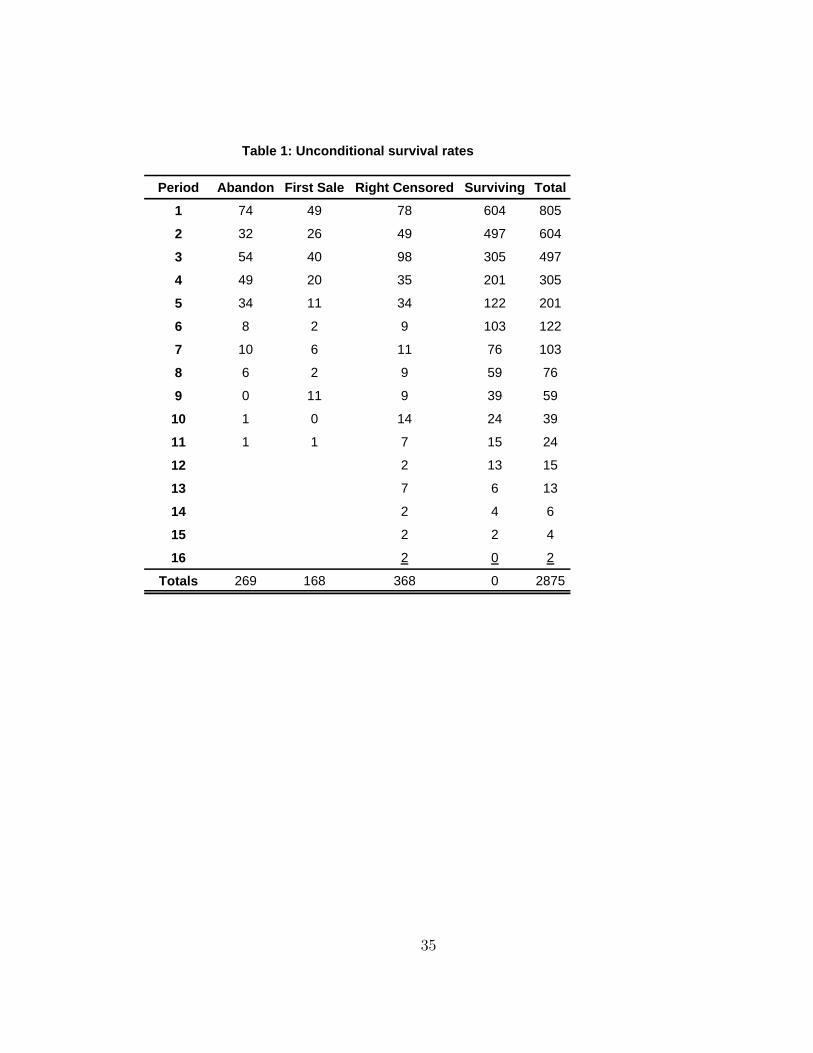
Period Abandon First Sale Right Censored Surviving Total

1 74 49 78 604 805

2 32 26 49 497 604

3 54 40 98 305 497

4 49 20 35 201 305

5 34 11 34 122 201

6 8 2 9 103 122

7 10 6 11 76 103

8 6 2 9 59 76

9 0 11 9 39 59

10 1 0 14 24 39

11 1 1 7 15 24

12 2 13 15

13 7 6 13

14 2 4 6

15 2 2 4

16 2 0 2

Totals 269 168 368 0 2875

Table 1: Unconditional survival rates

35

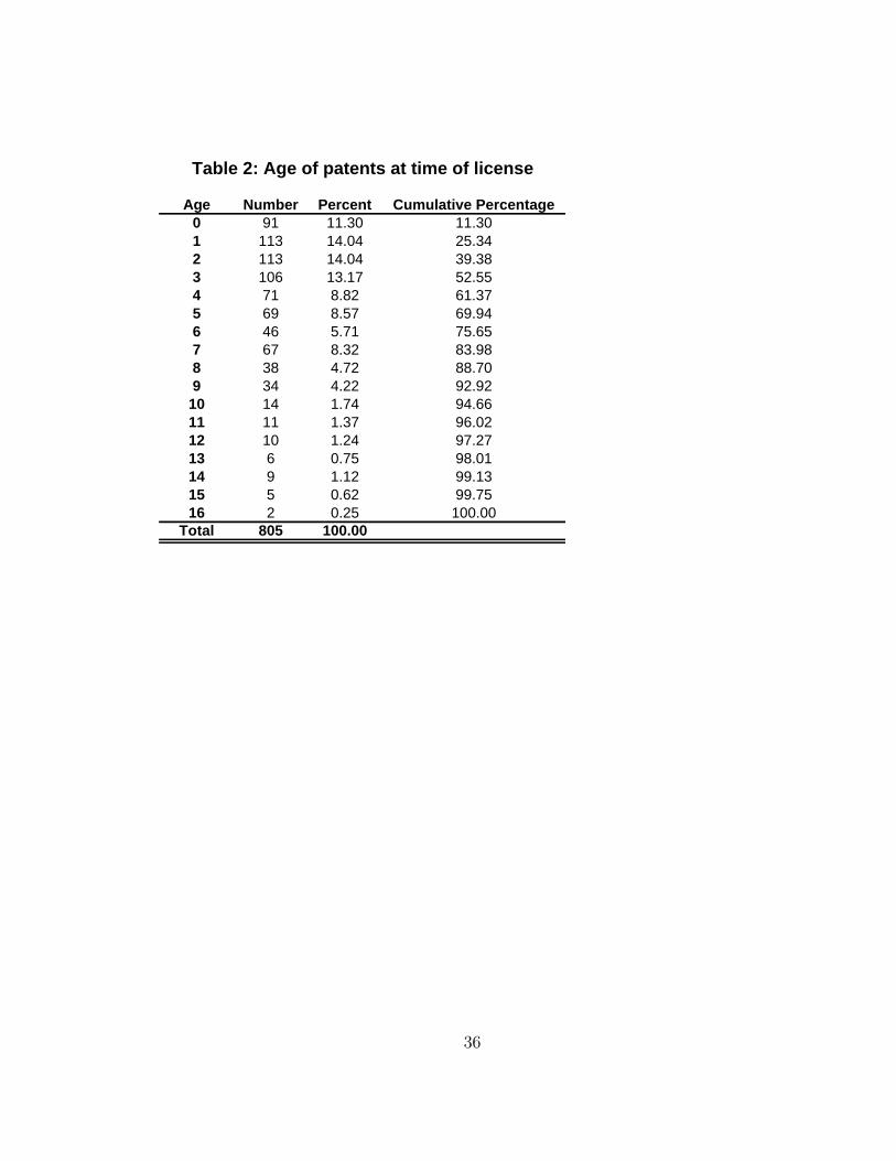
Age Number Percent Cumulative Percentage0 91 11.30 11.301 113 14.04 25.342 113 14.04 39.383 106 13.17 52.554 71 8.82 61.375 69 8.57 69.946 46 5.71 75.657 67 8.32 83.988 38 4.72 88.709 34 4.22 92.9210 14 1.74 94.6611 11 1.37 96.0212 10 1.24 97.2713 6 0.75 98.0114 9 1.12 99.1315 5 0.62 99.7516 2 0.25 100.00

Total 805 100.00

Table 2: Age of patents at time of license

36

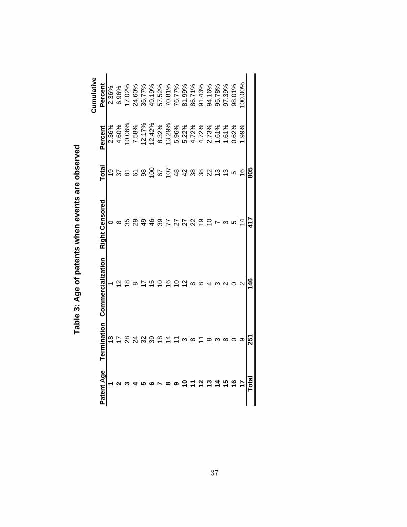
Pat

ent

Ag

eT

erm

inat

ion

Co

mm

erci

aliz

atio

nR

igh

t C

enso

red

To

tal

Per

cen

tC

um

ula

tive

P

erce

nt

118

10

192.

36%

2.36

%2

1712

837

4.60

%6.

96%

328

1835

8110

.06%

17.0

2%4

248

2961

7.58

%24

.60%

532

1749

9812

.17%

36.7

7%6

3915

4610

012

.42%

49.1

9%7

1810

3967

8.32

%57

.52%

814

1677

107

13.2

9%70

.81%

911

1027

485.

96%

76.7

7%10

312

2742

5.22

%81

.99%

118

822

384.

72%

86.7

1%12

118

1938

4.72

%91

.43%

138

410

222.

73%

94.1

6%14

33

713

1.61

%95

.78%

158

23

131.

61%

97.3

9%16

00

55

0.62

%98

.01%

179

214

161.

99%

100.

00%

To

tal

251

146

417

805

Tab

le 3

: A

ge

of

pat

ents

wh

en e

ven

ts a

re o

bse

rved

37

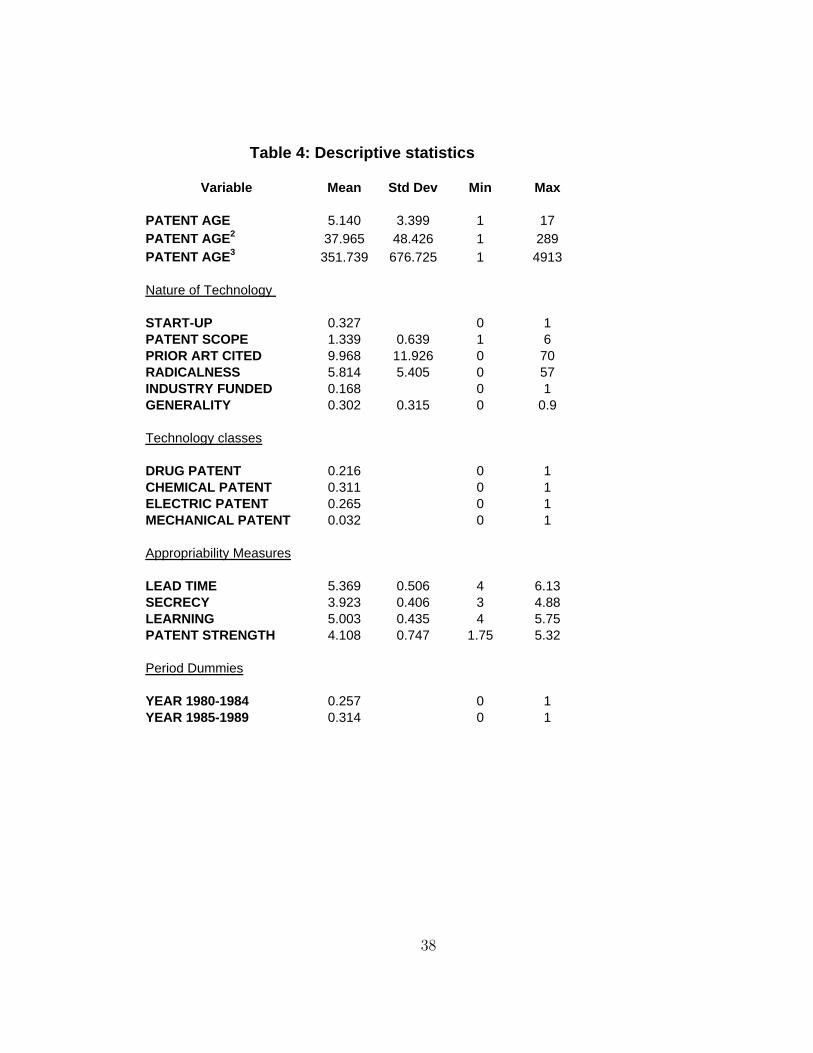
Variable Mean Std Dev Min Max

PATENT AGE 5.140 3.399 1 17PATENT AGE2 37.965 48.426 1 289PATENT AGE3 351.739 676.725 1 4913

Nature of Technology

START-UP 0.327 0 1PATENT SCOPE 1.339 0.639 1 6PRIOR ART CITED 9.968 11.926 0 70RADICALNESS 5.814 5.405 0 57INDUSTRY FUNDED 0.168 0 1GENERALITY 0.302 0.315 0 0.9

Technology classes

DRUG PATENT 0.216 0 1CHEMICAL PATENT 0.311 0 1ELECTRIC PATENT 0.265 0 1MECHANICAL PATENT 0.032 0 1

Appropriability Measures

LEAD TIME 5.369 0.506 4 6.13SECRECY 3.923 0.406 3 4.88LEARNING 5.003 0.435 4 5.75PATENT STRENGTH 4.108 0.747 1.75 5.32

Period Dummies

YEAR 1980-1984 0.257 0 1YEAR 1985-1989 0.314 0 1

Table 4: Descriptive statistics

38

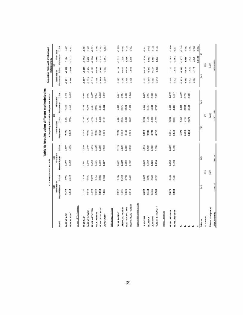
NA

ME

Haz

ard

Rat

ioZ

-Sta

tH

azar

d R

atio

Z-S

tat

Par

amet

erZ

-Sta

tP

aram

eter

Z-S

tat

Par

amet

erZ

-Sta

tP

aram

eter

Z-S

tat

PA

TE

NT

AG

E0.

769

-3.9

901.

208

2.18

0-0

.300

-3.6

610.

156

1.47

6-0

.271

-2.5

790.

194

1.46

0

PA

TE

NT

AG

E2

1.01

33.

110

0.99

2-1

.380

0.01

94.

030

-0.0

06-0

.983

0.01

52.

548

-0.0

11-1

.401

Nat

ure

of T

echn

olog

y

ST

AR

T-U

P1.

230

1.51

01.

101

0.53

00.

048

0.28

20.

193

0.95

7-1

.197

-5.3

23-0

.350

-1.3

11

PA

TE

NT

SC

OP

E0.

943

-0.5

401.

345

2.84

0-0

.092

-0.7

670.

277

2.04

0-0

.079

-0.4

340.

492

2.90

3

PR

IOR

AR

T C

ITE

D1.

002

0.18

00.

982

-1.2

600.

014

1.39

9-0

.017

-0.9

69-0

.015

-1.0

26-0

.050

-2.5

03

RA

DIC

AL

NE

SS

0.99

2-0

.450

1.02

10.

820

-0.0

08-0

.507

0.02

60.

959

0.02

80.

994

0.07

92.

342

IND

US

TR

Y F

UN

DE

D0.

658

-2.0

801.

069

0.29

0-0

.354

-1.5

78-0

.064

-0.2

32-0

.609

-1.9

80-0

.335

-0.9

52

GE

NE

RA

LIT

Y1.

881

2.63

00.

427

-2.9

000.

029

0.10

5-0

.642

-2.1

92-0

.199

-0.5

30-0

.661

-1.6

13

Tec

hnol

ogy

clas

ses

DR

UG

PA

TE

NT

0.86

7-0

.420

0.71

6-0

.740

-0.0

48-0

.117

-0.1

88-0

.337

0.09

70.

139

-0.5

22-0

.725

CH

EM

ICA

L P

AT

EN

T1.

091

0.36

02.

029

2.12

00.

158

0.60

20.

676

1.94

30.

149

0.40

70.

299

0.69

2

EL

EC

TR

IC P

AT

EN

T0.

826

-0.7

901.

959

1.88

0-0

.166

-0.6

260.

521

1.40

00.

326

0.88

41.

465

3.11

5

ME

CH

AN

ICA

L P

AT

EN

T0.

810

-0.4

800.

832

-0.2

300.

026

0.06

5-0

.112

-0.1

461.

028

1.80

21.

376

1.31

0

App

ropr

iabi

lity

Mea

sure

s

LE

AD

TIM

E2.

389

3.12

00.

528

-1.8

500.

883

3.33

1-0

.622

-1.6

060.

161

0.43

5-1

.136

-2.1

41

SE

CR

EC

Y0.

444

-3.2

401.

612

1.43

0-0

.930

-3.5

400.

495

1.22

3-0

.856

-2.2

721.

082

2.01

6

LE

AR

NIN

G0.

461

-2.5

603.

020

2.58

0-0

.723

-2.3

801.

043

2.09

90.

053

0.12

71.

353

2.11

3

PA

TE

NT

ST

RE

NG

TH

0.58

9-3

.250

2.21

63.

030

-0.7

10-3

.805

0.75

62.

388

-0.8

42-2

.961

1.22

33.

108

Per

iod

Dum

mie

s

YE

AR

198

0-19

840.

276

-2.1

601.

662

1.21

00.

061

0.23

1-0

.365

-1.6

400.

415

1.12

0-0

.093

-0.3

30

YE

AR

198

5-19

890.

630

-2.4

401.

393

1.59

00.

648

3.39

7-1

.147

-4.3

070.

503

1.85

0-1

.781

-5.5

77

� 1i

-1.3

78-4

.226

-0.8

08-2

.099

-2.9

23-3

.590

-1.7

77-3

.045

� 2i3.

704

5.71

22.

004

2.77

09.

441

4.53

75.

958

4.48

2

� 1i0.

234

2.87

10.

100

2.33

40.

002

1.52

10.

001

1.22

0

� 2i1.

087

1.47

40.

305

1.81

6

qi

0.54

302.

807

Fai

lure

s

# L

icen

ses

Tim

e at

ris

k (y

ears

)

Lo

g L

ikel

iho

od

Ter

min

atio

nF

irst

Sal

e

243

145

805

2403

-145

9.19

-881

.74

Ter

min

atio

nF

irst

Sal

e

-108

7.14

54

805

2403

243

145

Co

mp

etin

g R

isks

wit

h In

dep

end

ent

Ris

ksC

om

pet

ing

Ris

ks w

ith

Un

ob

serv

ed

Het

ero

gen

eity

(a1)

(a2)

(b)

Tab

le 5

: R

esu

lts

usi

ng

dif

fere

nt

met

ho

do

log

ies

-105

5.53

20

243

145

805

2403

(c)

Ter

min

atio

nF

irst

Sal

e

Co

x P

rop

ort

ion

al H

azar

ds

39

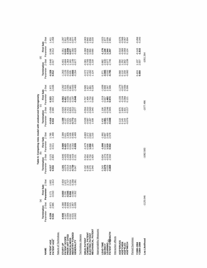
NA

ME

Par

amet

erZ

-Sta

tP

aram

eter

Z-S

tat

Par

amet

erZ

-Sta

tP

aram

eter

Z-S

tat

Par

amet

erZ

-Sta

tP

aram

eter

Z-S

tat

Par

amet

erZ

-Sta

tP

aram

eter

Z-S

tat

PA

TE

NT

AG

E-0

.339

-3.6

710.

171

1.60

2-0

.317

-3.1

210.

210

1.78

5-0

.416

-3.4

560.

323

1.97

2-0

.328

-2.6

400.

248

1.41

1P

AT

EN

T A

GE

20.

016

2.98

5-0

.010

-1.6

120.

016

2.80

4-0

.011

-1.4

900.

016

2.58

0-0

.012

-1.6

360.

012

2.01

7-0

.012

-1.4

58

Nat

ure

of T

echn

olog

y

ST

AR

T-U

P-0

.936

-4.3

80-0

.650

-2.9

34-1

.101

-4.8

46-0

.580

-2.3

89-1

.159

-4.9

26-0

.561

-2.2

62-1

.263

-5.4

01-0

.351

-1.2

87P

AT

EN

T S

CO

PE

-0.1

67-0

.998

0.29

51.

872

-0.0

79-0

.425

0.42

32.

611

-0.1

07-0

.561

0.42

12.

519

-0.1

26-0

.684

0.51

02.

912

PR

IOR

AR

T C

ITE

D-0

.009

-0.8

05-0

.045

-2.7

27-0

.014

-1.0

33-0

.034

-1.8

35-0

.021

-1.4

11-0

.030

-1.5

55-0

.020

-1.3

64-0

.048

-2.2

99R

AD

ICA

LN

ES

S0.

032

1.51

50.

058

2.01

40.

018

0.64

80.

034

1.10

90.

025

0.82

90.

031

0.98

10.

035

1.16

30.

077

2.18

4IN

DU

ST

RY

FU

ND

ED

-0.5

31-1

.957

-0.0

80-0

.268

-0.7

39-2

.419

-0.1

62-0

.485

-0.7

73-2

.512

-0.1

87-0

.543

-0.6

66-2

.149

-0.3

50-0

.977

GE

NE

RA

LIT

Y-0

.002

-0.0

05-0

.352

-1.0

610.

047

0.13

1-0

.935

-2.4

690.

028

0.07

7-0

.948

-2.4

69-0

.264

-0.6

77-0

.628

-1.4

94

Tec

hnol

ogy

clas

ses

DR

UG

PA

TE

NT

0.15

20.

214

-0.4

79-0

.683

-0.5

39-0

.554

0.70

70.

589

-0.3

72-0

.381

-0.3

69-0

.303

CH

EM

ICA

L P

AT

EN

T0.

185

0.49

30.

556

1.37

2-0

.587

-1.0

101.

409

1.62

7-0

.411

-0.7

050.

838

0.94

0E

LE

CT

RIC

PA

TE

NT

0.27

00.

734

1.05

82.

662

-0.4

97-0

.943

1.73

41.

861

-0.4

92-0

.938

1.95

01.

956

ME

CH

AN

ICA

L P

AT

EN

T1.

040

1.82

51.

189

1.21

51.

038

1.04

50.

665

0.22

81.

124

1.21

80.

690

0.23

3

App

ropr

iabi

lity

Mea

sure

s

LE

AD

TIM

E0.

243

0.63

4-1

.006

-1.9

910.

430

1.10

6-1

.019

-1.8

380.

371

0.98

2-1

.176

-2.0

23S

EC

RE

CY

-0.8

79-2

.273

0.52

20.

997

-0.9

81-2

.554

0.55

70.

999

-0.9

95-2

.630

1.10

91.

977

LE

AR

NIN

G-0

.033

-0.0

781.

519

2.40

0-0

.105

-0.2

481.

483

2.26

7-0

.032

-0.0

771.

344

2.03

9P

AT

EN

T S

TR

EN

GT

H-0

.869

-2.9

320.

932

2.57

8-0

.848

-2.8

050.

974

2.58

6-0

.795

-2.7

461.

207

2.98

1

Inte

ract

ion

effe

cts

AG

E*D

RU

GS

0.11

00.

975

-0.1

55-1

.279

0.06

80.

594

-0.0

10-0

.076

AG

E*C

HE

M0.

145

1.60

0-0

.104

-0.9

370.

110

1.25

2-0

.069

-0.5

68A

GE

*EL

EC

0.14

41.

631

-0.0

66-0

.556

0.15

91.

842

-0.0

59-0

.457

AG

E*M

EC

H-0

.076

-0.2

170.

121

0.30

6-0

.082

-0.2

390.

124

0.30

4

Per

iod

Dum

mie

s

Y19

80-1

984

0.42

41.

137

-0.1

43-0

.494

Y19

84-1

989

0.56

02.

007

-1.8

15-5

.343

Lo

g L

ikel

iho

od

Ter

min

atio

nT

erm

inat

ion

Fir

st S

ale

-108

2.58

3-1

125.

046

Ter

min

atio

nF

irst

Sal

eF

irst

Sal

e

-107

7.48

6-1

051.

264

Ter

min

atio

nF

irst

Sal

e

Tab

le 6

: C

om

pet

ing

ris

ks m

od

el w

ith

un

ob

serv

ed h

eter

og

enei

ty(a

)(b

)(c

)(d

)

40

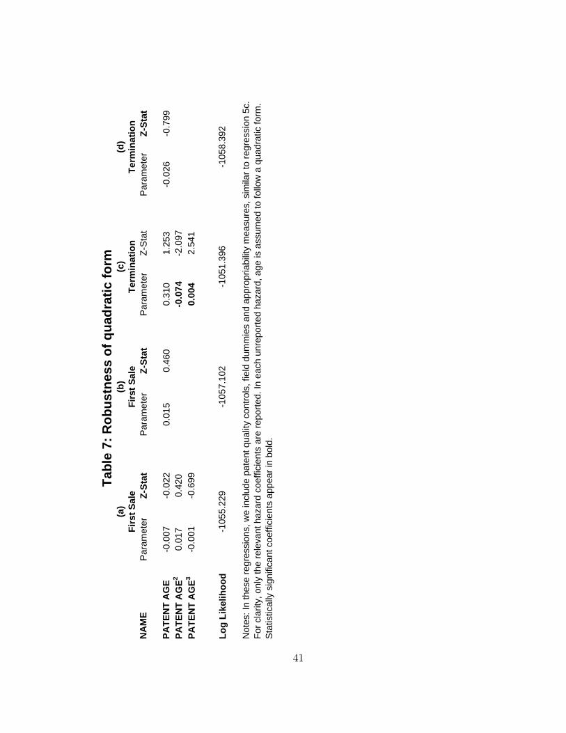
NA

ME

Par

amet

erZ

-Sta

tP

aram

eter

Z-S

tat

Par

amet

erZ

-Sta

tP

aram

eter

Z-S

tat

PA

TE

NT

AG

E-0

.007

-0.0

220.

015

0.46

00.

310

1.25

3-0

.026

-0.7

99P

AT

EN

T A

GE

20.

017

0.42

0-0

.074

-2.0

97P

AT

EN

T A

GE

3-0

.001

-0.6

990.

004

2.54

1

Lo

g L

ikel

iho

od

Fir

st S

ale

Fir

st S

ale

Ter

min

atio

n

-105

1.39

6

Ter

min

atio

n

Not

es: I

n th

ese

regr

essi

ons,

we

incl

ude

pate

nt q

ualit

y co

ntro

ls, f

ield

dum

mie

s an

d ap

prop

riabi

lity

mea

sure

s, s

imila

r to

reg

ress

ion

5c.

For

cla

rity,

onl

y th

e re

leva

nt h

azar

d co

effic

ient

s ar

e re

port

ed. I

n ea

ch u

nrep

orte

d ha

zard

, age

is a

ssum

ed to

follo

w a

qua

drat

ic fo

rm.

Sta

tistic

ally

sig

nific

ant c

oeffi

cien

ts a

ppea

r in

bol

d.

Tab

le 7

: R

ob

ust

nes

s o

f q

uad

rati

c fo

rm

-105

8.39

2

(a)

(b)

(c)

(d)

-105

5.22

9-1

057.

102

41

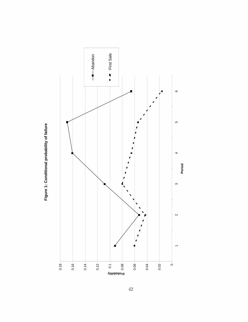
Fig

ure

1:

Co

nd

itio

nal

pro

bab

ility

of

failu

re

0

0.02

0.04

0.06

0.080.1

0.12

0.14

0.16

0.18

12

34

56

Per

iod

Probability

Aba

ndon

Firs

t Sal

e

42

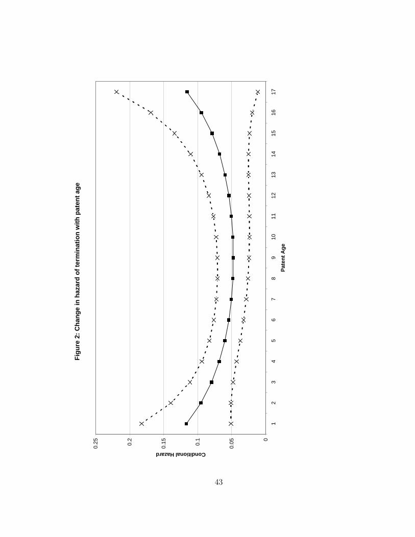
Fig

ure

2:

Ch

ang

e in

haz

ard

of

term

inat

ion

wit

h p

aten

t ag

e

0

0.050.1

0.150.2

0.25

12

34

56

78

910

1112

1314

1516

17

Pat

ent

Ag

e

Conditional Hazard

43

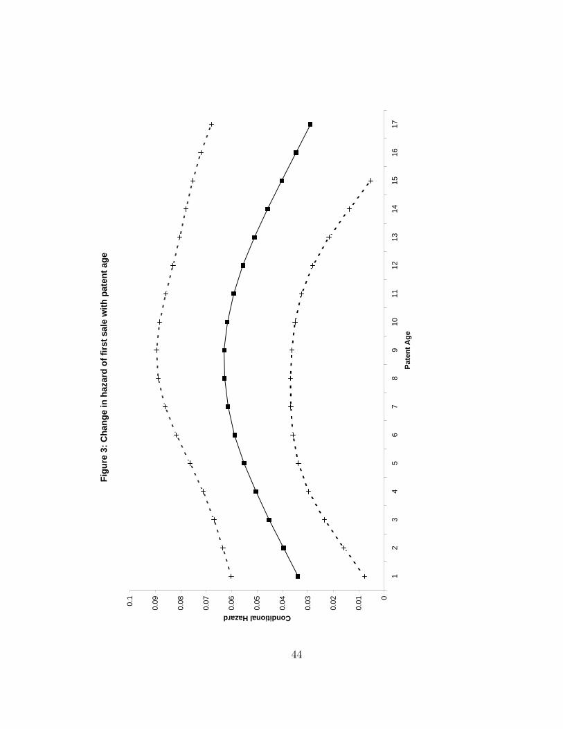
Fig

ure

3:

Ch

ang

e in

haz

ard

of

firs

t sa

le w

ith

pat

ent

age

0

0.01

0.02

0.03

0.04

0.05

0.06

0.07

0.08

0.090.1

12

34

56

78

910

1112

1314

1516

17

Pat

ent

Ag

e

Conditional Hazard

44