Embed Size (px)
Citation preview
Lukáš Sekanina Faculty of Information Technology
Brno University of Technology Brno, Czech Republic [email protected]
Approximate Computing with
Approximate Circuits: Methodologies and Applications
ESWEEK 2017 Tutorial
Jie Han Department of Electrical and Computer
Engineering, University of Alberta Edmonton, AB, Canada
Lukáš Sekanina Faculty of Information Technology
Brno University of Technology Brno, Czech Republic [email protected]
Approximate Computing with
Approximate Circuits: Methodologies and Applications
Part II: Design automation methods
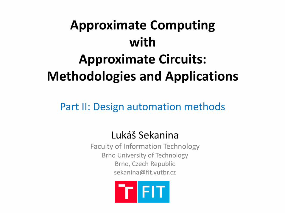
• Introduction • Design automation methods for approximate circuits
– Classification and overview – Circuit parameter estimation – Error computation – Relaxed equivalence checking – Evaluation methodology
• Examples of design automation methods for approximate circuits – Minterm complements, SASIMI, AIG rewriting, ABACUS, GRATER
• Evolutionary algorithms, CGP and circuit optimization • Applications of CGP-based approximation methods
– Open-source library of approximate adders and multipliers – Approximate TMR – Approximate multipliers in neural networks – Symbolic error analysis using BDDs/SAT solving in CGP-based tools – Approximate image filters
• Conclusions
Tutorial Outline – Part II.
3
Sensitivity analysis
4
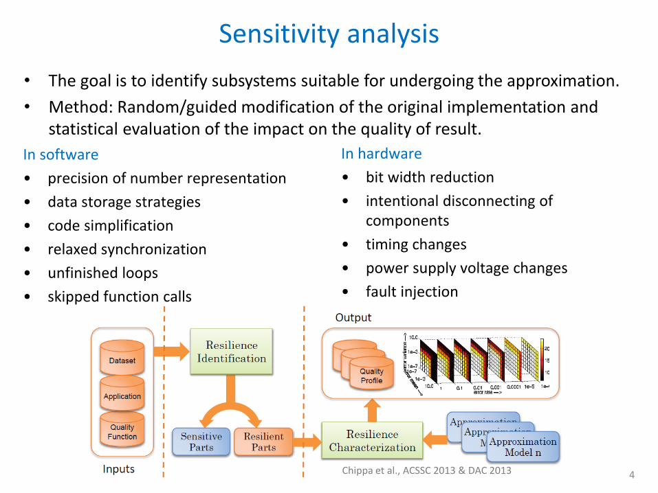
• The goal is to identify subsystems suitable for undergoing the approximation.
• Method: Random/guided modification of the original implementation and statistical evaluation of the impact on the quality of result.
In software
• precision of number representation
• data storage strategies
• code simplification
• relaxed synchronization
• unfinished loops
• skipped function calls
In hardware
• bit width reduction
• intentional disconnecting of components
• timing changes
• power supply voltage changes
• fault injection
Chippa et al., ACSSC 2013 & DAC 2013
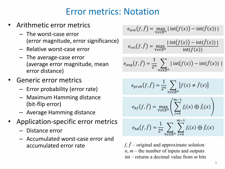
• Arithmetic error metrics – The worst-case error
(error magnitude, error significance)
– Relative worst-case error
– The average-case error (average error magnitude, mean error distance)
• Generic error metrics – Error probability (error rate)
– Maximum Hamming distance (bit-flip error)
– Average Hamming distance
• Application-specific error metrics – Distance error
– Accumulated worst-case error and accumulated error rate
Error metrics: Notation
5
𝑒𝑤𝑠𝑡 𝑓, 𝑓 = max∀𝑥∈ℬ𝑛
| int 𝑓 𝑥 − int(𝑓 𝑥 ) |
𝑒𝑟𝑒𝑙 𝑓, 𝑓 = max∀𝑥∈ℬ𝑛
| int 𝑓 𝑥 − int(𝑓 𝑥 ) |
int(𝑓 𝑥 )
𝑒𝑎𝑣𝑔 𝑓, 𝑓 =1
2𝑛 | int 𝑓 𝑥 − int(𝑓 𝑥 )
∀𝑥∈ℬ𝑛
|
𝑒𝑝𝑟𝑜𝑏 𝑓, 𝑓 =1
2𝑛 𝑓 𝑥 ≠ 𝑓 (𝑥)
∀𝑥∈ℬ𝑛
𝑒𝑏𝑓 𝑓, 𝑓 = max∀𝑥∈ℬ𝑛
𝑓𝑖 𝑥 ⊕ 𝑓 𝑖(𝑥)
𝑚−1
𝑖=0
𝑒ℎ𝑑 𝑓, 𝑓 =1
2𝑛 𝑓𝑖 𝑥 ⊕ 𝑓 𝑖(𝑥)
𝑚−1
𝑖=0∀𝑥∈ℬ𝑛
f, 𝑓 – original and approximate solution
n, m – the number of inputs and outputs
int – returns a decimal value from m bits
Approximation techniques - examples
6
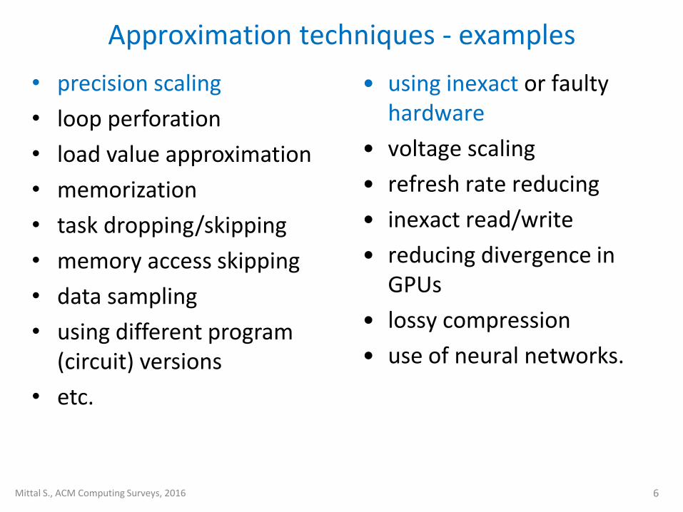
• precision scaling
• loop perforation
• load value approximation
• memorization
• task dropping/skipping
• memory access skipping
• data sampling
• using different program (circuit) versions
• etc.
• using inexact or faulty hardware
• voltage scaling
• refresh rate reducing
• inexact read/write
• reducing divergence in GPUs
• lossy compression
• use of neural networks.
Mittal S., ACM Computing Surveys, 2016
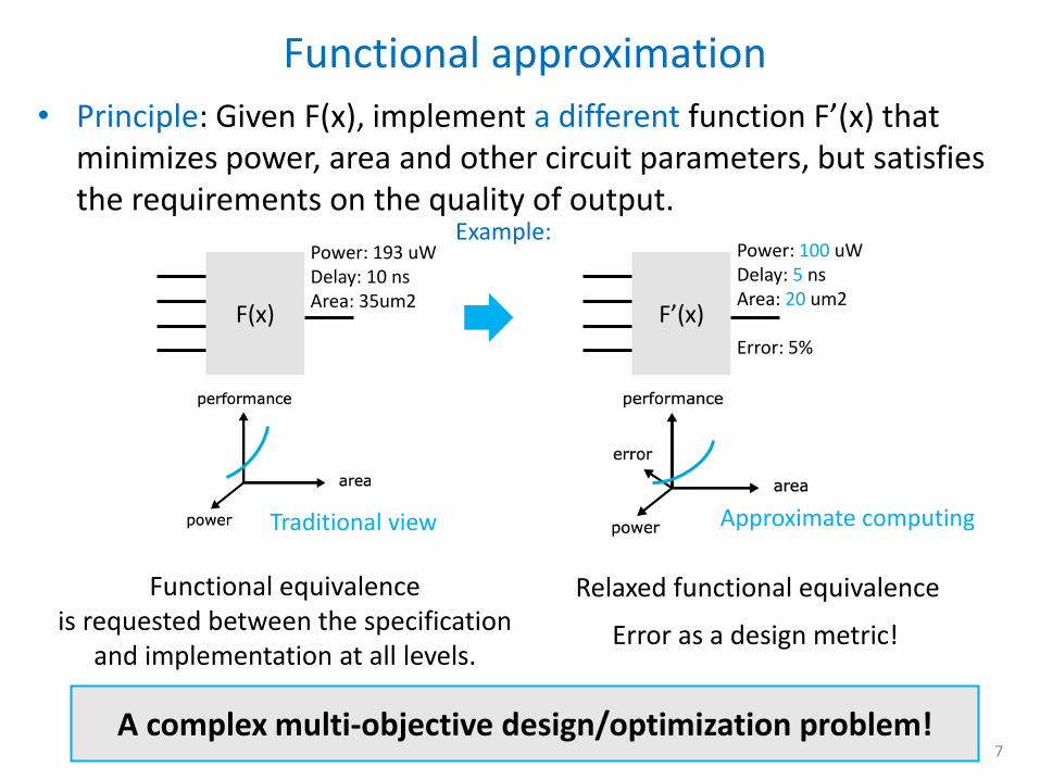
• Principle: Given F(x), implement a different function F’(x) that minimizes power, area and other circuit parameters, but satisfies the requirements on the quality of output.
Functional approximation
7
F(x) F’(x)
Power: 193 uW Delay: 10 ns Area: 35um2
Power: 100 uW Delay: 5 ns Area: 20 um2 Error: 5%
Traditional view Approximate computing
Functional equivalence is requested between the specification
and implementation at all levels. Error as a design metric!
Relaxed functional equivalence
A complex multi-objective design/optimization problem!
Example:
• Introduction • Design automation methods for approximate circuits
– Classification and overview – Circuit parameter estimation – Error computation – Relaxed equivalence checking – Evaluation methodology
• Examples of design automation methods for approximate circuits – Minterm complements, SASIMI, AIG rewriting, ABACUS, GRATER
• Evolutionary algorithms, CGP and circuit optimization • Applications of CGP-based approximation methods
– Open-source library of approximate adders and multipliers – Approximate TMR – Approximate multipliers in neural networks – Symbolic error analysis using BDDs/SAT solving in CGP-based tools – Approximate image filters
• Conclusions
Tutorial Outline – Part II.
8
Languages supporting approximate computing
9
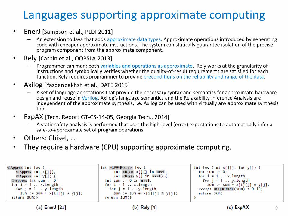
• EnerJ [Sampson et al., PLDI 2011] – An extension to Java that adds approximate data types. Approximate operations introduced by generating
code with cheaper approximate instructions. The system can statically guarantee isolation of the precise program component from the approximate component.
• Rely [Carbin et al., OOPSLA 2013] – Programmer can mark both variables and operations as approximate. Rely works at the granularity of
instructions and symbolically verifies whether the quality-of-result requirements are satisfied for each function. Rely requires programmer to provide preconditions on the reliability and range of the data.
• Axilog [Yazdanbakhsh et al., DATE 2015] – A set of language annotations that provide the necessary syntax and semantics for approximate hardware
design and reuse in Verilog. Axilog’s language semantics and the Relaxability Inference Analysis are independent of the approximate synthesis, i.e. Axilog can be used with virtually any approximate synthesis tool.
• ExpAX [Tech. Report GT-CS-14-05, Georgia Tech., 2014] – A static safety analysis is performed that uses the high-level (error) expectations to automatically infer a
safe-to-approximate set of program operations
• Others: Chisel, … • They require a hardware (CPU) supporting approximate computing.
Functional approximation of digital circuits
10
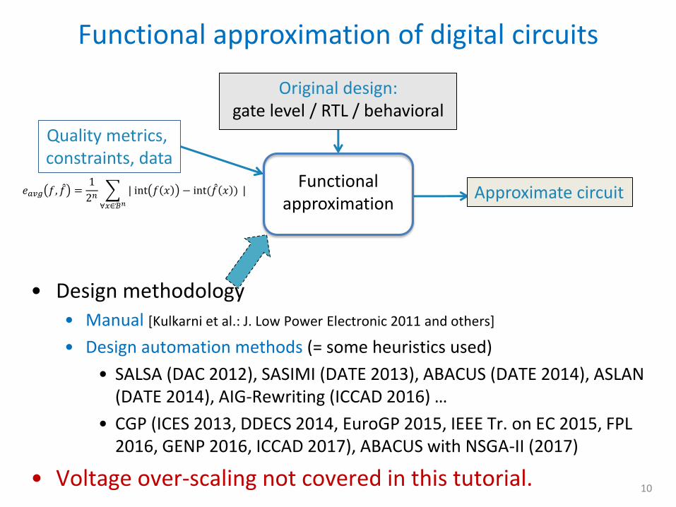
Functional approximation
Original design: gate level / RTL / behavioral
Approximate circuit 𝑒𝑎𝑣𝑔 𝑓, 𝑓 =1
2𝑛 | int 𝑓 𝑥 − int(𝑓 𝑥 )
∀𝑥∈ℬ𝑛
|
Quality metrics, constraints, data
• Design methodology • Manual [Kulkarni et al.: J. Low Power Electronic 2011 and others]
• Design automation methods (= some heuristics used)
• SALSA (DAC 2012), SASIMI (DATE 2013), ABACUS (DATE 2014), ASLAN (DATE 2014), AIG-Rewriting (ICCAD 2016) …
• CGP (ICES 2013, DDECS 2014, EuroGP 2015, IEEE Tr. on EC 2015, FPL 2016, GENP 2016, ICCAD 2017), ABACUS with NSGA-II (2017)
• Voltage over-scaling not covered in this tutorial.
Functional circuit approximation: Classification
11
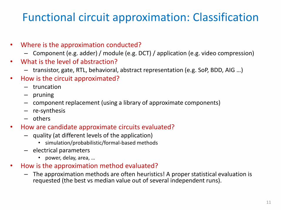
• Where is the approximation conducted? – Component (e.g. adder) / module (e.g. DCT) / application (e.g. video compression)
• What is the level of abstraction? – transistor, gate, RTL, behavioral, abstract representation (e.g. SoP, BDD, AIG …)
• How is the circuit approximated? – truncation – pruning – component replacement (using a library of approximate components) – re-synthesis – others
• How are candidate approximate circuits evaluated? – quality (at different levels of the application)
• simulation/probabilistic/formal-based methods
– electrical parameters • power, delay, area, …
• How is the approximation method evaluated? – The approximation methods are often heuristics! A proper statistical evaluation is
requested (the best vs median value out of several independent runs).
12
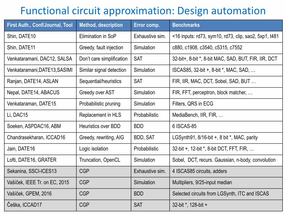
Functional circuit approximation: Design automation First Auth., Conf/Journal, Tool Method, description Error comp. Benchmarks
Shin, DATE10 Elimination in SoP Exhaustive sim. <16 inputs: rd73, sym10, rd73, clip, sao2, 5xp1, t481
Shin, DATE11 Greedy, fault injection Simulation c880, c1908, c3540, c5315, c7552
Venkataramani, DAC12, SALSA Don’t care simplification SAT 32-bit+, 8-bit *, 8-bit MAC, SAD, BUT, FIR, IIR, DCT
Venkataramani,DATE13,SASIMI Similar signal detection Simulation ISCAS85, 32-bit +, 8-bit *, MAC, SAD, …
Ranjan, DATE14, ASLAN Sequential/heuristics SAT FIR, IIR, MAC, DCT, Sobel, SAD, BUT …
Nepal, DATE14, ABACUS Greedy over AST Simulation FIR, FFT, perceptron, block matcher, …
Venkataraman, DATE15 Probabilistic pruning Simulation Filters, QRS in ECG
Li, DAC15 Replacement in HLS Probabilistic MediaBench, IIR, FIR, …
Soeken, ASPDAC16, ABM Heuristics over BDD BDD 6 ISCAS-85
Chandrasekharan, ICCAD16 Greedy, rewriting, AIG BDD, SAT LGSynth91, 8/16-bit +, 8 bit *, MAC, parity
Jain, DATE16 Logic isolation Probabilistic 32-bit +, 12-bit *, 8-bit DCT, FFT, FIR, …
Lofti, DATE16, GRATER Truncation, OpenCL Simulation Sobel, DCT, recurs. Gaussian, n-body, convolution
Sekanina, SSCI-ICES13 CGP Exhaustive sim. 4 ISCAS85 circuits, adders
Vašíček, IEEE Tr. on EC, 2015 CGP Simulation Multipliers, 9/25-input median
Vašíček, GPEM, 2016 CGP BDD Selected circuits from LGSynth, ITC and ISCAS
Češka, ICCAD17 CGP SAT 32-bit *, 128-bit +
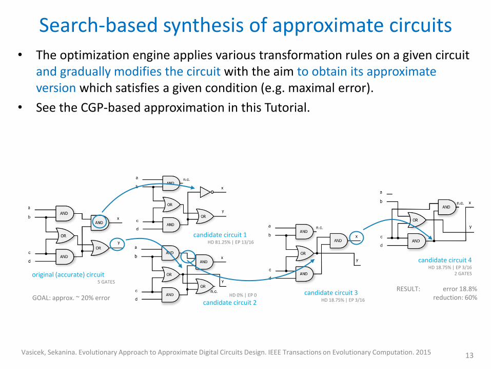
Search-based synthesis of approximate circuits
13
candidate circuit 3 HD 18.75% | EP 3/16
candidate circuit 1 HD 81.25% | EP 13/16
• The optimization engine applies various transformation rules on a given circuit and gradually modifies the circuit with the aim to obtain its approximate version which satisfies a given condition (e.g. maximal error).
• See the CGP-based approximation in this Tutorial.
Vasicek, Sekanina. Evolutionary Approach to Approximate Digital Circuits Design. IEEE Transactions on Evolutionary Computation. 2015
original (accurate) circuit 5 GATES
HD 0% | EP 0
candidate circuit 2
candidate circuit 4 HD 18.75% | EP 3/16
2 GATES
GOAL: approx. ~ 20% error RESULT: error 18.8%
reduction: 60%
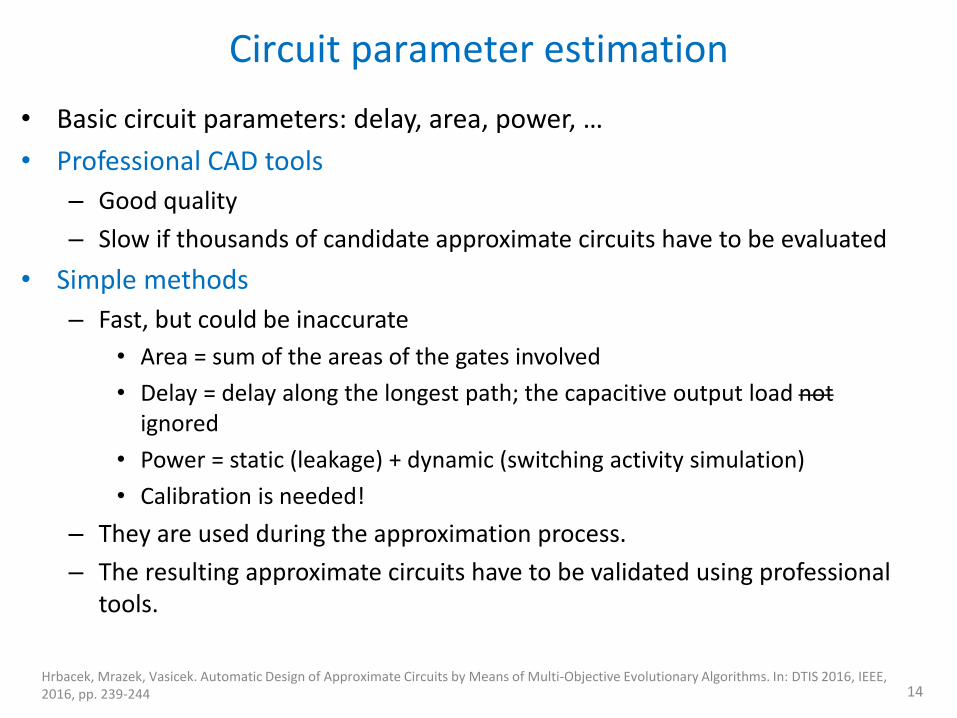
Circuit parameter estimation
14
• Basic circuit parameters: delay, area, power, …
• Professional CAD tools
– Good quality
– Slow if thousands of candidate approximate circuits have to be evaluated
• Simple methods
– Fast, but could be inaccurate
• Area = sum of the areas of the gates involved
• Delay = delay along the longest path; the capacitive output load not ignored
• Power = static (leakage) + dynamic (switching activity simulation)
• Calibration is needed!
– They are used during the approximation process.
– The resulting approximate circuits have to be validated using professional tools.
Hrbacek, Mrazek, Vasicek. Automatic Design of Approximate Circuits by Means of Multi-Objective Evolutionary Algorithms. In: DTIS 2016, IEEE, 2016, pp. 239-244
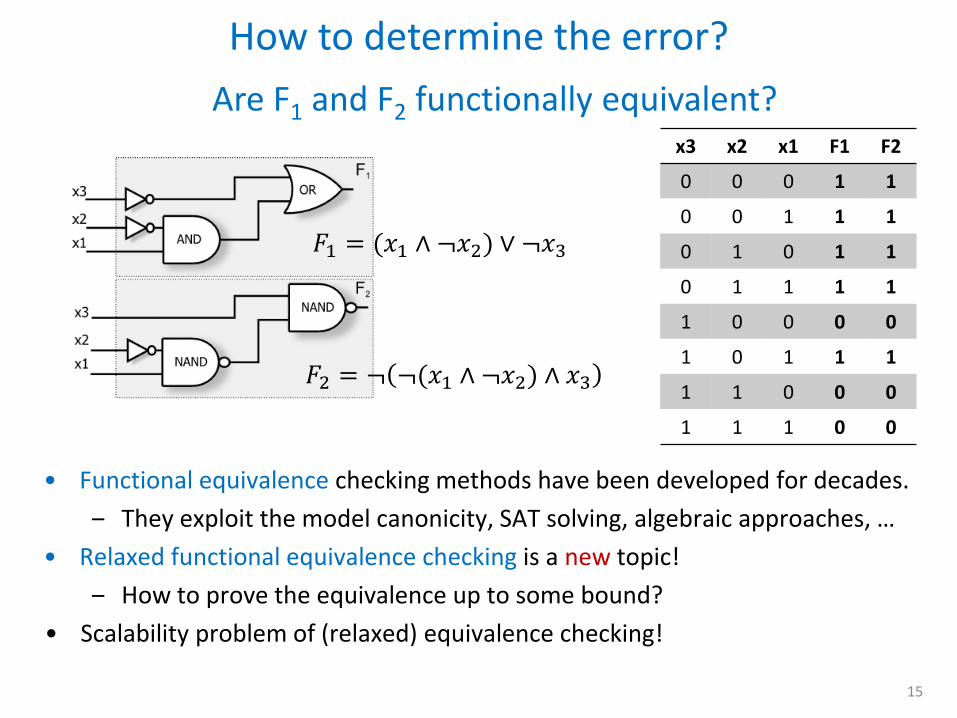
How to determine the error?
15
x3 x2 x1 F1 F2
0 0 0 1 1
0 0 1 1 1
0 1 0 1 1
0 1 1 1 1
1 0 0 0 0
1 0 1 1 1
1 1 0 0 0
1 1 1 0 0
• Functional equivalence checking methods have been developed for decades.
‒ They exploit the model canonicity, SAT solving, algebraic approaches, …
• Relaxed functional equivalence checking is a new topic!
‒ How to prove the equivalence up to some bound?
• Scalability problem of (relaxed) equivalence checking!
𝐹2 = ¬ ¬(𝑥1 ∧ ¬𝑥2) ∧ 𝑥3
𝐹1 = (𝑥1 ∧ ¬𝑥2) ∨ ¬𝑥3
Are F1 and F2 functionally equivalent?
How to determine the error?
16
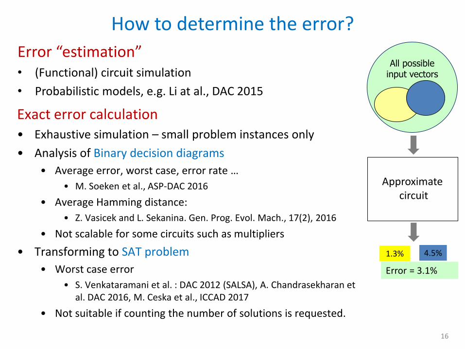
Error “estimation” • (Functional) circuit simulation
• Probabilistic models, e.g. Li at al., DAC 2015
All possible input vectors
Approximate circuit
1.3% 4.5%
Error = 3.1%
Exact error calculation • Exhaustive simulation – small problem instances only
• Analysis of Binary decision diagrams
• Average error, worst case, error rate …
• M. Soeken et al., ASP-DAC 2016
• Average Hamming distance:
• Z. Vasicek and L. Sekanina. Gen. Prog. Evol. Mach., 17(2), 2016
• Not scalable for some circuits such as multipliers
• Transforming to SAT problem
• Worst case error
• S. Venkataramani et al. : DAC 2012 (SALSA), A. Chandrasekharan et al. DAC 2016, M. Ceska et al., ICCAD 2017
• Not suitable if counting the number of solutions is requested.
Error computation: Probabilistic methods
17
• For a given approximate circuit and the input data distribution, a probabilistic model is constructed and the error statistics are derived.
• Examples – The error statistics can be expressed as functions of the number of input
bits, carry-chain length, number of overlapping prediction bits and number of sub-adders in the case of approximate adders [Mazahir et al. IEEE TC 66(3), 2017]
– In the context of approximate HLS, an error of approximate adders and multipliers was characterized by its mean and variance. The mean is systematic and can be compensated. The overall computation precision is then determined by the variance which, after the constant compensation corresponds, to the Mean Squared Error [Li et al. DAC 2015].
• Advantages – Fast error computation
• Disadvantages – An error model has to be derived for all components which is time
consuming and impractical for circuits different to adders and multipliers. – It is hard to provide formal guarantees in terms of the error bound.
Example [Li et al. DAC 2015]
18
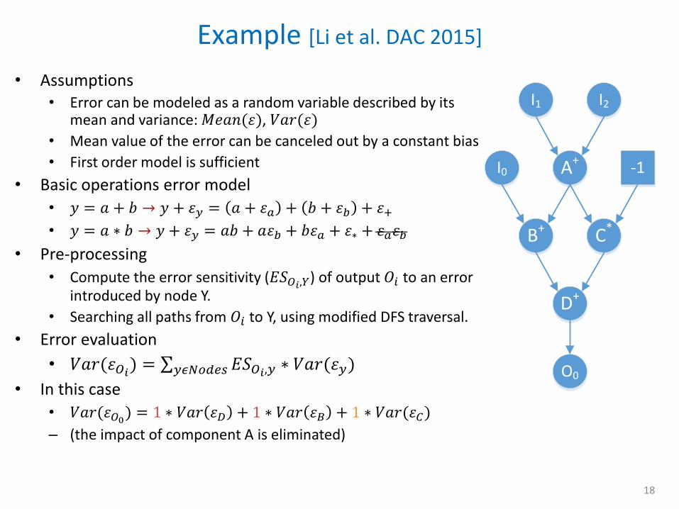
• Assumptions • Error can be modeled as a random variable described by its
mean and variance: 𝑀𝑒𝑎𝑛(𝜀), 𝑉𝑎𝑟(𝜀)
• Mean value of the error can be canceled out by a constant bias
• First order model is sufficient
• Basic operations error model
• 𝑦 = 𝑎 + 𝑏 → 𝑦 + 𝜀𝑦 = 𝑎 + 𝜀𝑎 + 𝑏 + 𝜀𝑏 + 𝜀+
• 𝑦 = 𝑎 ∗ 𝑏 → 𝑦 + 𝜀𝑦 = 𝑎𝑏 + 𝑎𝜀𝑏 + 𝑏𝜀𝑎 + 𝜀∗ + 𝜀𝑎𝜀𝑏
• Pre-processing
• Compute the error sensitivity (𝐸𝑆𝑂𝑖,𝑌) of output 𝑂𝑖 to an error
introduced by node Y.
• Searching all paths from 𝑂𝑖 to Y, using modified DFS traversal.
• Error evaluation
• 𝑉𝑎𝑟(𝜀𝑂𝑖) = 𝐸𝑆𝑂𝑖,𝑦 ∗ 𝑉𝑎𝑟(𝜀𝑦)𝑦𝜖𝑁𝑜𝑑𝑒𝑠
• In this case
• 𝑉𝑎𝑟(𝜀𝑂0) = 1 ∗ 𝑉𝑎𝑟 𝜀𝐷 + 1 ∗ 𝑉𝑎𝑟 𝜀𝐵 + 1 ∗ 𝑉𝑎𝑟(𝜀𝐶)
– (the impact of component A is eliminated)
I1 I2
A+
B+
I0
D+
C*
O0
-1
Binary Decision Diagrams
19
1 edge
0 edge
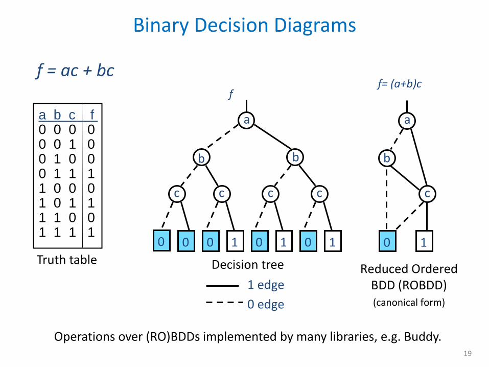
a b c f 0 0 0 0 0 0 1 0 0 1 0 0 0 1 1 1 1 0 0 0 1 0 1 1 1 1 0 0 1 1 1 1
Truth table
f = ac + bc
Decision tree
1 0 0 0 1 0 1 0
a
b
c
b
c c c
f
1 0
a
b
c
f= (a+b)c
Reduced Ordered BDD (ROBDD) (canonical form)
Operations over (RO)BDDs implemented by many libraries, e.g. Buddy.
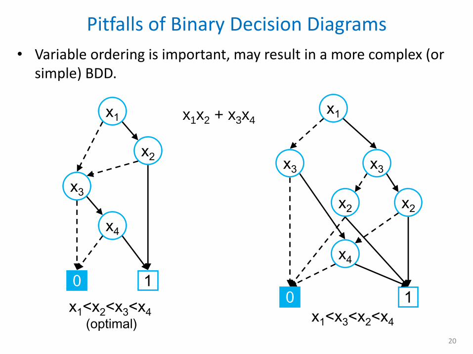
• Variable ordering is important, may result in a more complex (or simple) BDD.
Pitfalls of Binary Decision Diagrams
20
x1
x3
x4
0 1
x2
x1x2 + x3x4
x1<x2<x3<x4 (optimal)
x1<x3<x2<x4
x1
x3
x4
0 1
x2
x3
x2
The decision procedure is trivial and reduces to pointer comparison.
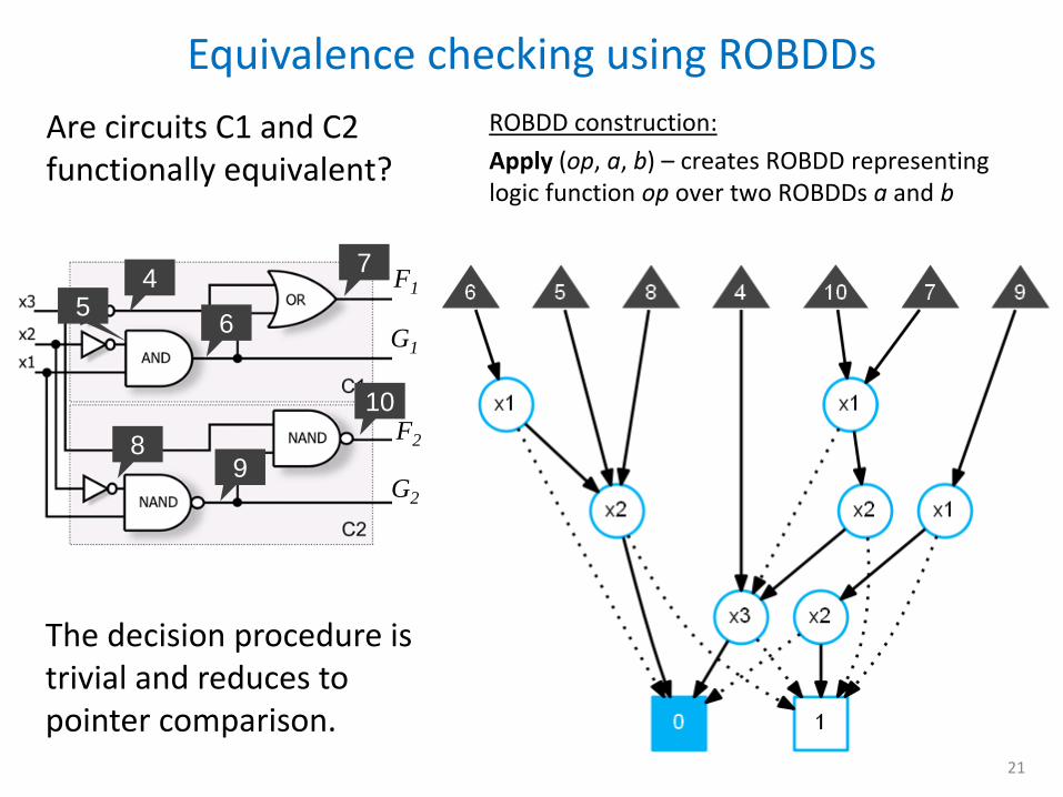
Equivalence checking using ROBDDs
21
F1
F2
G1
G2
4
6
7
8 9
10
5
ROBDD construction:
Apply (op, a, b) – creates ROBDD representing logic function op over two ROBDDs a and b
Are circuits C1 and C2 functionally equivalent?
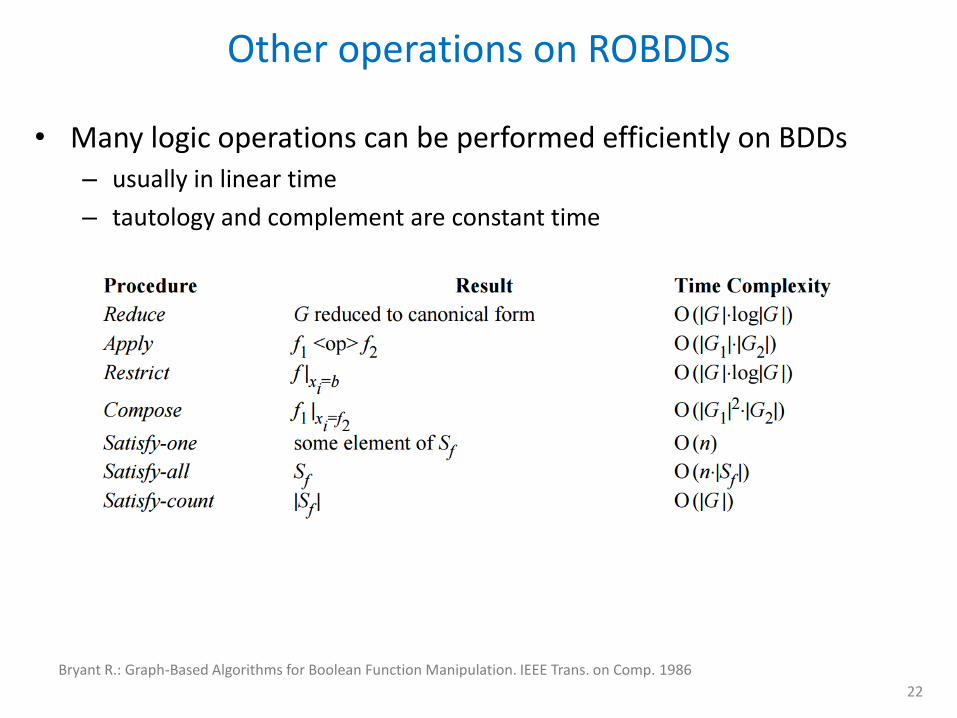
• Many logic operations can be performed efficiently on BDDs – usually in linear time
– tautology and complement are constant time
Other operations on ROBDDs
22
Bryant R.: Graph-Based Algorithms for Boolean Function Manipulation. IEEE Trans. on Comp. 1986
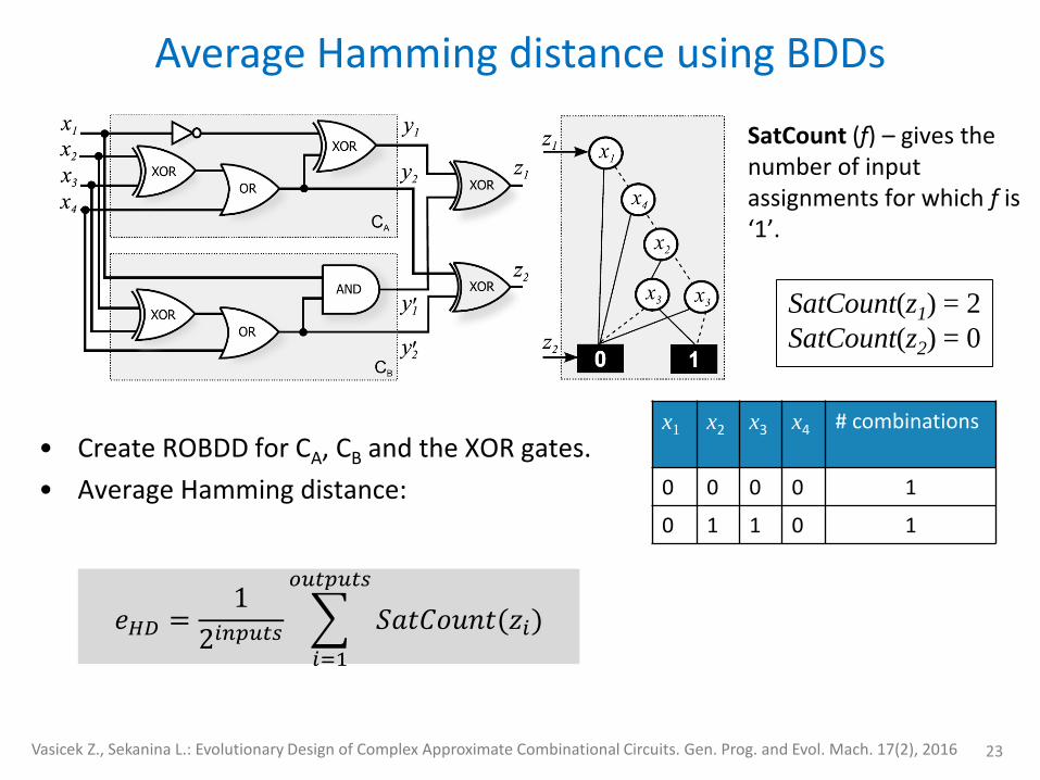
Average Hamming distance using BDDs
23
• Create ROBDD for CA, CB and the XOR gates.
• Average Hamming distance:
SatCount(z1) = 2
SatCount(z2) = 0
SatCount (f) – gives the number of input assignments for which f is ‘1’.
x1 x2 x3 x4 # combinations
0 0 0 0 1
0 1 1 0 1
𝑒𝐻𝐷 =1
2𝑖𝑛𝑝𝑢𝑡𝑠 𝑆𝑎𝑡𝐶𝑜𝑢𝑛𝑡(𝑧𝑖)
𝑜𝑢𝑡𝑝𝑢𝑡𝑠
𝑖=1
Vasicek Z., Sekanina L.: Evolutionary Design of Complex Approximate Combinational Circuits. Gen. Prog. and Evol. Mach. 17(2), 2016
Average-case and worst-case error analysis
24
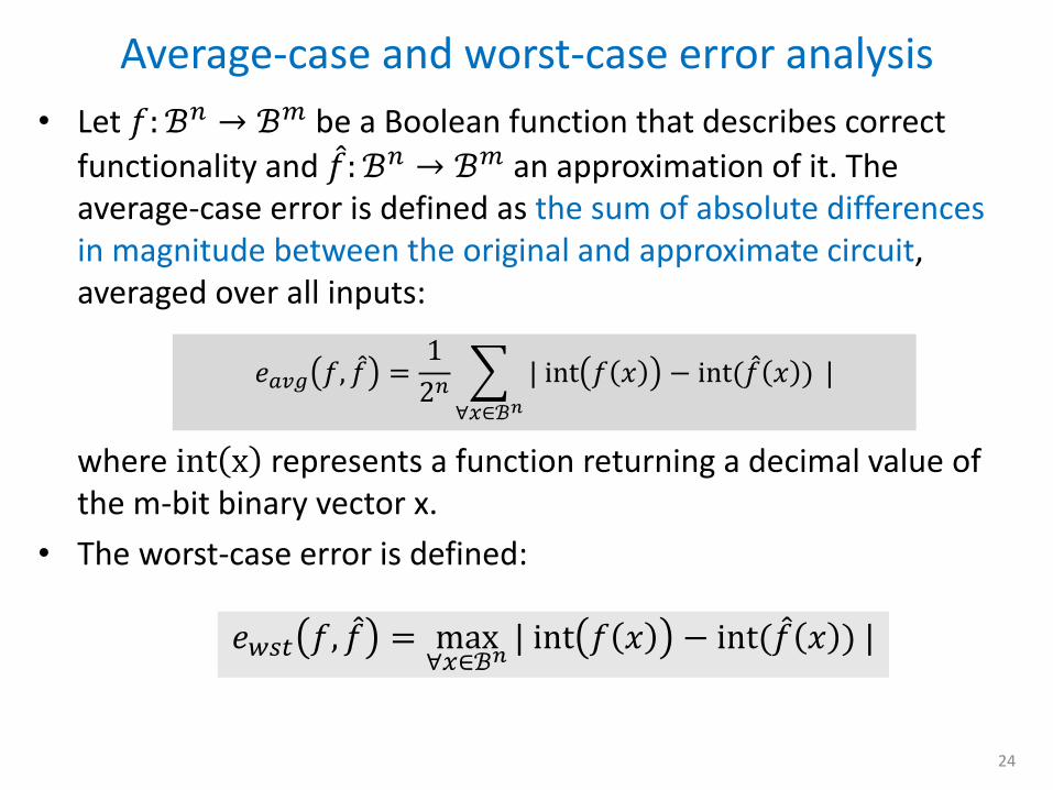
• Let 𝑓: ℬ𝑛 → ℬ𝑚 be a Boolean function that describes correct
functionality and 𝑓 : ℬ𝑛 → ℬ𝑚 an approximation of it. The average-case error is defined as the sum of absolute differences in magnitude between the original and approximate circuit, averaged over all inputs: where int x represents a function returning a decimal value of the m-bit binary vector x.
• The worst-case error is defined:
𝑒𝑎𝑣𝑔 𝑓, 𝑓 =1
2𝑛 | int 𝑓 𝑥 − int(𝑓 𝑥 )
∀𝑥∈ℬ𝑛
|
𝑒𝑤𝑠𝑡 𝑓, 𝑓 = max∀𝑥∈ℬ𝑛
| int 𝑓 𝑥 − int(𝑓 𝑥 ) |
Error analysis using BDD (adders)
25
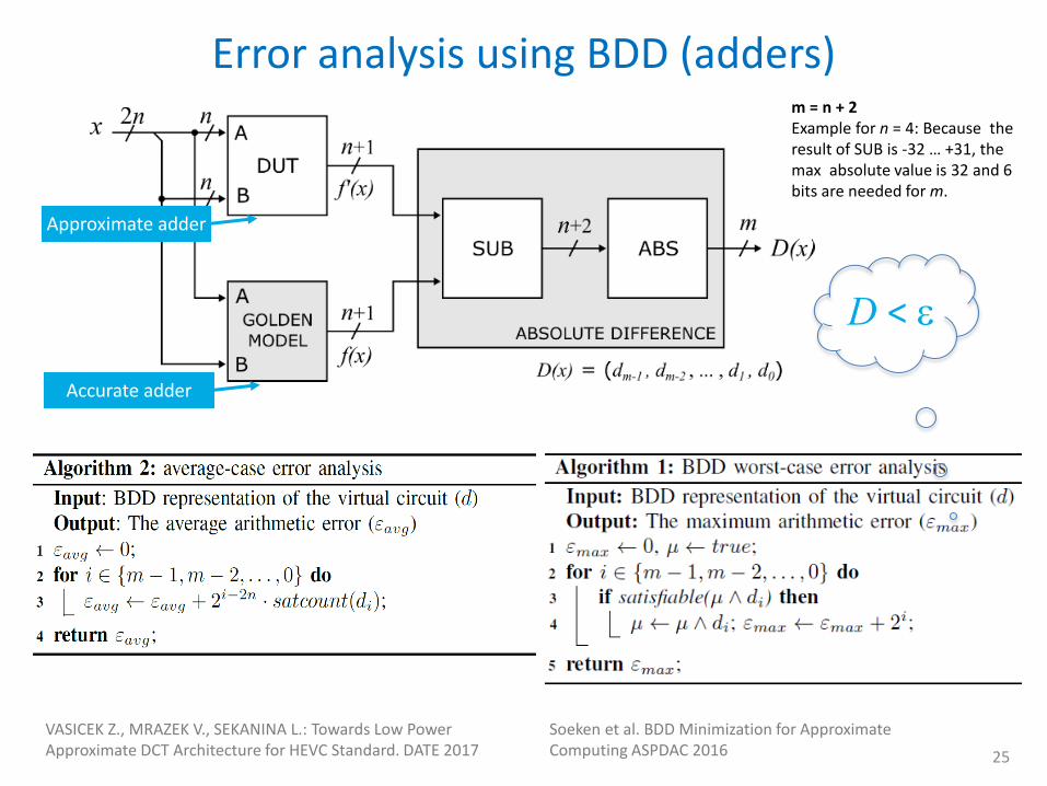
VASICEK Z., MRAZEK V., SEKANINA L.: Towards Low Power Approximate DCT Architecture for HEVC Standard. DATE 2017
Approximate adder
Accurate adder
m = n + 2 Example for n = 4: Because the result of SUB is -32 … +31, the max absolute value is 32 and 6 bits are needed for m.
Soeken et al. BDD Minimization for Approximate Computing ASPDAC 2016
D < e
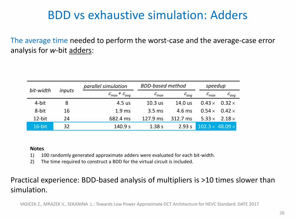
The average time needed to perform the worst-case and the average-case error analysis for w-bit adders:
Practical experience: BDD-based analysis of multipliers is >10 times slower than simulation.
BDD vs exhaustive simulation: Adders
26
bit-width inputs parallel simulation BDD-based method speedup
emax + eavg emax eavg emax eavg
4-bit 8 4.5 us 10.3 us 14.0 us 0.43 0.32
8-bit 16 1.9 ms 3.5 ms 4.6 ms 0.54 0.42
12-bit 24 682.4 ms 127.9 ms 312.7 ms 5.33 2.18
16-bit 32 140.9 s 1.38 s 2.93 s 102.3 48.09
Notes 1) 100 randomly generated approximate adders were evaluated for each bit-width. 2) The time required to construct a BDD for the virtual circuit is included.
VASICEK Z., MRAZEK V., SEKANINA L.: Towards Low Power Approximate DCT Architecture for HEVC Standard. DATE 2017
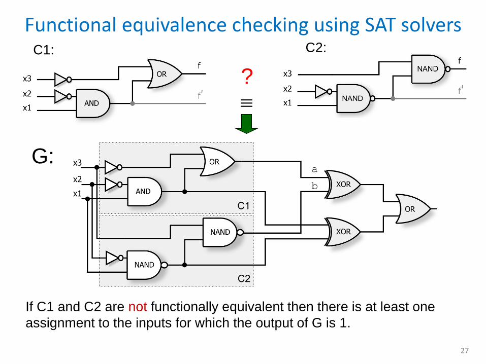
Functional equivalence checking using SAT solvers
27
?
If C1 and C2 are not functionally equivalent then there is at least one
assignment to the inputs for which the output of G is 1.
G:
C1: C2:
a
b
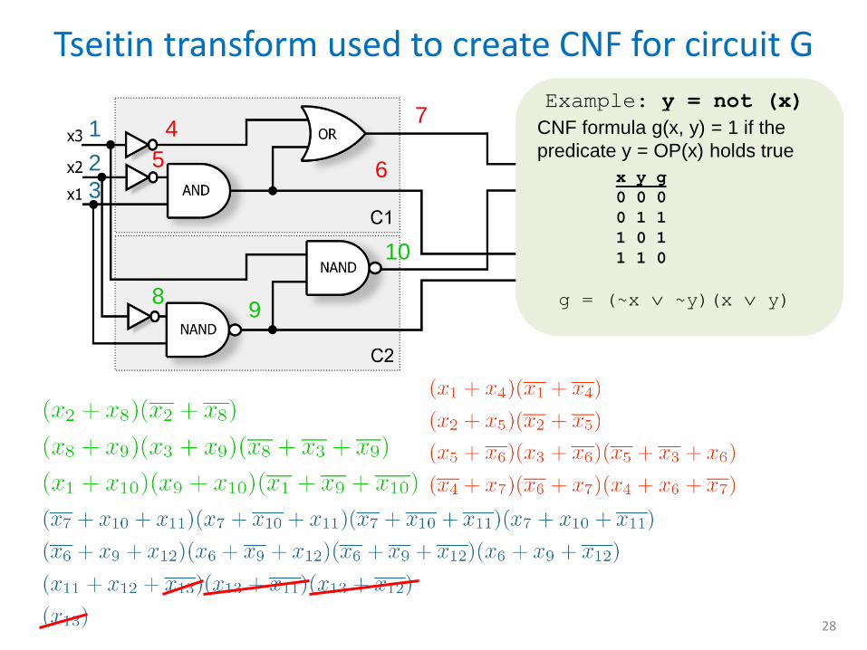
Tseitin transform used to create CNF for circuit G
28
7
6
1
2
3
4
5
8 9
10
11
12
13
Example: y = not (x)
x y g
0 0 0
0 1 1
1 0 1
1 1 0
g = (~x ~y)(x y)
CNF formula g(x, y) = 1 if the
predicate y = OP(x) holds true
SAT solver in action
29
7
6
1
2
3
4
5
8 9
10
11
12
13
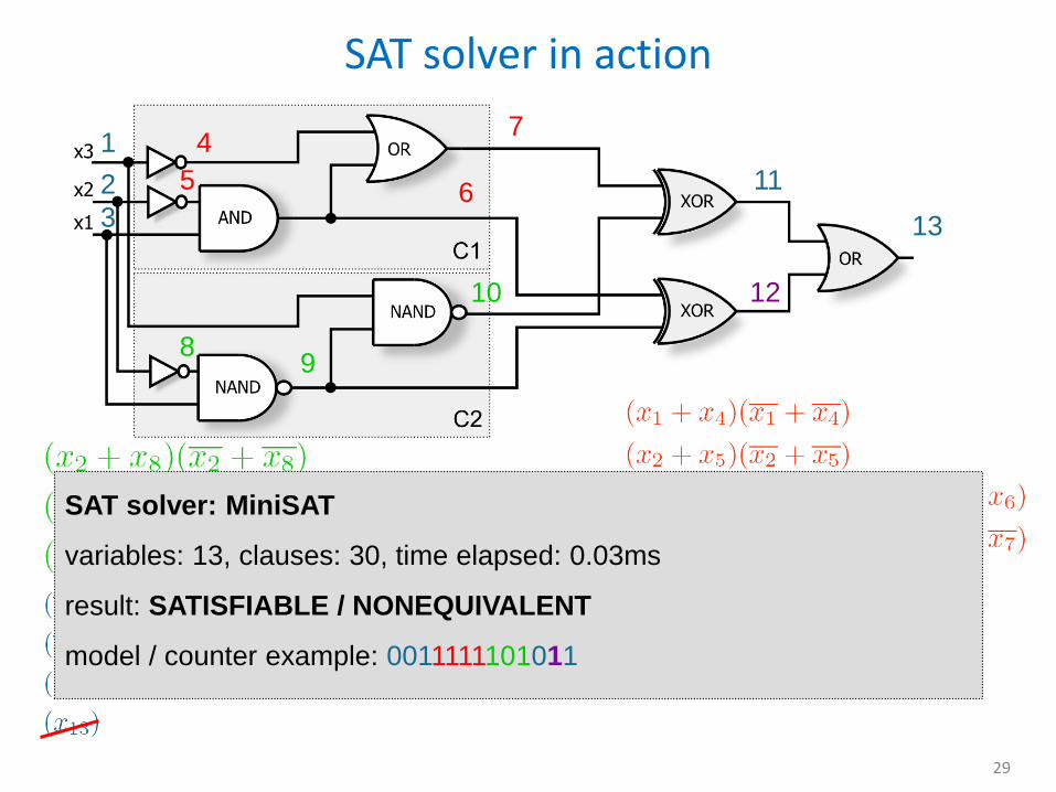
SAT solver: MiniSAT
variables: 13, clauses: 30, time elapsed: 0.03ms
result: SATISFIABLE / NONEQUIVALENT
model / counter example: 0011111101011
Worst-case error analysis using SAT solver
30
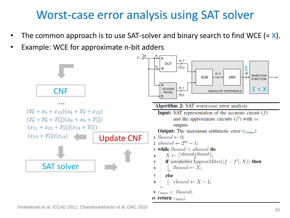
• The common approach is to use SAT-solver and binary search to find WCE (= X).
• Example: WCE for approximate n-bit adders
E < X
E
Venkatesan et al. ICCAD 2011; Chandrasekharan et al. DAC 2016
SAT solver
… CNF
Update CNF
On a fair comparison of automated approx. methods
31
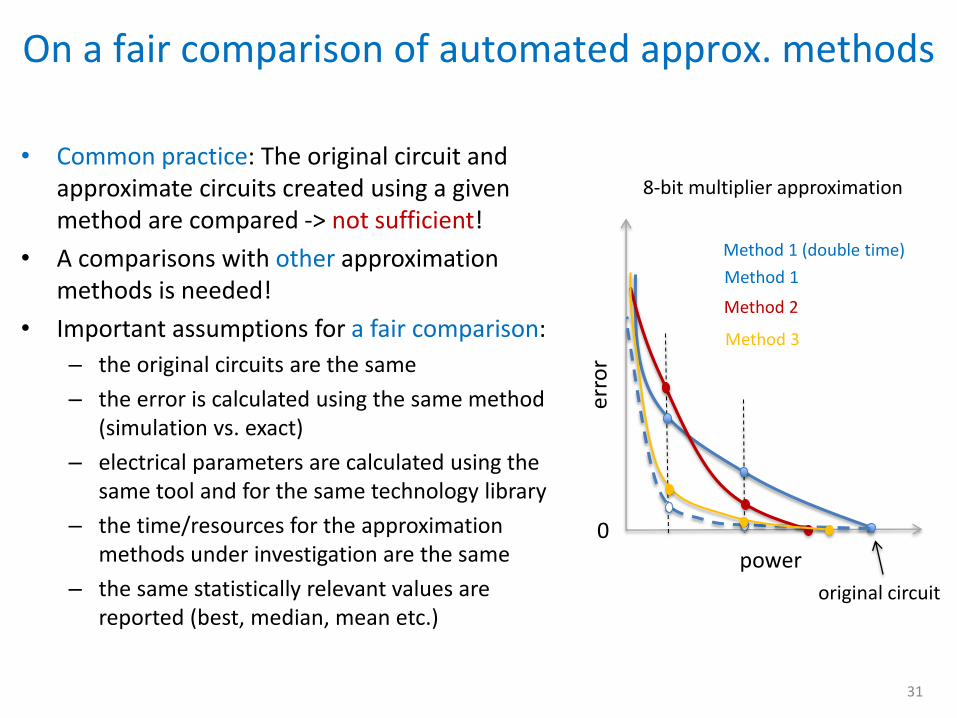
• Common practice: The original circuit and approximate circuits created using a given method are compared -> not sufficient!
• A comparisons with other approximation methods is needed!
• Important assumptions for a fair comparison:
– the original circuits are the same
– the error is calculated using the same method (simulation vs. exact)
– electrical parameters are calculated using the same tool and for the same technology library
– the time/resources for the approximation methods under investigation are the same
– the same statistically relevant values are reported (best, median, mean etc.)
8-bit multiplier approximation
power
erro
r
0
Method 1 (double time)
Method 1
Method 2
Method 3
original circuit
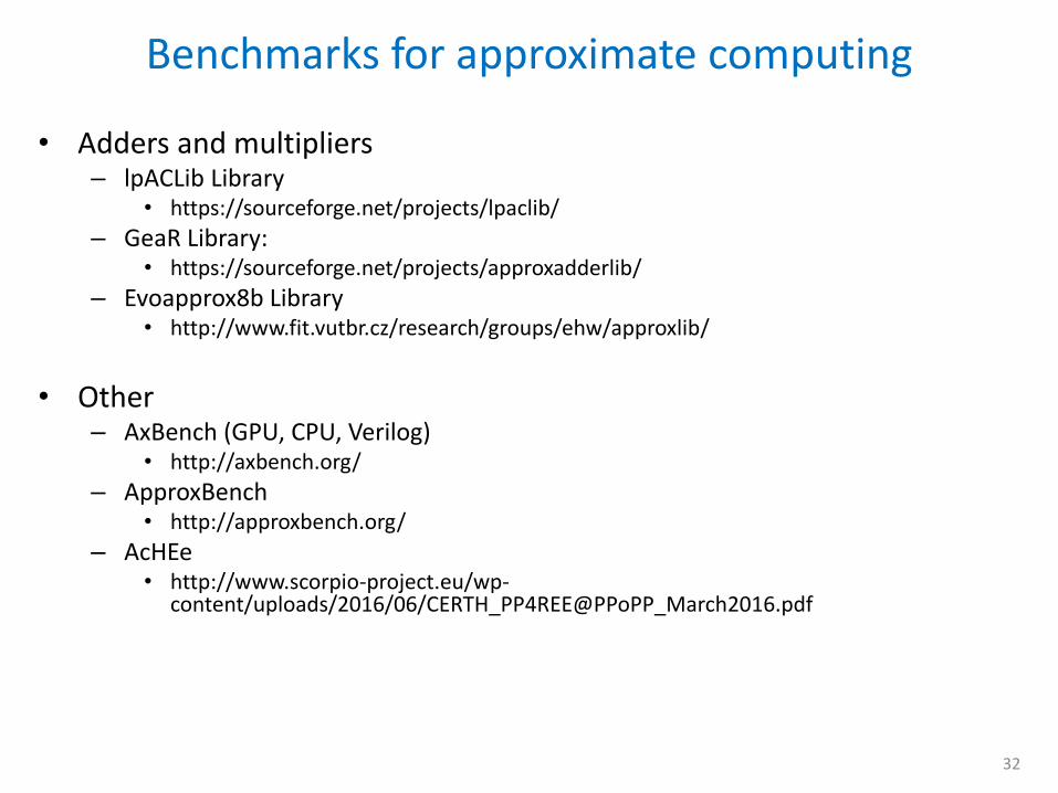
• Adders and multipliers – lpACLib Library
• https://sourceforge.net/projects/lpaclib/
– GeaR Library: • https://sourceforge.net/projects/approxadderlib/
– Evoapprox8b Library • http://www.fit.vutbr.cz/research/groups/ehw/approxlib/
• Other – AxBench (GPU, CPU, Verilog)
• http://axbench.org/
– ApproxBench • http://approxbench.org/
– AcHEe • http://www.scorpio-project.eu/wp-
content/uploads/2016/06/CERTH_PP4REE@PPoPP_March2016.pdf
Benchmarks for approximate computing
32
• Introduction • Design automation methods for approximate circuits
– Classification and overview – Circuit parameter estimation – Error computation – Relaxed equivalence checking – Evaluation methodology
• Examples of design automation methods for approximate circuits – Minterm complements, SASIMI, AIG rewriting, ABACUS, GRATER
• Evolutionary algorithms, CGP and circuit optimization • Applications of CGP-based approximation methods
– Open-source library of approximate adders and multipliers – Approximate TMR – Approximate multipliers in neural networks – Symbolic error analysis using BDDs/SAT solving in CGP-based tools – Approximate image filters
• Conclusions
Tutorial Outline – Part II.
33
Finding minterm complements to reduce # literals
34 Shin and Gupta: Approximate logic synthesis for error tolerant applications. DATE 2010 34
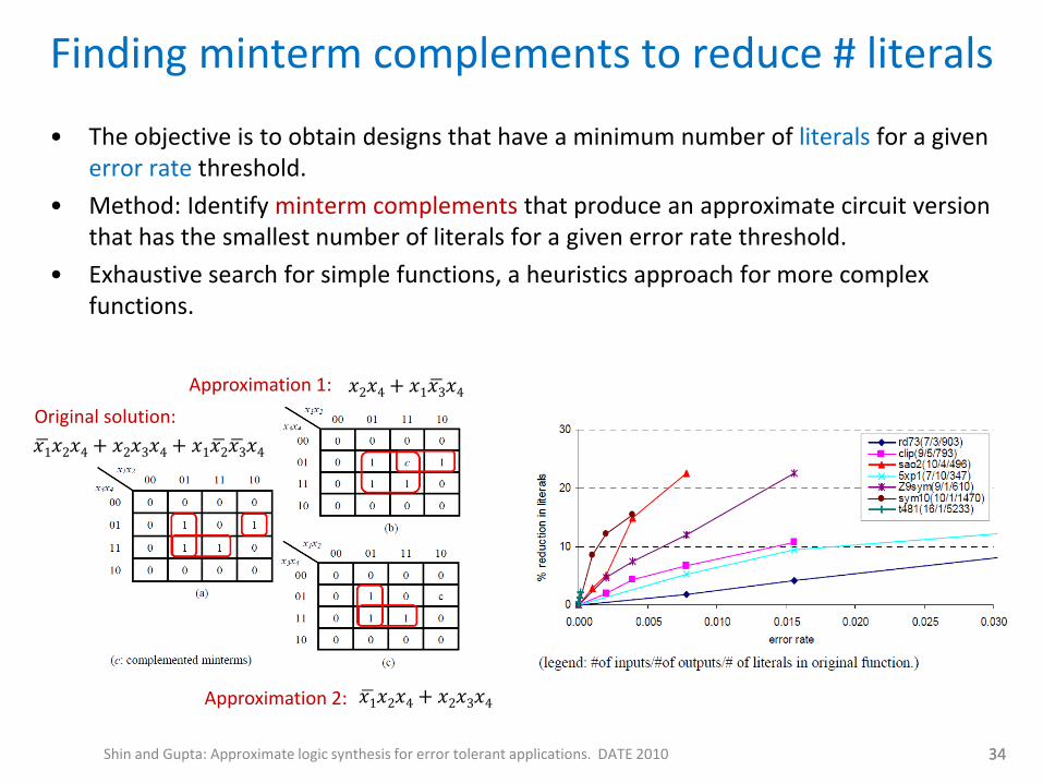
• The objective is to obtain designs that have a minimum number of literals for a given error rate threshold.
• Method: Identify minterm complements that produce an approximate circuit version that has the smallest number of literals for a given error rate threshold.
• Exhaustive search for simple functions, a heuristics approach for more complex functions.
𝑥1 𝑥2𝑥4 + 𝑥2𝑥3𝑥4 + 𝑥1𝑥2 𝑥3 𝑥4
𝑥2𝑥4 + 𝑥1𝑥3 𝑥4
𝑥1 𝑥2𝑥4 + 𝑥2𝑥3𝑥4
Original solution:
Approximation 1:
Approximation 2:
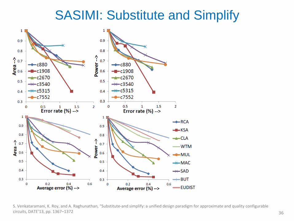
SASIMI: Substitute and Simplify
35
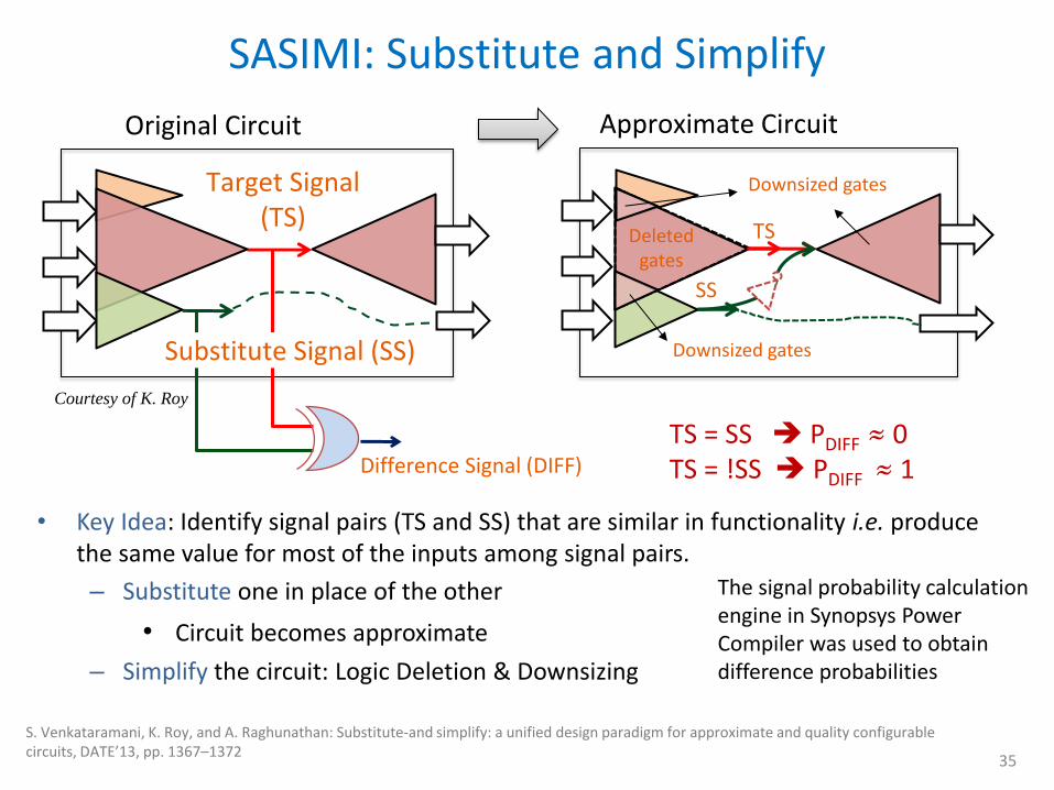
• Key Idea: Identify signal pairs (TS and SS) that are similar in functionality i.e. produce the same value for most of the inputs among signal pairs.
– Substitute one in place of the other
• Circuit becomes approximate
– Simplify the circuit: Logic Deletion & Downsizing
Original Circuit
TS = SS PDIFF ≈ 0 TS = !SS PDIFF ≈ 1 Difference Signal (DIFF)
Target Signal (TS)
Substitute Signal (SS)
Approximate Circuit
SS
Deleted gates
Downsized gates
Downsized gates
TS
S. Venkataramani, K. Roy, and A. Raghunathan: Substitute-and simplify: a unified design paradigm for approximate and quality configurable circuits, DATE’13, pp. 1367–1372
Courtesy of K. Roy
The signal probability calculation engine in Synopsys Power Compiler was used to obtain difference probabilities
SASIMI: Substitute and Simplify
36
S. Venkataramani, K. Roy, and A. Raghunathan, “Substitute-and simplify: a unified design paradigm for approximate and quality configurable circuits, DATE’13, pp. 1367–1372
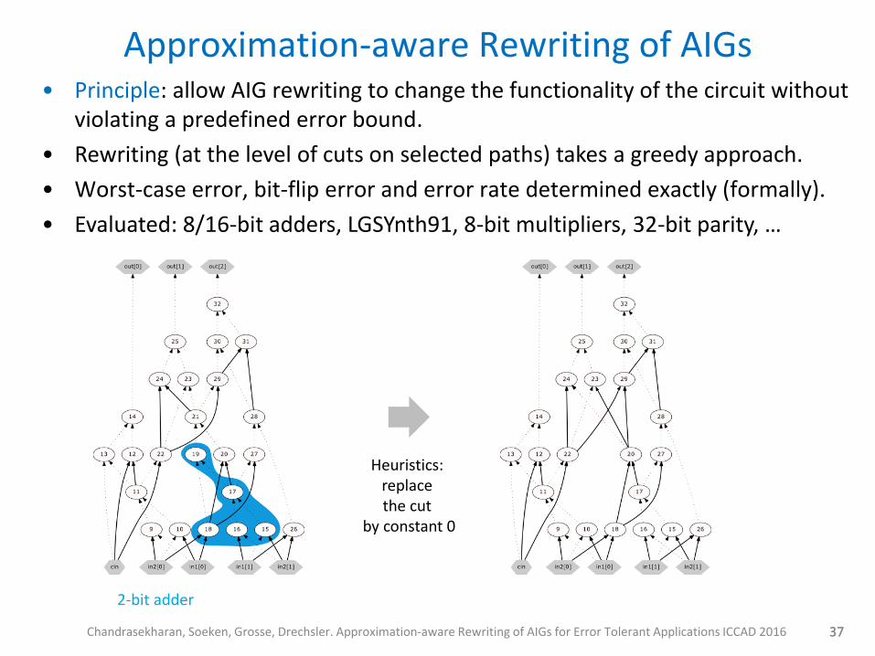
Approximation-aware Rewriting of AIGs
37 Chandrasekharan, Soeken, Grosse, Drechsler. Approximation-aware Rewriting of AIGs for Error Tolerant Applications ICCAD 2016 37
2-bit adder
Heuristics: replace the cut
by constant 0
• Principle: allow AIG rewriting to change the functionality of the circuit without violating a predefined error bound.
• Rewriting (at the level of cuts on selected paths) takes a greedy approach.
• Worst-case error, bit-flip error and error rate determined exactly (formally).
• Evaluated: 8/16-bit adders, LGSYnth91, 8-bit multipliers, 32-bit parity, …
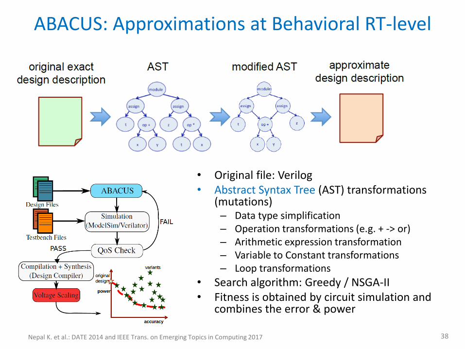
• Original file: Verilog • Abstract Syntax Tree (AST) transformations
(mutations) – Data type simplification – Operation transformations (e.g. + -> or) – Arithmetic expression transformation – Variable to Constant transformations – Loop transformations
• Search algorithm: Greedy / NSGA-II • Fitness is obtained by circuit simulation and
combines the error & power
ABACUS: Approximations at Behavioral RT-level
38 Nepal K. et al.: DATE 2014 and IEEE Trans. on Emerging Topics in Computing 2017
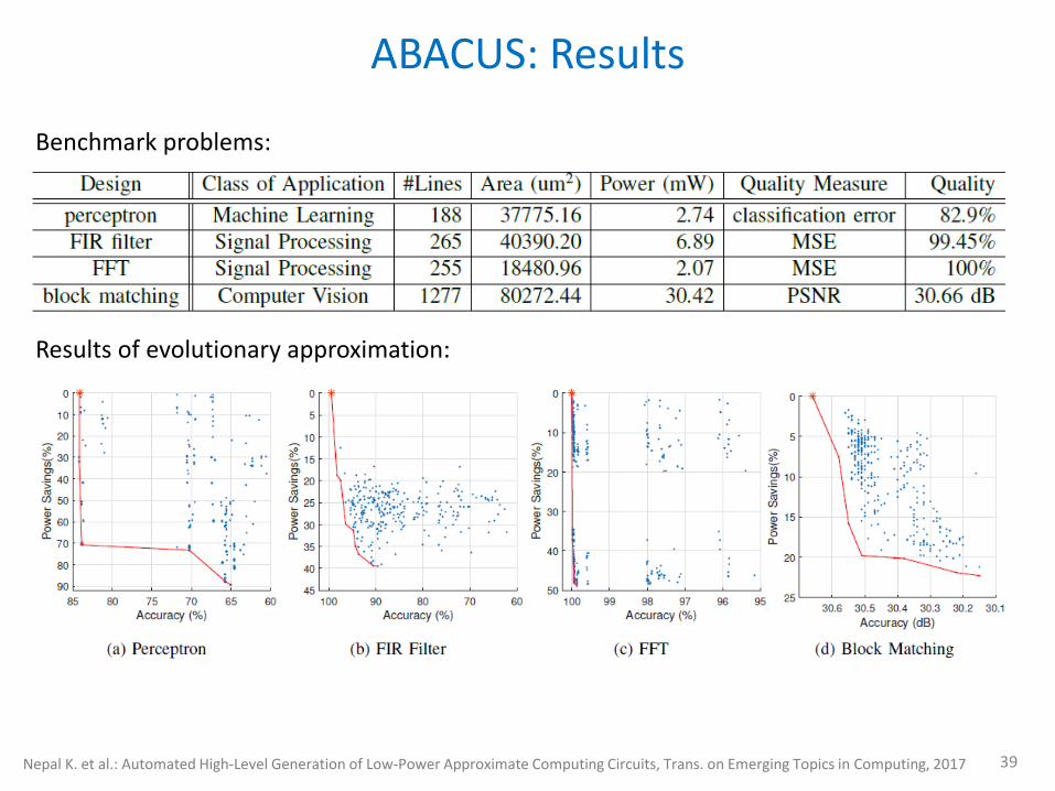
ABACUS: Results
39 Nepal K. et al.: Automated High-Level Generation of Low-Power Approximate Computing Circuits, Trans. on Emerging Topics in Computing, 2017
Benchmark problems:
Results of evolutionary approximation:
GRATER: GA-based optimization of data types
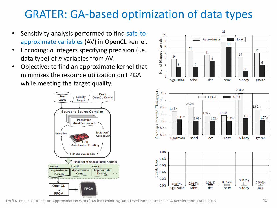
40 Lotfi A. et al.: GRATER: An Approximation Workflow for Exploiting Data-Level Parallelism in FPGA Acceleration. DATE 2016
• Sensitivity analysis performed to find safe-to-approximate variables (AV) in OpenCL kernel.
• Encoding: n integers specifying precision (i.e. data type) of n variables from AV.
• Objective: to find an approximate kernel that minimizes the resource utilization on FPGA while meeting the target quality.

• Introduction • Design automation methods for approximate circuits
– Classification and overview – Circuit parameter estimation – Error computation – Relaxed equivalence checking – Evaluation methodology
• Examples of design automation methods for approximate circuits – Minterm complements, SASIMI, AIG rewriting, ABACUS, GRATER
• Evolutionary algorithms, CGP and circuit optimization • Applications of CGP-based approximation methods
– Open-source library of approximate adders and multipliers – Approximate TMR – Approximate multipliers in neural networks – Symbolic error analysis using BDDs/SAT solving in CGP-based tools – Approximate image filters
• Conclusions
Tutorial Outline – Part II.
41
Evolutionary algorithms: GA, ES, EP, GP, LGP, CGP, …
42
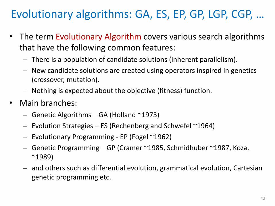
• The term Evolutionary Algorithm covers various search algorithms that have the following common features: – There is a population of candidate solutions (inherent parallelism).
– New candidate solutions are created using operators inspired in genetics (crossover, mutation).
– Nothing is expected about the objective (fitness) function.
• Main branches: – Genetic Algorithms – GA (Holland ~1973)
– Evolution Strategies – ES (Rechenberg and Schwefel ~1964)
– Evolutionary Programming - EP (Fogel ~1962)
– Genetic Programming – GP (Cramer ~1985, Schmidhuber ~1987, Koza, ~1989)
– and others such as differential evolution, grammatical evolution, Cartesian genetic programming etc.
Evolutionary algorithms: GA, GP, LGP, CGP, GE …
43
fitn
ess
chromosomes
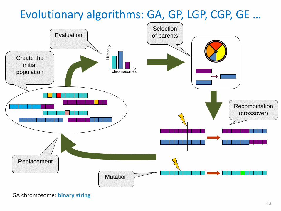
Create the
initial
population
Evaluation Selection
of parents
Recombination
(crossover)
Mutation
Replacement
GA chromosome: binary string
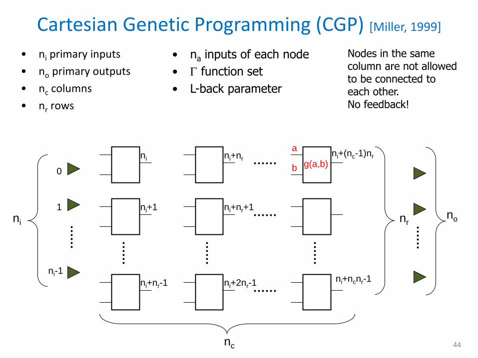
Cartesian Genetic Programming (CGP) [Miller, 1999]
44
• ni primary inputs
• no primary outputs
• nc columns
• nr rows
ni
ni+1
ni+nr-1
ni+nr
ni+nr+1
ni+2nr-1
ni+(nc-1)nr
• na inputs of each node
• function set
• L-back parameter
ni+ncnr-1
nr
nc
0
1
ni-1
ni no
Nodes in the same column are not allowed to be connected to each other. No feedback!
a
b g(a,b)
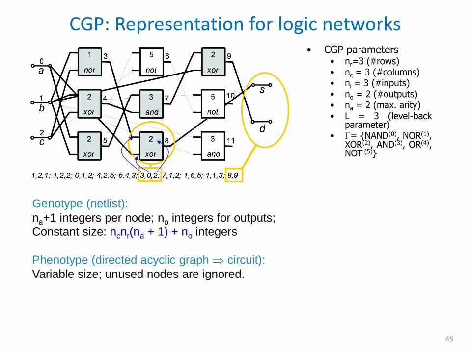
CGP: Representation for logic networks
45
Genotype (netlist):
na+1 integers per node; no integers for outputs;
Constant size: ncnr(na + 1) + no integers
Phenotype (directed acyclic graph circuit):
Variable size; unused nodes are ignored.
• CGP parameters • nr=3 (#rows) • nc = 3 (#columns) • ni = 3 (#inputs) • no = 2 (#outputs) • na = 2 (max. arity) • L = 3 (level-back
parameter) • = {NAND(0), NOR(1),
XOR(2), AND(3), OR(4), NOT (5)}
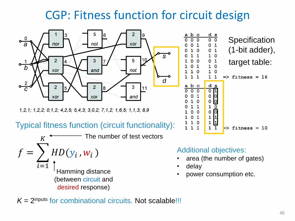
CGP: Fitness function for circuit design
46
target table:
Specification
(1-bit adder),
Typical fitness function (circuit functionality):
𝑓 = 𝐻𝐷(𝑦𝑖
𝐾
𝑖=1
, 𝑤𝑖 )
Hamming distance
(between circuit and
desired response)
The number of test vectors
K = 2inputs for combinational circuits. Not scalable!!!
Additional objectives: • area (the number of gates)
• delay
• power consumption etc.
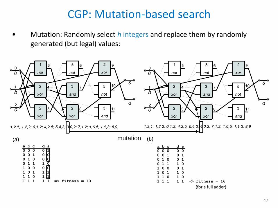
CGP: Mutation-based search
47
mutation
• Mutation: Randomly select h integers and replace them by randomly generated (but legal) values:
(for a full adder)
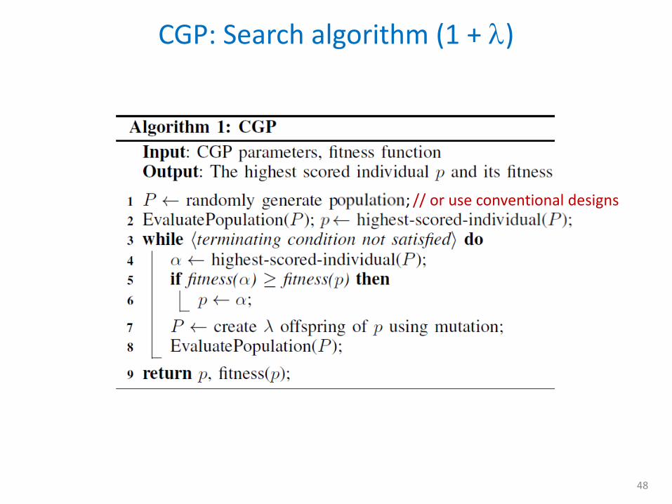
CGP: Search algorithm (1 + )
48
; // or use conventional designs
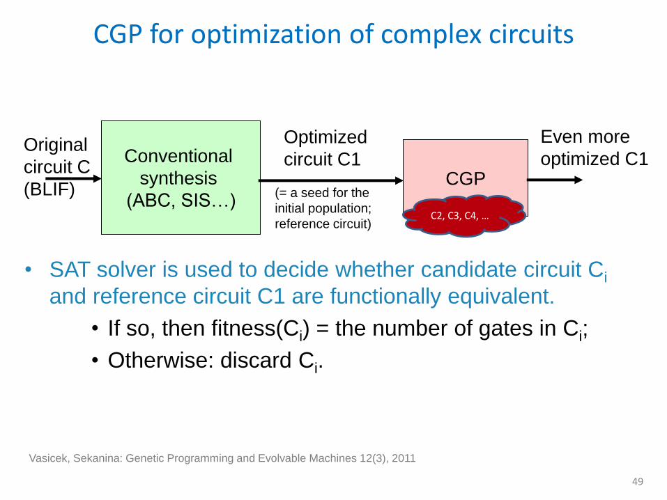
CGP for optimization of complex circuits
49
• SAT solver is used to decide whether candidate circuit Ci
and reference circuit C1 are functionally equivalent.
• If so, then fitness(Ci) = the number of gates in Ci;
• Otherwise: discard Ci.
Conventional
synthesis
(ABC, SIS…) CGP
Optimized
circuit C1
Even more
optimized C1
(= a seed for the
initial population;
reference circuit)
Vasicek, Sekanina: Genetic Programming and Evolvable Machines 12(3), 2011
Original
circuit C
(BLIF)
C2, C3, C4, …
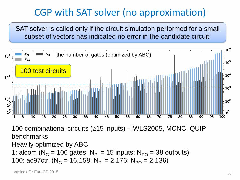
CGP with SAT solver (no approximation)
50
SAT solver is called only if the circuit simulation performed for a small subset of vectors has indicated no error in the candidate circuit.
100 combinational circuits (15 inputs) - IWLS2005, MCNC, QUIP
benchmarks
Heavily optimized by ABC
1: alcom (NG = 106 gates; NPI = 15 inputs; NPO = 38 outputs)
100: ac97ctrl (NG = 16,158; NPI = 2,176; NPO = 2,136)
- the number of gates (optimized by ABC)
100 test circuits
Vasicek Z.: EuroGP 2015
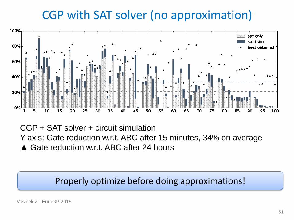
CGP with SAT solver (no approximation)
51
CGP + SAT solver + circuit simulation
Y-axis: Gate reduction w.r.t. ABC after 15 minutes, 34% on average
▲ Gate reduction w.r.t. ABC after 24 hours
Vasicek Z.: EuroGP 2015
Properly optimize before doing approximations!
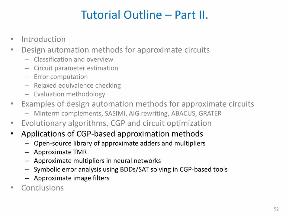
• Introduction • Design automation methods for approximate circuits
– Classification and overview – Circuit parameter estimation – Error computation – Relaxed equivalence checking – Evaluation methodology
• Examples of design automation methods for approximate circuits – Minterm complements, SASIMI, AIG rewriting, ABACUS, GRATER
• Evolutionary algorithms, CGP and circuit optimization • Applications of CGP-based approximation methods
– Open-source library of approximate adders and multipliers – Approximate TMR – Approximate multipliers in neural networks – Symbolic error analysis using BDDs/SAT solving in CGP-based tools – Approximate image filters
• Conclusions
Tutorial Outline – Part II.
52
• In approximate computing, partially working solutions are sought.
• In EA, partially working solutions are improved.
• EAs are excellent in multi-objective design and optimization.
• Constraints can easily be handled.
• EA can be seeded with the original code (circuit).
• EA is easy to implement and parallelize.
Why EA in approximate computing?
53
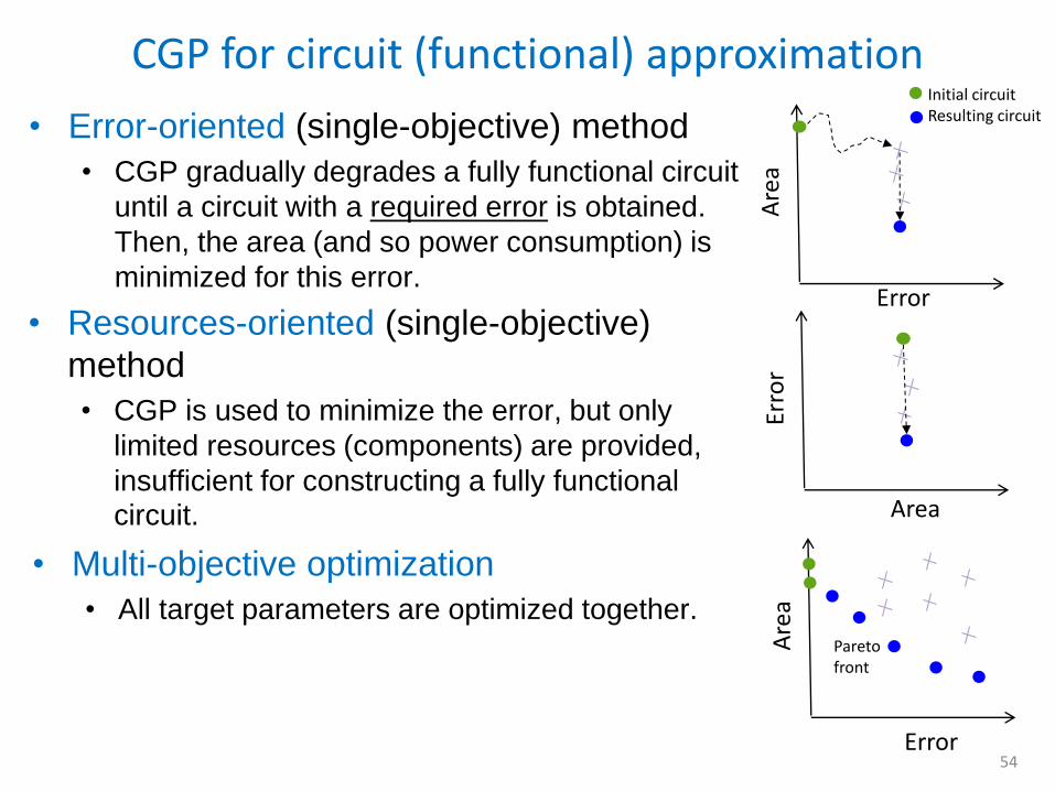
CGP for circuit (functional) approximation
54
• Error-oriented (single-objective) method
• CGP gradually degrades a fully functional circuit
until a circuit with a required error is obtained.
Then, the area (and so power consumption) is
minimized for this error. Error
Are
a
Area
Erro
r
• Resources-oriented (single-objective)
method
• CGP is used to minimize the error, but only
limited resources (components) are provided,
insufficient for constructing a fully functional circuit.
Are
a
Pareto front
Error
• Multi-objective optimization
• All target parameters are optimized together.
Initial circuit Resulting circuit
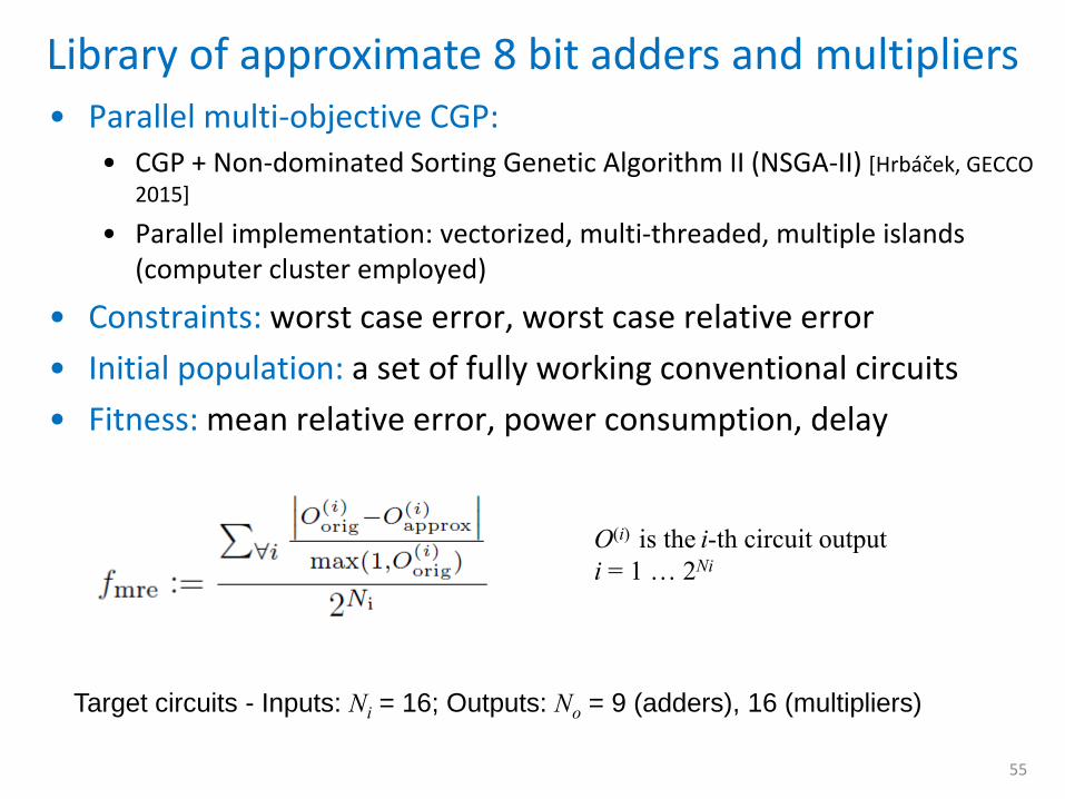
Library of approximate 8 bit adders and multipliers
55
• Parallel multi-objective CGP: • CGP + Non-dominated Sorting Genetic Algorithm II (NSGA-II) [Hrbáček, GECCO
2015]
• Parallel implementation: vectorized, multi-threaded, multiple islands (computer cluster employed)
• Constraints: worst case error, worst case relative error
• Initial population: a set of fully working conventional circuits
• Fitness: mean relative error, power consumption, delay
Target circuits - Inputs: Ni = 16; Outputs: No = 9 (adders), 16 (multipliers)
O(i) is the i-th circuit output
i = 1 … 2Ni
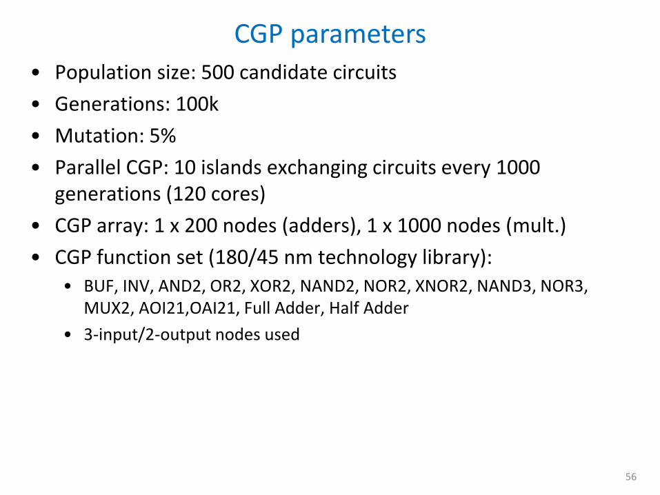
CGP parameters
56
• Population size: 500 candidate circuits
• Generations: 100k
• Mutation: 5%
• Parallel CGP: 10 islands exchanging circuits every 1000 generations (120 cores)
• CGP array: 1 x 200 nodes (adders), 1 x 1000 nodes (mult.)
• CGP function set (180/45 nm technology library):
• BUF, INV, AND2, OR2, XOR2, NAND2, NOR2, XNOR2, NAND3, NOR3, MUX2, AOI21,OAI21, Full Adder, Half Adder
• 3-input/2-output nodes used
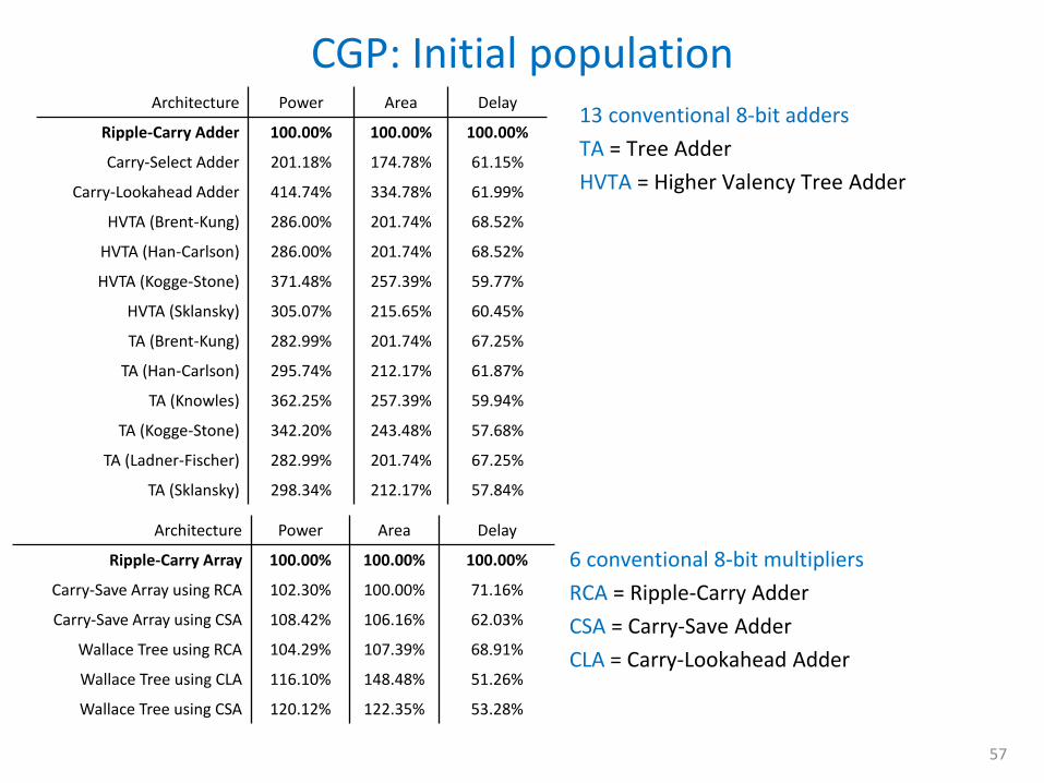
CGP: Initial population
57
Architecture Power Area Delay
Ripple-Carry Adder 100.00% 100.00% 100.00%
Carry-Select Adder 201.18% 174.78% 61.15%
Carry-Lookahead Adder 414.74% 334.78% 61.99%
HVTA (Brent-Kung) 286.00% 201.74% 68.52%
HVTA (Han-Carlson) 286.00% 201.74% 68.52%
HVTA (Kogge-Stone) 371.48% 257.39% 59.77%
HVTA (Sklansky) 305.07% 215.65% 60.45%
TA (Brent-Kung) 282.99% 201.74% 67.25%
TA (Han-Carlson) 295.74% 212.17% 61.87%
TA (Knowles) 362.25% 257.39% 59.94%
TA (Kogge-Stone) 342.20% 243.48% 57.68%
TA (Ladner-Fischer) 282.99% 201.74% 67.25%
TA (Sklansky) 298.34% 212.17% 57.84%
13 conventional 8-bit adders
TA = Tree Adder
HVTA = Higher Valency Tree Adder
Architecture Power Area Delay
Ripple-Carry Array 100.00% 100.00% 100.00%
Carry-Save Array using RCA 102.30% 100.00% 71.16%
Carry-Save Array using CSA 108.42% 106.16% 62.03%
Wallace Tree using RCA 104.29% 107.39% 68.91%
Wallace Tree using CLA 116.10% 148.48% 51.26%
Wallace Tree using CSA 120.12% 122.35% 53.28%
6 conventional 8-bit multipliers
RCA = Ripple-Carry Adder
CSA = Carry-Save Adder
CLA = Carry-Lookahead Adder
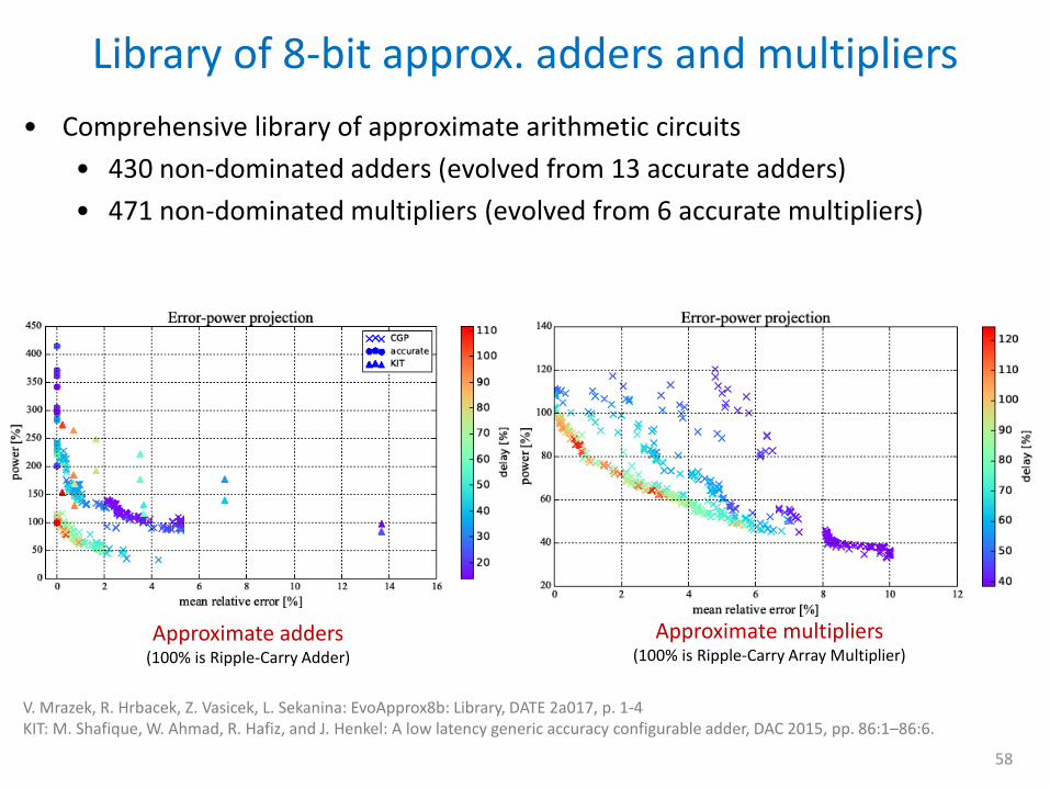
Library of 8-bit approx. adders and multipliers
58
• Comprehensive library of approximate arithmetic circuits
• 430 non-dominated adders (evolved from 13 accurate adders)
• 471 non-dominated multipliers (evolved from 6 accurate multipliers)
V. Mrazek, R. Hrbacek, Z. Vasicek, L. Sekanina: EvoApprox8b: Library, DATE 2a017, p. 1-4 KIT: M. Shafique, W. Ahmad, R. Hafiz, and J. Henkel: A low latency generic accuracy configurable adder, DAC 2015, pp. 86:1–86:6.
Approximate adders (100% is Ripple-Carry Adder)
Approximate multipliers (100% is Ripple-Carry Array Multiplier)
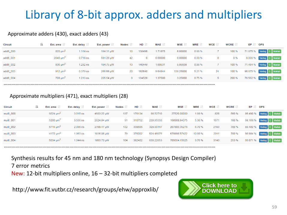
Library of 8-bit approx. adders and multipliers
59
http://www.fit.vutbr.cz/research/groups/ehw/approxlib/
Approximate adders (430), exact adders (43)
Approximate multipliers (471), exact multipliers (28)
…………………………………………………………………………………………………………………………………………………
…………………………………………………………………………………………………………………………………………………
Synthesis results for 45 nm and 180 nm technology (Synopsys Design Compiler) 7 error metrics New: 12-bit multipliers online, 16 – 32-bit multipliers completed
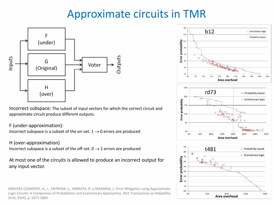
Approximate circuits in TMR
60
b12
rd73
t481
SÁNCHEZ-CLEMENTE, A., J., ENTRENA, L., HRBACEK, R. a SEKANINA, L. Error Mitigation using Approximate Logic Circuits: A Comparison of Probabilistic and Evolutionary Approaches. IEEE Transactions on Reliability. 2016, 65(4), p. 1871-1883
Incorrect subspace: The subset of input vectors for which the correct circuit and approximate circuit produce different outputs.
F (under-approximation): Incorrect subspace is a subset of the on-set. 1 0 errors are produced
H (over-approximation) Incorrect subspace is a subset of the off-set. 0 1 errors are produced
At most one of the circuits is allowed to produce an incorrect output for any input vector.
Energy-efficient implementation of ANNs
61
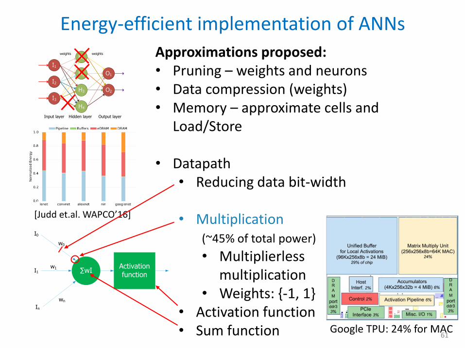
Approximations proposed: • Pruning – weights and neurons • Data compression (weights) • Memory – approximate cells and
Load/Store
• Datapath • Reducing data bit-width
• Multiplication (~45% of total power)
• Multiplierless multiplication
• Weights: {-1, 1} • Activation function • Sum function
[Judd et.al. WAPCO’16]
∑wI
I0
I1
In
w0
w1
wn
Activation function
H1
H2
H3
H4
I1
I2
I3
O1
O2
Hidden layerInput layer Output layer
weights weights
Google TPU: 24% for MAC
Energy-efficient implementation of ANNs
62
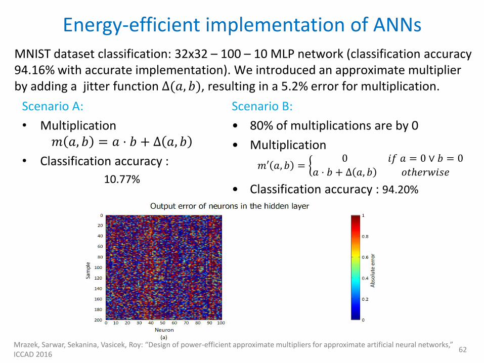
Scenario A:
• Multiplication 𝑚 𝑎, 𝑏 = 𝑎 ⋅ 𝑏 + Δ 𝑎, 𝑏
• Classification accuracy :
10.77%
MNIST dataset classification: 32x32 – 100 – 10 MLP network (classification accuracy 94.16% with accurate implementation). We introduced an approximate multiplier by adding a jitter function Δ(𝑎, 𝑏), resulting in a 5.2% error for multiplication.
Scenario B:
• 80% of multiplications are by 0
• Multiplication
𝑚′ 𝑎, 𝑏 = 0 𝑖𝑓 𝑎 = 0 ∨ 𝑏 = 0
𝑎 ⋅ 𝑏 + Δ 𝑎, 𝑏 𝑜𝑡ℎ𝑒𝑟𝑤𝑖𝑠𝑒
• Classification accuracy : 94.20%
Mrazek, Sarwar, Sekanina, Vasicek, Roy: “Design of power-efficient approximate multipliers for approximate artificial neural networks,” ICCAD 2016
CGP in approx. multiplier design for ANNs
63 Mrazek, Sarwar, Sekanina, Vasicek, Roy: “Design of power-efficient approximate multipliers for approximate artificial neural networks,” ICCAD 2016
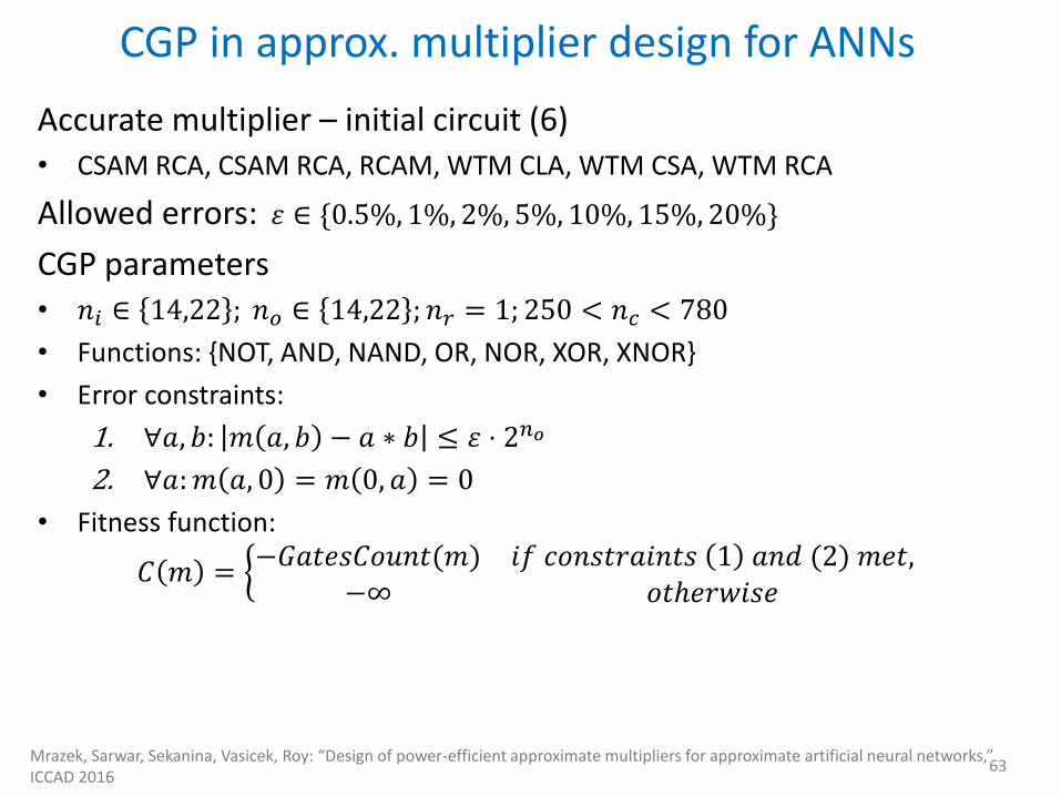
Accurate multiplier – initial circuit (6) • CSAM RCA, CSAM RCA, RCAM, WTM CLA, WTM CSA, WTM RCA
Allowed errors: 𝜀 ∈ {0.5%, 1%, 2%, 5%, 10%, 15%, 20%}
CGP parameters • 𝑛𝑖 ∈ 14,22 ; 𝑛𝑜 ∈ 14,22 ; 𝑛𝑟 = 1; 250 < 𝑛𝑐 < 780
• Functions: {NOT, AND, NAND, OR, NOR, XOR, XNOR}
• Error constraints:
1. ∀𝑎, 𝑏: 𝑚 𝑎, 𝑏 − 𝑎 ∗ 𝑏 ≤ 𝜀 ⋅ 2𝑛𝑜
2. ∀𝑎: 𝑚 𝑎, 0 = 𝑚 0, 𝑎 = 0
• Fitness function:
𝐶 𝑚 = −𝐺𝑎𝑡𝑒𝑠𝐶𝑜𝑢𝑛𝑡(𝑚) 𝑖𝑓 𝑐𝑜𝑛𝑠𝑡𝑟𝑎𝑖𝑛𝑡𝑠 1 𝑎𝑛𝑑 (2) 𝑚𝑒𝑡,
−∞ 𝑜𝑡ℎ𝑒𝑟𝑤𝑖𝑠𝑒
CGP in approx. multiplier design for ANNs
64 Mrazek, Sarwar, Sekanina, Vasicek, Roy: “Design of power-efficient approximate multipliers for approximate artificial neural networks,” ICCAD 2016
• In total, 852 approximate 7-bit and 11-bit multipliers were evolved by CGP.
• Multipliers were sign-extended using one’s complement.
• The 8-bit and 12-bit multipliers were applied in NNs.
• The NNs were retrained with approximate multiplication operation using the backpropagation algorithm.
• Approximate multipliers showing the best trade off between power and accuracy in NN were selected (for different error targets).
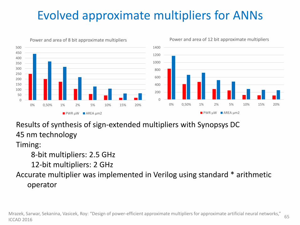
Evolved approximate multipliers for ANNs
65
0
50
100
150
200
250
300
350
400
450
500
0% 0,50% 1% 2% 5% 10% 15% 20%
Power and area of 8 bit approximate multipliers
PWR μW AREA μm2
0
200
400
600
800
1000
1200
1400
0% 0,50% 1% 2% 5% 10% 15% 20%
Power and area of 12 bit approximate multipliers
PWR μW AREA μm2
Results of synthesis of sign-extended multipliers with Synopsys DC 45 nm technology Timing:
8-bit multipliers: 2.5 GHz 12-bit multipliers: 2 GHz
Accurate multiplier was implemented in Verilog using standard * arithmetic operator
Mrazek, Sarwar, Sekanina, Vasicek, Roy: “Design of power-efficient approximate multipliers for approximate artificial neural networks,” ICCAD 2016
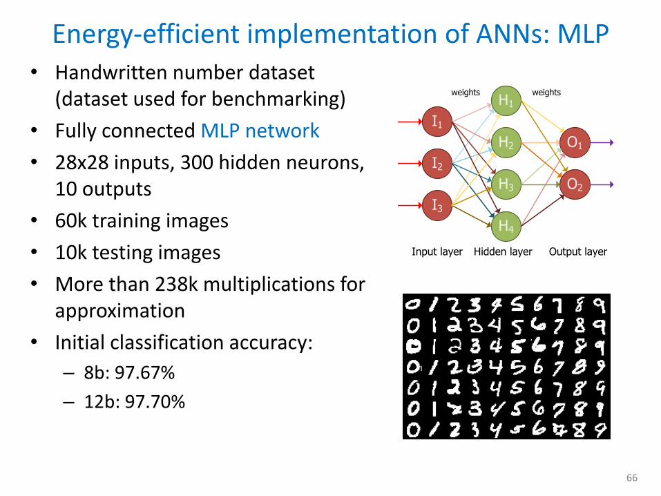
Energy-efficient implementation of ANNs: MLP
66
• Handwritten number dataset (dataset used for benchmarking)
• Fully connected MLP network
• 28x28 inputs, 300 hidden neurons, 10 outputs
• 60k training images
• 10k testing images
• More than 238k multiplications for approximation
• Initial classification accuracy:
– 8b: 97.67%
– 12b: 97.70%
H1
H2
H3
H4
I1
I2
I3
O1
O2
Hidden layerInput layer Output layer
weights weights
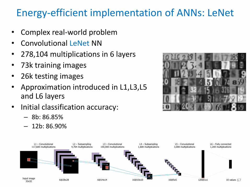
Energy-efficient implementation of ANNs: LeNet
67
• Complex real-world problem
• Convolutional LeNet NN
• 278,104 multiplications in 6 layers
• 73k training images
• 26k testing images
• Approximation introduced in L1,L3,L5 and L6 layers
• Initial classification accuracy: – 8b: 86.85%
– 12b: 86.90%
Input image32x32
6@28x28 6@14x14 16@10x10 16@5x5 120@1x1 10 values
L1 – Convolutional117,600 multiplications
L2 – Subsampling4,704 multiplications
L3 – Convolutional150,000 multiplications
L4 – Subsampling1,600 multiplications
L5 – Convolutional3,000 multiplications
L6 – Fully connected1,200 multiplications
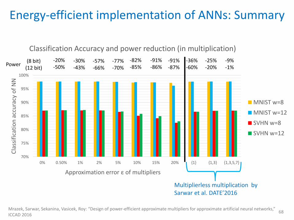
Energy-efficient implementation of ANNs: Summary
68 Mrazek, Sarwar, Sekanina, Vasicek, Roy: “Design of power-efficient approximate multipliers for approximate artificial neural networks,” ICCAD 2016
-9% -1%
-25% -20%
-36% -60%
70%
75%
80%
85%
90%
95%
100%
0% 0.50% 1% 2% 5% 10% 15% 20% {1} {1,3} {1,3,5,7}
Cla
ssif
icat
ion
acc
ura
cy o
f N
N
Approximation error ε of multipliers
Classification Accuracy and power reduction (in multiplication)
MNIST w=8
MNIST w=12
SVHN w=8
SVHN w=12
Multiplierless multiplication by Sarwar et al. DATE’2016
-20% -50%
-30% -43%
(8 bit) (12 bit)
Power -57% -66%
-77% -70%
-82% -85%
-91% -86%
-91% -87%
Circuit approximation with CGP and BDD
69
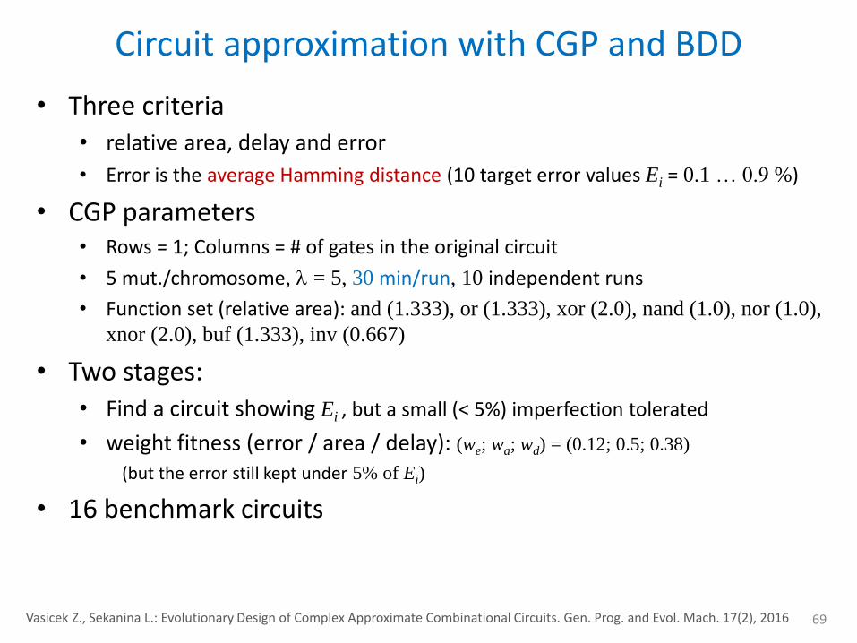
• Three criteria • relative area, delay and error
• Error is the average Hamming distance (10 target error values Ei = 0.1 … 0.9 %)
• CGP parameters • Rows = 1; Columns = # of gates in the original circuit
• 5 mut./chromosome, = 5, 30 min/run, 10 independent runs
• Function set (relative area): and (1.333), or (1.333), xor (2.0), nand (1.0), nor (1.0),
xnor (2.0), buf (1.333), inv (0.667)
• Two stages: • Find a circuit showing Ei , but a small (< 5%) imperfection tolerated
• weight fitness (error / area / delay): (we; wa; wd) = (0.12; 0.5; 0.38)
(but the error still kept under 5% of Ei)
• 16 benchmark circuits
Vasicek Z., Sekanina L.: Evolutionary Design of Complex Approximate Combinational Circuits. Gen. Prog. and Evol. Mach. 17(2), 2016
Hamming distance using BDDs
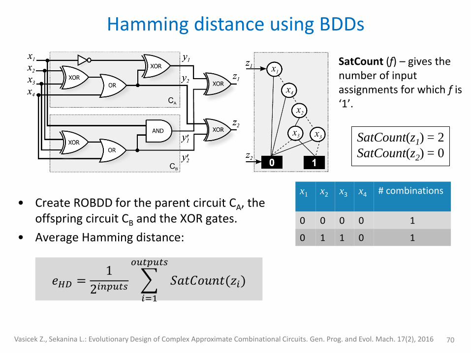
70
• Create ROBDD for the parent circuit CA, the offspring circuit CB and the XOR gates.
• Average Hamming distance:
SatCount(z1) = 2
SatCount(z2) = 0
SatCount (f) – gives the number of input assignments for which f is ‘1’.
x1 x2 x3 x4 # combinations
0 0 0 0 1
0 1 1 0 1
𝑒𝐻𝐷 =1
2𝑖𝑛𝑝𝑢𝑡𝑠 𝑆𝑎𝑡𝐶𝑜𝑢𝑛𝑡(𝑧𝑖)
𝑜𝑢𝑡𝑝𝑢𝑡𝑠
𝑖=1
Vasicek Z., Sekanina L.: Evolutionary Design of Complex Approximate Combinational Circuits. Gen. Prog. and Evol. Mach. 17(2), 2016
CGP with BDD in the fitness function: Example 1
71
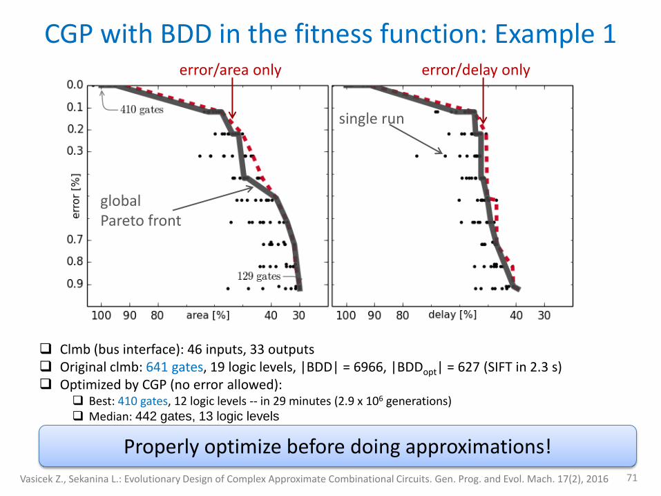
error/delay only
single run
error/area only
global Pareto front
Properly optimize before doing approximations!
Clmb (bus interface): 46 inputs, 33 outputs Original clmb: 641 gates, 19 logic levels, |BDD| = 6966, |BDDopt| = 627 (SIFT in 2.3 s) Optimized by CGP (no error allowed):
Best: 410 gates, 12 logic levels -- in 29 minutes (2.9 x 10⁶ generations) Median: 442 gates, 13 logic levels
Vasicek Z., Sekanina L.: Evolutionary Design of Complex Approximate Combinational Circuits. Gen. Prog. and Evol. Mach. 17(2), 2016
CGP with BDD in the fitness function: Example 2
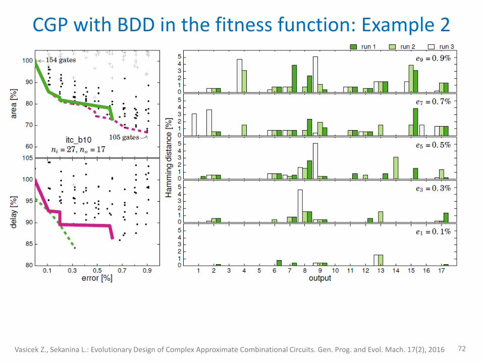
72 Vasicek Z., Sekanina L.: Evolutionary Design of Complex Approximate Combinational Circuits. Gen. Prog. and Evol. Mach. 17(2), 2016
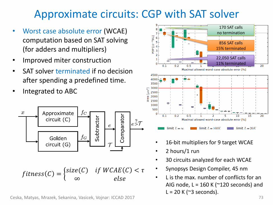
Approximate circuits: CGP with SAT solver
73 Ceska, Matyas, Mrazek, Sekanina, Vasicek, Vojnar: ICCAD 2017
• Worst case absolute error (WCAE) computation based on SAT solving (for adders and multipliers)
• Improved miter construction
• SAT solver terminated if no decision after spending a predefined time.
• Integrated to ABC
𝑓𝑖𝑡𝑛𝑒𝑠𝑠 𝐶 = 𝑠𝑖𝑧𝑒(𝐶) 𝑖𝑓 𝑊𝐶𝐴𝐸 𝐶 < 𝜏
∞ 𝑒𝑙𝑠𝑒
22,050 SAT calls 11% terminated
170 SAT calls no termination
856 SAT calls 15% terminated
• 16-bit multipliers for 9 target WCAE
• 2 hours/1 run
• 30 circuits analyzed for each WCAE
• Synopsys Design Compiler, 45 nm
• L is the max. number of conflicts for an AIG node, L = 160 K (~120 seconds) and L = 20 K (~3 seconds).
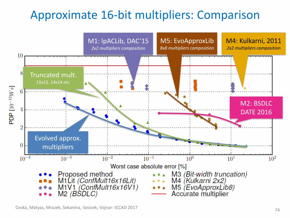
Approximate 16-bit multipliers: Comparison
74 Ceska, Matyas, Mrazek, Sekanina, Vasicek, Vojnar: ICCAD 2017
M2: BSDLC DATE 2016
M5: EvoApproxLib 8x8 multipliers composition
M4: Kulkarni, 2011 2x2 multipliers composition
M1: lpACLib, DAC’15 2x2 multipliers composition
Evolved approx. multipliers
Truncated mult. 15x15, 14x14 etc.
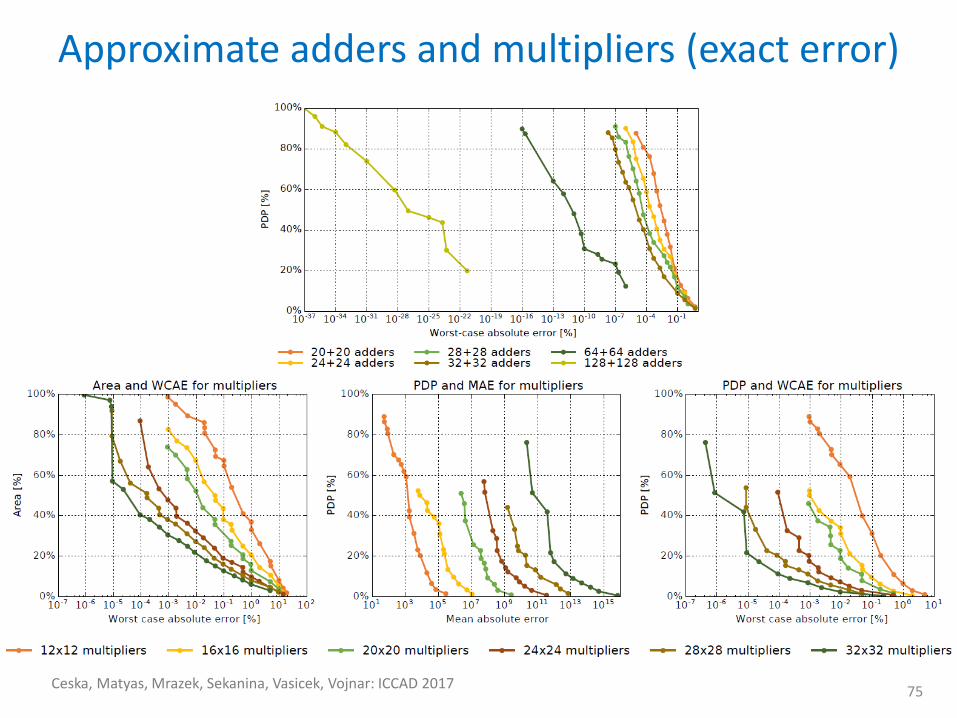
Approximate adders and multipliers (exact error)
75 Ceska, Matyas, Mrazek, Sekanina, Vasicek, Vojnar: ICCAD 2017
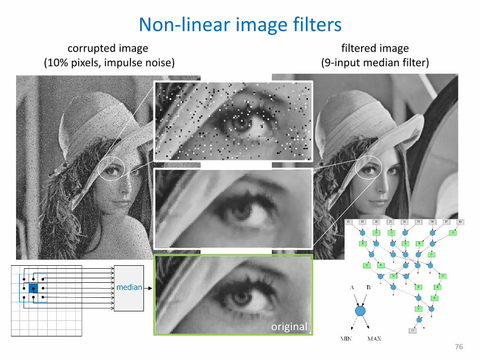
Non-linear image filters
76
filtered image (9-input median filter)
corrupted image (10% pixels, impulse noise)
original
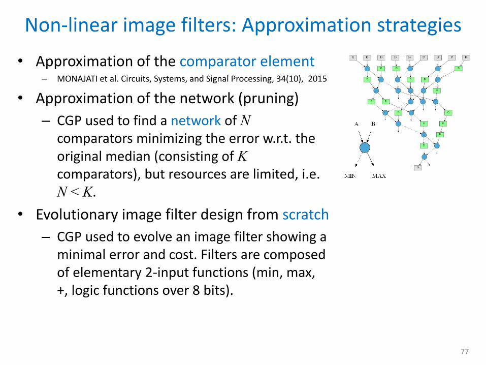
• Approximation of the comparator element – MONAJATI et al. Circuits, Systems, and Signal Processing, 34(10), 2015
• Approximation of the network (pruning)
– CGP used to find a network of N comparators minimizing the error w.r.t. the original median (consisting of K comparators), but resources are limited, i.e. N < K.
• Evolutionary image filter design from scratch
– CGP used to evolve an image filter showing a minimal error and cost. Filters are composed of elementary 2-input functions (min, max, +, logic functions over 8 bits).
Non-linear image filters: Approximation strategies
77
Approximate median using CGP
78
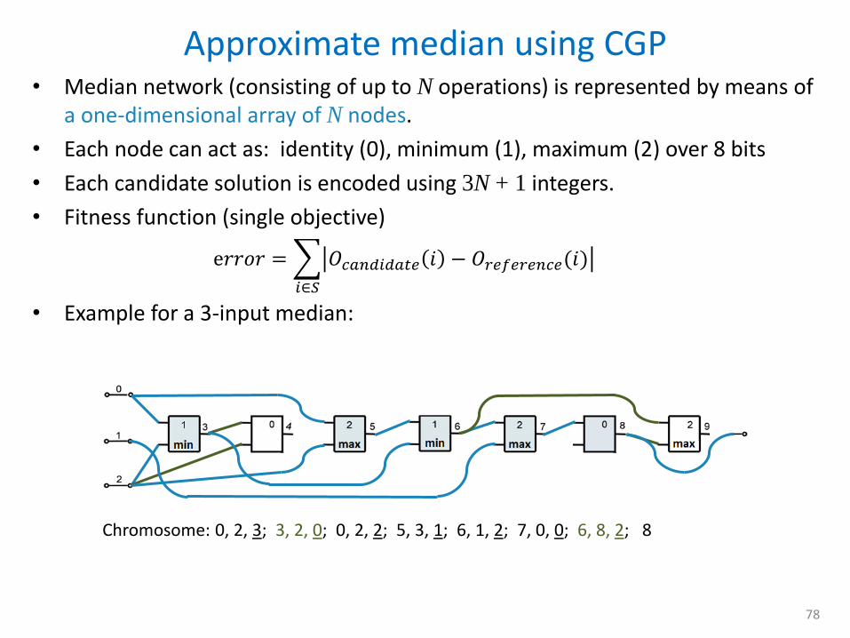
• Median network (consisting of up to N operations) is represented by means of a one-dimensional array of N nodes.
• Each node can act as: identity (0), minimum (1), maximum (2) over 8 bits
• Each candidate solution is encoded using 3N + 1 integers.
• Fitness function (single objective)
e𝑟𝑟𝑜𝑟 = 𝑂𝑐𝑎𝑛𝑑𝑖𝑑𝑎𝑡𝑒 𝑖 − 𝑂𝑟𝑒𝑓𝑒𝑟𝑒𝑛𝑐𝑒(𝑖)
𝑖∈𝑆
• Example for a 3-input median:
Chromosome: 0, 2, 3; 3, 2, 0; 0, 2, 2; 5, 3, 1; 6, 1, 2; 7, 0, 0; 6, 8, 2; 8
Approximate median using CGP
79
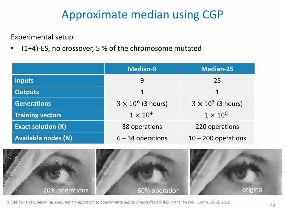
Experimental setup
• (1+4)-ES, no crossover, 5 % of the chromosome mutated
Median-9 Median-25
Inputs 9 25
Outputs 1 1
Generations 3 × 10⁶ (3 hours) 3 × 10⁵ (3 hours)
Training vectors 1 × 10⁴ 1 × 10⁵
Exact solution (K) 38 operations 220 operations
Available nodes (N) 6 – 34 operations 10 – 200 operations
60% operation 20% operations original
Z. Vašíček and L. Sekanina. Evolutionary approach to approximate digital circuits design. IEEE trans. on Evol. Comp. 19(3), 2015
Approximate median: Distance error analysis
80
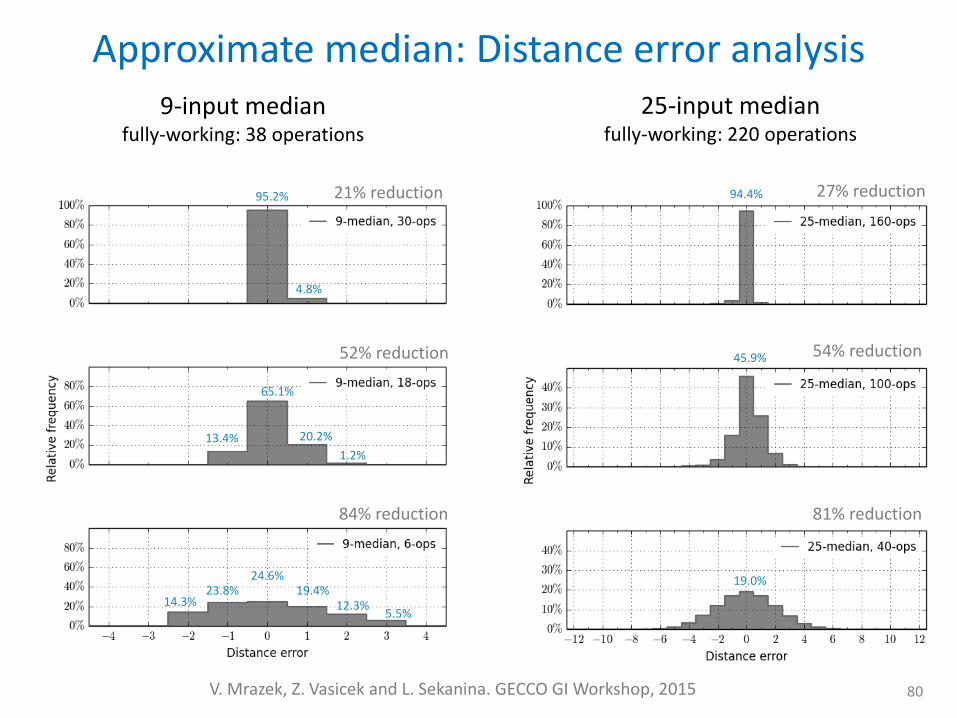
9-input median fully-working: 38 operations
25-input median fully-working: 220 operations
21% reduction
52% reduction
84% reduction
4.8%
95.2%
65.1%
24.6%
20.2% 13.4%
1.2%
23.8% 19.4% 12.3%
5.5% 14.3%
27% reduction
54% reduction
81% reduction
94.4%
45.9%
19.0%
V. Mrazek, Z. Vasicek and L. Sekanina. GECCO GI Workshop, 2015
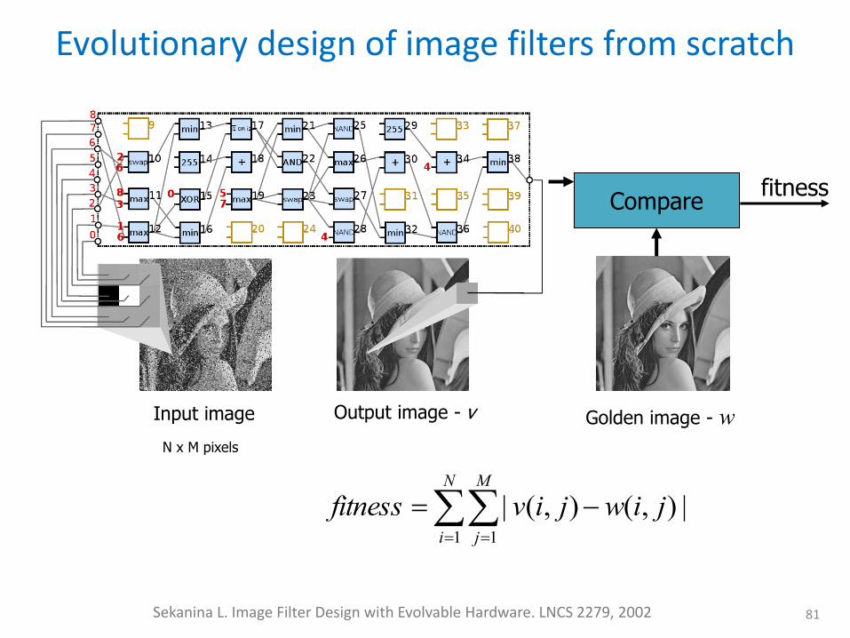
Evolutionary design of image filters from scratch
81
Golden image - w Input image
Compare fitness
N
i
M
j
jiwjivfitness1 1
|),(),(|
N x M pixels
Output image - v
Sekanina L. Image Filter Design with Evolvable Hardware. LNCS 2279, 2002
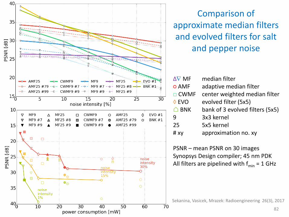
Comparison of approximate median filters and evolved filters for salt
and pepper noise
82
∆ MF median filter ○ AMF adaptive median filter □ CWMF center weighted median filter ◊ EVO evolved filter (5x5) ⌂ BNK bank of 3 evolved filters (5x5) 9 3x3 kernel 25 5x5 kernel # xy approximation no. xy PSNR – mean PSNR on 30 images Synopsys Design compiler; 45 nm PDK All filters are pipelined with fmin = 1 GHz
Sekanina, Vasicek, Mrazek: Radioengineering 26(3), 2017
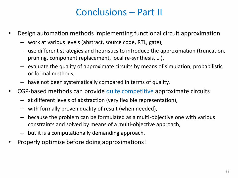
• Design automation methods implementing functional circuit approximation
– work at various levels (abstract, source code, RTL, gate),
– use different strategies and heuristics to introduce the approximation (truncation, pruning, component replacement, local re-synthesis, …),
– evaluate the quality of approximate circuits by means of simulation, probabilistic or formal methods,
– have not been systematically compared in terms of quality.
• CGP-based methods can provide quite competitive approximate circuits
– at different levels of abstraction (very flexible representation),
– with formally proven quality of result (when needed),
– because the problem can be formulated as a multi-objective one with various constraints and solved by means of a multi-objective approach,
– but it is a computationally demanding approach.
• Properly optimize before doing approximations!
Conclusions – Part II
83
• See references on particular slides
• Selected tutorial and survey papers on Approximate Computing
– J. Han and M. Orshansky, “Approximate computing: An emerging paradigm for energy-efficient design,” in Proc. of the 18th IEEE European Test Symposium. IEEE, 2013, pp. 1–6
– H. Esmaeilzadeh, A. Sampson, L. Ceze, D. Burger, “Neural acceleration for general-purpose approximate programs,” Commun. ACM, 58(1): 105-115, 2015
– S. Mittal, “A survey of techniques for approximate computing,” ACM Computing Surveys, 48(4), 1–34, 2016.
– Q. Xu, T. Mytkowicz, N. S. Kim. “Approximate Computing: A Survey,” IEEE Design and Test, 33(1), 8-22, 2016.
– L. Sekanina, “Introduction to Approximate Computing”. IEEE International Symposium on Design and Diagnostics of Electronic Circuits, DDECS 2016
– Z. Vasicek, “Relaxed equivalence checking: a new challenge in logic synthesis”. IEEE International Symposium on Design and Diagnostics of Electronic Circuits, DDECS 2017
References
84
• EHW group at Brno University of Technology
– Zdeněk Vašíček, Michal Bidlo, Roland Dobai
– Michaela Šikulová, Radek Hrbáček, Vojtěch Mrázek, David Grochol, Miloš Minařík, Jakub Husa, Marek Kidoň, Michal Wiglasz and other students
• Research funding
– IT4Innovations Centre of Excellence – National supercomputing center
– IT4Innovations excellence in science - LQ1602
– Advanced Methods for Evolutionary Design of Complex Digital Circuits, 2014 – 2016 (Czech Science Foundation)
– Relaxed equivalence checking for approximate computing, 2016 – 2018 (Czech Science Foundation)
– Brno University of Technology
Acknowledgement
85


![ASNet: Introducing Approximate Hardware to High-Level ... · [13] presents ABACUS, an automatic synthesis method for generating approx. circuits. Given a behavioral or a RTL description,](https://img.pdfslide.net/doc/110x75/5fd3cc0b50e809683d4a4051/asnet-introducing-approximate-hardware-to-high-level-13-presents-abacus.jpg)


![Local random quantum circuits are approximate polynomial ... · tary 3-designs [15], which improved on a series of papers establishing that random circuits are approximate unitary](https://img.pdfslide.net/doc/110x75/5f1f9079404b39713d0f4ee6/local-random-quantum-circuits-are-approximate-polynomial-tary-3-designs-15.jpg)