Embed Size (px)
Citation preview
8/8/2019 Approximate Option Valuation
http://slidepdf.com/reader/full/approximate-option-valuation 1/23
Journal of Financial Economics 10 (1982) 347-369. North-Holland Publishing Company
APPROXIMATE OPTION VALUATION FOR ARBITRARYSTOCHASTIC PROCESSES·
Robert JARROW and Andrew RUDD
Cornell University, Ithaca, NY 14853, USA
Received August 1981, final version received May 1982
We show how a given probability distribution can be approximated by an arbitrary distributionin terms of a series expansion involving second and higher moments. This theoreticaldevelopment is specialized to the problem of option valuation where the underlying securitydistribution, if not lognormal, can be approximated by a lognormally distributed randomvariable. The resulting option price is expressed as the sum of a Black-Scholes price plusadjustment terms which depend on the second and higher moments of the underlying securitystochastic process. This approach permits the impact on the option price of skewness andkurtosis of the underlying stock's distribution to be evaluated.
1. Introduction
The Black-Scholes (1973) formula is rightly regarded by both practitionersand academics as the premier model of option valuation. In spite of itspreeminence it has some well-known deficiencies. Empirically, model pricesappear to differ from market prices in certain systematic ways [see, e.g.,
Black (1975)]. These biases are usually ascribed to the strong assumptionthat the underlying security follows a stationary geometric Brownian motion.The implication is that at the end of any finite interval the stock price is
lognormally distributed and that over succeeding intervals the variance is
constant.The majority of the empirical evidence [e.g., Rosenberg (1972), Oldfield,
Rogalski and Jarrow (1977)] suggests that this assumption does not hold.Consequently, many theoretical option valuation models have been derivedutilizing different and (arguably) more realistic assumptions for theunderlying security stochastic process [e.g., Cox (1975), Cox and Ross (1976),
Merton (1976), Geske (1979), Rubinstein (1980)]. An alternative approach is
to estimate the underlying security distribution and then to use numerical
*This paper was presented at the Western Finance Association meetings in Jackson Hole,Wyoming. Helpful comments from George Constantinides are gratefully acknowledged. We alsothank Jim Macbeth for making his computer code (for constant elasticity of variance diffusionprocesses) available, and to Ed Bartholomew for computational assistance.
0304-405x/82/0000-0000/$02.75 © North-HollandJFE--E
9
8/8/2019 Approximate Option Valuation
http://slidepdf.com/reader/full/approximate-option-valuation 2/23
10
348 R. Jarrow and A. Rudd, Approximate option valuation
integration techniques to obtain the option price [e.g., the method ofGastineau and Madansky reported in Gastineau (1975)]. Many of these'second generation' models (either by comparative statics or empirical testing)
have been shown to (partially) explain the biases in the original Black
Scholes model.These approaches have some obvious shortcomings. For instance, the
evaluation of an option price for an arbitrary underlying distribution may be
possible only by numerical integration techniques because of the analytical
intractability of the distribution function. Empirically, it may be
straightforward to estimate the moments and other properties of the
underlying distribution, but using that information to compute option pricesmay be considerably more complex. Moreover, in both approaches it is farfrom clear how the specification of the underlying stock's distribution
manifests itself in the resulting option price, short of actually computing theoption value for all distributions of interest.
This consideration is· important because it arises for a large class of
valuation problems where the underlying distribution is itself a convolutionof other distributions. For example, the valuation of an option on a portfolioor index where the component securities are distributed 10gnormal1y.
Another example is the valuation of an option on a stock whose distributionis convoluted from the distributions of the real assets held by the corporation[Rubinstein (1980)]. In these problems, partial information concerning theunderlying distribution may be known (for instance, its moments may be
tabulated) but the distribution function itself may be so complex as to
prevent direct integration. The central question addressed here is how may
this partial information be used in obtaining option prices.In this paper we attempt to explicitly examine the impact of the underlying
distribution, summarized by its moments, on the option price. The approach
is to approximate the underlying distribution with an alternate (moretractable) distribution. In section 2 we derive the series expansion of a given
distribution in terms of an unspecified approximating distribution. Thisapproach, similar to the familiar Taylor series expansion for an analyticfunction, is called a generalized Edgeworth series expansion. It has the
desirable property that the coefficients in the expansion are simple functionsof the moments of the given and approximating distributions.
In section 3 we apply the Edgeworth series expansion to the problem of
option valuation. It is straightforward to obtain the expected value of an
option where early exercise is not optimal. In situations where risklessarbitrage is possible, Cox-Ross (1976) reasoning permits the (approximate)value of the option to be inferred from its expected value at maturity. Theapproximation in this approach results from the size of the error term in the
expansion.The final theoretical step is taken in section 4. Here we specify the
8/8/2019 Approximate Option Valuation
http://slidepdf.com/reader/full/approximate-option-valuation 3/23
R. Jarrow and A. Rudd, Approximate option valuation 349
approximating distribution to be the lognormal. Applying the results ofsection 3, the (approximate) option price is seen to be the Black-Scholesprice plus three adjustments which depend, respectively, on the differences
between the variance, skewness, and kurtosis of the underlying and the
lognormal distribution.The presence of the error term in the Edgeworth expansion indicates that
our results are only approximate. Intuition suggests that for practicalpurposes the first four moments of the underlying distribution should capturethe majority of its influence as it atTects option pricing. In section 5 we
provide some results from simulations to provide guidance when using thistechnique. For Merton's (1976) jump-diffusion option model and for Cox's
(1975) constant elasticity of diffusion model, we calculate the magnitude ofthe error term assuming, of course, that each is the true representation of
reality. The final section, section 6, concludes the paper.
2. Approximating distribution
This section modestly generalizes a technique developed by Schieher (1977)
for approximating a given probability distribution, F(s), called the truedistribution, with an alternative distribution, A(s), called the approximatingdistribution. Our generalization allows for the possibility of non-existing
moments. In the statistics literature, this technique is called a generalizedEdgeworth series expansion. The original Edgeworth series expansion [see
Cramer (1946) and Kendall and Stuart (1977)] concentrated on using thestandard normal as the approximating distribution. The following approachconsiders any arbitrary distribution A(s). For simplicity of presentation, thederivation will be performed for the restricted class of distributions where
dA(s)jds = a(s) and dF(s)jds = f(s) exist, i.e., distributions with continuousdensity functions. The derivation is generalizable; however, the presentationinvolves measure theory and is outside the scope of this paper.
The following notation will be employed:
00
rxJ{F)= S s ~ ( s ) d s , -00
00
I-LjF)= S ( s - r x l ( F » ~ ( s ) d s , (1)- 0 0
00
¢(F, t) = J eIt1(s) ds,-00
where ;2 = -1 , rxJ.F) is the jth moment of distribution F, I-LJ.F) is the jth
11
8/8/2019 Approximate Option Valuation
http://slidepdf.com/reader/full/approximate-option-valuation 4/23
12
350 R. Jarrow and A. Rudd, Approximate option valuation
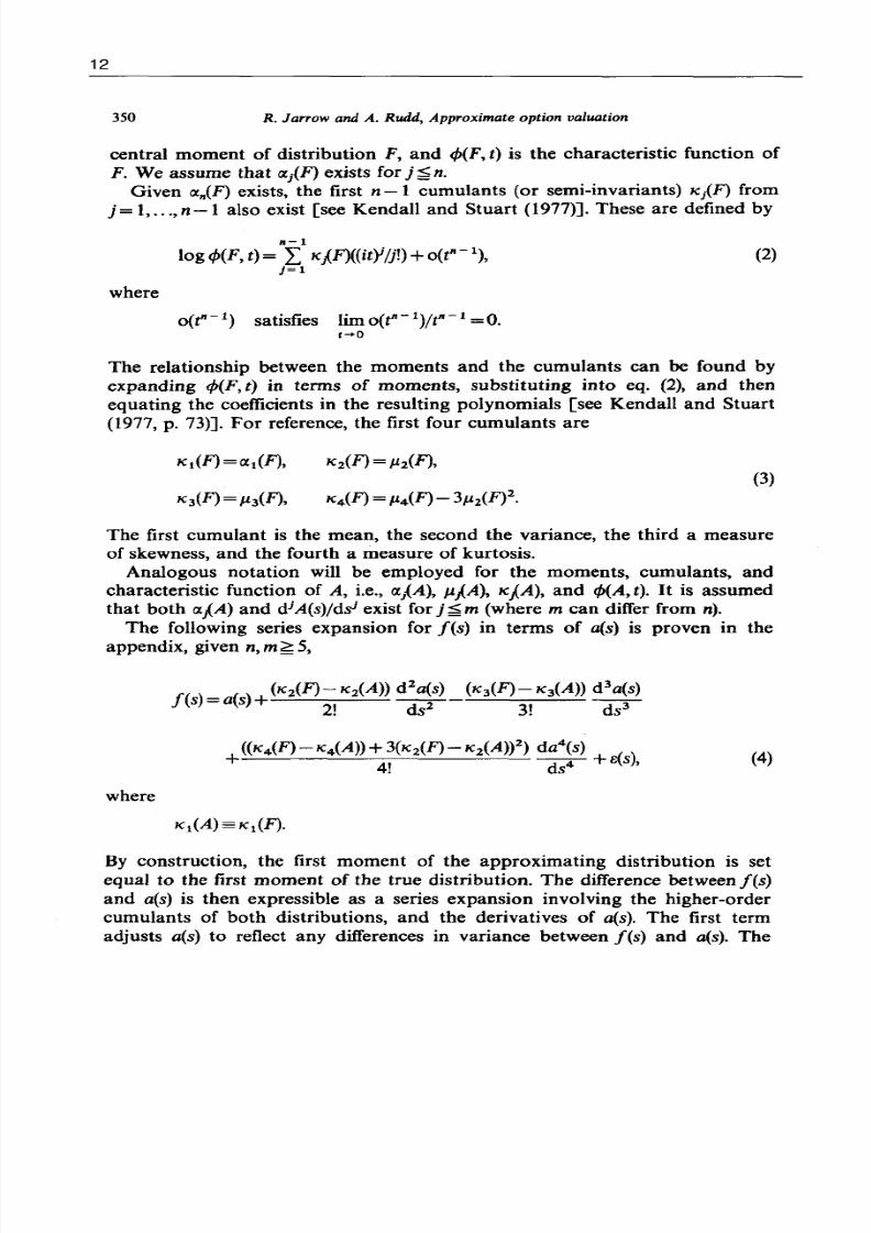
central moment of distribution F, and </J(F, t) is the characteristic function of
F. We assume that aiF) exists for j ~ n . Given aiF) exists, the first n - l cumulants (or semi-invariants) KiF) from
j= I , ... n - l also exist [see Kendall and Stuart (1977)J. These are defined by
11-1
log </J(F, t) = L KF)«itY j!) +0(1" - 1), (2)J= 1
where
0(1" -1 ) satisfies lim 0(1" -1 )/1" -1 = o.1-+0
The relationship between the moments and the cumulants can be found by
expanding </J(F, t) in terms of moments, substituting into eq. (2), and thenequating the coefficients in the resulting polynomials [see Kendall and Stuart
(1977, p. 73)J. For reference, the first four cumulants are
KiF) = JJ2(F),
(3)
K4(F) = JJ4(F) - 3JJiF)2.
The first cumulant is the mean, the second the variance, the third a measureof skewness, and the fourth a measure of kurtosis.
Analogous notation will be employed for the moments, cumulants, andcharacteristic function of A, i.e., aJ.A), JJIA), KIA), and </J(A, t). I t is assumed
that both alA) and dJA(s)/ds' exist for j ~ m (where m can differ from n).
The following series expansion for I(s) in terms of a(s) is proven in the
appendix, given n, m 5,
(4)
where
By construction, the first moment of the approximating distribution is set
equal to the first moment of the true distribution. The difference between I(s)
and a(s) is then expressible as a series expansion involving the higher-order
cumulants of both distributions, and the derivatives of a(s). The first term
adjusts a(s) to reflect any differences in variance between /(s) and a(s). The
8/8/2019 Approximate Option Valuation
http://slidepdf.com/reader/full/approximate-option-valuation 5/23
R. Jarrow and A. Rudd, Approximate option valuation 351
weighting factor is the second derivative of a(s). The second term adjusts a(s)
to account for the difference in skewness between f(s) and a(s). The weightingfactor is the third derivative. Similarly the fourth term compensates for thedifference in kurtosis and variance between the two distributions with aweighting factor of the fourth derivative. 1 Depending on the existence of thehigher moments, this expansion could be continued.
The residual error, 6(S), contains any remaining difference between the left
and right-hand sides of (4) after the series expansion. Given arbitrary trueand approximating distributions (where some moments may not exist), nogeneral analytic bounds for this error e(s,N) as a function of N (the number
of terms included) are available. For the case where all moments exist, it canbe shown (see appendix) that e(s, N)-+O uniformly in s as N -+ 00. In either
case, for finite N, the relative size of this error needs to be examined usingnumerical analysis. We will return to this issue in section 5.
3. Approximate option valuation formula
This section employs the generalized Edgeworth series expansion (4)
discussed in section 2 to obtain an approximate option valuation formula.The logic of the approach is simple. Usingf(s) as the true distribution of thestock price at maturity, the expected value at maturity of a payout protectedoption on that stock can be obtained.2 The generalized Edgeworth series
expansion then gives us an approximate expected valve for the option at
maturity in terms of the approximating distribution a(s). To obtain the value
of the option prior to maturity, we need to restrict the model such that arisk-neutrality valuation argument is valid.
Under continuous time models with no restrictions on preferences except
non-satiation, given frictionless markets and a constant term structure,necessary and sufficient conditions for this argument being valid are that thechange in both the stock's value and option's value over At are perfectlycorrelated as At-+O [see Garman (1976)]. This condition is satisfied by
Markov diffusion processes where the variance component depends on atmost the stock price and time. This includes the constant elasticity diffusion
processes as a special case [see Cox (1975)]. Simple jump processes may also
satisfy this condition [see Cox and Ross (1976)]. In addition, the argumenthas also been employed in Merton (1976) given a combined jump-diffusion
IFor any distribution, 1'4(F)= K4(F)+ K2(F)2. Consequently, the third adjustment term reflectsthe differing 'unadjusted' kurtosis between the two distributions.
2See Cox and Rubinstein (1978) for the definition of a payout protected option. For organizedexchanges, this would correspond to an American call option whose underlying stock has nodividend payments over the life of the option. The above approach could easily be generalizedto include constant dividend yields for European options or American options where theconditions are such that it is never optimal to exercise early.
13
8/8/2019 Approximate Option Valuation
http://slidepdf.com/reader/full/approximate-option-valuation 6/23
14
352 R. J arrow and A. Rudd, Approximate option valuation
process, however, also necessary is the additional restriction that the jump
risk is diversifiable. 3
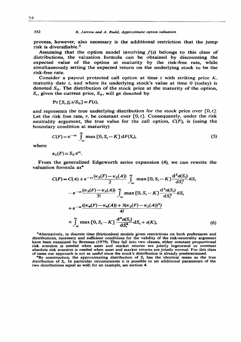
Assuming that the option model involving /(s) belongs to this class ofdistributions, the valuation formula can be obtained by discounting theexpected value of the option at maturity by the risk-free rate, whilesimultaneously setting the expected return on the underlying stock to be the
risk-free rate.Consider a payout protected call option at time t with striking price K,
maturity date t, and where its underlying stock's value at time °today) is
denoted So. The distribution of the stock price at the maturity of the option,
S/> given the current price, So, will ge denoted by
Pr [ S t ~ s / S o ] =F(s),
and represents the true underlying distribution for the stock price over [0, t].
Let the risk free rate, r, be constant over [0, t]. Consequently, under the riskneutrality argument, the true value for the call option, C(F), is (using the
boundary condition at maturity)
00C(F)=e-rr Jmax[O,St-K]dF(Sr)' (5)
-00where
From the generalized Edgeworth series expansion (4), we can rewrite thevaluation formula as4
C(F)=C(A)+e- rr (lCiF); lC2(A» ]00 max [O,Sr-K] d : i ~ t ) dSr
_ _ r(lC3(F)- lC3(A» co
J[0 S -K ] d
3a(Sr) dS
e 3! _ co max , r d S ~ t
-rr «lCiF)-lCiA»+ 3(lC2(F)- lC2(A»2)+e 4!
00 d4a(S)xJ
oo
max [O,Sr-K] d S ~ t dSr+e(K), (6)
3A1ternatively, in discrete time (frictionless) models given restrictions on both preferences anddistributions, necessary and sufficient conditions for the validity of the risk-neutrality argumenthave been examined by Brennan (1979). They fall into two classes, either constant proportionalrisk aversion is needed when asset and market returns are jointly lognormal or constantabsolute risk aversion is needed when asset and market returns are jointly normal. For this classof cases our approach is not as useful since the stock's distribution is already predetermined.
4By construction, the approximating distribution of S, has the identical mean as the truedistribution of S,. In particular circumstances it is possible to set additional parameters of thetwo distributions equal as well; for an example, see section 4.
8/8/2019 Approximate Option Valuation
http://slidepdf.com/reader/full/approximate-option-valuation 7/23
R. Jarrow and A. Rudd. Approximate option valuation 353
where00
1X 1(A)=e+rtSo and C(A)=e- r t J max [O,St-KJa(St)dSt.
- 0 0
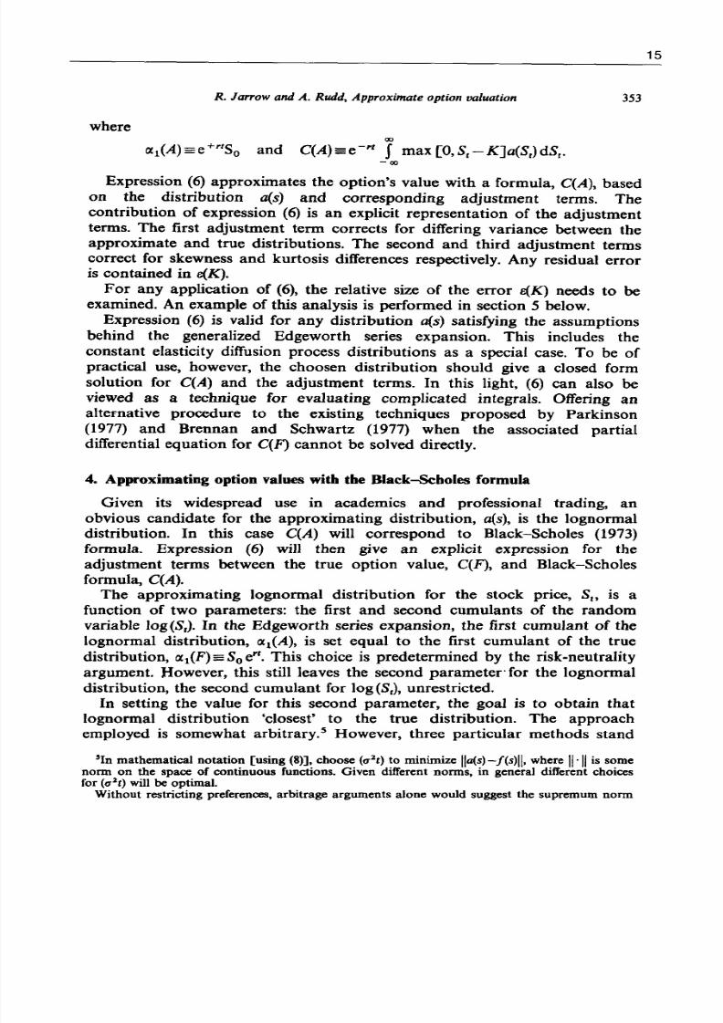
Expression (6) approximates the option's value with a formula, C(A), based
on the distribution a(s) and corresponding adjustment terms. Thecontribution of expression (6) is an explicit representation of the adjustment
terms. The first adjustment term corrects for differing variance between theapproximate and true distributions. The second and third adjustment termscorrect for skewness and kurtosis differences respectively. Any residual error
is contained ine(K).
For any application of (6), the relative size of the error e(K) needs to be
examined. An example of this analysis is performed in section 5 below.
Expression (6) is valid for any distribution a(s) satisfying the assumptions
behind the generalized Edgeworth series expansion. This includes the
constant elasticity diffusion process distributions as a special case. To be of
practical use, however, the choosen distribution should give a closed formsolution for C(A) and the adjustment terms. In this light, (6) can also be
viewed as a technique for evaluating complicated integrals. Offering an
alternative procedure to the existing techniques proposed by Parkinson(1977) and Brennan and Schwartz (1977) when the associated partialdifferential equation for C(F) cannot be solved directly.
4. Approximating option values with the Black-8cboles formula
Given its widespread use in academics and professional trading, anobvious candidate for the approximating distribution, a(s), is the lognormaldistribution. In this case C(A) will correspond to Black-Scholes (1973)
formula. Expression (6) will then give an explicit expression for the
adjustment terms between the true option value, C(F), and Black-Scholesformula, C(A).
The approximating lognormal distribution for the stock price, S" is afunction of two parameters: the first and second cumulants of the randomvariable 10g(St). In the Edgeworth series expansion, the first cumulant of thelognormal distribution, 1X 1(A), is set equal to the first cumulant of the true
distribution, 1X 1(F)=Soe,t. This choice is predetermined by the risk-neutrality
argument. However, this still leaves the second parameter' for the lognormal
distribution, the second cumulant for 10g(St), unrestricted.
In setting the value for this second parameter, the goal is to obtain thatlognormal distribution 'closest' to the true distribution. The approachemployed is somewhat arbitrary. S However, three particular methods stand
'In mathematical notation [using (8)]. choose (qlt) to minimize lIa(s) -/(s)lI. where 11'11 is somenorm on the space of continuous functions. Given different norms. in general different choicesfor (q 2t) will be optimal.
Without restricting preferences. arbitrage arguments alone would suggest the supremum norm
15
8/8/2019 Approximate Option Valuation
http://slidepdf.com/reader/full/approximate-option-valuation 8/23
16
354 R. Ja"ow and A. Rudd, Approximate option valuation
out. The first is to equate the second cumulant of the approximating
lognormal to the true distribution's second cumulant, i.e., " iA ) == "2(F). Thiscompletely specifies the second parameter for the lognormal distribution. Thesecond approach is to directly equate the second cumulants of log (S,) for theapproximating lognormal and the true distribution. Both of these approachesconsider cumulants over the entire interval [0, tJ. A third approach is toequate the instantaneous variances over [0, LI t] as Llt--+O. In this case both
the instantaneous return variance and the instantaneous logarithmic variance
are equal.The three approach will give different approximating distributions, a(s).
This paper demonstrates the second approach, equating the cumulants of(log S,). This is done, in part, so that the resulting approximating formula is
useful in explaining the empirical evidence contained in Black and Scholes
(1975), Macbeth and Merville (1980), and most other empirical tests. These
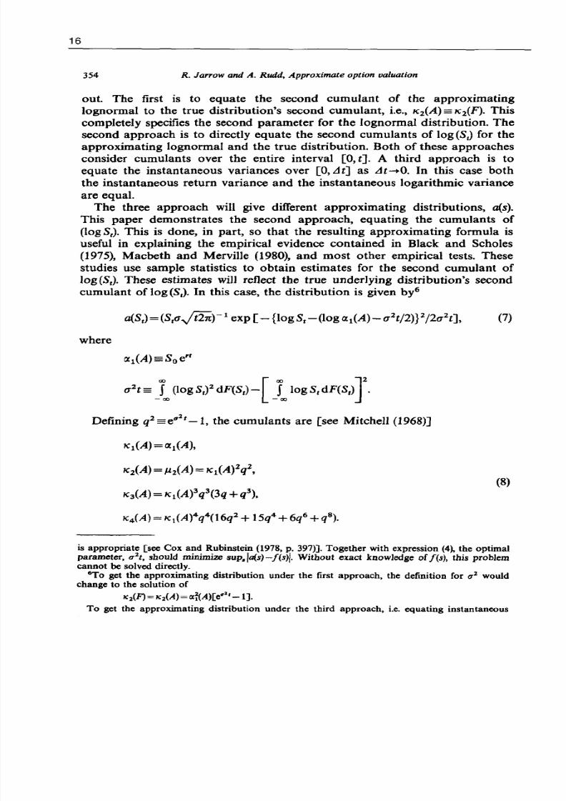
studies use sample statistics to obtain estimates for the second cumulant oflog (S,). These estimates will reflect the true underlying distribution's secondcumulant of log (S,). In this case, the distribution is given by6
where
Defining q2==e,,2 t_ 1, the cumulants are [see Mitchell (1968)J
"1(A)=a:1(A),
" iA ) = Jl2(A) = "1(A)2q2,
"3(A)=" 1(A)3 q3(3q+q3),
(8)
is appropriate [see Cox and Rubinstein (1978, p. 397)]. Together with expression ( 4 ~ the optimalparameter, q
2t, should minimize suP./a(s)-!(s)/. Without exact knowledge of !(s), this problem
cannot be solved directly.6To get the approximating distribution under the first approach, the definition for q2 would
change to the solution of
"2(F) = " i A ) = I X ~ ( A ) [ e " ' / - 1 ] . To get the approximating distribution under the third approach, i.e. equating instantaneous
8/8/2019 Approximate Option Valuation
http://slidepdf.com/reader/full/approximate-option-valuation 9/23
R. Jarrow and A. Rudd, Approximate option valuation 355
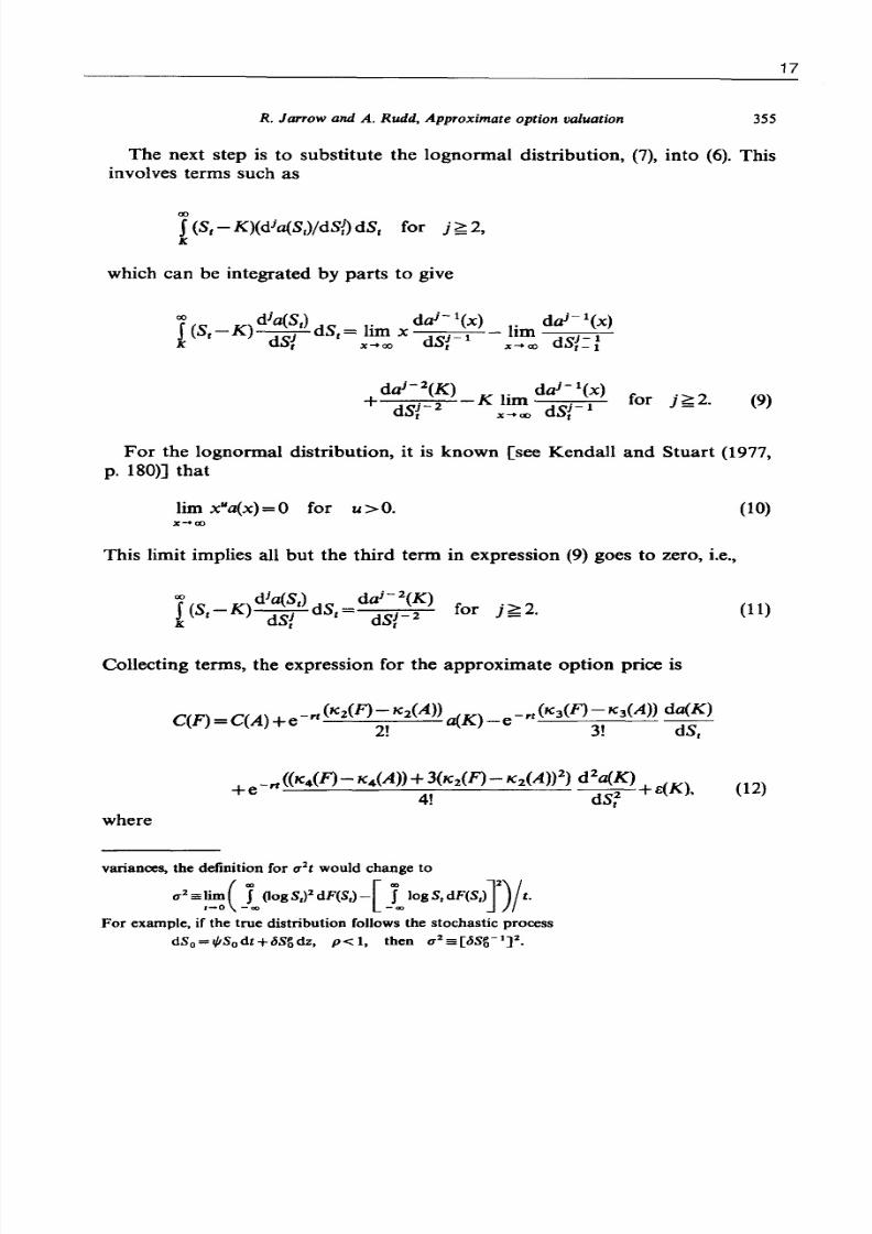
The next step is to substitute the lognormal distribution, (7), into (6). This
involves terms such as
co
f (S,-K)(dia(S,)/dSf)dS, for j"?,2,K
which can be integrated by parts to give
COf (S _K)dia(S,) dS = l' dai-
1(x)
, dSJ , Imx dSJ 1K t . x ~ C ( ) r
daJ-2(K) . dai- 1(x)
+ dsi 2 K hm dsi 1 for j"?,2. (9)t X"" 00 t
For the lognormal distribution, it is known [see Kendall and Stuart (1977,
p. 180)] that
lim x"a(x)=O for u>O.X '" co
This limit implies all but the third term in expression (9) goes to zero, i.e.,
Collecting terms, the expression for the approximate option price is
where
variances, the definition for (12t would change to
( 1 2 = ~ ~ ( I (I0gS,)2 dF(SJ- [ J.., log S, dF(S,)J)!t.For example, if the true distribution follows the stochastic process
dSo=y,Sodt+c5sgdz, p< I, then (12= [c5Sg- I]2.
(to)
(11)
(12)
17
8/8/2019 Approximate Option Valuation
http://slidepdf.com/reader/full/approximate-option-valuation 10/23
18
356 R. Jarrow and A. Rudd. Approximate option valuation
C(A) = SoN(d) - K e -rrN(d - (10),
d log (So/K e-rl) +q2 t/2
(10
N( . )= cumulative standard normal.
Expression (12) gives three adjustment terms to the Black-Scholes
valuation formula which will bring its value closer to the true option value
[up to error e(K)].
The first adjustment term corrects for differing variance. I f the truedistribution has a larger variance than the approximating lognormal, then
this term is positive. The size of the adjustment term depends on the
magnitude of the approximating density function at the exercise price, a{,K).
This value depends on whether the stock price is in or out of the money, and
how deep it is in or out of the money. An option is in the money if
So>Ke-rl
, at the money if So=Ke- r' , or out of the money if So<Ke- rl•
Since the mean of the distribution is So err, one can classify in/at/out of
money as to whether
[out of the money],
[at the money], (13)
[in the money].
Using fig. 1 for reference, the at the money options will have a larger first
adjustment term [due to the factor a{,K)] than deep in or deep out of the
money options.The second term corrects for differing skewness. Its sign depends on
whether the true distribution is more skewed than the approximating
lognormal and the sign of the lognormal's first derivative evaluated at K.
Using fig. 1, this derivative changes signs. It is positive if K <mode of
lognormal, where
Mode =ocl(A)e-3"z,/2. (14)
The maximum absolute adjustment due to this term occurs at the first andsecond inflection points, i.e.,
Inflection points = (mode) e(-"Zt/2)[1 +[1 ±4/"Zr] t ] . (15)
These will correspond to deep in (1st inflection) and deep out (2nd inflection)
8/8/2019 Approximate Option Valuation
http://slidepdf.com/reader/full/approximate-option-valuation 11/23
o(K)
o'(K)
o"(K)
R. Jarrow and A. Rudd, Approximate option valuation
lSIinflection
I
deep in
the money
mean
IIIIIIII
01 the
money
2nd infleclionpain!
III
IIIIIIII
III
deep oul of
th e money
357
K
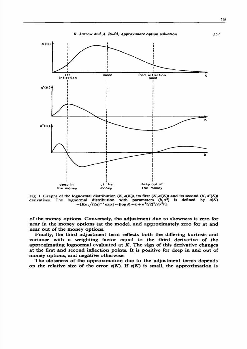
Fig. 1. Graphs of the lognormal distribution (K,a(K»' its first (K,a'(K» and its second (K,a"(K»derivatives. The lognormal distribution with parameters (b,u2
) is defined by a(K)
=(Ku.Jt2n)-lcxp [-(logK - b+u1t/2)1/2u1tJ.
of the money options. Conversely, the adjustment due to skewness is zero fornear in the money options (at the mode), and approximately zero for at andnear out of the money options.
Finally, the third adjustment term reflects both the differing kurtosis and
variance with a weighting factor equal to the third derivative of theapproximating lognormal evaluated at K. The sign of this derivative changesat the first and second inflection points. I t is positive for deep in and out ofmoney options, and negative otherwise.
The closeness of the approximation due to the adjustment terms dependson the relative size of the error e(K). I f e(K) is small, the approximation is
19
8/8/2019 Approximate Option Valuation
http://slidepdf.com/reader/full/approximate-option-valuation 12/23
20
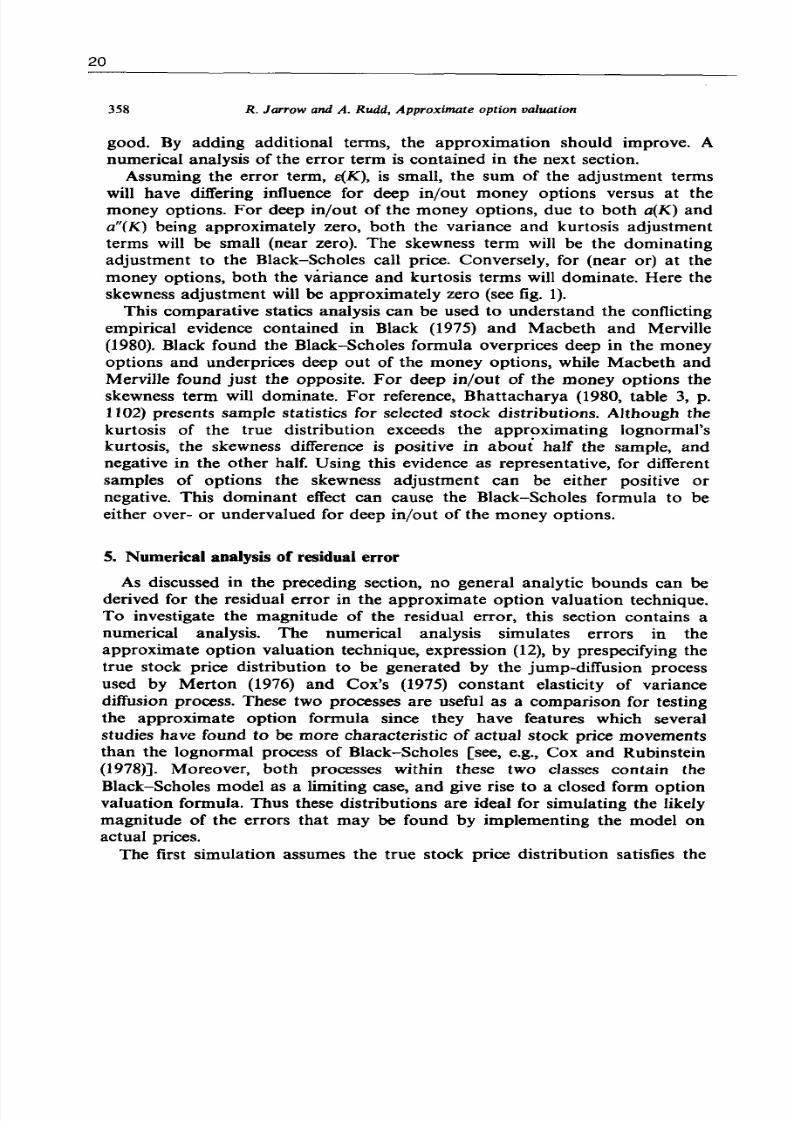
358 R. Jarrow and A. Rudd, Approximate option valuation
good. By adding additional terms, the approximation should improve. Anumerical analysis of the error term is contained in the next section.
Assuming the error term, e(K), is small, the sum of the adjustment termswill have differing influence for deep in/out money options versus at themoney options. For deep in/out of the money options, due to both a(K) anda"(K) being approximately zero, both the variance and kurtosis adjustmentterms will be small (near zero). The skewness term will be the dominating
adjustment to the Black-Scholes call price. Conversely, for (near or) at the
money options, both the variance and kurtosis terms will dominate. Here the
skewness adjustment will be approximately zero (see fig. 1).
This comparative statics analysis can be used to understand the conflictingempirical evidence contained in Black (1975) and Macbeth and Merville
(1980). Black found the Black-Scholes formula overprices deep in the moneyoptions and underprices deep out of the money options, while Macbeth and
MerviHe found just the opposite. For deep in/out of the money options theskewness term will dominate. For reference, Bhattacharya (1980, table 3, p.
1102) presents sample statistics for selected stock distributions. Although thekurtosis of the true distribution exceeds the approximating lognormal'skurtosis, the skewness difference is positive in about half the sample, and
negative in the other half. Using this evidence as representative, for differentsamples of options the skewness adjustment can be either positive or
negative. This dominant effect can cause the Black-Scholes formula to beeither over- or undervalued for deep in/out of the money options.
5. Numerieal analysis of residual error
As discussed in the preceding section, no general analytic bounds can be
derived for the residual error in the approximate option valuation technique.
To investigate the magnitude of the residual error, this section contains anumerical analysis. The numerical analysis simulates errors in theapproximate option valuation technique, expression (12), by prespecifying the
true stock price distribution to be generated by the jump-diffusion processused by Merton (1976) and Cox's (1975) constant elasticity of variance
diffusion process. These two processes are useful as a comparison for testing
the approximate option formula since they have features which severalstudies have found to be more characteristic of actual stock price movementsthan the lognormal process of Black-Scholes [see, e.g., Cox and Rubinstein
(1978)]. Moreover, both processes within these two classes contain theBlack-Scholes model as a limiting case, and give rise to a closed form option
valuation formula. Thus these distributions are ideal for simulating the likelymagnitUde of the errors that may be found by implementing the model onactual prices.
The first simulation assumes the true stock price distribution satisfies the
8/8/2019 Approximate Option Valuation
http://slidepdf.com/reader/full/approximate-option-valuation 13/23
R. Jarrow and A. Rudd. Approximate option valuation
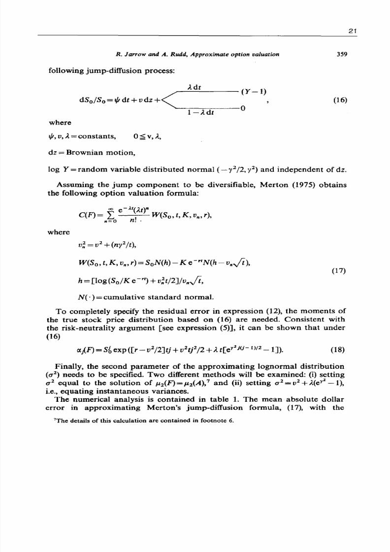
following jump-diffusion process:
,...-_A._d_t___ Y- I )
dSo/So= '" dt + vdz+(-----,,----0
l - l d t
where
1/1, v, l = constants, O ~ V , A . ,
dz =Brownian motion,
359
(16)
log Y= random variable distributed normal ( - y2/2, y2) and independent of dz.
Assuming the jump component to be diversifiable, Merton (1975) obtains
the following option valuation formula:
where
W(So, t, K, Vn, r) =SoN(h) - K e -rW(h - vn.ji).
h = [log (So/K e-rt
) + v;t/2J/v".ji,
N( . ) = cumulative standard normal.
(17)
To completely specify the residual error in expression (12), the moments of
the true stock price distribution based on (16) are needed. Consistent with
the risk-neutrality argument [see expression (5)], it can be shown that under
(16)
(18)
Finally, the second parameter of the approximating lognormal distribution
(0'2) needs to be specified. Two different methods will be examined: (i) setting
0'2 equal to the solution of 1J.z{F)=1J.2(A)/ and (ii) setting O'2=v2+l(ey2_1),
i.e., equating instantaneous variances.
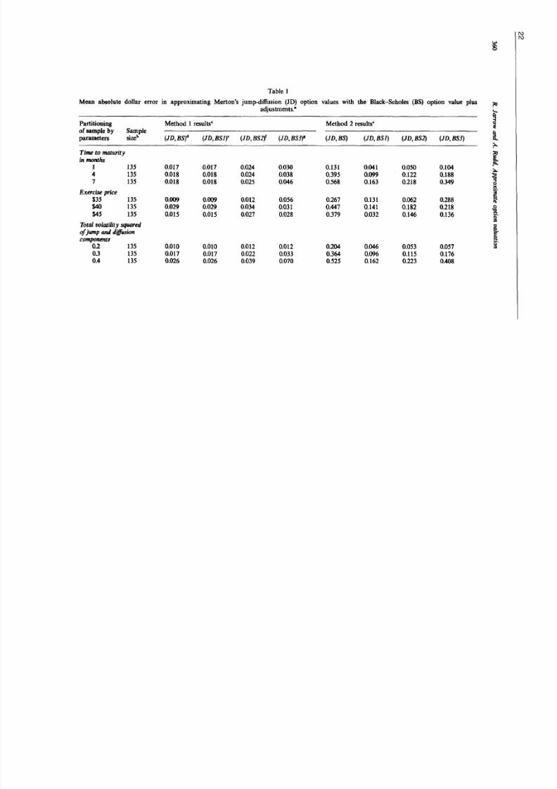
The numerical analysis is contained in table 1. The mean absolute dollar
error in approximating Merton's jump-diffusion formula, (17), with the
7The details of this calculation are contained in footnote 6.
21
8/8/2019 Approximate Option Valuation
http://slidepdf.com/reader/full/approximate-option-valuation 14/23
Table 1
Mean absolute dollar error in approximating Merton's jump-difJusion (JD) option values with the Black-Scholes (BS) option value plusadjustments.'
Partitioning Method 1 results· Method 2 results·ofsantple by Sample
parameters sizeb (JD,BS)d (JD, BSl)C (JD,BS2f (JD,BS3), (JD,BS) (JD, BSl) (JD,BS2) (JD,BS3)
Time to maturityin months
1 135 0.017 0.017 0.024 0.030 0.131 0.041 0.050 0.1044 135 O.ot8 O.ot8 0.024 0.Q38 0.395 0.099 0.122 0.1887 135 O.ot8 O.ot8 0.025 0.046 0.568 0.163 0.218 0.349
Exercise price$35 135 0.009 0.009 0.012 0.056 0.267 0.131 0.062 0.288$40 135 0.029 0.029 0.034 0.031 0.447 0.141 0.182 0.218$45 135 O.ot5 Om5 0.027 0.Q28 0.379 0.032 0.146 0.136
Total IJOlatility squaredof ump and diffusioncomponents
02 135 0.010 0.010 0.012 0.012 0.204 0.046 0.053 0.0570.3 135 0.017 0.017 0.022 0.033 0.364 0.096 0.115 0.1760.4 135 0.026 0.026 0.039 0.070 0.525 0.162 0.223 0.408
w
8J
!I:.
s..?o-):I
Ics·:s
!aCS·:s
I\ )
I\ )
8/8/2019 Approximate Option Valuation
http://slidepdf.com/reader/full/approximate-option-valuation 15/23
8/8/2019 Approximate Option Valuation
http://slidepdf.com/reader/full/approximate-option-valuation 16/23
24
362 R. Jarrow and A. Rudd, Approximate option valuation
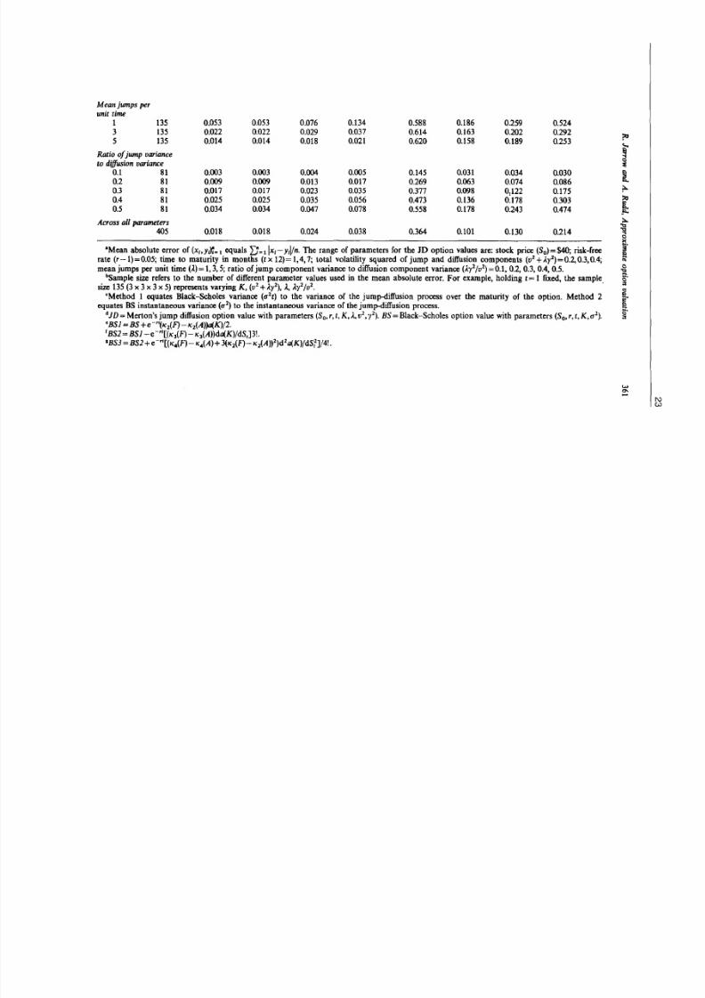
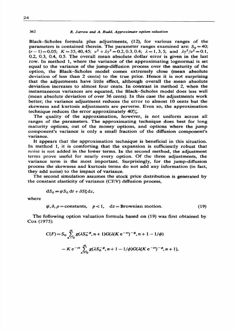
Black-Scholes formula plus adjustments, (12), for various ranges of the
parameters is contained therein. The parameter ranges examined are: So =40;
(r-l)=0.05; K=35,40,45; v2+A.l =0.2,0.3,0.4; ),=1,3,5; and A.y2/v2=O.I,
0.2, 0.3, 0.4, 0.5. The overall mean absolute dollar error is given in the last
row. In method 1, where the variance of the approximating lognormal is set
equal to the variance of the jump-diffusion process over the maturity of the
option, the Black-Scholes model comes extremely close (mean absolute
deviation of less than 2 cents) to the true price. Hence it is not surprising
that the adjustments have little effect, although overall the mean absolute
deviation increases to almost four cents. In contrast in method 2, when the
instantaneous variances are equated, the Black-Scholes model does less well(mean absolute deviation of over 36 cents). In this case the adjustments work
better; the variance adjustment reduces the error to almost 10 cents but the
skewness and kurtosis adjustments are perverse. Even so, the approximation
technique reduces the error approximately 40%.
The quality of the approximation, however, is not uniform across all
ranges of the parameters. The approximating technique does best for long
maturity options, out of the money options, and options where the jump
component's variance is only a small fraction of the diffusion component's
variance.It appears that the approximation technique is beneficial in this situation.
In method 1, it is comforting that the expansion is sufficiently robust that
noise is not added in the lower terms. In the second method, the adjustment
terms prove useful for nearly every option. Of the three adjustments, the
variance term is the most important. Surprisingly, for the jump-diffusion
process the skewness and kurtosis terms do not add any information (in fact,
they add noise) to the impact of variance.
The second simulation assumes the stock price distribution is generated by
the constant elasticity of variance (CEV) diffusion process,
where
t/I,b,p=constants, p<l, dz=Brownian motion. (19)
The following option valuation formula based on (19) was first obtained by
Cox (1975):
00
C(F) = So L g(ASo"', n+ I)G(A(K e -rt) -"', n+ 1-1/<1»n=O
00
- K e -r t L g(ASo"', n+1-1/tP)G(A(K e -'t) -<P, n+ 1),n=O
8/8/2019 Approximate Option Valuation
http://slidepdf.com/reader/full/approximate-option-valuation 17/23
where
R. Jarrow and A. Rudd, Approximate option valuation
4>=2p-2,
00
r(n)= f e -vV, , - l dv,o
00
G(w,n)= Jg(z,n)dz.w
363
(20)
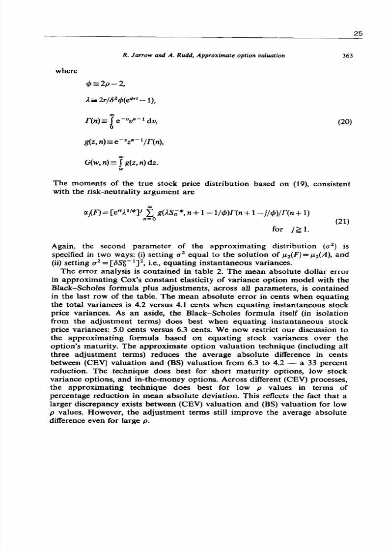
The moments of the true stock price distribution based on (19), consistentwith the risk-neutrality argument are
00
IXP')= [enA1/"]l L g(ASC;", n+ I-1jcp)F(n +1 - j/4»/F(n + 1), ,=0
(21)
for 1.
Again, the second parameter of the approximating distribution (0"2) is
specified in two ways: (i) setting 0"2 equal to the solution of Jl.iF)::: Jl.2(A), and
(ii) setting 0"2 = [bSg - 1] 2, i.e., equating instantaneous variances.
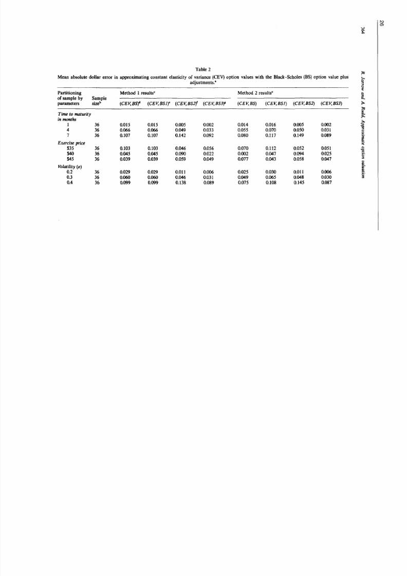
The error analysis is contained in table 2. The mean absolute dollar error
in approximating Cox's constant elasticity of variance option model with the
Black-Scholes formula plus adjustments, across all parameters, is contained
in the last row of the table. The mean absolute error in cents when equating
the total variances is 4.2 versus 4.1 cents when equating instantaneous stock
price variances. As an aside, the Black-Scholes formula itself (in isolation
from the adjustment terms) does best when equating instantaneous stock
price variances: 5.0 cents versus 6.3 cents. We now restrict our discussion to
the approximating formula based on equating stock variances over the
option's maturity. The approximate option valuation technique (including all
three adjustment terms) reduces the average absolute difference in cents
between (CEV) valuation and (BS) valuation from 6.3 to 4.2 - a 33 percent
reduction. The technique does best for short maturity options, low stock
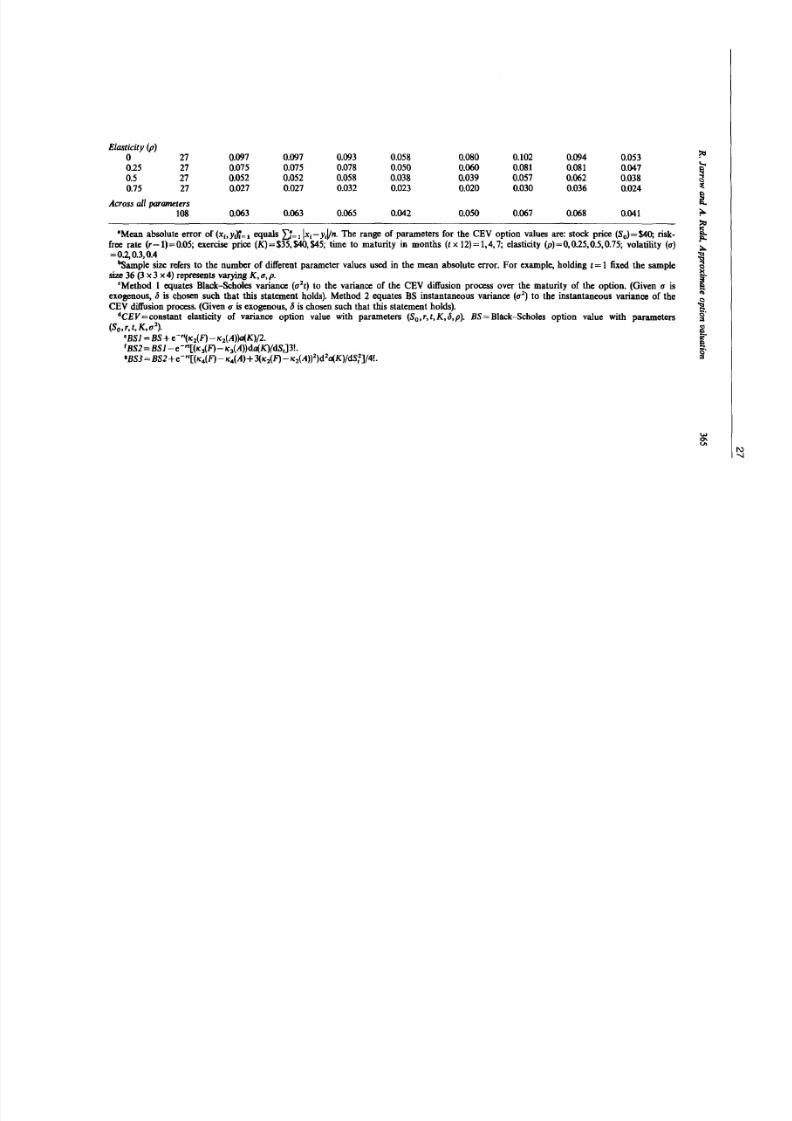
variance options, and in-the-money options. Across different (CEV) processes,the approximating technique does best for low p values in terms of
percentage reduction in mean absolute deviation. This reflects the fact that a
larger discrepancy exists between (CEV) valuation and (BS) valuation for low
p values. However, the adjustment terms still improve the average absolute
difference even for large p.
25
8/8/2019 Approximate Option Valuation
http://slidepdf.com/reader/full/approximate-option-valuation 18/23
Table 2
Mean absolute dollar error in approximating constant elasticity of variance (CEV) option values with the Black-Scholes (BS) option value plusadjustments."
Partitioning Method 1 results· Method 2 results·of
sample by Sampleparameters sizeb
(CEV,Bst (CEV,BSl)' (CEV,BS2f (CEV,BS3)" (CEY,BS) (CEY, BSJ) (CEV,BS2) (CEV,BS3)
Time to maturity
in months
1 36 0.015 0.015 0.005 0.002 0.014 0.016 0.005 0.0024 36 0.066 0.066 0.049 0.033 0.055 0.070 0.050 0.0317 36 0.107 0.107 0.142 0.092 0.080 0.117 0.149 0.089
Exercise price
$35 36 0.103 0.103 0.046 0.056 0.070 0.112 0.052 0.051$40 36 0.045 0.045 0.090 0.022 0.002 0.047 0.094 0.025$45 36 0.039 0.039 0.059 0.049 0.077 0.043 0.058 0.047
Volatility (0')
0.2 36 0.029 0.029 0.011 0.006 0.025 0.030 0.011 0.006OJ 36 0.060 0.060 0.046 0.031 0.049 0.065 0.048 0.0300.4 36 0.099 0.099 0.138 0.089 0.075 0.108 0.145 0.087
.....El...c
'"sI>...
?o-
>:l
:..
['"c
c·:s
fac·:s
I\.)
0)
8/8/2019 Approximate Option Valuation
http://slidepdf.com/reader/full/approximate-option-valuation 19/23
Elasticity (P)0 27 0.097 0.097 0.093 0.058 0.080 0.102 0.094 0.0530.25 27 0.075 0.075 0.078 0.050 0.060 0.081 0.081 0.0470.5 27 0.052 0.052 0.058 0.038 0.039 0.057 0.062 0.0380.75 27 0.027 0.027 0.032 0.023 0.020 0.030 0.036 0.024
Across all parameters
108 0.063 0.063 0.065 0.042 0.050 0.067 0.068 0.041
"Mean absolute error of (Xh y l f t ~ 1 equals 1 IXI- yMn. The range of parameters for the CEV option values are: stock price (So) = S4O; riskfree rate (r-l)=0.05; exercise price (K)=$35,$40,$45; time to maturity in months (t x 12)= 1,4, 7; elasticity (P)=0,0.25,0.5,0.75; volatility (u)
= 0.2, 0.3, 0.4"Sample size refers to the number of different parameter values used in the mean absolute error. For example, holding t= 1 fixed the sample
size 36 (3 x 3 x4) represents varying K,u,p.
"Method 1 equates Black-Scholes variance (u2 t) to the variance of the CEV diffusion process over the maturity of the option. (Given u is
exogenous, lJ is chosen such that this statement holds). Method 2 equates BS instantaneous variance (u 2) to the instantaneous variance of the
CEV diffusion process. (Given u is exogenous, lJ is chosen such that this statement holds).dCEV=constant elasticity of variance option value with parameters (So,r,t,K,lJ,p). BS=Black-Scholes option value with parameters
(So,r,t,K,,,.2).
CBS1 =BS+ e-"(K2(F)-K2(A»)a(K)f2.rBS2=BSI-e "[(K3(F)-KiA»da(K)/dS,]3!'IBS3 = BS2+e -"[(K4(F) - K4(A) + 3(K2(F) - K2(A»2Wa(K)/dSf]/4!.
!1;...i1
1-
....'"I I\ )
-...J
8/8/2019 Approximate Option Valuation
http://slidepdf.com/reader/full/approximate-option-valuation 20/23
28
366 R. Jarrow and A. Rudd, Approximate option valuation
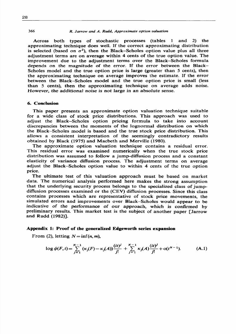
Across both types of stochastic processes (tables 1 and 2) the
approximating technique does well. I f the correct approximating distributionis selected (based on 0"2), then the Black-Scholes option value plus all three
adjustment terms are on average within 4 cents of the true option value. The
improvement due to the adjustment terms over the Black-Scholes formuladepends on the magnitude of the error. I f the error between the Black
Scholes model and the true option price is large (greater than 5 cents), thenthe approximating technique on average improves the estimate. I f the error
between the Black-Scholes model and the true option price is small (less
than 5 cents), then the approximating technique on average adds noise.
However, the additional noise is not large in an absolute sense.
6. Conclusion
This paper presents an approximate option valuation technique suitable
for a wide class of stock price distributions. This approach was used to
adjust the Black-Scholes option pricing formula to take into account
discrepancies between the moments of the lognormal distribution on whichthe Black-Scholes model is based and the true stock price distribution. This
allows a consistent interpretation of the seemingly contradictory resultsobtained by Black (1975) and Macbeth and Merville (1980).
The approximate option valuation technique contains a residual error.
This residual error was examined numerically when the true stock price
distribution was assumed to follow a jump-diffusion process and a constant
elasticity of variance diffusion process. The adjustment terms on average
adjust the Black-Scholes option value to within 4 cents of the true optionprice.
The ultimate test of this valuation approach must be based on market
data. The numerical analysis performed here makes the strong assumptionthat the underlying security process belongs to the specialized class of jump
diffusion processes examined or the (CEV) diffusion processes. Since this class
contains processes which are representative of stock price movements, the
simulated errors and improvements over Black-Scholes would appear to be
indicative of the performance of our approach, which is confirmed by
preliminary results. This market test is the subject of another paper [Jarrowand Rudd (1982)].
Appendix 1: Proof of the generalized Edgeworth series expansion
From (2), letting N =inf(n,m),
8/8/2019 Approximate Option Valuation
http://slidepdf.com/reader/full/approximate-option-valuation 21/23
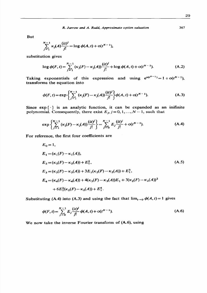
R. Jarrow and A. Rudd, Approximate option valuation 367
But
N-l (itYL KjA)-.-, =logl/J(A,t)+o(t
N-
1),
j= 1 J.
substitution gives
N-l (itYlogl/J(F,t)= L (K
1{F)-K
1{A»-.-,+logl/J(A,t)+o(t
N-
1). (A.2)
j = 1 J.
Taking exponentials of this expression and using eo(tN-I) = 1+ o(tN - 1),
transforms the equation into
{
N-l (itY}I/J(F, t)=exp (KjF)-KjA»-.,- I/J(A, t)+o(t
N-
1).
} -1 J.(A.3)
Since exp { .} is an analytic function, it can be expanded as an inifinite
polynomial. Consequently, there exist Ej , j = 0,1, ... N -1 , such that
(A.4)
For reference, the first four coefficients are
Eo=l,
El =(Kl(F)- Kl(A»,
E2 =(K2(F)- K2(A»+Ef, (A.5)
E3 =(K3(F)- K3(A» + 3 E l ( K 2 ( F ) - K i A » + E ~ , E4 =(K4(F)- K4(A» +4(KiF) -K3(A»El +3(K2(F) - K2(A»2
+ 6Ef(K2(F) - KiA» +E1·
Substituting (AA) into (A.3) and using the fact that lim, ...o I/J(A, t) = 1 gives
(A.6)
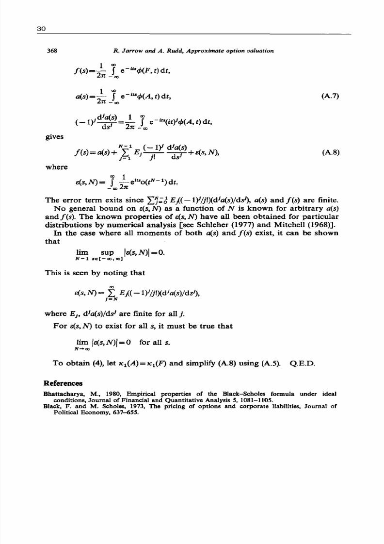
We now take the inverse Fourier transform of (A.6), using
29
8/8/2019 Approximate Option Valuation
http://slidepdf.com/reader/full/approximate-option-valuation 22/23
30
368
gives
where
R. Jarrow and A. Rudd, Approximate option valuation
1 co
f(s) =-2 f e-1t'cp(F,t)dt,7t - co
1 co
a(s)=-2 f e-ltscp(A, t)dt,7t - co
N-1 (-1)' d1
a(s)f(s)=a(s)+ L E1-.,- d- f +e(s,N),1=1 J. / ) ~
co 1e(s,N)= f - e l t ' o ( ~ - l ) d t .
- co 27 t
(A.7)
{A.8)
The error term exits since r1:J Et( -1)'/jl)(d1a(s)/dsi), a(s) and /(s) are finite.
No general bound on e(s,N) as a function of N is known for arbitrary a(s)
and /(s). The known properties of e(s, N) have all been obtained for particular
distributions by numerical analysis [see SchIeher (1977) and Mitchell (1968)].In the case where all moments of both a(s) and /(s) exist, it can be shown
that
lim sup Ie(s, N)I = o.
N-11e[-co.co)
This is seen by noting that
co
e(s,N)= L Et(-I)'/jIXdJa(s)/dsl),j=N
where E1, d1a(s)/dsf are finite for all j.
For e(s, N) to exist for all s, it must be true that
lim Ie(s, N)I =0 for all s.N-+co
To obtain (4), let "l(A) = "1(F) and simplify (A.8) using (A.5). Q.E.D.
References
Bhattacharya, M., 1980, Empirical properties of the Black-5choles formula under idealconditions, Journal of Financial and Quantitative Analysis 5, 1081-1105.
Black, F. and M. Scholes, 1973, The pricing of options and corporate liabilities, Journal ofPolitical Economy, 637-655.
8/8/2019 Approximate Option Valuation
http://slidepdf.com/reader/full/approximate-option-valuation 23/23