Approximate Query Processing: Techniques & Applications Presented by- Shraddha Rumade

Approximate Query Processing:Techniques & Applications

Presented by- Shraddha Rumade

Road Map

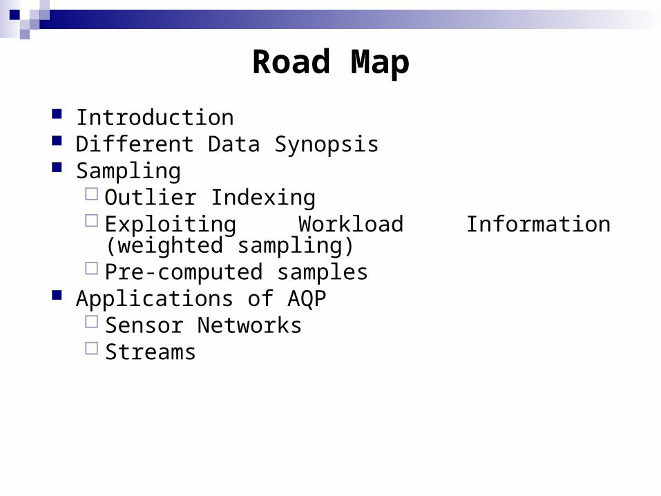
Introduction Different Data Synopsis Sampling

Outlier Indexing Exploiting Workload Information (weighted

sampling) Pre-computed samples

Applications of AQP Sensor Networks Streams

Introduction

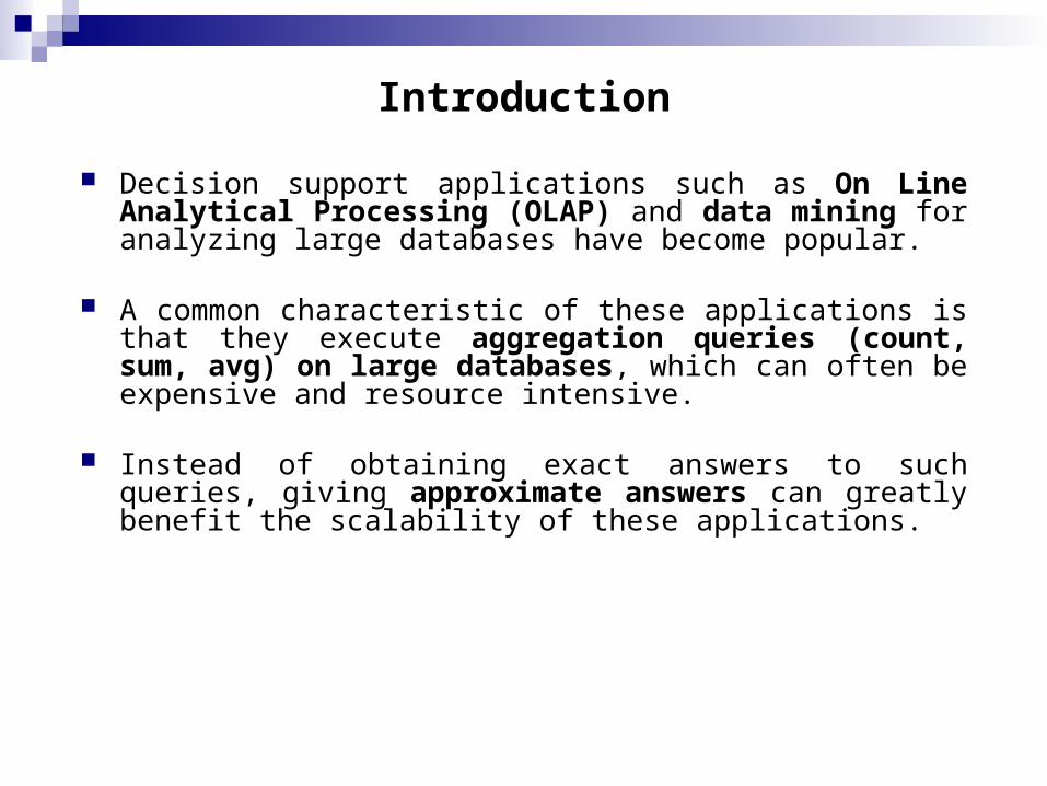
Decision support applications such as On Line Analytical Processing (OLAP) and data mining for analyzing large databases have become popular.

A common characteristic of these applications is that they execute aggregation queries (count, sum, avg) on large databases, which can often be expensive and resource intensive.

Instead of obtaining exact answers to such queries, giving approximate answers can greatly benefit the scalability of these applications.

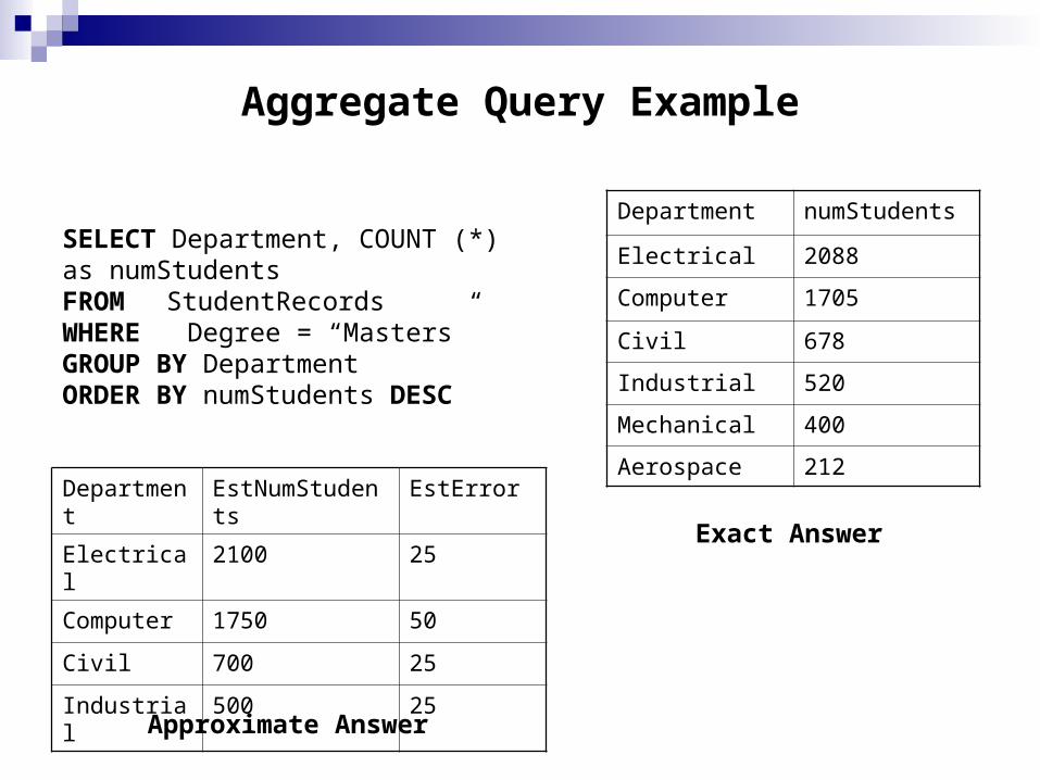
Aggregate Query Example

Department numStudents

Electrical 2088

Computer 1705

Civil 678

Industrial 520

Mechanical 400

Aerospace 212

SELECT Department, COUNT (*) as numStudentsFROM StudentRecords WHERE Degree = “Masters”GROUP BY DepartmentORDER BY numStudents DESC

Department EstNumStudents EstError

Electrical 2100 25

Computer 1750 50

Civil 700 25

Industrial 500 25

Exact Answer

Approximate Answer

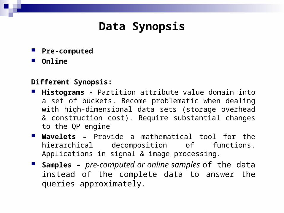
Data Synopsis

Pre-computed Online

Different Synopsis: Histograms - Partition attribute value domain into a set of buckets.

Become problematic when dealing with high-dimensional data sets (storage overhead & construction cost). Require substantial changes to the QP engine

Wavelets – Provide a mathematical tool for the hierarchical decomposition of functions. Applications in signal & image processing.

Samples – pre-computed or online samples of the data instead of the complete data to answer the queries approximately.

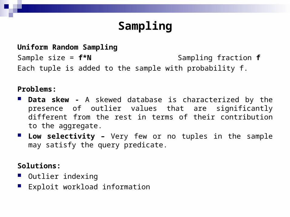
Sampling

Uniform Random Sampling

Sample size = f*N Sampling fraction f

Each tuple is added to the sample with probability f.

Problems: Data skew - A skewed database is characterized by the presence of outlier

values that are significantly different from the rest in terms of their contribution to the aggregate.

Low selectivity – Very few or no tuples in the sample may satisfy the query predicate.

Solutions: Outlier indexing Exploit workload information

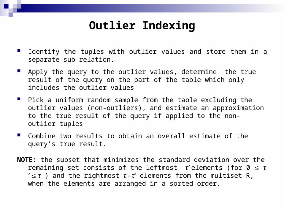
Identify the tuples with outlier values and store them in a separate sub-relation.

Apply the query to the outlier values, determine the true result of the query on the part of the table which only includes the outlier values

Pick a uniform random sample from the table excluding the outlier values (non-outliers), and estimate an approximation to the true result of the query if applied to the non-outlier tuples

Combine two results to obtain an overall estimate of the query’s true result.

NOTE: the subset that minimizes the standard deviation over the remaining set consists of the leftmost τ′ elements (for 0 τ′ τ ) and the rightmost τ - τ′ elements from the multiset R, when the elements are arranged in a sorted order.

Outlier Indexing

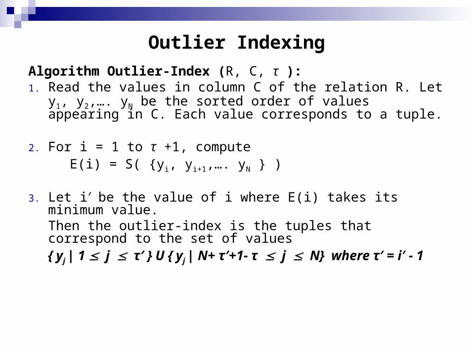
Algorithm Outlier-Index (R, C, τ ):1. Read the values in column C of the relation R. Let y1, y2,…. yN be

the sorted order of values appearing in C. Each value corresponds to a tuple.

2. For i = 1 to τ +1, computeE(i) = S( {yi, yi+1,…. yN } )

3. Let i′ be the value of i where E(i) takes its minimum value. Then the outlier-index is the tuples that correspond to the set of values { yj | 1 j τ′ } U { yj | N+ τ′+1- τ j N} where τ′ = i′ - 1

Outlier Indexing

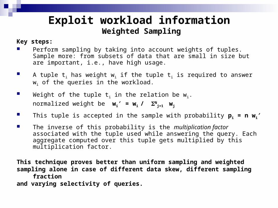
Key steps: Perform sampling by taking into account weights of tuples. Sample more:

from subsets of data that are small in size but are important, i.e., have high usage.

A tuple ti has weight wi if the tuple ti is required to answer wi of the queries in the workload.

Weight of the tuple ti in the relation be wi.

normalized weight be wi′ = wi / Nj=1

wj

This tuple is accepted in the sample with probability pi = n wi′

The inverse of this probability is the multiplication factor associated with the tuple used while answering the query. Each aggregate computed over this tuple gets multiplied by this multiplication factor.

This technique proves better than uniform sampling and weightedsampling alone in case of different data skew, different sampling fractionand varying selectivity of queries.

Exploit workload information Weighted Sampling

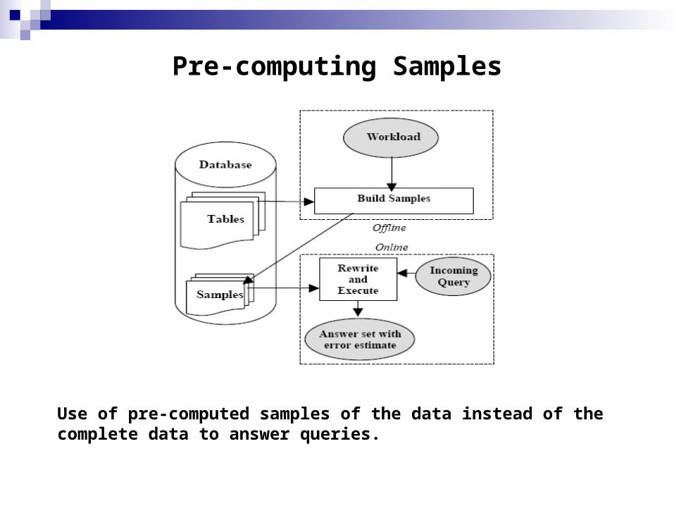
Pre-computing Samples

Use of pre-computed samples of the data instead of the complete data to answer queries.

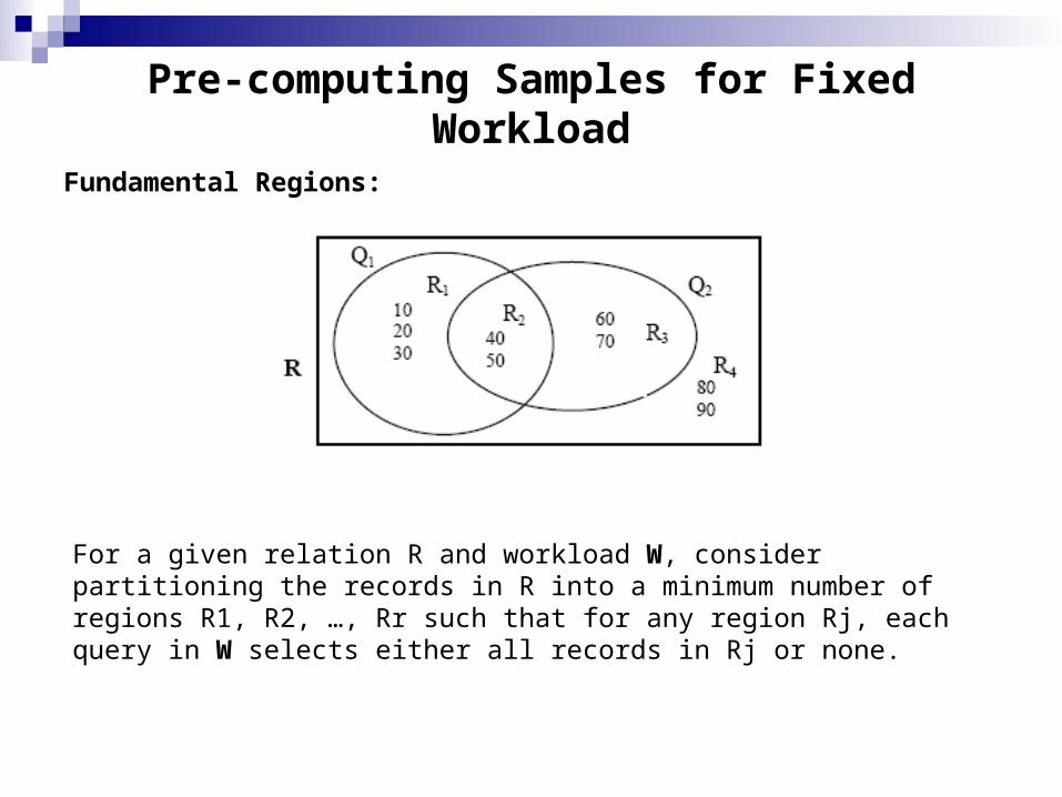
Fundamental Regions:

Pre-computing Samples for Fixed Workload

For a given relation R and workload W, consider partitioning the records in R into a minimum number of regions R1, R2, …, Rr such that for any region Rj, each query in W selects either all records in Rj or none.

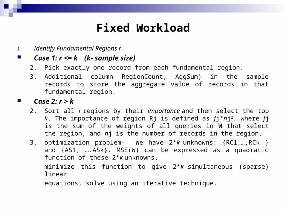
1. Identify Fundamental Regions r Case 1: r <= k (k- sample size)

2. Pick exactly one record from each fundamental region.

3. Additional column RegionCount, AggSum) in the sample records to store the aggregate value of records in that fundamental region.

Case 2: r > k2. Sort all r regions by their importance and then select the top k. The

importance of region Rj is defined as fj*nj2, where fj is the sum of the weights of all queries in W that select the region, and nj is the number of records in the region.

3. optimization problem- We have 2*k unknowns: {RC1,…,RCk } and {AS1, ….ASk}. MSE(W) can be expressed as a quadratic function of these 2*k unknowns.

minimize this function to give 2*k simultaneous (sparse) linear

equations, solve using an iterative technique.

Fixed Workload

Applications of AQP

Sensor Networks Streams

AQP in Sensor Networks

A Sensor Network is a cluster of sensor motes, devices with measurement, communication and computation capabilities, powered by a small battery.

In a typical sensor network, each sensor produces a stream of sensory observations across one or more sensing modalities.

Need for data aggregation:

unnecessary for each sensor to report its entire data stream in full fidelity. in a resource constrained sensor network environment, each message

transmission is a significant, energy-expending operation. individual readings may be noisy or unavailable.

In sensor networks we need a scalable and fault tolerant querying techniqueto extract useful information from the data the sensors collect.

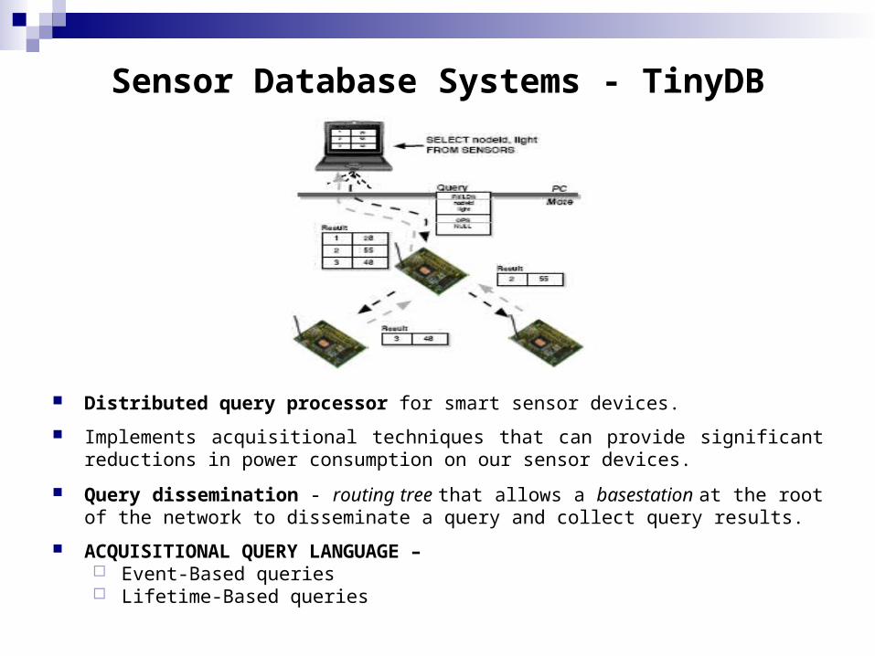
Sensor Database Systems - TinyDB

Distributed query processor for smart sensor devices.

Implements acquisitional techniques that can provide significant reductions in power consumption on our sensor devices.

Query dissemination - routing tree that allows a basestation at the root of the network to disseminate a query and collect query results.

ACQUISITIONAL QUERY LANGUAGE – Event-Based queries Lifetime-Based queries

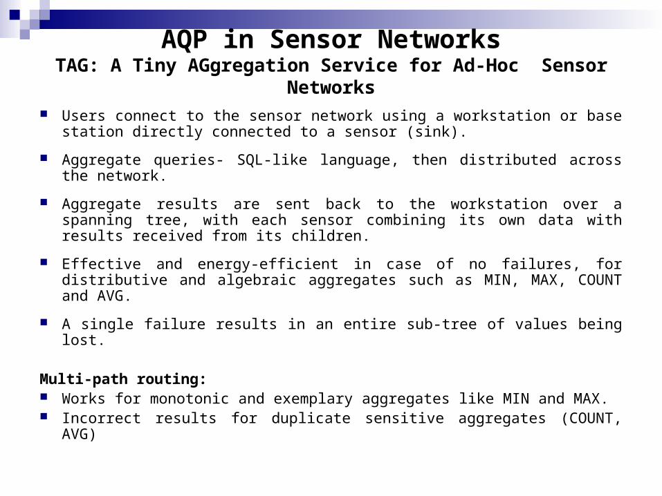
AQP in Sensor NetworksTAG: A Tiny AGgregation Service for Ad-Hoc Sensor Networks

Users connect to the sensor network using a workstation or base station directly connected to a sensor (sink).

Aggregate queries- SQL-like language, then distributed across the network.

Aggregate results are sent back to the workstation over a spanning tree, with each sensor combining its own data with results received from its children.

Effective and energy-efficient in case of no failures, for distributive and algebraic aggregates such as MIN, MAX, COUNT and AVG.

A single failure results in an entire sub-tree of values being lost.

Multi-path routing: Works for monotonic and exemplary aggregates like MIN and MAX. Incorrect results for duplicate sensitive aggregates (COUNT, AVG)

Duplicate Insensitive sketches combined with multi-path routing

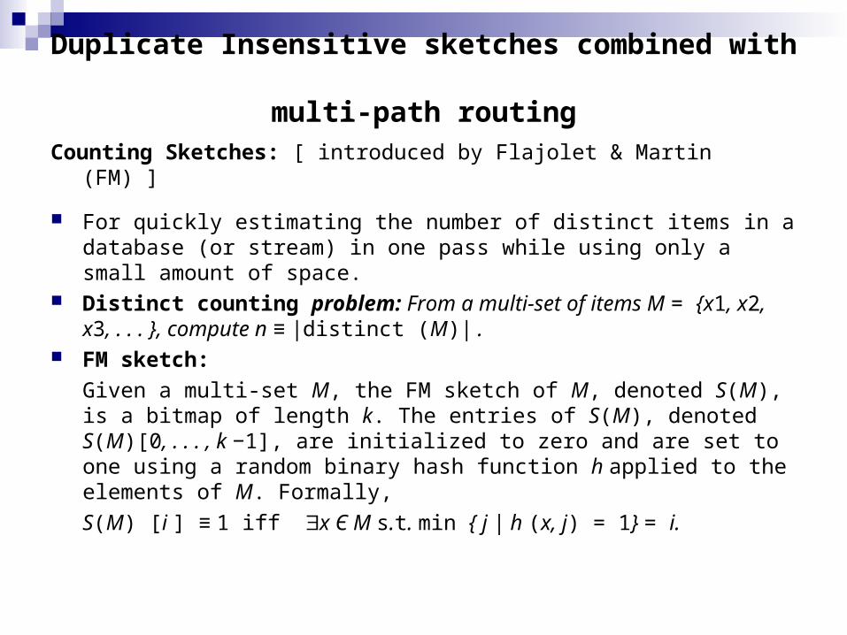
Counting Sketches: [ introduced by Flajolet & Martin (FM) ]

For quickly estimating the number of distinct items in a database (or stream) in one pass while using only a small amount of space.

Distinct counting problem: From a multi-set of items M = {x1, x2, x3, . . . }, compute n ≡ |distinct (M)| .

FM sketch:

Given a multi-set M, the FM sketch of M, denoted S(M), is a bitmap of length k. The entries of S(M), denoted S(M)[0, . . . , k −1], are initialized to zero and are set to one using a random binary hash function h applied to the elements of M. Formally,

S(M) [i ] ≡ 1 iff x Є M s.t. min { j | h (x, j) = 1} = i.


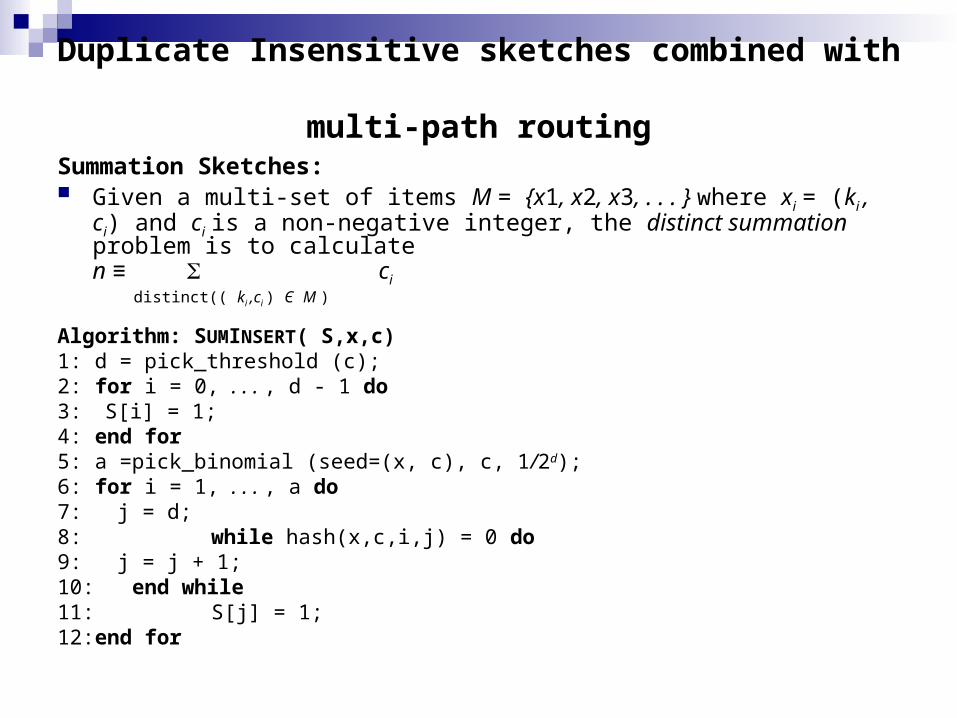
Summation Sketches: Given a multi-set of items M = {x1, x2, x3, . . . } where xi = (ki , ci) and ci is a

non-negative integer, the distinct summation problem is to calculaten ≡ ci

distinct(( ki ,ci ) Є M )

Algorithm: SUMINSERT( S,x,c)1: d = pick_threshold (c);2: for i = 0, . . . , d - 1 do3: S[i] = 1;4: end for5: a =pick_binomial (seed=(x, c), c, 1/2d);6: for i = 1, . . . , a do7: j = d;8: while hash(x,c,i,j) = 0 do9: j = j + 1;10: end while11: S[j] = 1;12:end for


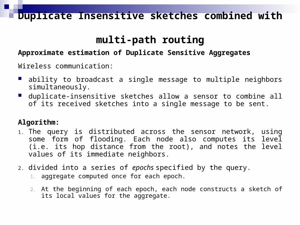
Approximate estimation of Duplicate Sensitive Aggregates

Wireless communication:

ability to broadcast a single message to multiple neighbors simultaneously. duplicate-insensitive sketches allow a sensor to combine all of its received

sketches into a single message to be sent.

Algorithm:1. The query is distributed across the sensor network, using some form of

flooding. Each node also computes its level (i.e. its hop distance from the root), and notes the level values of its immediate neighbors.

2. divided into a series of epochs specified by the query. 1. aggregate computed once for each epoch.

2. At the beginning of each epoch, each node constructs a sketch of its local values for the aggregate.


Phase 2 (cont.)3. The epoch is then sub-divided into a series of rounds, one for each level,

starting with the highest (farthest) level. 4. In each round, the nodes at the corresponding level broadcast their sketches,

and the nodes at the next level receive these sketches and combine them with their sketches in progress.

5. In the last round, the sink receives the sketches of its neighbors, and combines them to produce the final aggregate.


Analysis:

Main advantage of synchronization and rounds- better scheduling and reduced power consumption.

Loosening the synchronization increases the robustness of the final aggregate as paths taking more hops are used to route around failures.

Increased robustness comes at the cost of power consumption, since nodes broadcast and receive more often (due to values arriving later than expected) and increased time (and variability) to compute the final aggregate.

Simple gossip-based protocols(AQP in Sensor Networks cont.)

We have seen that distributed systems prove efficient over centralized ones, but with distributed systems we have instability arising due to node and link failures.

Sensor networks often involve the deployment in inhospitable or inaccessible areas that are naturally under high stress (for example in battlefields or inside larger devices).

Individual sensors may fail at any time, and the wireless network that connects them is highly unreliable.

Decentralized gossip-based protocols provide a simple and scalable solution for such highly volatile systems along with fault-tolerant information dissemination.

Due to the large scale of the system, the values of aggregate functions over the data in the whole network (or a large part of it) are often more important than individual data at nodes.

Analysis of simple gossip-based protocols(AQP in Sensor Networks cont.)

In a network of n nodes, each node i holds a value xi (or a set Mi of values).

The idea is to compute some aggregate function of these values (such as sums, averages,etc.) in a decentralized and fault-tolerant fashion, while using small messages only.

In gossip-based protocols, each node contacts one or a few nodes in each round (usually chosen at random), and exchanges information with these nodes.

Information spread resembles the spread of an epidemic.


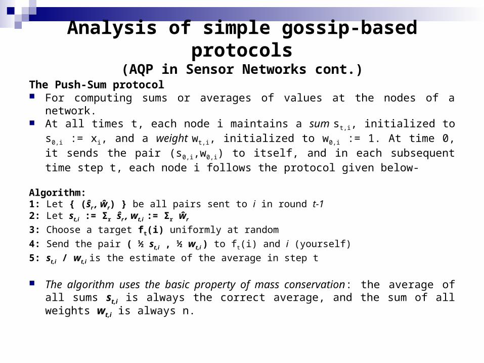
The Push-Sum protocol For computing sums or averages of values at the nodes of a network. At all times t, each node i maintains a sum st,i, initialized to s0,i := xi, and a

weight wt,i, initialized to w0,i := 1. At time 0, it sends the pair (s0,i,w0,i) to itself, and in each subsequent time step t, each node i follows the protocol given below-

Algorithm: 1: Let { (ŝr , ŵr) } be all pairs sent to i in round t-12: Let st,i := Σr ŝr , wt,i := Σr ŵr

3: Choose a target ft(i) uniformly at random

4: Send the pair ( ½ st,i , ½ wt,i ) to ft(i) and i (yourself)

5: st,i / wt,i is the estimate of the average in step t

The algorithm uses the basic property of mass conservation: the average of all sums st,i is always the correct average, and the sum of all weights wt,i is always n.


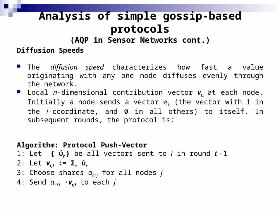
Diffusion Speeds

The diffusion speed characterizes how fast a value originating with any one node diffuses evenly through the network.

Local n-dimensional contribution vector vt,i at each node. Initially a node sends a vector ei (the vector with 1 in the i-coordinate, and 0 in all others) to itself. In subsequent rounds, the protocol is:

Algorithm: Protocol Push-Vector1: Let { ύr } be all vectors sent to i in round t -12: Let vt,i := Σr ύr

3: Choose shares αt,i,j for all nodes j4: Send αt,i,j ·vt,i to each j


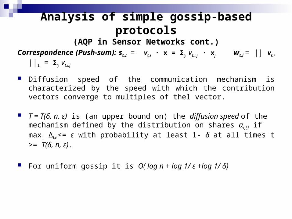
Correspondence (Push-sum): st,I = vt,i · x = Σj vt,i,j · xj wt,i = || vt,i ||1 = Σj vt,i,j

Diffusion speed of the communication mechanism is characterized by the speed with which the contribution vectors converge to multiples of the1 vector.

T = T(δ, n, ε) is (an upper bound on) the diffusion speed of the mechanism defined by the distribution on shares αt,i,j if maxi Δi,t <= ε with probability at least 1- δ at all times t >= T(δ, n, ε).

For uniform gossip it is O( log n + log 1/ ε +log 1/ δ)


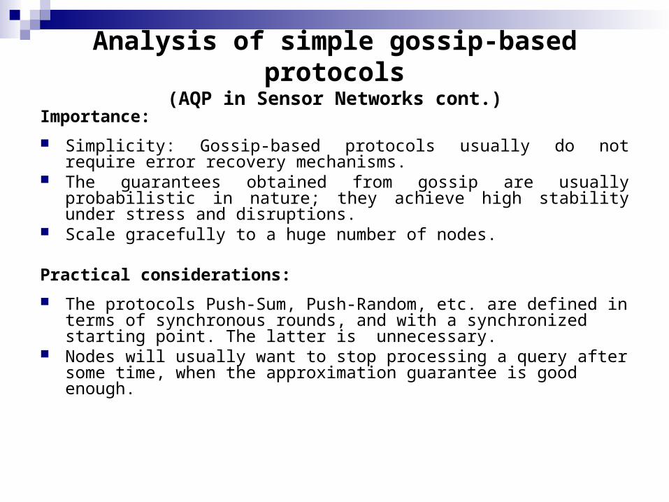
Importance:

Simplicity: Gossip-based protocols usually do not require error recovery mechanisms.

The guarantees obtained from gossip are usually probabilistic in nature; they achieve high stability under stress and disruptions.

Scale gracefully to a huge number of nodes.

Practical considerations:

The protocols Push-Sum, Push-Random, etc. are defined in terms of synchronous rounds, and with a synchronized starting point. The latter is unnecessary.

Nodes will usually want to stop processing a query after some time, when the approximation guarantee is good enough.

Approximate Query processing in Streams

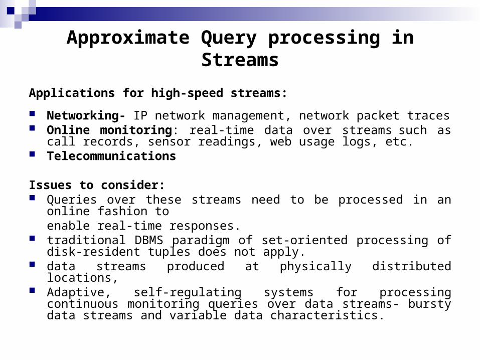
Applications for high-speed streams:

Networking- IP network management, network packet traces Online monitoring: real-time data over streams such as call records,

sensor readings, web usage logs, etc. Telecommunications

Issues to consider: Queries over these streams need to be processed in an online fashion to

enable real-time responses. traditional DBMS paradigm of set-oriented processing of disk-resident tuples

does not apply. data streams produced at physically distributed locations, Adaptive, self-regulating systems for processing continuous monitoring

queries over data streams- bursty data streams and variable data characteristics.

Adaptivity via Load Shedding Approximate Query processing in Streams (cont.)

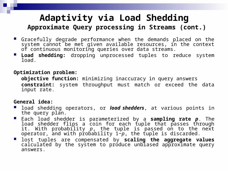
Gracefully degrade performance when the demands placed on the system cannot be met given available resources, in the context of continuous monitoring queries over data streams.

Load shedding: dropping unprocessed tuples to reduce system load.

Optimization problem:objective function: minimizing inaccuracy in query answersconstraint: system throughput must match or exceed the data input rate.

General idea: load shedding operators, or load shedders, at various points in the query

plan. Each load shedder is parameterized by a sampling rate p. The load

shedder flips a coin for each tuple that passes through it. With probability p, the tuple is passed on to the next operator, and with probability 1−p, the tuple is discarded.

lost tuples are compensated by scaling the aggregate values calculated by the system to produce unbiased approximate query answers.


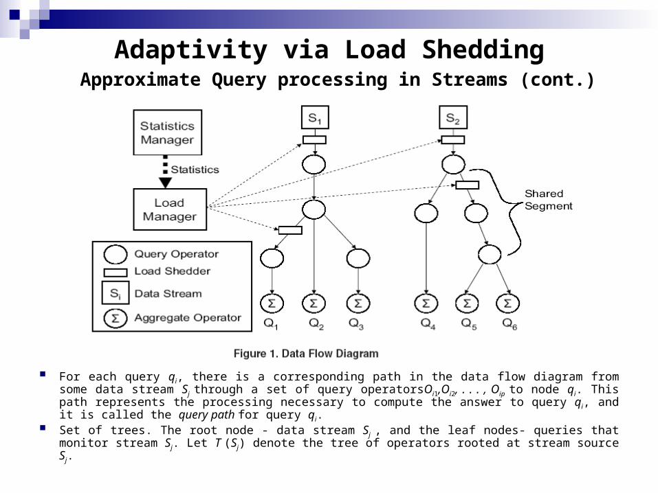
For each query qi, there is a corresponding path in the data flow diagram from some data stream Sj through a set of query operatorsOi1,Oi2, . . . , Oip to node qi. This path represents the processing necessary to compute the answer to query qi, and it is called the query path for query qi.

Set of trees. The root node - data stream Sj , and the leaf nodes- queries that monitor stream Sj. Let T (Sj) denote the tree of operators rooted at stream source Sj.


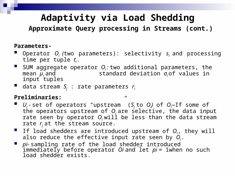
Parameters- Operator Oi (two parameters): selectivity si and processing time per tuple ti. SUM aggregate operator Oi : two additional parameters, the mean µi and

standard deviation σi of values in input tuples

data stream Sj : rate parameters ri

Preliminaries: Ui - set of operators “upstream” (Sj to Oi) of Oi—If some of the operators

upstream of Oi are selective, the data input rate seen by operator Oi will be less than the data stream rate rj at the stream source.

If load shedders are introduced upstream of Oi, they will also reduce the effective input rate seen by Oi.

pi- sampling rate of the load shedder introduced immediately before operator Oi and let pi = 1when no such load shedder exists.


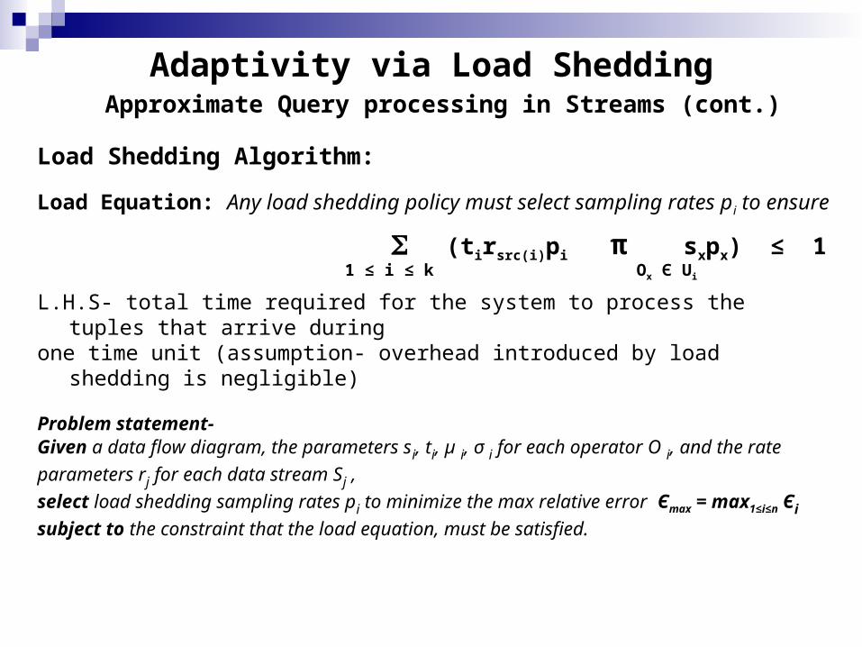
Load Shedding Algorithm:

Load Equation: Any load shedding policy must select sampling rates pi to ensure

(tirsrc(i)pi π sxpx) ≤ 1 1 ≤ i ≤ k Ox Є Ui

L.H.S- total time required for the system to process the tuples that arrive duringone time unit (assumption- overhead introduced by load shedding is negligible)

Problem statement- Given a data flow diagram, the parameters si, ti, µ i, σ i for each operator O i, and the rate

parameters rj for each data stream Sj ,

select load shedding sampling rates pi to minimize the max relative error Єmax = max1≤i≤n Єi

subject to the constraint that the load equation, must be satisfied.


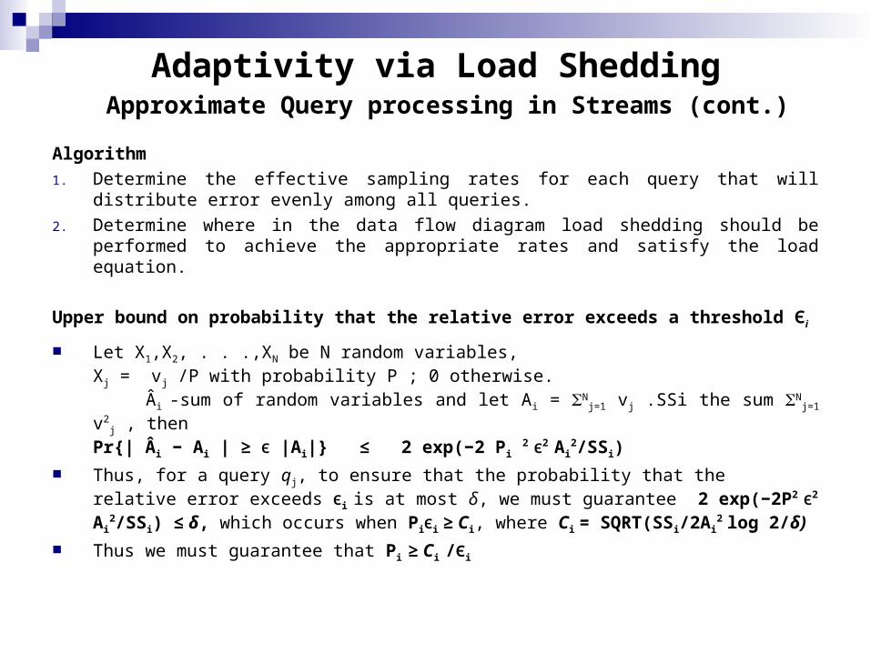
Algorithm

1. Determine the effective sampling rates for each query that will distribute error evenly among all queries.

2. Determine where in the data flow diagram load shedding should be performed to achieve the appropriate rates and satisfy the load equation.

Upper bound on probability that the relative error exceeds a threshold Єi

Let X1,X2, . . .,XN be N random variables, Xj = vj /P with probability P ; 0 otherwise.

Âi -sum of random variables and let Ai = Nj=1 vj .SSi the sum N

j=1 v2j , then

Pr{| Âi − Ai | ≥ Є |Ai|} ≤ 2 exp(−2 Pi 2 Є2 Ai

2/SSi)

Thus, for a query qj, to ensure that the probability that the relative error exceeds Єi is at most δ, we must guarantee 2 exp(−2P2 Є2 Ai

2/SSi) ≤ δ, which occurs when PiЄi ≥ Ci, where Ci = SQRT(SSi/2Ai

2 log 2/δ)

Thus we must guarantee that Pi ≥ Ci /Єi


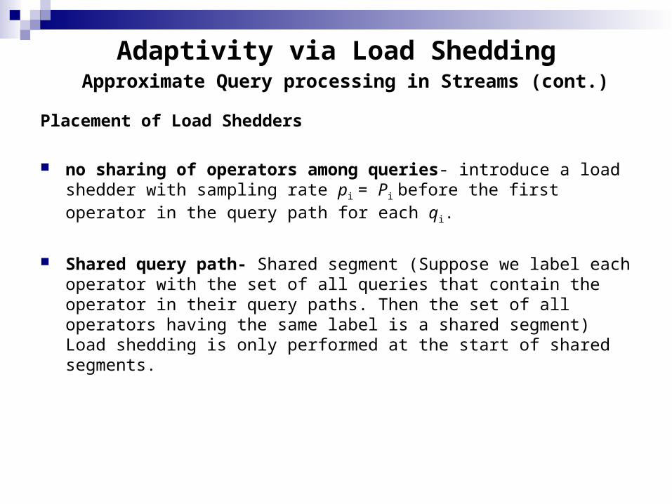
Placement of Load Shedders

no sharing of operators among queries- introduce a load shedder with sampling rate pi = Pi before the first operator in the query path for each qi.

Shared query path- Shared segment (Suppose we label each operator with the set of all queries that contain the operator in their query paths. Then the set of all operators having the same label is a shared segment) Load shedding is only performed at the start of shared segments.


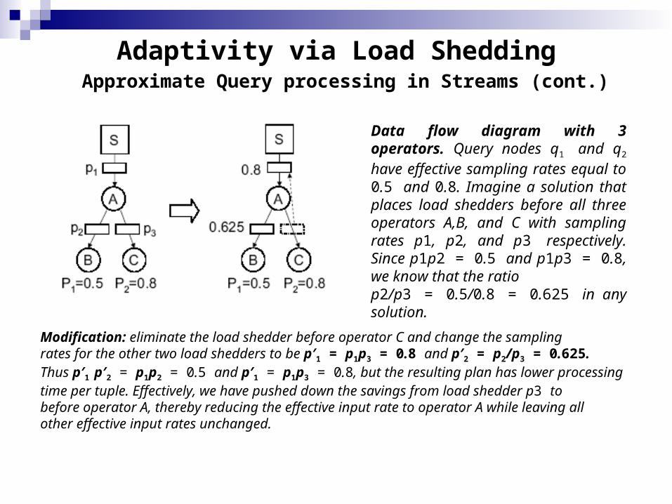
Modification: eliminate the load shedder before operator C and change the samplingrates for the other two load shedders to be p′1 = p1p3 = 0.8 and p′2 = p2/p3 = 0.625. Thus p′1 p′2 = p1p2 = 0.5 and p′1 = p1p3 = 0.8, but the resulting plan has lower processingtime per tuple. Effectively, we have pushed down the savings from load shedder p3 tobefore operator A, thereby reducing the effective input rate to operator A while leaving allother effective input rates unchanged.

Data flow diagram with 3 operators. Query nodes q1 and q2 have effective sampling rates equal to 0.5 and 0.8. Imagine a solution that places load shedders before all three operators A,B, and C with sampling rates p1, p2, and p3 respectively. Since p1p2 = 0.5 and p1p3 = 0.8, we know that the ratiop2/p3 = 0.5/0.8 = 0.625 in any solution.


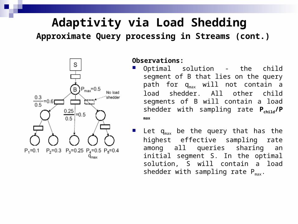
Observations: Optimal solution - the child segment of B that

lies on the query path for qmax will not contain a load shedder. All other child segments of B will contain a load shedder with sampling rate Pchild/P max

Let qmax be the query that has the highest effective sampling rate among all queries sharing an initial segment S. In the optimal solution, S will contain a load shedder with sampling rate Pmax.


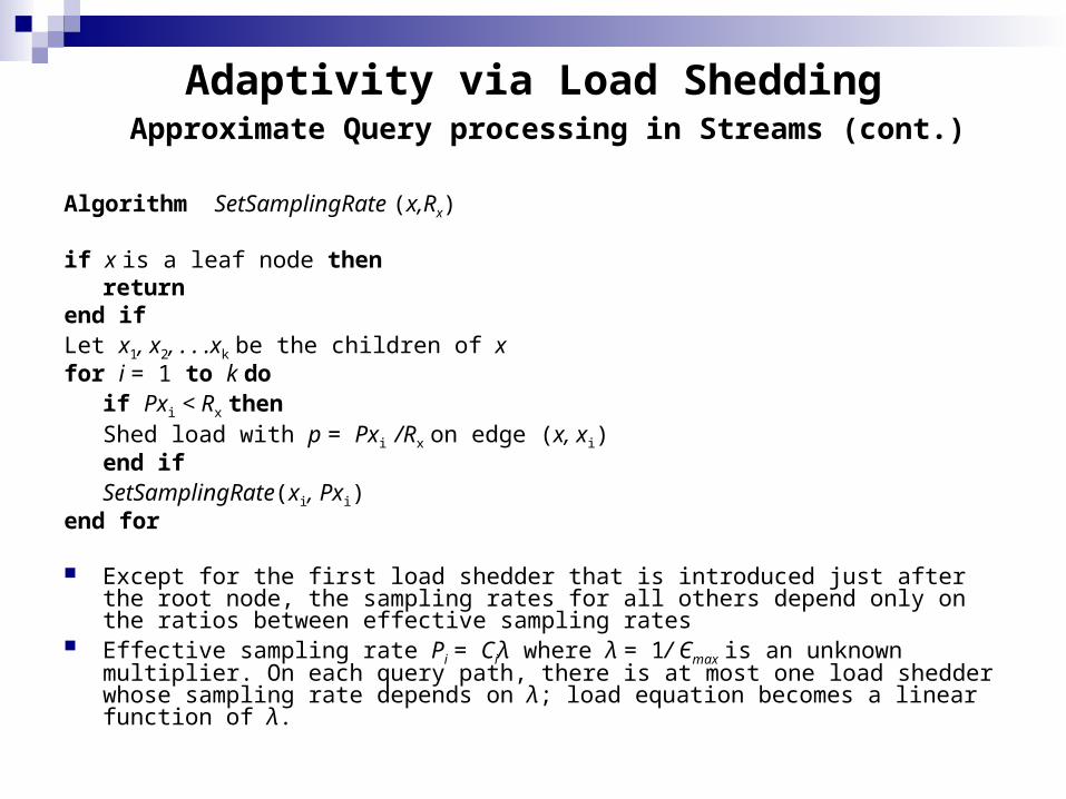
Algorithm SetSamplingRate (x,Rx)

if x is a leaf node thenreturn

end ifLet x1, x2, . . .xk be the children of xfor i = 1 to k do

if Pxi < Rx thenShed load with p = Pxi /Rx on edge (x, xi)

end ifSetSamplingRate(xi, Pxi)

end for

Except for the first load shedder that is introduced just after the root node, the sampling rates for all others depend only on the ratios between effective sampling rates

Effective sampling rate Pi = Ciλ where λ = 1/ Єmax is an unknown multiplier. On each query path, there is at most one load shedder whose sampling rate depends on λ; load equation becomes a linear function of λ.


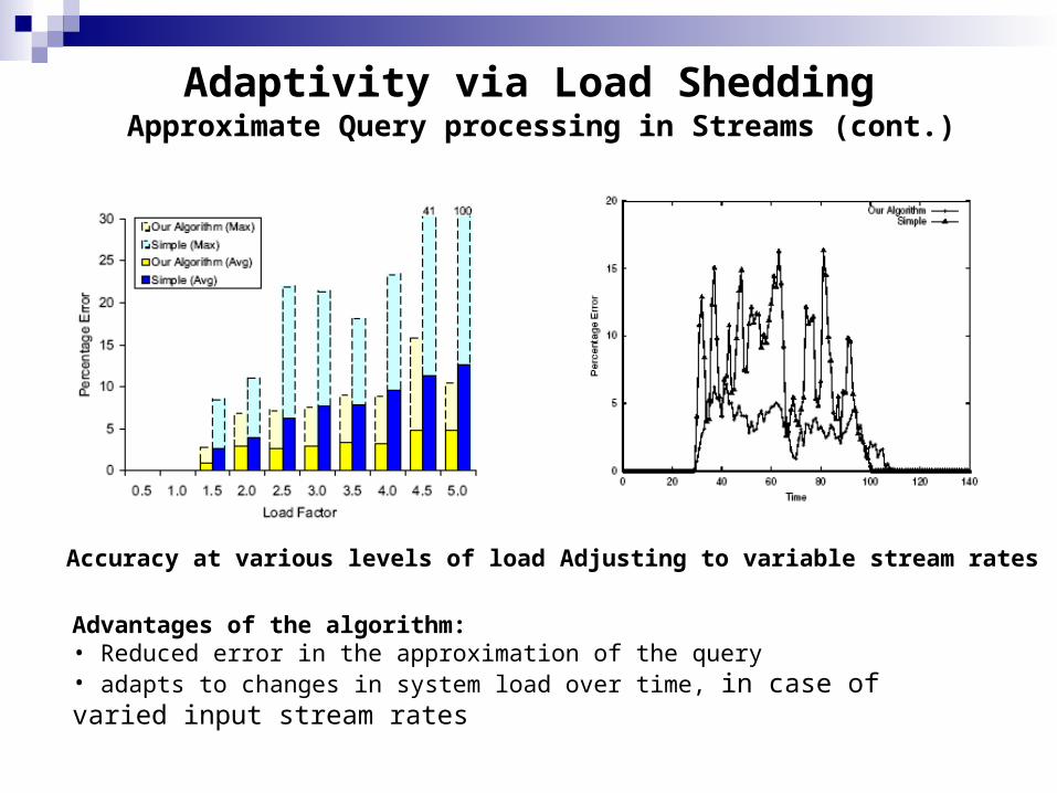
Accuracy at various levels of load Adjusting to variable stream rates

Advantages of the algorithm:• Reduced error in the approximation of the query• adapts to changes in system load over time, in case of varied input stream rates

References1. Surajit Chaudhuri, Gautam Das, Mayur Datar, Rajeev Motwani, Vivek Narasayya:

Overcoming Limitations of Sampling for Aggregation Queries. ICDE 2001. 2. Surajit Chaudhuri, Gautam Das, Vivek Narasayya: A Robust, Optimization-Based

Approach for Approximate Answering of Aggregate Queries. SIGMOD Conference 2001.

3. The design of an acquisitional query processor for sensor networks Samuel Madden, Michael J. Franklin, Joseph M. Hellerstein, Wei Hong June 2003 Proceedings of the 2003 ACM SIGMOD international conference on Management of data.

4. Approximate aggregation techniques for sensor databasesConsidine,J.;Li,F.;Kollios,G.;Byers,J.; Data Engineering, 2004. Proceedings. 20th International Conference on , 30 March-2 April 2004

5. Gossip-based computation of aggregate informationKempe,D.;Dobra,A.;Gehrke,J.; Foundations of Computer Science, 2003. Proceedings. 44th Annual IEEE Symposium on , 11-14 Oct. 2003

6. Load shedding for aggregation queries over data streamsBabcock,B.;Datar,M.;Motwani,R.; Data Engineering, 2004. Proceedings. 20th International Conference on , 30 March-2 April 2004

7. Samuel R. Madden, Michael J. Franklin, Joseph M. Hellerstein, and Wei Hong. TAG: a Tiny AGgregation Service for Ad-Hoc Sensor Networks. OSDI, December, 2002.

8. Gautam Das: Survey of Approximate Query Processing Techniques. (Invited Tutorial) SSDBM 2003

Documents

Approximate Query Processing: Techniques & Applications Presented by- Shraddha Rumade