Embed Size (px)
Citation preview

Approximate XML Joins
Huang-Chun Yu
Li Xu

Introduction
• XML is widely used to integrate data from different sources.
• Perform join operation for XML documents:– Two documents may convey approximately
or exactly the same information but may be different on structure.
– Even when two documents have the same DTD, the structures may be different due to optional elements or attributes.
Introduction
• Example:
paper
conference title authors
VLDB XML for the masses
author author
Alice Bob
paper
conference title authors
VLDB XML for the masses
author
Alice
publication
type title
conference XML for the masses
name name
Alice RobVLDB
author author
We need approximately matching of XML documents!
Introduction
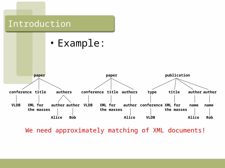
• We also need a distance metric to quantify the differences between XML documents.
• Tree edit distance is used in this paper for its generality and simplicity when quantifying the distance between trees.
• Other distance metrics can be used as well.

Tree Edit Distance
• Tree edit distance: the minimum number of tree edit operations (node insertion, deletion, label substitution) required to transform one tree to another.
• Given two trees T1 and T2, there is a well known algorithm to compute the tree edit distance in O(|T1| |T2| h(T1) h(T2)).

Tree Edit Distance
• Find a mapping M between T1 and T2 such that the editing cost is minimized.
• The mapping consists pairs of integers (i, j) such that:– 1≤ i ≤ |T1| and 1≤ j ≤ |T2|– For any (i1, j1), (i2, j2) in M
• i1 = i2 iff j1 = j2
• t1[i1] is to the left of t1[i2] iff t2[j1] is to the left of t2[j2] (sibling order preserving)
• t1[i1] is an ancestor of t1[i2] iff t2[j1] is an ancestor of t2[j2] (ancestor order preserving)

Tree Edit Distance
• Example: tree edit distance is 3 (delete B, insert H, relabel C to I)
A
B C
D E F G
A
D H
E I
F G
T1: T2:
B H

Problem Definition
• Given two XML data source S1 and S2, and a distance threshold τ.
• TDist(d1, d2): a function that assesses the tree edit distance between two documents d1 S1 and d2 S2.
• Approximate join: return all pairs of documents (d1, d2) S1 S2 such that TDist(d1, d2) ≤ τ.
Challenges
• Evaluation of TDist function between two documents is a very expensive operation. (worst case: O(n4), for trees of size O(n) )
• Traditional techniques in join algorithms (sort merge, hash join, etc) cannot be used.

Lower Bounds
• Let T be an ordered labeled tree. Let pre(T) denote the preorder traversal of T and post(T) denote the postorder traversal of T.
• Let T1, T2 be ordered labeled trees.
max{ed(pre(T1), pre(T2)), ed(post(T1), post(T2)} ≤ TDist(T1, T2)
• This can be computed in O(n2) time.

Upper Bounds
• Additional constraint is imposed on the original TDist algorithm. The search space is reduced and a faster algorithm is proposed.
• For any triple (t1[i1], t2[j1]), (t1[i2], t2[j2]), (t1[i3], t2[j3]) M, let lca( ) be the lowest common ancestor function.– t1[lca(t1[i1], t1[i2])] is a proper ancestor of t1[i3] iff
t2[lca(t2[j1], t2[j2])] is a proper ancestor of t2[j3]
• Two distinct subtrees of T1 will be mapped to two distinct subtrees of T2 .
• It can be calculated in O(|T1||T2|) time.

Upper Bounds
• Example: the upper bound is 5 (delete B, delete E, insert H, insert E, relabel C to I )
A
B C
D E F G
A
D H
E I
F G
T1: T2:

Upper Bounds
Algorithm for Upper Bound:

Outline
• Reference set
• Choosing reference set
• Approximate join algorithms

Outline
• Reference set
• Choosing reference set
• Approximate join algorithms

Reference Set
• S1, S2: two sets of XML documents
• Reference set K S1∪S2
– a chosen set of XML documents
• vi: a vector for document di S1∪S2
– dimensionality = |K|
– vit = TDist(di, kt), kt K, 1 ≤ t ≤ |K|

Reference Set
• | vit - vjt | ≤ TDist(di, dj) ≤ vit + vjt , 1 ≤ t ≤ |K|
– Essentially the above procedure “projects” documents di , dj onto the reference set K
• τ : distance threshold
• uij = min t,1 ≤ t ≤ |k| vit + vjt
– uij ≤ τ : the pair is certainly within distance τ
• lij = max t,1 ≤ t ≤ |k| |vit – vjt|
– lij > τ : the pair can’t be within distance τ

Outline
• Reference set
• Choosing reference set
• Approximate join algorithms
Choosing Reference Set
• S = S1∪S2
• S is well separated, if – S can be divided into k clusters s.t.
• Documents within a cluster have small distance (say less than τ/2)
• Documents in different clusters have large distance (say larger than 3τ/2)
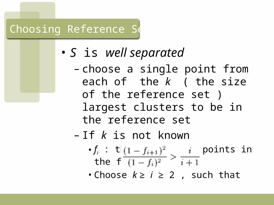
Choosing Reference Set
• S is well separated– choose a single point from each of the k
( the size of the reference set ) largest clusters to be in the reference set
– If k is not known• fi : the fraction of points in the first i clusters
• Choose k ≥ i ≥ 2 , such that
Choosing Reference Set
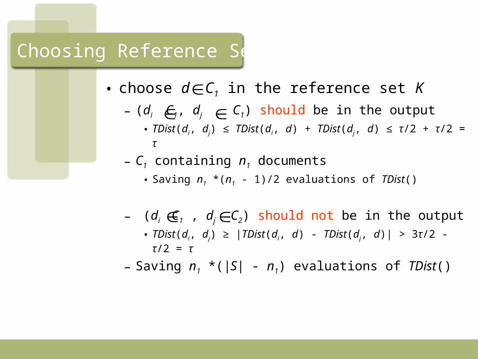
• choose d C1 in the reference set K
– (di C1, dj C1) should be in the output
• TDist(di, dj) ≤ TDist(di, d) + TDist(dj, d) ≤ τ/2 + τ/2 = τ
– C1 containing n1 documents
• Saving n1 *(n1 - 1)/2 evaluations of TDist()
– (di C1 , dj C2) should not be in the output
• TDist(di, dj) ≥ |TDist(di, d) - TDist(dj, d)| > 3τ/2 - τ/2 = τ
– Saving n1 *(|S| - n1) evaluations of TDist()

Algorithm
1. do{ 1.1 randomly pick a point d from the data set S
1.2 put all the points within τ/2 distance with d in one cluster
} until (all documents in S belong to some cluster )2. choose the k largest clusters3. pick a random point from each cluster to be in the
reference set K

Outline
• Reference set
• Choosing reference set
• Approximate join algorithms

Bounds Algorithm
• Naïve algorithm– Nested loop join + TDist algorithm
• Bounds algorithm
for each di S1 { for each dj S2 { if (UBDist(di , dj) ≤ τ ) output (di , dj); if (LBDist(di , dj) ≤ τ ) if (TDist(di , dj ) ≤ τ ) output(di , dj); }}

Pruning with a Reference Set
• for each pair (di S1, dj S2 )
– uij = min t,1 ≤ t ≤ |k| vit + vjt
– lij = max t,1 ≤ t ≤ |k| |vit – vjt|
• uij ≤ τ : the pair belongs to the output
• lij > τ : the pair can be pruned away
• lij ≤ τ < uij : apply TDist(di, dj) to identify the distance between di and dj
• refer to this algorithm as RS (ReferenceSets)• Drawback
– need to perform (| S1| + |S2|) * |K| invocations of TDist() to compute vectors

Applying Both Optimizations
• if RS algorithm indicates that TDist() should be invoked between a pair– can be possibly avoid by applying the
computational cheaper LBDist() and UBDist()
• refer to this algorithm as RSB (RSBounds)

RSC Algorithm
• potentially more evaluation of TDist()– because of the construction of vectors
• two vectors for document di S1∪S2
– vector vli : vl
it = LBDist(di, kt), kt K, 1 ≤ t ≤ |K|
– vector vui : vu
it = UBDist(di, kt), kt K, 1 ≤ t ≤ |K|
• | vlit - v
ujt | ≤ TDist(di, dj) ≤ vu
it + vujt , 1 ≤ t ≤ |K|
• uij = min t,1 ≤ t ≤ |k| vuit + vu
jt
• lij = max t,1 ≤ t ≤ |k| |vlit – vu
jt|
• Refer to this algorithm as RSCombined(RSC)• Drawback: double the size of vectors

Performance Evaluation
• Run time vs. number of nodes
0
0.5
1
1.5
2
2.5
3
0 500 1000 1500 2000 2500 3000
Number of nodes
Run
tim
e (s
ec)
Treedist
LBound
UBound

Performance Evaluation
• Run time vs. distance threshold (XMark)
• Run time vs. distance threshold (DBLP)
140
150
160
170
180
190
200
210
0 20 40 60 80 100 120
Distance Threshold
Run
Tim
e (s
ec)
Naïve
Bound
24.5
25
25.5
26
26.5
27
0 5 10 15 20 25
Distance Threshold
Run
Tim
e (s
ec)
Naïve
Bound

Performance Evaluation
• Run time vs. distance threshold (XMark)
• Number of TDist calculation vs. distance threshold (XMark)
0
1000
2000
3000
4000
5000
6000
10 20 30 40 50 60 70 80 90 100 110
Distance Threshold
# of
TD
ist
Naïve
Bound
RS
RSB
RSC
150
200
250
300
350
400
10 20 30 40 50 60 70 80 90 100 110
Distance threshold
Run
tim
e (s
ec)
RS
RSB
RSC

Conclusion & Future Work
• The algorithms are not scalable for huge data sets.
• The performance of these algorithms has a strong correlation with the data itself.
• The performance of the reference set depends on the clustering algorithm chosen.
• Try to incorporate other distance matrices into the algorithms.
• Try to explore the various indexing schemes which can be used in the algorithms.

References
• S. Guda, H. V. Jagadish, N. Koudas, D. Srivastava, and T. Yu, Approximate XML Joins, Proceedings of ACM SIGMID, 2002.
• K. Zhang and D. Shasha, Tree Pattern Matching, Oxford University Press, 1997.
• S. Guha, R. Rastogi, and K. Shim, CURE: An Efficient Clustering Algorithm for Large Databases, Proceedings of ACM SIGMOD, 1998.
• T. Zhang, R. Ramakrishnan, and M. Livny, BIRCH: An Efficient Data Clustering Method for Very Large Databases, Proceedings of ACM SIGMOD, 1996.


![Holistic Twig Joins: Optimal XML Pattern Matching · Holistic Twig Joins: Optimal XML Pattern Matching ... A1-Khalifa et al. [1] ... and show that it is I/O and CPU optimal among](https://img.pdfslide.net/doc/110x75/5ae95f6a7f8b9a3d3b913d18/holistic-twig-joins-optimal-xml-pattern-twig-joins-optimal-xml-pattern-matching.jpg)