Approximately Optimum Stratification on the Auxiliary Variable

Approximately Optimum Stratification on the Auxiliary VariableAuthor(s): Ravindra SinghSource: Journal of the American Statistical Association, Vol. 66, No. 336 (Dec., 1971), pp. 829-833Published by: American Statistical AssociationStable URL: http://www.jstor.org/stable/2284235 .

Accessed: 14/06/2014 06:42

Your use of the JSTOR archive indicates your acceptance of the Terms & Conditions of Use, available at .http://www.jstor.org/page/info/about/policies/terms.jsp

.JSTOR is a not-for-profit service that helps scholars, researchers, and students discover, use, and build upon a wide range ofcontent in a trusted digital archive. We use information technology and tools to increase productivity and facilitate new formsof scholarship. For more information about JSTOR, please contact [email protected].

.

American Statistical Association is collaborating with JSTOR to digitize, preserve and extend access to Journalof the American Statistical Association.

http://www.jstor.org

This content downloaded from 195.34.79.101 on Sat, 14 Jun 2014 06:42:41 AMAll use subject to JSTOR Terms and Conditions

http://www.jstor.org/action/showPublisher?publisherCode=astata

http://www.jstor.org/stable/2284235?origin=JSTOR-pdf

http://www.jstor.org/page/info/about/policies/terms.jsp


?) Journal of the American Statistical Association December 1971, Volume 66, Number 336

Theory and Methods Section

Approximately Optimum Stratification on the Auxiliary Variable

RAVINDRA SINGH*

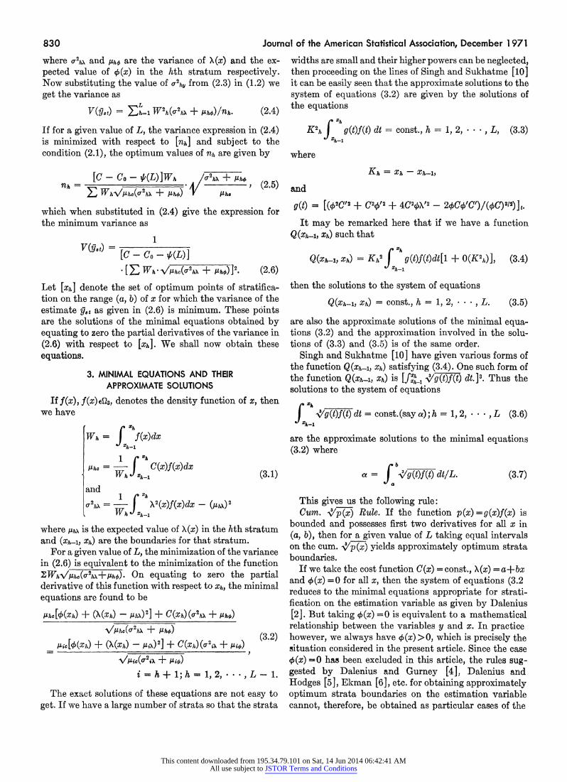
Serfing [8] has obtained optimum stratification on the auxiliary variable x making use of the cum. \/f method when the regression of the estimation variable y on x is linear and the correlation is nearly perfect. In the present article another procedure, applicable in more general situations, is suggested to obtain optimum stratification on x. The method rnakes use of a new cum. V/p(x) rule for obtaining approximately optimum strata boundaries. A priori knowledge of the form of regression of y on x and the form of the conditional variance function V(xl y) is assumed. The article concludes with a numerical example.

1. INTRODUCTION Let the population under consideration be divided into

L strata and a stratified simple random sample of size n be drawn from it, the sample size in the hth stratum being nh so that Ehnh =n. If y is the variable under study, an unbiased estimate of the population mean is given by

gat = Eh=l Whh (1.1)

where Wh is the proportion of units in the hth stratum and Yh iS the sample mean based on nh units drawn from that stratum.

Ignoring the finite population correction factors, the variance of the estimate yst is found to be

V(yst) = h1 W2hS hy/nh. (1.2)

In order to achieve maximum precision, the stratification design that minimizes V(gy8,) is desired. From (1.2) it is clear that the problem of optimum stratification in- volves the simultaneous determination of (a) optimum strata boundaries, (b) optimum number of strata and (c) the sample allocation [nhj.

The problem of determining optimum strata boundaries, when both the estimation and stratification variables are the same, was first considered by Dalenius [2]. The subsequent work in this direction is also well known. Regarding the optimum stratification on the auxiliary variable x, Dalenius [3] obtained minimal equations for Neyman allocation while Taga [11] has considered the case of proportional allocation. Subsequently Siiigh and Sukhatme [10] have obtained the minimal equations giving optimum strata boundaries on x-scale for the case of Neyman allocation (minimizing the variance for fixed

* Ravindra Singh is assistant professor of statistics, Department of Mathematics and Statistics, Panjab Agricultural University, Ludhiana, India. The author is grateful to the editors for certain helpful suggestions.

n) and have also suggested various methods of finding their approximate solutions.

Serfling [8] has used the cum. \/I method of Dalenius and Hodges [5] for obtaining optimum stratification on both the estimation and auxiliary variables. In the latter case, regression of y on x is assumed to be linear with uncorrelated homoscedastic errors and nearly perfect correlation. In the present article, assuming the a priori knowledge of the regression of y on x and also the form of conditional variance function V(y I x), a new cum. -AIp(x) rule has been suggested to obtain approximately optimum strata boundaries on the variable x. This rule has been used to obtain optimum stratification for a fixed total cost.

Before we proceed further let us define the class Qr of functions. A function d(x) is said to belong to Qr if the first r derivatives of 6(x) exist for all x in the range (a, b) of x.

2. OPTIMUM ALLOCATION Here we shall consider the question of optimum alloca-

tion of the sample to different strata when the total expected cost of the survey is fixed. As the variable x can also be treated as a size measure, let us assume that the cost of observing y on a unit is a function of the value of the variable x for that unit. If C(x) (C(x)eQ3, C(x) >0 for all x in (a, b)) is this function then the expected cost for observing nh units in the hth stratum is nh I/hc where ILhc

is the expected value of C(x) in the hth stratum. The cost function can, therefore, be taken as

C - Co + Eh=l nhI + + 1A(L), (2.1)

where CO is the overhead cost and A/(L) is the cost of con- structing L strata with Vt(1) = 0. We shall assume the total expected cost C to be fixed.

Let the regression of y on x be given by

y = X(x) + e, (2.2)

where E(ejx)-O and V(ejx) =q(x)>O for all x in the range (a, b) of x with (b -a) < oo . We also assume that X(x) IE2 while 4(x)eig. With this regression model, we have

a2hy = U2 hX + A ho, (2.3)

829



830 Journal of the American Statistical Association, December 1 971

where 2hx and Ah0 are the variance of X(x) and the expected value of b(x) in the hth stratum respectively. Now substituting the value of 2'h, from (2.3) in (1.2) we get the variance as

V(q8St) = f Wh=1 Wh(O-2hX + AhO)/nh. (2.4)

If for a given value of L, the variance expression in (2.4) is minimized with respect to [nh] and subject to the condition (2.1), the optimum values of nh are given by

_ [C - Co - /UL)W4 2hX + /.Lj -h A! V (2.5) n >2 WhV\I.h0 (o2hX + AhO Ah Vl.V

which when substituted in (2.4) give the expression for the minimum variance as

V(g8t) [C-CO-A(L)]

.[E Wh.V,hc (U2hX + AOh)]2* (2.6)

Let [xh] denote the set of optimum points of stratification on the range (a, b) of x for which the variance of the estimate ?et as given in (2.6) is minimum. These p6ints are the solutions of the minimal equations obtained by equating to zero the partial derivatives of the variance in (2.6) with respect to [xh]. We shall now obtain these equations.

3. MINIMAL EQUATIONS AND THEIR APPROXIMATE SOLUTIONS

If f(x), f(x) Ec23, denotes the density function of x, then we have f Zh

Wh = f(x)dx

1 Ac=C(x)f(x)dx

Wh = - (3.1)

and 1 Xh

a = - W X 2(x)f(x)dx - (4hX)

where IhX is the expected value of X(x) in the hth stratum and (xh-1, xh) are the boundaries for that stratum.

For a given value of L, the minimization of the variance in (2.6) is equivalent to the minimization of the function ZWhV\/Ih,(U2hX+ I.hO). On equating to zero the partial derivative of this function with respect to Xh, the minimal equations are found to be

/.hc[k(Xh) + (X(Xh) - ghX)2] + C(Xh)(02hX + /hO)

V\/lhc(2 hX + /AhO)

_ic[L(Xh) + (X(Xh) - PA)2] + C(Xh)(of2e + pli+) (3.2)

Vi=c(of2 h + Hi+)

The exact solutions of these equations are not easy to get. If we have a large number of strata so that the strata

widths are small and their higher powers can be neglected, then proceeding on the lines of Singh and Sukhatme [10] it can be easily seen that the approximate solutions to the system of equations (3.2) are given by the solutions of the equations

e Xh

K2hJg (t)f(t) dt = const., h = 1, 2, , L, (3.3)

where

Kh = Xh - Xh-l,

and

g(t) = [(02Cp'2 + C24/2 + 4C2c/A'2 - 20C0'C')/(0C)3I2)]t.

It may be remarked here that if we have a function Q(xh-1, Xh) such that

Q(xhl, Xh) = Kh f g(t)f(t)dt[1 + O(K2h)], (3.4)

then the solutions to the system of equations

Q(xh-1, Xh) = const., h = 1, 2, * * * , L. (3.5)

are also the approximate solutions of the minimal equations (3.2) and the approximation involved in the solutions of (3.3) and (3.5) is of the same order.

Singh and Sukhatme [10] have given various forms of the function Q(Xh-1, Xh) satisfying (3.4). One such form of the function Q(xh-1, Xh) is [f_ Ih <g(t)f(t) dt. ]3I Thus the solutions to the system of equations

rX' f 4Yg(t)f(t) dt = const.(say a); h = 1, 2, . . ., L (3.6) h-1

are the approximate solutions to the minimal equations (3.2) where

rb a = f </g(t)f(t) dt/L. (3.7)

This gives us the following rule: Cum. V/p(x) Rule. If the function p(x) = g(x)f(x) is

bounded and possesses first two derivatives for all x in (a, b), then for a given value of L taking equal intervals on the cum. V/p(x) yields approximately optimum strata boundaries.

If we take the cost function C(x) = const., X(x) = a+bx and +(x) =0 for all x, then the system of equations (3.2 reduces to the minimal equations appropriate for stratification on the estimation variable as given by Dalenius [2]. But taking +(x) =0 is equivalent to a mathematical relationship between the variables y and x. In practice however, we always have 4 (x) >0, which is precisely the situation considered in the present article. Since the case 4(x) -0 has been excluded in this article, the rules suggested by Dalenius and Gurney [4], Dalenius and Hodges [5], Ekman [6], etc. for obtaiiing approximately optimum strata boundaries on the estimation variable; cannot, therefore, be obtained as particular cases of the



Optimum Stratification on Auxiliary Variable 831 cum. ,/p(x) rule. This rule is, thus, different frona tie other rules proposed for obtaining approximately optimum strata boundaries on the estimation variable.

In the next section we shall express the variance V(y.) as given in (2.6) in terms of number of strata L and some other constants which do not depend on the strata boundaries.

4. THE VARIANCE V(Y8t) IFor this purpose we make use of the following lemma

due to Singh [9]. Lemma 4.1. If (Xh-l, Xh) are the boundaries of hth stra-

tum and Kh = Xh - Xh-1, then

WhVIXhc(O72hX + h - IJ V (t)C(t)f(t)dt Xh-

=6 1 [fxhS(&(t) dt [1 + 0(K2h)I (4.1)

If the terms of order 0(m5), m-sup(a,b) (Kh), are neglected we get approximately

r h

WhVlihc(a2hX + Ah0 - f V\(t)C(t)f(t) dt h-1

= \Yg(t)f(t) dt /96, (4.2)

and the value of the right-hand side of (4.2) in the points obtained by solving (3.6) (which are also the approximate solutions to the minimal equations (3.2)) is equal to

. wb -3

[fb g(t)f(t) dt /96L3 = -l/L3, (4.3)

where =- fba -/Yg(t)f(t) dt]3/96, is constant and does not change with L and the strata boundaries.

The variance of the estimate gt is, therefore, given by

V(z8s) = ( + ,/L2)/(C - Co -(L))j

where rb

= jib (t)C(t)f(t)dt. (4.4)

For calculating the values of a and y from the frequency table one could use the following approximate expressions

= [ {K2*g(x*)W,} 1I3]3/96 (4.5) and

7 = S V+(x)C(xt) Wi,

where for the ith class ti is the midvalue, K; is the width and Wi is the relative frequency and the summation is carried over all the classes.

5. OPTIMUM NUMBER OF STRATA The variance of the estimate g.t as given in (4.4) has an

approximately minimal value for the given number of

strata aad fixed total cost C. Now to obtain approximately optimum stratification it remains to firnd an optimum value for L, the number of strata to be constructed. The variance in (4.4) is only the function of L as 3 and 'y are constants for a given population and for the given choice of the auxiliary variable x.

Now it may be found without difficulty that the optimum L satisfies the differential equation

,yL'Vb'(L) + AL{P'(L) - 4,3(C - Co - VI(L)) = 0, (5.1)

where t3 and y have been defined in (4.3) and (4.4), respectively. Various particular cases can now be obtained by taking different forms for the function '(L).

Once the optimum number of strata L is determined from the equation (5.1), the system of equations (3.6) may be used for finding the approximately optimum strata boundaries.

6. APPROXIMATE EXPRESSIONS FOR [f,]

After the strata boundaries have been determined by solving the system (3.6) for the number of strata L satisfying (5.1), the sample size nh allocated to the hth stratum is given by (2.5). Since the functions f(x), C(x), X(x) and +(x) are known a priori, the parameters Wh,

lhy a2hx and 'h1 can be evaluated and the value of nh

can be determined. The total sample size n is then 2nh. It may be sometimes tedious to determine nh from the

relation (2.5) because of the integrations involved in it. We now obtain the approximate expressions for the sample size nh. For this the series expansion of WhV(aT2hx+Yh0)//1hc, in powers of Kh, is required. It is easy to verify that by proceeding on lines of proof for lemma (4.1), we obtain

XA1

K2 rXh 9 J S(t)f(t) dt[l + O(K2 h) (6.1)

where

S(t) = [(40C2XV2 - 302C12 + C24/2 + 2C44/C1)/ 3I2C5I2]t.

Therefore, if the terms of order 0(m5) are neglected, the sample size nh in the hth stratum is given by

C - Co -

(y + #/L2)

[ f CC(t) f(t) dt + 96 S(t)f(t) dt (6.2) L ~, 'VC(t) 96d]

as from (4.2) and (4.3)

L2 Eh1 WyVgsc(u2s,A + -5 + 3/L

If w^ (xs_1+xs)/2, than (6.2) is approximnately given by



832 Journal of the American Statistical Association, December 1 971

C- Co-*(L) nIh= (' + O/I2)

*[V/(xh)/C(xth) + (K2h-S(xh)/96]Wh, (6.3)

since we have for a given function u(x)

Xh ~~~~~pXh f u(t)f(t) dt U u(th)j f(t) dt[l + O(K2h)

From Lemma 4.1, it may be easily seen that the optimum cost allocated to the hth stratum is approximately equal to

C - Co - ,6(L) r (Xh (ey+ /L2) [J \v((t)C(t)(t) dt + i3/L2j. (6.4)

From (6.2) it is clear that the optimum sample allocation is not an equal allocation as we have in the case of stratification on the estimation variable.

7. NUMERICAL ILLUSTRATION

In practice we have available the frequency distribution of the auxiliary variable x. Suppose the distribution is as given in Table 1.

1. RELATIVE FREQUENCY DISTRIBUTION FOR THE VARIABLE x

Class-interval f 2/T Cum 3

(1) (2) (3) (4)

1.0 1.5 0.39347 0.73279 0.73279 1.5 - 2.0 0.23865 0.62029 1.35308 2.0 - 2.5 0.14475 0.52506 1.87814 2.5 - 3.0 0.08779 0.44462 2.32276 3.0 - 3.5 0.05326 0.37622 2.69898 3.5 - 4.0 0.03229 0.31846 3.01744 4.0 - 4.5 0.01959 0.26960 3.28704 4.5 - 5.0 0.01188 0.22829 3.51533 5.0 - 5.5 0.00721 0.19303 3.70836 5.5 - 6.0 0.00437 0.16364 3.87200

Let us assume that from a priori information we have X(x)=a+x, 0(x)=0.1 x, C(x)=10 x and V(L)=40 L. Now for determining the optimum number of strata from the equation (5.1) we must find the values of A and y from the frequency table. Using the approximations (4.5), we obtain from Table 1 3= 1.51173 and y=1.97344. If C - Co = 2,000 the equation (5.1) becomes

1.97344 L3 + 7.55865 L = 302.346.

On solving the equation, the optimum number of strata is found to be 5.

Now once the number of strata to be constructed is determined, the strata boundaries are obtained by using cum. -p(x) rule. In this particular case we have g(x) = 10 so that the cum.V/p(x) rule is reduced to cum.Vf(x) rule. Thus by taking equal intervals on the cum.-,YJin Table 1 the strata boundaries are obtained as 1.0000, 1.5335, 2.1864, 3.0051, 4.1488 and 6.0000. We then prepare the

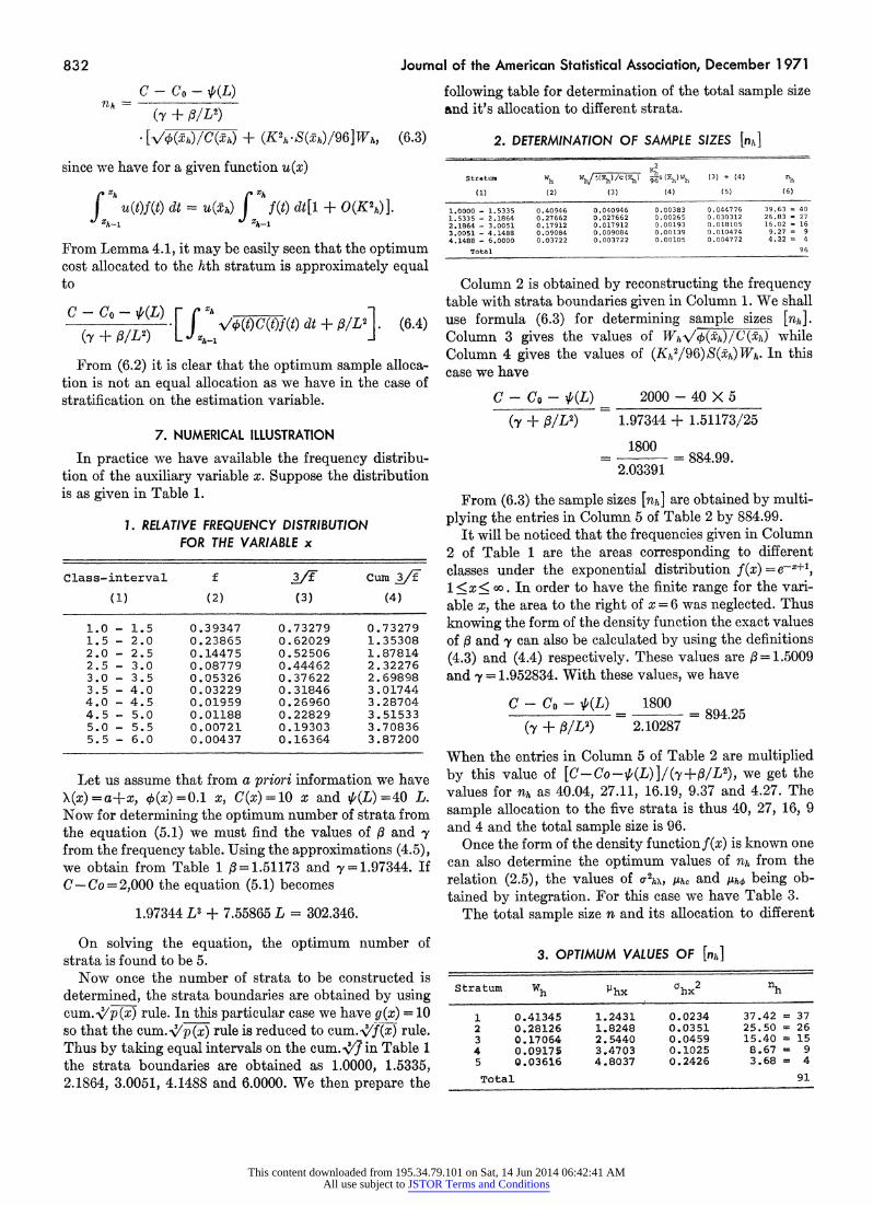
following table for determination of the total sample size and it's allocation to different strata.

2. DETERMINATION OF SAMPLE SIZES [nh]

Stratura Wh Wh (Xh)/C(Xh) gSCOh)Wh (3) + (4) nh

(1) (2) (3) (4) (5) (6)

1.0000 - 1.5335 0.40946 0.040946 0.00383 0.044776 39.63 = 40

1.5335 - 2.1864 0.27662 0.027662 0.00265 0.030312 26.83 - 27

2.1864 - 3.0051 0.17912 0.017912 0.00193 0.018105 16.02 = 16

3.0051 - 4.1488 0.09084 0.009084 0.00139 0.010474 9.27 = 9

4.1488 - 6.0000 0.03722 0.003722 0.00105 0.004772 4.22 = 4

Total 96

Column 2 is obtained by reconstructing the frequency table with strata boundaries given in Column 1. We shall use formula (6.3) for determining sample sizes [nh].

Column 3 gives the values of WhV\1(PQjh)/C(Xh) while Column 4 gives the values of (Kh2/96)S(h)WVh. In this case we have

C-Co-{(L) 2000-40 X 5

(Y + O/L2) 1.97344 + 1.51173/25

1800 -- 2.03391= 884.99.

2.03391

From (6.3) the sample sizes [nh] are obtained by multi- plying the entries in Column 5 of Table 2 by 884.99.

It will be noticed that the frequencies given in Column 2 of Table 1 are the areas corresponding to different classes under the exponential distribution f(x)=e-z+', 1 <x < oo . In order to have the finite range for the variable x, the area to the right of x = 6 was neglected. Thus knowing the form of the density function the exact values of X and y can also be calculated by using the definitions (4.3) and (4.4) respectively. These values are 13=l.5009 and 7y=1.952834. With these values, we have

C - C0 - iP(L) 1800

(e + j/LI) 2.10287

When the entries in Column 5 of Table 2 are multiplied by this value of [C-Co-4(L)]1(y+01L2), we get the values for nh as 40.04, 27.11, 16.19, 9.37 and 4.27. The sample allocation to the five strata is thus 40, 27, 16, 9 and 4 and the total sample size is 96.

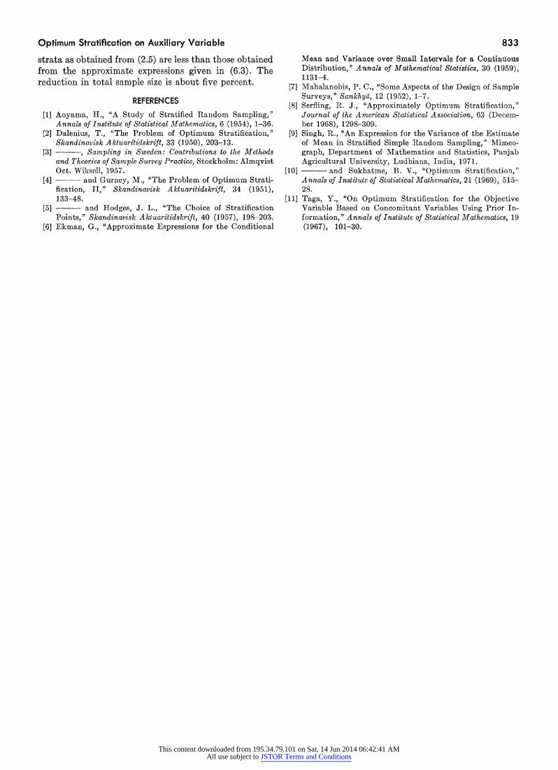
Once the form of the density function f(x) is known one can also determine the optimum values of nh from the relation (2.5), the values of o-2 , .Lhc and Aho being obtained by integration. For this case we have Table 3.

The total sample size n and its allocation to different

3. OPTIMUM VALUES OF [nh]

Stratum Wh Phx ahx2 nh

1 0.41345 1.2431 0.0234 37.42 = 37 2 0.28126 1.8248 0.0351 25.50 = 26 3 0.17064 2.5440 0.0459 15.40 = 15 4 0.09175 3.4703 0.1025 8.67 = 9 5 Q .03616 4 .8037 0.2426 3 .68 = 4 Total 91



Optimum Stratification on Auxiliary Variable 833

strata as obtained from (2.5) are less than those obtained from the approximate expressions given in (6.3). The reduction in total sample size is about five percent.

REFERENCES

[11 Aoyama, H., "A Study of Stratified Random Sampling," Annals of Institute of Statistical Mathematics, 6 (1954), 1-36.

[2] Dalenius, T., "The Problem of Optimum Stratification," Skandinavisk Aktuaritidskrift, 33 (1950), 203-13.

[3] , Sampling in Sweden: Contributions to the Methods and Theories of Sample Survey Practice, Stockholm: Almqvist Oct. Wiksell, 1957.

[4] - and Gurney, M., "The Problem of Optimum Strati- fication, II, " Skandinavisk Aktuaritidskrift, 34 (1951), 133-48.

[5] and Hodges, J. L., "The Choice of Stratification Points," Skandinavisk Aktuaritidskrift, 40 (1957), 198-203.

[6] Ekman, G., "Approximate Espressions for the Conditional

Mean and Variance over Small Intervals for a Continuous Distribution," Annals of Mathematical Statistics, 30 (1959), 1131-4.

[7] Mahalanobis, P. C., "Some Aspects of the Design of Sample Surveys," Sankhya, 12 (1952), 1-7.

[8] Serfling, R. J., "Approximately Optimum Stratification," Journal of the American Statistical Association, 63 (Decem- ber 1968), 1298-309.

[9] Singh, R., "An Expression for the Variance of the Estimate of Mean in Stratified Simple Random Sampling," Mimeo- graph, Department of Mathematics and Statistics, Panjab Agricultural University, Ludhiana, India, 1971.

[101 and Sukhatme, B. V., "Optimum Stratification," Annals of Institute of Statistical Mathematics, 21 (1969), 515- 28.

[11] Taga, Y., "On Optimum Stratification for the Objective Variable Based on Concomitant Variables Using Prior In- formation," Annals of Institute of Statistical Mathematics, 19 (1967), 101-30.



Documents

Approximately Optimum Stratification on the Auxiliary Variable