Embed Size (px)
Citation preview
Theoretical Computer Science 393 (2008) 133–146www.elsevier.com/locate/tcs
Approximating a vehicle scheduling problem with time windowsand handling times
Hiroshi Nagamochia,∗, Takaharu Ohnishib
a Department of Applied Mathematics and Physics, Kyoto University, Yoshida Honmachi, Sakyo, Kyoto 606-8501, Japanb Sumitomo Electric Industries, Ltd., Japan
Received 23 October 2006; received in revised form 5 December 2007; accepted 8 December 2007
Communicated by G. Ausiello
Abstract
In this paper, we study a problem of finding a vehicle scheduling to process a set of n jobs which are located in an asymmetricmetric space. Each job j has a positive handling time h( j), a time window [r( j), d( j)], and a benefit b( j). We consider thefollowing two problems: MAX-VSP asks to find a schedule for a single vehicle to process a subset of jobs with the maximumbenefit; and MIN-VSP asks to find a schedule to process all given jobs with the minimum number of vehicles. We first give anO(ρn3+γ ) time algorithm that delivers a 2-approximate solution to MAX-VSP, where ρ = max j, j ′(d( j)− r( j))/h( j ′) and γ isthe maximum number of jobs that can be processed by the vehicle after processing a job j and before visiting the processed job jagain by deadline d( j). We then present an O(ρn4+γ ) time algorithm that delivers a 2H(n)-approximate solution to MIN-VSP,where H(n) is the nth harmonic number.c© 2008 Elsevier B.V. All rights reserved.
Keywords: Approximation algorithm; Digraphs; Dynamic programming; Graphs; NP-hard; VSP
1. Introduction
Vehicle routing scheduling problems (VSPs) have been studied as one of the most important schedulingproblems [3,4]. We are given a set J of n jobs in a space (such as items to be picked up or facilities to be inspected). Aset of vehicles move in the space in order to process jobs. Each job j is characterized by a release time r( j), a handlingtime h( j), a deadline d( j) and a benefit b( j). For a job, the time interval between its release time and deadline may becalled its time window. Handling time means the time required for processing its job, where no interruption is allowedwhile processing any job. A travel time `( j, j ′) is required when a vehicle moves from a job j to another job j ′. Theproblem asks to find a schedule which minimizes (or maximizes) an objective function such as the completion time ofprocessing all jobs, the maximum lateness from deadlines, and so on. The tour version of the problem requires eachvehicle to return to its initial position at the end of a schedule, while the path version allows each vehicle to stay atany position after the completion of a schedule. We also call the problem VSP (resp., MAX-VSP) if the objective is
∗ Corresponding author. Tel.: +81 75 753 5504; fax: + 81 75 753 4866.E-mail address: [email protected] (H. Nagamochi).
0304-3975/$ - see front matter c© 2008 Elsevier B.V. All rights reserved.doi:10.1016/j.tcs.2007.12.001
134 H. Nagamochi, T. Ohnishi / Theoretical Computer Science 393 (2008) 133–146
to minimize the makespan i.e., the time to process all jobs (resp., to maximize the total benefit from jobs processed bythe vehicle).
We here review some results on problems of a single-vehicle scheduling with time windows. When all givenjobs are located on a single line, VSP (resp., MAX-VSP) is called VSP-PATH (resp., MAX-VSP-PATH). Gareyand Johnson [6] proved that the path version of VSP-PATH with handling times and time windows is strongly NP-complete. Tsitsiklis [12] proved that the path version of VSP-PATH with no handling time remains strongly NP-complete, and Young and Chan [13] gave a polynomial time algorithm for this problem if all jobs have a commonrelease time. Tsitsiklis [12] also proved that VSP-PATH with no deadlines is weakly NP-complete, and Karunoet al. [9] gave a 1.5-approximation algorithm for the tour version of this problem. Psaraftis et al. [11] studied VSP-PATH with only release times, and gave an O(n) time algorithm for the tour version and an O(n2) time algorithm forthe path version. Moreover, Tsitsiklis [12] gave an O(n2) time algorithm for the path version VSP-PATH with onlydeadlines. See [10] for a survey of VSP-PATH and its related problems.
The strong NP-hardness of MAX-VSP-PATH follows from that of VSP-PATH [6]. Bar-Yehuda et al. [2] presentedan approximation algorithm for the path version of MAX-VSP-PATH with no handling times. They reduced thisproblem to a problem of finding an x-monotone path in the two-dimensional space with the x, y-plane, where a joband a schedule for a vehicle are represented as a line segment and an x-monotone curve in the space, respectively. Tofind a monotone curve passing through an approximately maximum benefit set of line segments, they constructed adigraph based on equally spaced grid lines drawn in the space. They proved that, if all time windows have a uniformlength, then an 8-approximate solution can be obtained in polynomial time in n. Moreover, for the case of generaltime windows, they gave an O(logµ) approximation algorithm, where µ denotes the ratio of the maximum length ofa time window to the minimum length of a time window.
In this paper, we consider the tour version of MAX-VSP in an asymmetric metric space with general time windows,nonzero handling times, and general benefits. We denote by ρ the ratio of the maximum length of a time window tothe minimum handling time and by γ the maximum number of jobs that can be processed during the time periodafter processing job j and before visiting the job j again by the deadline of j . An instance with γ = 0 is calledsparse. Bar-Yehuda et al. [2] also studied the path version of MAX-VSP in an asymmetric metric space, and gave a(1 + ε)(bψc + 1)-approximation algorithm, where ψ = max{|d( j) − r( j)|/(`( j, j ′) + `( j ′, j) + h( j) + h( j ′)) |
jobs j, j ′} and ε > 0 is a prescribed constant. MAX-VSP with unit benefit and only deadlines and MAX-VSP withunit benefit, time windows but no handling times have been studied as the Deadline-TSP and the Vehicle Routingwith Time-Windows, respectively. Bansal et al. [1] gave an O(log n) approximation algorithm for the Deadline-TSPin a metric space and an O(log2 n) approximation algorithm for the Vehicle Routing with Time-Windows in a metricspace. Recently Chekuri and Pal [5] studied the orienteering problem which asks to find a path between two specifiedjobs of a bounded length that maximizes the total benefit under a time window constraint in an asymmetric metricspace, where the benefit for visiting each job may vary arbitrarily with time, and gave an quasi-polynomial timeO(log OPT) approximation algorithm, where OPT denotes the value of an optimal solution.
The results obtained in this paper are as follows. We first prove that MAX-VSP-PATH with nonzero handling timesis NP-hard even if ρ = O(n) and γ = 0. Next, we present an O(ρn3+γ ) time algorithm that delivers a 2-approximatesolution to MAX-VSP in an asymmetric metric space. For this purpose, we first convert MAX-VSP into a problemof finding a monotone curve in a space S of states, where a state is a pair of a job and a time. In the space S, timewindows are represented as line segments, and a schedule for a vehicle corresponds to a monotone curve. Processinga job j by a vehicle is represented by an intersection of the line segment of the time window of j and a monotonecurve. To find a monotone curve that intersects a maximum benefit set of line segments, we construct an acyclicdigraph, called a chart graph, such that each directed path in the digraph gives a monotone curve in S. We prove thatthere exists a chart graph with size O(ρn2) that contains a 2-approximate solution. Based on this fact, we show thata 2-approximate solution can be obtained in O(ρn3+γ ) time by applying a dynamic programming algorithm on thechart graph. We then consider problem MIN-VSP which asks to find a schedule to process all given jobs with theminimum number of vehicles, and give an O(ρn4+γ ) time algorithm that delivers a 2H(n)-approximate solution toMIN-VSP, where H(n) is the nth harmonic number. For sparse instances, we show slightly better time complexitiesof these algorithms for MAX-VSP and MIN-VSP.
Our algorithm for MAX-VSP delivers a better approximation solution than the approximation algorithm due toBar-Yehuda et al. [2] does when ψ > 1, while the running time O(ρn3+γ ) of our algorithm is not polynomial time inn and can be extremely large.
H. Nagamochi, T. Ohnishi / Theoretical Computer Science 393 (2008) 133–146 135
The remainder of this paper is organized as follows. Section 2 introduces descriptions of MAX-VSP and MIN-VSP in a metric space, and Section 3 proves the NP-hardness of MAX-VSP-PATH. Section 4 converts MAX-VSP toa problem of finding a monotone curve that intersects a maximum benefit set of segments in space S. Section 5 definesa chart graph in which each directed path in the digraph gives a monotone curve in S, and then proves that the chartgraph has a directed path that corresponds to a 2-approximate solution to the problem of finding an optimal monotonecurve. Section 6 designs an algorithm for MAX-VSP based on dynamic programming, and gives an algorithm forMIN-VSP. Section 7 slightly improves the time complexities of these algorithms. Section 8 makes some concludingremarks.
2. Problem description
This section introduces problem descriptions of MAX-VSP and MIN-VSP.Let R and R+ be the sets of reals and nonnegative reals, respectively. An instance I = (J, r, d, h, b, `, s) of MAX-
VSP consists of a set J of n jobs, a release time r : J → R+, a deadline d : J ∪ {s} → R+, a handling timeh : J → R+, a benefit b : J → R+, and a distance ` : J ∪{s}× J ∪{s} → R+, where d(s) denote the time by whicha vehicle must return to s after processing jobs. The time interval [r( j), d( j)] is called the time window of job j ∈ J .The distance ` can be assumed without loss of generality to be a metric, which is not necessarily symmetric.
A set of identical vehicles is initially situated at a position s and at time 0. A job j ∈ J can be processed if it isvisited by the vehicle during its time window [r( j), d( j)]. It takes h( j) time to process job j , where a vehicle cankeep processing job j after time d( j) once it has arrived at j during [r( j), d( j)]. The travel time for a vehicle to travelfrom a job j ∈ J to a job j ′ ∈ J is given by `( j, j ′). Moreover, the vehicle gets benefit b( j) if it processes job j . Aschedule σ for a single vehicle to process a subset J ′
⊆ J of jobs is a bijection σ : {1, . . . , |J ′|} → J ′, and is called
feasible if all jobs can be processed by a single vehicle which starts from position s at time 0 and returns to s afterprocessing jobs in J ′ in the order σ(1), σ (2), . . . , σ (|J ′
|). In other words, a single-vehicle schedule σ for J ′⊆ J is
feasible if it admits arrival times t (σ (i)) at jobs σ(i), i = 1, . . . , |J ′|, such that
d(σ (i)) ≥ t (σ (i)) = max{r(σ (i)), t (σ (i −1))+ h(σ (i −1))+ `(σ (i −1), σ (i))}, i = 1, . . . , |J ′|,
d(s) ≥ t (σ (|J ′|))+ h(σ (|J ′
|))+ `(σ (|J ′|), s),
where σ(0) = s and t (σ (0)) = h(σ (0)) = 0. Let J (σ ) denote the set of jobs processed by a schedule σ .The problem MAX-VSP asks to find a single-vehicle schedule σ that maximizes benefit
∑j∈J (σ ) b( j). MAX-
VSP-PATH is a special case of MAX-VSP where the distance `(i, j) from i to j is given by |p(i) − p( j)| for somefunction p : J ∪ {s} → R, i.e., jobs j ∈ J and start position s are on a straight line and p indicates their positions inthe line.
We define the problem of minimizing the number of vehicles to process all given jobs. Given a tuple(J, r, d, h, `, s), as in MAX-VSP, MIN-VSP asks to find the minimum integer K ∗
≥ 0 such that there are K ∗ feasibleschedules σk , k = 1, 2, . . . , K ∗ that process all jobs in J .
Throughout the paper, we assume that J 6= ∅ and
h( j) > 0, b( j) > 0, d(s) ≥ r( j) ≥ `(s, j) for all j ∈ J . (1)
Let hmin = min j∈J h( j). Define
ρ =
⌊maxj∈J
{d( j)− r( j)}
hmin
⌋+ 1. (2)
Moreover, let γ j be the maximum number of jobs in J − { j} that can be processed by a vehicle after processing job jand before visiting the job j by its deadline d( j). Let γ = max j∈J γ j . It is easy to see that
γ ≤
⌊maxj,i∈J
{d( j)− r( j)− h( j)− `( j, i)− `(i, j)− h(i)}/hmin
⌋+ 1 < ρ
holds. We call an instance I sparse if γ = 0, i.e., no job j can be visited again by the vehicle by its deadline once thejob j and another job j ′ are processed in this order.
136 H. Nagamochi, T. Ohnishi / Theoretical Computer Science 393 (2008) 133–146
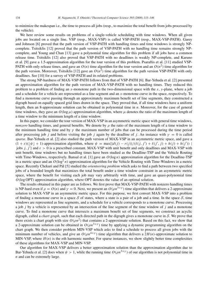
Fig. 1. Illustration of an instance of MAX-VSP-PATH constructed from an instance of 3-PARTITION.
3. NP-hardness of MAX-VSP-PATH
This section proves the NP-hardness of MAX-VSP-PATH.
Theorem 3.1. MAX-VSP-PATH is strongly NP-hard even if all jobs have unit benefit and ρ = O(n) holds.
Proof. We establish a polynomial reduction from a strong NP-hard problem, 3-PARTITION [7], whose instance isgiven by a set Z = {z1, z2, . . . , z3m} of 3m positive real numbers with zi ∈ (B/4, B/2), 1 ≤ i ≤ 3m, whereB = (1/m)
∑1≤i≤3m zi . The 3-PARTITION asks to determine whether the set Z can be partitioned into m disjoint
sets Z1, Z2, . . . , Zm , each of which satisfies∑
z∈Ziz = B and |Zi | = 3.
Given an instance I = (z1, z2, . . . , z3m) of 3-PARTITION, we construct an instance I ′ of MAX-VSP-PATH with3m jobs whose handling times correspond to z1, z2, . . . , z3m (and some other jobs) on a line in such a way thata vehicle can process exactly three jobs by a single traversal of the line in either direction to complete all jobsby m such traversals. More formally, I ′ is defined as follows. Let H, K ∈ R+ be positive real numbers. InstanceI ′
= (J1 ∪ J2, r, d, h, b, l, s) consists of two job sets J1 = { j1, j2, . . . , j3m} and J2 = { j ′1, j ′2, . . . , j ′m}. Each jobji ∈ J1 is at position p( ji ) = (i − 1)H ∈ R, has release time r( ji ) = 0, deadline d( ji ) = m(3m − 1)H + m B + mK ,and handling time h( ji ) = zi . On the other hand, each job j ′i ∈ J2 has handling time h( j ′i ) = K , and release time anddeadline r( j ′i ) = d( j ′i ) = i(3m − 1)H + i B + (i − 1)K . Jobs j ′1, j ′3, j ′5, . . . ∈ J2 with odd indices are at positionp( j3m) ∈ R and jobs j ′2, j ′4, j ′6, . . . ∈ J2 with even indices are at position p( j1) = 0. Let b( j) = 1, j ∈ J1 ∪ J2,p(s) = 0 and d(s) = +∞. Fig. 1 illustrates the time windows of jobs in instance I ′ in the position–time system. Weshow that a given instance I is a YES instance if and only if a single vehicle can process all jobs in J1 ∪ J2.
Suppose that I is a YES instance. Then Z can be partitioned into Zi = {zi,1, zi,2, zi,3}, i = 1, 2, . . . ,m with∑z∈Zi
z = B. Let J ′
i ⊆ J1 denote the set of three jobs that correspond to the three integers in Zi . We easily seethat the vehicle starting from position 0 at time 0 can process all jobs by m traversals of the line; The i th traversalprocesses the three jobs in J ′
i and job j ′i , taking (3m − 1)H travel time and B + K processing time. An example ofthe first traversal is indicated by dotted arrows in Fig. 1. Note that the release time and deadline of job j ′i are set to ber( j ′i ) = d( j ′i ) = i(3m − 1)H + i B + (i − 1)K , which is the arrival time at job j ′i of this schedule. Therefore, theinstance I ′ of MAX-VSP-PATH is a YES instance.
Conversely, suppose that a single vehicle can process all jobs in J1 ∪ J2. We see that the vehicle must process jobsin J2 in the order j ′1, j ′2, . . . , j ′m . Hence, the vehicle must traverse the line exactly m times. Job j ′m can be processedafter r( j ′m) = m(3m−1)H +m B+(m−1)K and its processing time finishes at time m(3m−1)H +m B+mK , where
H. Nagamochi, T. Ohnishi / Theoretical Computer Science 393 (2008) 133–146 137
the deadlines of all jobs in J1 are m(3m − 1)H + m B + mK . Hence, the vehicle must process all jobs in J1 before thevehicle processes the last job j ′m . From this, the vehicle must process 3m jobs in J1 while moving between position 0and p( j3m) m times. There is at most r( j ′i )− (r( j ′i−1)+ h( j ′i−1)) = (3m − 1)H + B time after finishing process ofjob j ′i−1 and before starting process of job j ′i (at release time r( j ′i )). Since it takes p( j3m) = (3m − 1)H time to travelthe line in one way, the vehicle can use B time for processing jobs in J1. On the other hand, B/4 < h( j) < B/2 holdsfor all j ∈ J1. Hence, the vehicle processes exactly three jobs in J1 in each traversal of the line. Therefore, instance Iof 3-PARTITION is a YES instance.
By choosing H = B/m and K = B, we see that ρ of I ′ is at most max{d( j) | j ∈ J1 ∪ J2}/min{h( j) | j ∈
J1 ∪ J2} = O(m) = O(|J1 ∪ J2|) since zi ∈ (B/4, B/2). �
Theorem 3.2. MAX-VSP-PATH is weakly NP-hard even if γ = 0 and ρ = O(n) hold.
Proof. We establish a polynomial reduction from an NP-hard problem, KNAPSACK [7], whose instance consists ofa set N of m items, 2m + 2 positive reals z1, z2, . . . , zm , v1, v2, . . . , vm , B and K , where zi and vi represent the sizeand value of item i ∈ N . The problem is to determine whether there exists a subset N ′
⊆ N such that∑i∈N ′
zi ≤ B and∑i∈N ′
vi ≥ K ,
where we can assume B ≤∑
i∈N zi and K ≤∑
i∈N vi without loss of generality.We first consider CONSTRAINED-KNAPSACK, an NP-hard problem defined from an instance I =
(z1, . . . , zm, v1, . . . , vm, B, K ) of KNAPSACK as follows. An instance I of CONSTRAINED-KNAPSACK consistsof m subinstances Ik = (z1, . . . , zm, v1, . . . , vm, B, K ) (k = 1, 2, . . . ,m) such that zi := zi + z∗, vi := vi + v∗
(i ∈ N ), B := B + kz∗, and K := K + kv∗ for z∗= 2
∑i∈N zi (>B) and v∗
= 2∑
i∈N vi (>K ), where for anyj ∈ N , it holds that B/z j = (B + 2k
∑i∈N zi )/(z j + 2
∑i∈N zi ) ≤ ((2k + 1)
∑i∈N zi )/(2
∑i∈N zi ) < k + 1. We
define instance I to be a YES instance if and only if one of the m subinstances I1, . . . , Im is a YES instance in thesense that some subinstance Ik admits a subset N ′
⊆ N that satisfies∑i∈N ′
zi ≤ B and∑i∈N ′
vi ≥ K for B and K defined for the k.
We claim that CONSTRAINED-KNAPSACK is also NP-hard by showing that I is a YES instance if and only if I isa YES instance. If I is a YES instance, then it holds that
∑i∈N ′ zi + |N ′
|z∗≤ B + |N ′
|z∗ and∑
i∈N ′ vi + |N ′|v∗
≥
K +|N ′|v∗, which implies that Ik for k = |N ′
| is a YES instance, i.e., I is a YES instance. Now we show the converse.If some subinstance Ik admits a subset N ′
⊆ N with∑
i∈N ′ zi ≤ B and∑
i∈N ′ vi ≥ K , then |N ′| = k holds because
otherwise it would hold that∑
i∈N ′ zi =∑
i∈N ′ zi + |N ′|z∗
≥ (k + 1)z∗ > B + kz∗= B (if |N ′
| ≥ k + 1), or∑i∈N ′ vi =
∑i∈N ′ vi + |N ′
|v∗≤ (1/2)v∗
+ (k − 1)v∗ < kv∗ < K + kv∗= K (if |N ′
| ≤ k − 1). Hence, ifI is a YES instance (i.e., some subinstance Ik is a YES instance), then I is also a YES instance. This proves thatCONSTRAINED-KNAPSACK is NP-hard.
To show the NP-hardness of MAX-VSP-PATH, it suffices to construct an instance I ′ for each subinstance Ik of aninstance I of CONSTRAINED-KNAPSACK (defined for an instance I of KNAPSACK) so that I ′ is a YES instanceif and only if Ik is a YES instance.
Given a subinstance Ik = (z1, . . . , zm, v1, . . . , vm, B, K ), we place the m items in N as jobs on a line, andlet a vehicle traverse the line from one end of the line to the other end only once before returning to the startpoint s so that any set of jobs processed by the single traversal of the line corresponds to a set N ′ of items thatsatisfies
∑i∈N ′ zi ≤ B. Formally instance I ′ is constructed as follows. Choose positive numbers H and M satisfying
H > B and M >∑
1≤i≤m vi . Instance I ′= (J1 ∪ { jm+1}, r, d, h, b, p, s) contains a start position s and m + 1
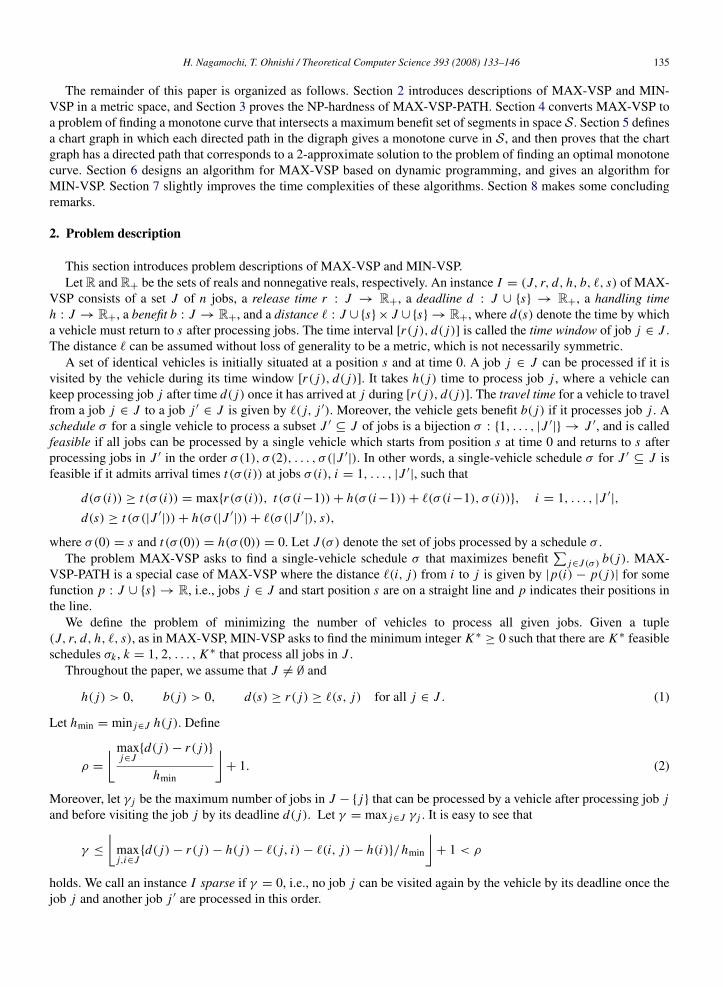
jobs, where J1 = { j1, j2, . . . , jm} consists of m jobs such that each job ji is at position p( ji ) = i H , has handlingtime h( ji ) = zi , benefit b( ji ) = vi , release time r( ji ) = p( ji ) = i H and deadline d( ji ) = r( ji ) + B = i H + B.The last job jm+1 is at position p( jm+1) = (m + 1)H , has handling time H , benefit b( jm) = M , release timer( jm+1) = (m + 1)H and deadline d( jm+1) = r( jm+1) + B. Let p(s) = 0 and d(s) = +∞. Fig. 2 shows the timewindows of jobs in I ′ in the position–time system. Note that by the assumption on the converted instance we haveρ = max{d( j)− r( j) | j ∈ J1 ∪ { jm+1}}/min{h( j) | j ∈ J1 ∪ { jm+1}} = B/min{zi | i ∈ N } < k + 1 = O(|J1|).Since H > B, once a vehicle processes job ji ∈ J1, it cannot visit any job ji ′ with i ′ < i before deadline d( ji ′).
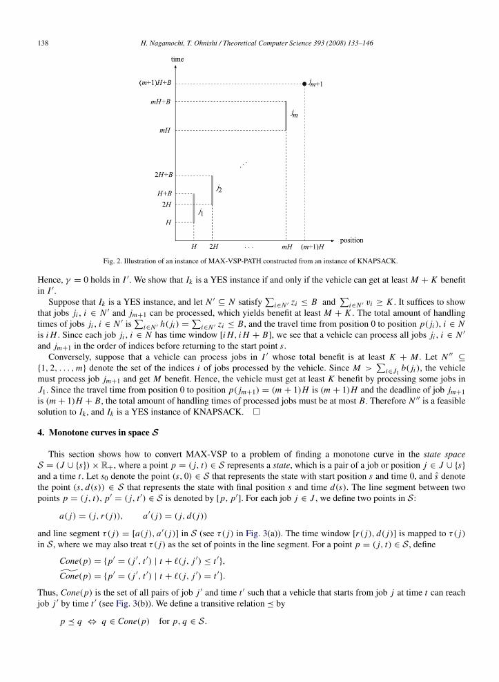
138 H. Nagamochi, T. Ohnishi / Theoretical Computer Science 393 (2008) 133–146
Fig. 2. Illustration of an instance of MAX-VSP-PATH constructed from an instance of KNAPSACK.
Hence, γ = 0 holds in I ′. We show that Ik is a YES instance if and only if the vehicle can get at least M + K benefitin I ′.
Suppose that Ik is a YES instance, and let N ′⊆ N satisfy
∑i∈N ′ zi ≤ B and
∑i∈N ′ vi ≥ K . It suffices to show
that jobs ji , i ∈ N ′ and jm+1 can be processed, which yields benefit at least M + K . The total amount of handlingtimes of jobs ji , i ∈ N ′ is
∑i∈N ′ h( ji ) =
∑i∈N ′ zi ≤ B, and the travel time from position 0 to position p( ji ), i ∈ N
is i H . Since each job ji , i ∈ N has time window [i H, i H + B], we see that a vehicle can process all jobs ji , i ∈ N ′
and jm+1 in the order of indices before returning to the start point s.Conversely, suppose that a vehicle can process jobs in I ′ whose total benefit is at least K + M . Let N ′′
⊆
{1, 2, . . . ,m} denote the set of the indices i of jobs processed by the vehicle. Since M >∑
i∈J1b( ji ), the vehicle
must process job jm+1 and get M benefit. Hence, the vehicle must get at least K benefit by processing some jobs inJ1. Since the travel time from position 0 to position p( jm+1) = (m + 1)H is (m + 1)H and the deadline of job jm+1is (m + 1)H + B, the total amount of handling times of processed jobs must be at most B. Therefore N ′′ is a feasiblesolution to Ik , and Ik is a YES instance of KNAPSACK. �
4. Monotone curves in space S
This section shows how to convert MAX-VSP to a problem of finding a monotone curve in the state spaceS = (J ∪ {s})× R+, where a point p = ( j, t) ∈ S represents a state, which is a pair of a job or position j ∈ J ∪ {s}and a time t . Let s0 denote the point (s, 0) ∈ S that represents the state with start position s and time 0, and s denotethe point (s, d(s)) ∈ S that represents the state with final position s and time d(s). The line segment between twopoints p = ( j, t), p′
= ( j, t ′) ∈ S is denoted by [p, p′]. For each job j ∈ J , we define two points in S:
a( j) = ( j, r( j)), a′( j) = ( j, d( j))
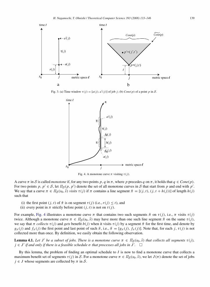
and line segment τ( j) = [a( j), a′( j)] in S (see τ( j) in Fig. 3(a)). The time window [r( j), d( j)] is mapped to τ( j)in S, where we may also treat τ( j) as the set of points in the line segment. For a point p = ( j, t) ∈ S, define
Cone(p) = {p′= ( j ′, t ′) | t + `( j, j ′) ≤ t ′},
Cone(p) = {p′= ( j ′, t ′) | t + `( j, j ′) = t ′}.
Thus, Cone(p) is the set of all pairs of job j ′ and time t ′ such that a vehicle that starts from job j at time t can reachjob j ′ by time t ′ (see Fig. 3(b)). We define a transitive relation � by
p � q ⇔ q ∈ Cone(p) for p, q ∈ S.
H. Nagamochi, T. Ohnishi / Theoretical Computer Science 393 (2008) 133–146 139
Fig. 3. (a) Time window τ( j) = [a( j), a′( j)] of job j ; (b) Cone(p) of a point p in S.
Fig. 4. A monotone curve π visiting τ( j).
A curve π in S is called monotone if, for any two points p, q in π , where p precedes q on π , it holds that q ∈ Cone(p).For two points p, p′
∈ S, let ΠS(p, p′) denote the set of all monotone curves in S that start from p and end with p′.We say that a curve π ∈ ΠS(s0, s) visits τ( j) if π contains a line segment π = [( j, t), ( j, t + h( j))] of length h( j)such that
(i) the first point ( j, t) of π is on segment τ( j) (i.e., r( j) ≤ t), and(ii) every point in π strictly before point ( j, t) is not on τ( j).
For example, Fig. 4 illustrates a monotone curve π that contains two such segments π on τ( j), i.e., π visits τ( j)twice. Although a monotone curve π ∈ ΠS(s0, s) may have more than one such line segment π on the same τ( j),we say that π collects τ( j) and gets benefit b( j) when it visits τ( j) by a segment π for the first time, and denote bygπ ( j) and fπ ( j) the first point and last point of such π , i.e., π = [gπ ( j), fπ ( j)]. Note that, for each j , τ( j) is notcollected more than once. By definition, we easily obtain the following observation.
Lemma 4.1. Let J ′ be a subset of jobs. There is a monotone curve π ∈ ΠS(s0, s) that collects all segments τ( j),j ∈ J ′ if and only if there is a feasible schedule σ that processes all jobs in J ′. �
By this lemma, the problem of finding an optimal schedule to I is now to find a monotone curve that collects amaximum benefit set of segments τ( j) in S. For a monotone curve π ∈ ΠS(s0, s), we let J (π) denote the set of jobsj ∈ J whose segments are collected by π in S.
140 H. Nagamochi, T. Ohnishi / Theoretical Computer Science 393 (2008) 133–146
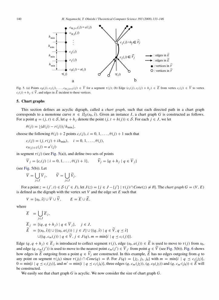
Fig. 5. (a) Points c0( j), c1( j), . . . , cθ( j)+1( j) ∈ V for a segment τ( j); (b) Edge (ci ( j), ci ( j) + h j ) ∈ E from vertex ci ( j) ∈ V to vertexci ( j)+ h j ∈ V , and edges in E incident to these vertices.
5. Chart graphs
This section defines an acyclic digraph, called a chart graph, such that each directed path in a chart graphcorresponds to a monotone curve π ∈ ΠS(s0, s). Given an instance I , a chart graph G is constructed as follows.For a point q = ( j, t) ∈ S, let q + h j denote the point ( j, t + h( j)) ∈ S. For each j ∈ J , we let
θ( j) = b(d( j)− r( j))/hminc,
choose the following θ( j)+ 2 points ci ( j), i = 0, 1, . . . , θ( j)+ 1 such that
ci ( j) = ( j, r( j)+ ihmin), i = 0, 1, . . . , θ( j),
cθ( j)+1( j) = a′( j)
in segment τ( j) (see Fig. 5(a)), and define two sets of points
V j = {ci ( j) | i = 0, 1, . . . , θ( j)+ 1}, V j = {q + h j | q ∈ V j }
(see Fig. 5(b)). Let
V =
⋃j∈J
V j , V =
⋃j∈J
V j .
For a point z = ( j ′, t) ∈ S ( j ′ ∈ J ), let J (z) = { j ∈ J −{ j ′} | τ( j)∩Cone(z) 6= ∅}. The chart graph G = (V, E)is defined as the digraph with the vertex set V and the edge set E such that
V = {s0, s} ∪ V ∪ V , E = E ∪ E,
where
E =
⋃j∈J
E j ,
E j = {(q, q + h j ) | q ∈ V j }, j ∈ J,
E = {(s0, s)} ∪ {(s0, a( j)) | j ∈ J } ∪ {(q, s) | q ∈ V , q � s}
∪{(q, cm( j)) | q ∈ V , j ∈ J (q),m = min{i | q � ci ( j)}}.
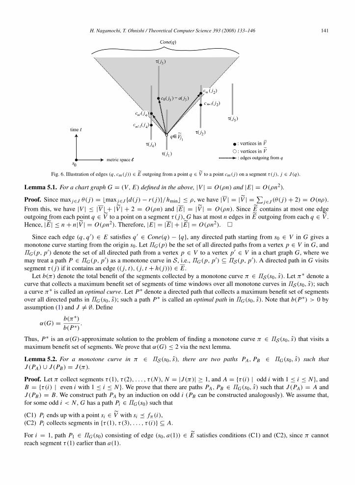
Edge (q, q + h j ) ∈ E j is introduced to collect segment τ( j), edge (s0, a( j)) ∈ E is used to move to τ( j) from s0,and edge (q, cm( j ′)) is used to move to the nearest point cm( j ′) ∈ V j ′ from point q ∈ V (see Fig. 5(b)). Fig. 6 showshow edges in E outgoing from a point q ∈ V j are constructed. In this example, E has no edges outgoing from q toany point on segment τ( j5) since τ( j5) ∩ Cone(q) = ∅. For J (q) = { j2, j3, j4} with m = min{i | q � ci ( j2)},0 = min{i | q � ci ( j3)}, and m′
= min{i | q � ci ( j4)}, three edges (q, cm( j2)), (q, c0( j3)) and (q, cm′( j4)) ∈ E willbe constructed.
We easily see that chart graph G is acyclic. We now consider the size of chart graph G.
H. Nagamochi, T. Ohnishi / Theoretical Computer Science 393 (2008) 133–146 141
Fig. 6. Illustration of edges (q, cm ( j)) ∈ E outgoing from a point q ∈ V to a point cm ( j) on a segment τ( j), j ∈ J (q).
Lemma 5.1. For a chart graph G = (V, E) defined in the above, |V | = O(ρn) and |E | = O(ρn2).
Proof. Since max j∈J θ( j) = bmax j∈J {d( j) − r( j)}/hminc ≤ ρ, we have |V | = |V | =∑
j∈J (θ( j) + 2) = O(nρ).
From this, we have |V | ≤ |V | + |V | + 2 = O(ρn) and |E | = |V | = O(ρn). Since E contains at most one edgeoutgoing from each point q ∈ V to a point on a segment τ( j), G has at most n edges in E outgoing from each q ∈ V .Hence, |E | ≤ n + n|V | = O(ρn2). Therefore, |E | = |E | + |E | = O(ρn2). �
Since each edge (q, q ′) ∈ E satisfies q ′∈ Cone(q) − {q}, any directed path starting from s0 ∈ V in G gives a
monotone curve starting from the origin s0. Let ΠG(p) be the set of all directed paths from a vertex p ∈ V in G, andΠG(p, p′) denote the set of all directed path from a vertex p ∈ V to a vertex p′
∈ V in a chart graph G, where wemay treat a path P ∈ ΠG(p, p′) as a monotone curve in S, i.e., ΠG(p, p′) ⊆ ΠS(p, p′). A directed path in G visitssegment τ( j) if it contains an edge (( j, t), ( j, t + h( j))) ∈ E .
Let b(π) denote the total benefit of the segments collected by a monotone curve π ∈ ΠS(s0, s). Let π∗ denote acurve that collects a maximum benefit set of segments of time windows over all monotone curves in ΠS(s0, s); sucha curve π∗ is called an optimal curve. Let P∗ denote a directed path that collects a maximum benefit set of segmentsover all directed paths in ΠG(s0, s); such a path P∗ is called an optimal path in ΠG(s0, s). Note that b(P∗) > 0 byassumption (1) and J 6= ∅. Define
α(G) =b(π∗)
b(P∗).
Thus, P∗ is an α(G)-approximate solution to the problem of finding a monotone curve π ∈ ΠS(s0, s) that visits amaximum benefit set of segments. We prove that α(G) ≤ 2 via the next lemma.
Lemma 5.2. For a monotone curve in π ∈ ΠS(s0, s), there are two paths PA, PB ∈ ΠG(s0, s) such thatJ (PA) ∪ J (PB) = J (π).
Proof. Let π collect segments τ(1), τ(2), . . . , τ (N ), N = |J (π)| ≥ 1, and A = {τ(i) | odd i with 1 ≤ i ≤ N }, andB = {τ(i) | even i with 1 ≤ i ≤ N }. We prove that there are paths PA, PB ∈ ΠG(s0, s) such that J (PA) = A andJ (PB) = B. We construct path PA by an induction on odd i (PB can be constructed analogously). We assume that,for some odd i < N , G has a path Pi ∈ ΠG(s0) such that
(C1) Pi ends up with a point si ∈ V with si � fπ (i),(C2) Pi collects segments in {τ(1), τ (3), . . . , τ (i)} ⊆ A.
For i = 1, path P1 ∈ ΠG(s0) consisting of edge (s0, a(1)) ∈ E satisfies conditions (C1) and (C2), since π cannotreach segment τ(1) earlier than a(1).
142 H. Nagamochi, T. Ohnishi / Theoretical Computer Science 393 (2008) 133–146
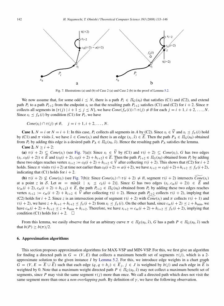
Fig. 7. Illustrations (a) and (b) of Case 2 (a) and Case 2 (b) in the proof of Lemma 5.2.
We now assume that, for some odd i ≤ N , there is a path Pi ∈ ΠG(s0) that satisfies (C1) and (C2), and extendpath Pi to a path Pi+2 from the endpoint si so that the resulting path Pi+2 satisfies (C1) and (C2) for i + 2. Since πcollects all segments in {τ( j) | i + 1 ≤ j ≤ N }, we have Cone( fπ (i)) ∩ τ( j) 6= ∅ for each j = i + 1, i + 2, . . . , N .Since si � fπ (i) by condition (C1) for Pi , we have
Cone(si ) ∩ τ( j) 6= ∅, j = i + 1, i + 2, . . . , N .
Case 1. N = i or N = i + 1: In this case, Pi collects all segments in A by (C2). Since si ∈ V and si � fπ (i) holdby (C1) and π visits s, we have s ∈ Cone(si ) and there is an edge (si , s) ∈ E . Then the path PA ∈ ΠG(s0) obtainedfrom Pi by adding this edge is a desired path PA ∈ ΠG(s0, s). Hence the resulting path PA satisfies the lemma.
Case 2. N ≥ i + 2:(a) τ(i + 2) ⊆ Cone(si ) (see Fig. 7(a)): Since si ∈ V by (C1) and τ(i + 2) ⊆ Cone(si ), G has two edges
(si , c0(i + 2)) ∈ E and (c0(i + 2), c0(i + 2)+ hi+2) ∈ E . Then the path Pi+2 ∈ ΠG(s0) obtained from Pi by addingthese two edges reaches vertex si+2 := c0(i + 2)+ hi+2 ∈ V after collecting τ(i + 2). This shows that (C2) for i + 2holds. Since π visits τ(i +2) at time not earlier than c0(i +2) = a(i +2), we have si+2 = c0(i +2)+hi+2 � fπ (i +2),indicating that (C1) holds for i + 2.
(b) τ(i + 2) 6⊆ Cone(si ) (see Fig. 7(b)): Since Cone(si ) ∩ τ(i + 2) 6= ∅, segment τ(i + 2) intersects Cone(si )
at a point z in S. Let m = min{k | si � ck(i + 2)}. Since G has two edges (si , cm(i + 2)) ∈ E and(cm(i + 2), cm(i + 2) + hi+2) ∈ E , the path Pi+2 ∈ ΠG(s0) obtained from Pi by adding these two edges reachesvertex si+2 := cm(i + 2) + hi+2 ∈ V after collecting τ(i + 2). Hence path Pi+2 collects τ(i + 2), implying that(C2) holds for i + 2. Since z is an intersection point of segment τ(i + 2) with Cone(si ) and π collects τ(i + 1) andτ(i + 2), we have z + hi+1 + hi+2 � fπ (i + 2) from si � fπ (i). On the other hand, since cm(i + 2) � z + hmin, wehave cm(i + 2)+ hi+2 � z + hmin + hi+2. Therefore, we have si+2 = cm(i + 2)+ hi+2 � fπ (i + 2), implying thatcondition (C1) holds for i + 2. �
From this lemma, we easily observe that for an arbitrary curve π ∈ ΠS(s0, s), G has a path P ∈ ΠG(s0, s) suchthat b(P) ≥ b(π)/2.
6. Approximation algorithms
This section proposes approximation algorithms for MAX-VSP and MIN-VSP. For this, we first give an algorithmfor finding a directed path in G = (V, E) that collects a maximum benefit set of segments τ( j), which is a 2-approximate solution to the given instance I by Lemma 5.2. For this, we introduce edge weights in a chart graphG = (V, E = E ∪ E) such that each edge (q, q + h j ) ∈ E j , j ∈ J is weighted by b( j) and each edge in E isweighted by 0. Note that a maximum weight directed path P ∈ ΠG(s0, s) may not collect a maximum benefit set ofsegments, since P may visit the same segment τ( j) more than once. We call a directed path which does not visit thesame segment more than once a non-overlapping path. By definition of γ , we have the following observation.
H. Nagamochi, T. Ohnishi / Theoretical Computer Science 393 (2008) 133–146 143
Lemma 6.1. Let P ∈ ΠG(s0) be a path, and e1, e2, . . . , eK be the edges in E contained in P, where P passes throughthese edges in this order, and each edge ei is on segment τ( ji ), i.e., ei ∈ E ji . If jk 6∈ { jk−1, jk−2, . . . , jmax{1,k−γ−1}}
holds for all k with 1 < k ≤ K , then P is a non-overlapping path. �
We use dynamic programming to compute a maximum benefit non-overlapping path in G. To avoid includingoverlapping paths during computation of the dynamic programming algorithm, paths in ΠG(s0, v) for each vertexv ∈ V will be distinguished by the last γ + 1 segments collected by the paths.
Theorem 6.2. For an instance I to MAX-VSP, a 2-approximate solution can be obtained in O(ρn3+γ ) time.
Proof. Let G = (V, E) be a chart graph obtained from I . To compute a maximum weight non-overlapping pathP ∈ ΠG(s0, s), we design a dynamic programming algorithm as follows. Let Jm denote the family of all sequences ofat most m distinct jobs in J = {1, 2, . . . , n}. For a sequence µ ∈ Jm , let |µ| denote the number of jobs in µ, and µ(i)denote the i th job in µ. We denote by µ−µ(1) the sequence obtained by removing µ(1) from µ, and by µ′
= µ⊕ jthe sequence obtained by adding job j to µ as the last job of µ′. For a vertex v ∈ V and a sequence µ ∈ Jγ+1,W [v, µ] ∈ R+ is defined as follows.
(i) If |µ| = γ + 1, then let W [v, µ] be the maximum weight of a non-overlapping path P ∈ ΠG(s0, v) thatcollects segments τ(µ(γ +1)), τ (µ(γ )), . . . , τ (µ(1)) in this order, where P may collect some other segmentsbefore collecting τ(µ(γ + 1)), but it collects no segment other than τ(µ(γ )), . . . , τ (µ(1)) after collectingτ(µ(γ + 1)).
(ii) If |µ| ≤ γ , then let W [v, µ] be the maximum weight of a non-overlapping path P ∈ ΠG(s0, v) that collectssegments τ(µ(|µ|)), τ (µ(|µ| − 1)), . . . , τ (µ(1)) in this order, where P collects no other segments thanτ(µ(i)), i = 1, 2, . . . , |µ|.
By definition of W , a recursion formula of W [v, µ] with v ∈ V and µ ∈ Jγ+1 is given as follows. LetV −(v) = {u | (u, v) ∈ E} for each v ∈ V .
Case 1. There is no u ∈ V −(v) satisfying (u, v) ∈ E : Then we have
W [v, µ] = max{W [u, µ] | u ∈ V −(v)}. (3)
Case 2. There is u ∈ V −(v) satisfying (u, v) ∈ E (where such u is unique): Let u∗ denote such u, and j∗ denotethe job such that u∗
∈ V j∗ . Then we have
W [v, µ] =
−∞ if j∗ ∈ {µ(i) | 2 ≤ i ≤ |µ|}
W1 if j∗ 6∈ {µ(i) | 1 ≤ i ≤ |µ|}
W2 if j∗ = µ(1) and |µ| ≤ γ
max{W2,W3} if j∗ = µ(1) and |µ| = γ + 1,
where
W1 = max{W [u, µ] | u ∈ V −(v)− {u∗}}, (4)
W2 = W [u∗, µ−µ(1)] + b( j∗), (5)
W3 = max{W [u∗, (µ−µ(1))⊕ j] + b( j∗) | j ∈ J −{µ(i) | 1 ≤ i ≤ |µ|}} (6)
(W1 = −∞ if V −(v)− {u∗} = ∅).
The boundary condition of the recursive formula is given by
W [s0, µ] =
{0 if |µ| = 0−∞ otherwise.
(7)
Based on the above formula, we can compute {W [s, µ] | µ ∈ Jγ+1} by dynamic programming considering verticesin a topological order of G. By Lemma 6.1, we can find a maximum weight non-overlapping path by choosingthe maximum W ∗
γ+1 = max{W [s, µ] | µ ∈ Jγ+1}. The number of sequences in Jγ+1 is O(n1+γ ). Since G has
O(ρn2) edges in E , it takes O(ρn3+γ ) time to compute all W [v, µ] in (3) and all W1 in (4). For each W [v, µ],we can compute W2 in (5) in O(1) time and W3 in (6) in O(n) time. Since G has at most O(ρn) edges in E ,it takes O(ρn3+γ ) time to compute all W2 and W3. We can also detect a path Pγ+1 ∈ ΠG(s0, s) that attains
144 H. Nagamochi, T. Ohnishi / Theoretical Computer Science 393 (2008) 133–146
the maximum weight W ∗
γ+1 in O(ρn3+γ ) time (note that such a path exists since the set of edges incident to s is
{(s0, s)} ∪ {(q, s) | q ∈ V , q � s} ⊆ E in G).Finally we show that path Pγ+1 ∈ ΠG(s0, s) can be obtained in the same time complexity even if γ is not
available in advance. For each m = 1, 2, . . . , we let the above algorithm compute the maximum weight W ∗
m+1and a corresponding path Pm+1 ∈ ΠG(s0, s) by setting γ := m until a non-overlapping path Pm+1 is obtained. Notethat in general a path in ΠG(s0, s) may not be non-overlapping if m < γ . However, a non-overlapping path Pm+1will be found for some m ≤ γ , and any such path attains the maximum weight among all non-overlapping paths inΠG(s0, s). The total time complexity is O(
∑1≤m≤γ ρn3+m) = O(ρn3+γ ). �
Based on this theorem, we design an O(ρn4+γ ) time algorithm that delivers a 2H(n)-approximate solution toMIN-VSP, where H(n) is the nth harmonic number. For this, we here review a result on the set cover problem. Givena finite set X and a family F = {Si | i = 1, 2, . . . , q} of subsets of X such that X ⊆ ∪1≤i≤q Si , the problem asksto find a smallest subset F∗
⊆ F such that X ⊆ ∪S∈F∗ S. The problem is known to be NP-hard [7]. Starting withF ′
:= ∅, a simple greedy algorithm repeats finding a subset S ∈ F − F ′ that maximizes |S ∩ (X − ∪S′∈F ′ S′)|
and updating F ′:= F ′
∪ {S} until X − ∪S′∈F ′ S′= ∅ holds. It is known that the resulting subset F ′
⊆ F is anH(|X |)-approximate solution, i.e., |F ′
| ≤ H(|X |)|F∗| holds for an optimal solution F∗ [8].
Theorem 6.3. For an instance I of MIN-VSP, a 2H(n)-approximate solution can be obtained in O(ρn4+γ ) time.
Proof. Let K ∗ be the minimum number of vehicles that can process all jobs in I . Define benefit b by b( j) = 1,j ∈ J , consider the chart graph G for the instance I with b. By Lemma 5.2, we see that there exists a set of at most2K ∗ paths of G such that any segment τ( j), j ∈ J , is collected by one path of the set. We now consider the problemof finding a smallest set P of paths in ΠG(s0, s) such that, for each j ∈ J , at least one edge in E j is contained in oneof the paths in P . We can regard the problem as the set cover problem with X = J and F = {J (P) | P ∈ ΠG(s0, s)}.The greedy algorithm in this case can be implemented as follows. For a subset F ′, where J ′
= ∪S′∈F ′ S′, we see thatP ∈ ΠG(s0, s) that maximizes |J (P)∩(J − J ′)| can be obtained by computing a path P ∈ ΠG ′(s0, s) that collects themaximum number of jobs in the chart graph G ′ constructed from the set J − J ′ of remaining jobs. As observed in theproof of Theorem 6.2, such a path P ∈ ΠG ′(s0, s) can be computed in O(ρn3+γ ) time. Hence the greedy algorithmruns in O(|X |ρn3+γ ) = O(ρn4+γ ) time and delivers an H(|X |)-approximate solution, i.e., a set of 2K ∗ H(n) pathsin ΠG(s0, s) that covers all E j , j ∈ J , which is a 2H(n)-approximate solution to MIN-VSP. �
7. Algorithms for sparse instances
In this section, we consider sparse instances I of MAX-VSP and MIN-VSP, and improve the time complexities ofthe algorithms in the previous section.
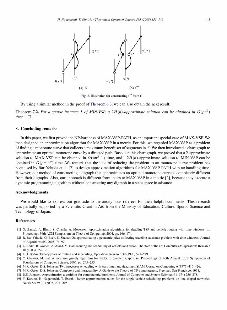
Since γ = 0 in a sparse instance I , the same segment τ( j) is not visited by any path P ∈ ΠG(s0, s) after τ( j) andsome other segment τ( j ′) are collected. However, in the chart graph G, there may exist a segment τ( j) in which sometwo vertices ci ( j)+ h j and ci ′ are the same point in the space S, i.e., ci ( j)+ h j = ci ′ ∈ V j ∩ V j (see Fig. 8(a)) andtwo edges (ci ( j), ci ( j) + h j ), (ci ( j) + h j = ci ′ , ci ′ + h j ) ∈ E can be traversed by a path P ∈ ΠG(s0, s). To avoidconstructing paths that traverse two such consecutive edges in E , we modify chart graph G = (V, E = E ∪ E) asfollows. We split each vertex v ∈ V ∩ V into two new vertices v+ and v− by replacing each directed edge (u, v) ∈ E(resp., (v, u) ∈ E) with (u, v+) (resp., (v−, u)) and each directed edge (u, v) ∈ E (resp., (v, u) ∈ E) with (u, v−)
(resp., (v+, u)), as shown in Fig. 8(b). Let G ′= (V ′, E ′) be the graph obtained from G by applying the above
procedure for all vertices v ∈ V ∩ V . Note that |V ′| ≤ 2|V | = O(ρn) and |E ′
| = |E | = O(ρn2) hold. We easily seethat
α(G ′) = α(G) ≤ 2
and that every path in ΠG ′(s0, s) is a non-overlapping path. Hence, by computing a maximum weight path P in G ′,we can obtain a 2-approximate solution to a sparse instance I . This can be done in O(|V ′
| + |E ′|) time. Therefore
we establish the following theorem.
Theorem 7.1. For a sparse instance I of MAX-VSP, a 2-approximate solution can be obtained in O(ρn2) time. �
H. Nagamochi, T. Ohnishi / Theoretical Computer Science 393 (2008) 133–146 145
Fig. 8. Illustration for constructing G′ from G.
By using a similar method in the proof of Theorem 6.3, we can also obtain the next result.
Theorem 7.2. For a sparse instance I of MIN-VSP, a 2H(n)-approximate solution can be obtained in O(ρn3)
time. �
8. Concluding remarks
In this paper, we first proved the NP-hardness of MAX-VSP-PATH, as an important special case of MAX-VSP. Wethen designed an approximation algorithm for MAX-VSP in a metric. For this, we regarded MAX-VSP as a problemof finding a monotone curve that collects a maximum benefit set of segments in S. We then introduced a chart graph toapproximate an optimal monotone curve by a directed path. Based on this chart graph, we proved that a 2-approximatesolution to MAX-VSP can be obtained in O(ρn3+γ ) time, and a 2H(n)-approximate solution to MIN-VSP can beobtained in O(ρn4+γ ) time. We remark that the idea of reducing the problem to an monotone curve problem hasbeen used by Bar-Yehuda et al. [2] to design approximation algorithms for MAX-VSP-PATH with no handling time.However, our method of constructing a digraph that approximates an optimal monotone curve is completely differentfrom their digraphs. Also, our approach is different from theirs to MAX-VSP in a metric [2], because they execute adynamic programming algorithm without constructing any digraph in a state space in advance.
Acknowledgments
We would like to express our gratitude to the anonymous referees for their helpful comments. This researchwas partially supported by a Scientific Grant in Aid from the Ministry of Education, Culture, Sports, Science andTechnology of Japan.
References
[1] N. Bansal, A. Blum, S. Chawla, A. Meyerson, Approximation algorithms for deadline-TSP and vehicle routing with time-windows, in:Proceedings 36th ACM Symposium on Theory of Computing, 2004, pp. 166–174.
[2] R. Bar-Yehuda, G. Even, S. Shahar, On approximating a geometric prize-collecting traveling salesman problem with time windows, Journalof Algorithms 55 (2005) 76–92.
[3] L. Bodin, B. Golden, A. Assad, M. Ball, Routing and scheduling of vehicles and crews: The state of the art, Computers & Operations Research10 (1983) 62–212.
[4] L.D. Bodin, Twenty years of routing and scheduling, Operations Research 39 (1990) 571–579.[5] C. Chekuri, M. Pal, A recursive greedy algorithm for walks in directed graphs, in: Proceedings of 46th Annual IEEE Symposium of
Foundations of Computer Science, 2005, pp. 245–253.[6] M.R. Garey, D.S. Johnson, Two-processor scheduling with start times and deadlines, SIAM Journal on Computing 6 (1977) 416–426.[7] M.R. Garey, D.S. Johnson, Computers and Intractability, A Guide to the Theory of NP-completeness, Freeman, San Francisco, 1978.[8] D.S. Johnson, Approximation algorithms for combinatorial problems, Journal of Computer and System Sciences 9 (1974) 256–278.[9] Y. Karuno, H. Nagamochi, T. Ibaraki, Better approximation ratios for the single-vehicle scheduling problems on line-shaped networks,
Networks 39 (4) (2002) 203–209.
146 H. Nagamochi, T. Ohnishi / Theoretical Computer Science 393 (2008) 133–146
[10] Y. Karuno, H. Nagamochi, Scheduling vehicles on trees, Pacific Journal of Optimization 1 (2005) 527–543.[11] H. Psaraftis, M.M. Solomon, L. Magnanti, T .U. Kim, Routing and scheduling on a shoreline with release times, Management Science 36
(1990) 212–223.[12] J.N. Tsitsiklis, Special cases of traveling salesman and repairman problems with time windows, Networks 22 (1992) 263–282.[13] G. Young, C. Chan, Single-vehicle scheduling with time window constraints, Journal of Scheduling 2 (1999) 175–187.