Embed Size (px)
Citation preview

SIAM J. SCI. COMPUT. c© 2017 Society for Industrial and Applied MathematicsVol. 39, No. 4, pp. A1558–A1585
APPROXIMATING SPECTRAL SUMS OF LARGE-SCALEMATRICES USING STOCHASTIC CHEBYSHEV
APPROXIMATIONS∗
INSU HAN† , DMITRY MALIOUTOV‡ , HAIM AVRON§ , AND JINWOO SHIN¶
Abstract. Computation of the trace of a matrix function plays an important role in manyscientific computing applications, including applications in machine learning, computational physics(e.g., lattice quantum chromodynamics), network analysis, and computational biology (e.g., proteinfolding), just to name a few application areas. We propose a linear-time randomized algorithm forapproximating the trace of matrix functions of large symmetric matrices. Our algorithm is basedon coupling function approximation using Chebyshev interpolation with stochastic trace estimators(Hutchinson’s method), and as such requires only implicit access to the matrix, in the form ofa function that maps a vector to the product of the matrix and the vector. We provide rigorousapproximation error in terms of the extremal eigenvalue of the input matrix, and the Bernstein ellipsethat corresponds to the function at hand. Based on our general scheme, we provide algorithmswith provable guarantees for important matrix computations, including log-determinant, trace ofmatrix inverse, Estrada index, Schatten p-norm, and testing positive definiteness. We experimentallyevaluate our algorithm and demonstrate its effectiveness on matrices with tens of millions dimensions.
Key words. spectral function, matrix computation, Chebyshev approximation, Hutchinson’smethod
AMS subject classification. 68W25
DOI. 10.1137/16M1078148
1. Introduction. Given a symmetric matrix A ∈ Rd×d and function f : R→ R,we study how to efficiently compute
Σf (A) = tr(f(A)) =d∑i=1
f(λi),(1)
where λ1, . . . , λd are eigenvalues of A. We refer to such sums as spectral sums (alsoreferred to as trace functions). Spectral sums depend only on the eigenvalues of Aand so they are spectral functions, although not every spectral function is a spectralsum. Nevertheless, the class of spectral sums is rich and includes useful spectralfunctions. For example, if A is also positive definite then Σlog(A) = log det(A), i.e.the log-determinant of A.
∗Submitted to the journal’s Methods and Algorithms for Scientific Computing section June 1,2016; accepted for publication (in revised form) March 13, 2017; published electronically August 22,2017. This article is partially based on preliminary results published in the proceeding of the 32ndInternational Conference on Machine Learning (ICML 2015).
http://www.siam.org/journals/sisc/39-4/M107814.htmlFunding: The work of the third author was supported by the XDATA program of the Defense
Advanced Research Projects Agency (DARPA), administered through Air Force Research Laboratorycontract FA8750-12-C-0323.†School of Electrical Engineering, Korea Advanced Institute of Science and Technology, Dacjeon
Korea ([email protected]).‡Business Analytics and Mathematical Sciences, IBM Research, Yorktown Heights, NY, 10598
([email protected]).§Department of Applied Mathematics, Tel Aviv University/Tel Aviv 6997801, Israel
([email protected]).¶School of Electrical Engineering, Korea Advanced Institute of Science and Technology, Dacjeon
Korea ([email protected]).
A1558

APPROXIMATING SPECTURAL SUMS A1559
Indeed, there are many real-world applications in which spectral sums play animportant role. For example, the log-determinant appears ubiquitously in machinelearning applications including Gaussian graphical and Gaussian process models [38,36, 13], partition functions of discrete graphical models [29], minimum-volume ellip-soids [44], metric learning, and kernel learning [10]. The trace of the matrix inverse(Σf (A) for f(x) = 1/x) is frequently computed for the covariance matrix in uncer-tainty quantification [9, 27] and lattice quantum chromodynamics [39]. The Estradaindex (Σexp(A)) has been initially developed for topological index of protein folding inthe study of protein functions and protein-ligand interactions [15, 12], and currentlyit appears in numerous other applications, e.g., statistical thermodynamics [18, 17],information theory [7], and network theory [19, 16] ; see Gutman et al. [22] for moreapplications. The Schatten p-norm (Σf (A>A)1/p for f(x) = xp/2 for p ≥ 1 ) has beenapplied to recover low-rank matrix [34] and sparse MRI reconstruction [30].
The computation of the aforementioned spectral sums for large-scale matricesis a challenging task. For example, the standard method for computing the log-determinant uses the Cholesky decomposition (if A = LLT is a Cholesky decompo-sition, then log det(A) = 2
∑i logLii). In general, the computational complexity of
Cholesky decomposition is cubic with respect to the number of variables, i.e., O(d3).For large-scale applications involving more than tens of thousands of dimensions, thisis obviously not feasible. If the matrix is sparse, one might try to take advantage ofsparse decompositions. As long as the amount of fill-in during the factorizations isnot too big, a substantial improvement in running time can be expected. Neverthe-less, the worst case still requires Θ(d3). In particular, if the sparsity structure of A israndom-like, as is common in several of the aforementioned applications, then littleimprovement can be expected with sparse methods.
Our aim is to design an efficient algorithm that is able to compute accurateapproximations to spectral sums for matrices with tens of millions of variables.
1.1. Contributions. We propose a randomized algorithm for approximatingspectral sums based on a combination of stochastic trace-estimators and Chebyshevinterpolation. Our algorithm first computes the coefficients of a Chebyshev approxi-mation of f . This immediately leads to an approximation of the spectral sums as thetrace of power series of the input matrix. We then use a stochastic trace-estimator toestimate this trace. In particular, we use Hutchinson’s method [25].
One appealing aspect of Hutchinson’s method is that it does not require an explicitrepresentation of the input matrix; Hutchinson’s method requires only an implicit rep-resentation of the matrix as an operation that maps a vector to the product of thematrix with the vector. In fact, this property is inherited by our algorithm to itsentirety: our algorithm only needs access to an implicit representation of the matrixas an operation that maps a vector to the product of the matrix with the vector. Inaccordance, we measure the complexity of our algorithm in terms of the number ofmatrix-vector products that it requires. We establish rigorous bounds on the num-ber of matrix-vector products for attaining a ε-multiplicative approximation of thespectral sums based on ε, the failure probability, and the range of the function overits Bernstein ellipse (see Theorem 3.1 for details). In particular, Theorem 3.1 impliesthat if the range is Θ(1), then the algorithm provides ε-multiplicative approximationguarantee using a constant amount of matrix-vector products for any constant ε > 0and constant failure probability.
The overall time complexity of our algorithm is O(t·‖A‖mv), where t is the numberof matrix-vector products (as established by our analysis) and ‖A‖mv is the cost of

A1560 I. HAN, D. MALIOUTOV, H. AVRON, AND J. SHIN
multiplying A by a vector. One overall assumption is that matrix-vector productscan be computed efficiently, i.e., ‖A‖mv is small. For example, if A is sparse then‖A‖mv = O(nnz(A)), i.e., the number of non-zero entries in A. Other cases that admitfast matrix-vector products are low-rank matrices (which allow fast multiplicationby factorization), or Fourier (or Hadamard, Walsh, Toeplitz) matrices using the fastFourier transform. The proposed algorithm is also very easy to parallelize.
We then proceed to discuss applications of the proposed algorithm. We give rig-orous bounds for using our algorithm for approximating the log-determinant, trace ofthe inverse of a matrix, the Estrada index, and the Schatten p-norm. These correspondto continuous functions f(x) = log x, f(x) = 1/x, f(x) = exp(x), and f(x) = xp/2,respectively. We also use our algorithm to construct a novel algorithm for testing pos-itive definiteness in the property testing framework. Our algorithm, which is basedon approximating the spectral sums for 1−sign(x), is able to test positive definitenessof a matrix with a sublinear (in matrix size) number of matrix-vector products.
Our experiments show that our proposed algorithm is orders of magnitude fasterthan the standard methods for sparse matrices and provides approximations withless than 1% error for the examples we consider. It can also solve problems of tensof millions dimension in a few minutes on our single commodity computer with 32GB memory. Furthermore, as reported in our experimental results, it achieves muchbetter accuracy compared to a similar approach based on Talyor expansions [48], whileboth have similar running times. In addition, it outperforms the recent method basedon Cauchy integral formula [1] in both running time and accuracy.1 The proposedalgorithm is also very easy to parallelize and hence has a potential to handle evenlarger problems. For example, the Schur method was used as a part of QUIC algorithmfor sparse inverse covariance estimation with over a million variables [24], hence ourlog-determinant algorithm could be used to further improve its speed and scale.
1.2. Related Work. The first to consider the problem of approximating spec-tral sums was [3], and its specific use for approximating the log-determinant and thetrace of the matrix inverse. Like our method, their method combines stochastic traceestimation with approximation of bilinear forms. However, their method for approx-imating bilinear forms is fundamentally different than our method and is based on aGauss-type quadrature of a Riemann–Stieltjes integral. They do not provide rigorousbounds for the bilinear form approximation. In addition, recent progress on analyzingstochastic trace estimation [2, 37] allows us to provide rigorous bounds for the entireprocedure.
Since then, several authors considered the use of stochastic trace estimators tocompute certain spectral sums; [4, 31] consider the problem of computing the diagonalof a matrix or of the matrix inverse. Polynomial approximations and rational approx-imations of high-pass filter to count the number of eigenvalues in an input intervalare used by [14]. They do not provide rigorous bounds. Stochastic approximations ofscore functions are used by [40] to learn large-scale Gaussian processes.
Approximation of the log-determinant in particular has received considerabletreatment in the literature. Pace and LeSage [35] use both Taylor and Cheby-shev based approximation to the logarithm function to design an algorithm for log-determinant approximation, but do not use stochastic trace estimation. Their methodis determistic, can entertain only low-degree approximations, and has no rigorousbounds. Zhang and Leithead [48] consider the problem of approximating the
1Aune, Simpson, and Eidsvik’s method [1] is implemented in the SHOGUN machine learningtoolbox, http://www.shogun-toolbox.org.

APPROXIMATING SPECTURAL SUMS A1561
log-determinant in the setting of Gaussian process parameter learning. They useTaylor expansion in conjunction with stochastic trace estimators, and propose novelerror compensation methods. They do not provide rigorous bounds as we providefor our method. Boutsidis et al. [6] use a similar scheme based on Taylor expansionfor approximating the log-determinant, and do provide rigorous bounds. Neverthe-less, our experiments demonstrate that our Chebyshev interpolation based methodprovides superior accuracy. [1] approximates the log-determinant using a Cauchy in-tegral formula. Their method requires the multiple use of a Krylov-subspace linearsystem solver, so their method is rather expensive. Furthermore, no rigorous boundsare provided.
Computation of the trace of the matrix inverse has also been researched exten-sively. One recent example is [46], which uses a combination of stochastic trace esti-mation and interpolating an approximate inverse. In another example, [8] considershow accurately linear systems should be solved when stochastic trace estimators areused to approximate the trace of the inverse.
To summarize, the main novelty of our work is combining Chebyshev interpolationwith Hutchinson’s trace estimator, which allows us to design a highly effective linear-time algorithm with rigorous approximation guarantees for general spectral sums.
1.3. Organization. The structure of the paper is as follows. We introducethe necessary background in section 2. Section 3 provides the description of ouralgorithm with approximation guarantees, and its applications to the log-determinant,the trace of matrix inverse, the Estrada index, the Schatten p-norm, and testingpositive definiteness are described in section 4. We report experimental results insection 5.
2. Preliminaries. Throughout the paper, A ∈ Rd×d is a symmetric matrix witheigenvalues λ1, . . . , λd ∈ R and Id is the d-dimensional identity matrix. We use tr(·)to denote the trace of the matrix. We denote the Schatten p-norm by ‖ · ‖(p), andthe induced matrix p-norm by ‖ · ‖p (for p = 1, 2,∞) . We also use λmin(A) andλmax(A) to denote the smallest and largest eigenvalue of A. In particular, we assumethat an interval [a, b] which contains all of A’s eigenvalues is given. In some cases,such bounds are known a priori due to properties of the downstream use (e.g., theapplication considered in subsection 5.2). In others, a crude bound like a = −‖A‖∞and b = ‖A‖∞ or via Gershgorin’s circle theorem [21, sect. 7.2] might be obtained.For some functions, our algorithm has additional requirements on a and b (e.g., forlog-determinant, we need a > 0).
Our approach combines two techniques, which we discuss in detail in the nexttwo subsections: (a) designing polynomial expansion for given function via Cheby-shev interpolation [32] and (b) approximating the trace of matrix via Monte Carlomethods [25].
2.1. Function approximation using Chebyshev interpolation. Chebyshevinterpolation approximates an analytic function by interpolating the function at theChebyshev nodes using a polynomial. Conveniently, the interpolation can be ex-pressed in terms of basis of Chebyshev polynomials. Specifically, the Chebyshevinterpolation pn of degree n for a given function f : [−1, 1] → R is given by (seeMason and Handscomb [32]):
f(x) ≈ pn(x) =n∑j=0
cjTj(x),(2)

A1562 I. HAN, D. MALIOUTOV, H. AVRON, AND J. SHIN
where the coefficient cj , the jth Chebyshev polynomial Tj(x), and Chebyshev nodes{xk}nk=0 are defined as
cj =
1
n+ 1
n∑k=0
f(xk) T0(xk) if j = 0,
2n+ 1
n∑k=0
f(xk) Tj(xk) otherwise,
(3)
T0(x) = 1, T1(x) = x,
Tj+1(x) = 2xTj(x)− Tj−1(x) for j ≥ 1,(4)
xk = cos(π(k + 1/2)n+ 1
).
Chebyshev interpolation better approximates the functions as the degree n in-creases. In particular, the following error bound is known [5, 47].
Theorem 2.1. Suppose f is analytic function with |f(z)| ≤ U in the regionbounded by the so-called Bernstein ellipse with foci +1,−1 and sum of major andminor semi-axis lengths equal to ρ > 1. Let pn denote the degree n Chebyshev inter-polant of f as defined by (2), (3), and (4). We have
maxx∈[−1,1]
|f(x)− pn(x)| ≤ 4U(ρ− 1) ρn
.
The interpolation scheme described so far assumed a domain of [−1, 1]. To allowa more general domain of [a, b] one can use the linear mapping g(x) = b−a
2 x+ b+a2 to
map [−1, 1] to [a, b]. Thus, f ◦ g is a function on [−1, 1] which can be approximatedusing the scheme above. The approximation to f is then pn = pn ◦ g−1, where pn isthe approximation to f ◦ g. Note that pn is a polynomial with degree n as well. Inparticular, we have the following approximation scheme for a general f : [a, b]→ R:
f(x) ≈ pn(x) =n∑j=0
cjTj
(2
b− ax− b+ a
b− a
),(5)
where the coefficient cj are defined as
cj =
1
n+ 1
n∑k=0
f
(b− a
2xk +
b+ a
2
)T0(xk) if j = 0,
2n+ 1
n∑k=0
f
(b− a
2xk +
b+ a
2
)Tj(xk) otherwise.
(6)
The following is a simple corollary of Theorem 2.1.
Corollary 2.2. Suppose that a, b ∈ R with a < b. Suppose f is an analyticfunction with |f( b−a2 z + b+a
2 )| ≤ U in the region bounded by the ellipse with foci+1,−1, and the sum of major and minor semi-axis lengths equals ρ > 1. Let pndenote the degree n Chebyshev interpolant of f on [a, b] as defined by (4), (5) and (6).We have
maxx∈[a,b]
|f(x)− pn(x)| ≤ 4U(ρ− 1) ρn
.

APPROXIMATING SPECTURAL SUMS A1563
Proof. The proof follows immediately from Theorem 2.1 and observing that forg(x) = b−a
2 x+ b+a2 we have
maxx∈[−1,1]
|(f ◦ g)(x)− pn (x)| = maxx∈[a,b]
|f(x)− pn (x)| .
Chebyshev interpolation for scalar functions can be naturally generalized to ma-trix functions [23]. Using the Chebyshev interpolation pn for function f , we obtainthe following approximation formula:
Σf (A) =d∑i=1
f(λi) ≈d∑i=1
pn(λi) =d∑i=1
n∑j=0
cjTj
(2
b− aλi −
b+ a
b− a
)
=n∑j=0
cj
d∑i=1
Tj
(2
b− aλi −
b+ a
b− a
)=
n∑j=0
cjtr
(Tj
(2
b− aA− b+ a
b− aId
))
= tr
n∑j=0
cjTj
(2
b− aA− b+ a
b− aId
) ,
where the equality before the last follows from the fact that∑di=1 p(λi) = tr(p(A))
for any polynomial p, and the last equality from the linearity of the trace operation.We remark that other polynomial approximations, e.g., Taylor, can also be used.
However, it is known that Chebyshev interpolation, in addition to its simplicity, isnearly optimal [43] with respect to the ∞-norm is well-suited for our uses.
2.2. Stochastic trace estimation (Hutchinson’s method). The main chal-lenge in utilizing the approximation formula at the end of the last subsection is howto compute
tr
n∑j=0
cjTj
(2
b− aA− b+ a
b− aId
)without actually computing the matrix involved (since the latter is expensive to com-pute). In this paper we turn to the stochastic trace estimation method. In essence,it is a Monte Carlo approach: to estimate the trace of an arbitrary matrix B, first arandom vector z is drawn from some fixed distribution such that the expectation ofz>Bz is equal to the trace of B. By sampling m such i.i.d. random vectors, and aver-aging we obtain an estimate of tr(B). Namely, given random vectors v(1), . . . ,v(m),the estimator is
trm(B) =1m
m∑i=1
v(i)>Bv(i) .
Random vectors can be used for the above trace estimator as long as they havezero means and unit covariances [25]. Examples include those from Gaussian (normal)distribution and Rademacher distribution. The latter samples entries uniformly atrandom from {−1,+1} which is known to have the smallest variance among suchMonte Carlo methods [2]. This is called as the Hutchinson estimator and satisfies thefollowing equalities:
E [trm (B)] = tr (B) ,
Var [trm (B)] =2m
(‖B‖2F −
d∑i=1
B2i,i
).

A1564 I. HAN, D. MALIOUTOV, H. AVRON, AND J. SHIN
However, (ε, ζ)-bounds, as introduced by [2], are more appropriate for our needs.Specifically, we use the following bound due to Roosta-Khorasani and Ascher [37].
Theorem 2.3. Let B ∈ Rd×d be a positive (or negative) semi-definite matrix.Given ε, ζ ∈ (0, 1),
Pr [|trm(B)− tr(B)| ≤ ε |tr(B)|] ≥ 1− ζ
holds if sampling number m is larger than 6ε−2 log( 2ζ ).
Note that computing v(i)>Bv(i) requires only multiplications between a matrixand a vector, which is particularly appealing when evaluating B itself is expensive,e.g.,
B =n∑j=0
cjTj
(2
b− aA− b+ a
b− aId
),
as in our case. In this case,
v(i)>Bv(i) =n∑j=0
cjv(i)>Tj
(2
b− aA− b+ a
b− aId
)v(i) =
n∑j=0
cjv(i)>w(i)j ,
where
w(i)j = Tj
(2
b− aA− b+ a
b− aId
)v(i) .
The latter can be computed efficiently (using n matrix-vector products with A) byobserving that due to (4) we have that
w(i)0 = v(i),w(i)
1 =(
2b− a
A− b+ a
b− aId
)w(i)
0 ,
w(i)j+1 = 2
(2
b− aA− b+ a
b− aId
)w(i)j −w(i)
j−1 .
In order to apply Theorem 2.3 we need B to be positive (or negative) semi-definite.In our case B = pn(A), and thus it is sufficient for pn to be non-negative (non-positive)on [a, b]. The following lemma establishes a sufficient condition for non-negativity ofpn, and a consequence positive (negative) semi-definiteness of pn(A).
Lemma 2.4. Suppose f satisfies that |f(x)| ≥ L for x ∈ [a, b]. Then, lineartransformed Chebyshev approximation pn(x) of f(x) is also non-negative on [a, b] if
4U(ρ− 1) ρn
≤ L(7)
holds for all n ≥ 1.
Proof. From Corollary 2.2, we have
min[a,b]
pn(x) = min[a,b]
f(x) + (pn(x)− f(x))
≥ min[a,b]
f(x)−max[a,b]|pn(x)− f(x)|
≥ L− 4U(ρ− 1) ρn
≥ 0.
This completes the proof of Lemma 2.4.

APPROXIMATING SPECTURAL SUMS A1565
Algorithm 1. Trace of matrix function f approximation.Input: symmetric matrix A ∈ Rd×d with eigenvalues in [a, b], sampling number mand polynomial degree nInitialize: Γ← 0for j = 0 to n docj ← jth coefficient of the Chebyshev interpolation of f on [a, b] (see equation 6)
end forfor i = 1 to m do
Draw a random vector v(i) ∈ {−1,+1}d whose entries are uniformly distributedw(i)
0 ← v(i) and w(i)1 ← 2
b−aAv(i) − b+ab−av(i)
u← c0w(i)0 + c1w
(i)1
for j = 2 to n dow(i)
2 ← 4b−aAw(i)
1 −2(b+a)b−a w(i)
1 −w(i)0
u← u + cj w2
w(i)0 ← w(i)
1 and w(i)1 ← w(i)
2end forΓ← Γ + v(i)>u/m
end forOutput: Γ
3. Approximating spectral sums.
3.1. Algorithm description. Our algorithm brings together the componentsdiscussed in the previous section. A pseudo-code description appears as Algorithm 1.As mentioned before, we assume that eigenvalues of A are in the interval [a, b] forsome b > a.
In section 4, we provide five concrete applications of the above algorithm: ap-proximating the log-determinant, the trace of matrix inverse, the Estrada index, theSchatten p-norm, and testing positive definiteness, which correspond to log x, 1/x,exp(x), xp/2, and 1− sign(x), respectively.
3.2. Analysis. We establish the following theoretical guarantee on the proposedalgorithm.
Theorem 3.1. Suppose function f satisfies the following:• f is non-negative (or non-positive) on [a, b].• f is analytic with |f( b−a2 z+ b+a
2 )| ≤ U for some U <∞ on the elliptic regionEρ in the complex plane with foci at −1,+1 and ρ as the sum of semi-majorand semi-minor lengths.
• minx∈[a,b] |f(x)| ≥ L for some L > 0.Given ε, ζ ∈ (0, 1), if
m ≥ 54ε−2 log (2/ζ),
n ≥ log(
8ε(ρ− 1)
U
L
)/ log ρ,
A1566 I. HAN, D. MALIOUTOV, H. AVRON, AND J. SHIN
then
Pr (|Σf (A)− Γ| ≤ ε |Σf (A)|) ≥ 1− ζ,
where Γ is the output of Algorithm 1.
The number of matrix-vector products performed by Algorithm 1 is O(mn), thusthe time-complexity is O(mn‖A‖mv), where ‖A‖mv is that of the matrix-vector oper-ation. In particular, if m,n = O(1), the complexity is linear with respect to ‖A‖mv.Therefore, Theorem 3.1 implies that if U,L = Θ(1), then one can choose m,n = O(1)for ε-multiplicative approximation with probability of at least 1 − ζ given constantsε, ζ > 0.
Proof. The condition
n ≥ log(
8ε(ρ− 1)
U
L
)/ log ρ
implies that
4U(ρ− 1) ρn
≤ ε
2L .(8)
Recall that the trace of a matrix is equal to the sum of its eigenvalues and that thisalso holds for a function of the matrix, i.e., f(A). Under this observation, we establisha matrix version of Corollary 2.2. Let λ1, . . . , λd ∈ [a, b] be the eigenvalues of A. Wehave
|Σf (A)− tr (pn(A))| =
∣∣∣∣∣d∑i=1
f(λi)− pn (λi)
∣∣∣∣∣ ≤d∑i=1
|f(λi)− pn (λi)|
≤d∑i=1
4U(ρ− 1) ρn
=4dU
(ρ− 1) ρn(9)
≤ ε
2dL ≤ ε
2dmin
[a,b]|f(x)|(10)
≤ ε
2
d∑i=1
|f(λi)| =ε
2|Σf (A)| ,(11)
where the inequality (9) is due to Corollary 2.2, inequality (10) holds due to inequality(8), and the last equality is due to the fact that f is either non-negative or non-positive.
Moreover, the inequality of (11) shows
|tr (pn(A))| − |Σf (A)| ≤ |Σf (A)− tr (pn(A))| ≤ ε
2|Σf (A)| ,
which implies for ε ∈ (0, 1) that
|tr (pn(A))| ≤(ε
2+ 1)|Σf (A)| ≤ 3
2|Σf (A)| .(12)
A polynomial degree n that satisfies (8) also satisfies (7), and from this it followsthat pn(A) is a positive semi-definite matrix by Lemma 2.4. Hence, we can applyTheorem 2.3: for m ≥ 54ε−2 log (2/ζ) we have,
Pr(|tr (pn(A))− trm (pn(A))| ≤ ε
3|tr (pn(A))|
)≥ 1− ζ .
APPROXIMATING SPECTURAL SUMS A1567
In addition, this probability with (12) provides
Pr(|tr (pn(A))− trm (pn(A))| ≤ ε
2|Σf (A)|
)≥ 1− ζ.(13)
Combining (11) with (13) we have
1− ζ ≤ Pr(|tr (pn(A))− trm (pn(A))| ≤ ε
2|Σf (A)|
)≤ Pr
(|Σf (A)− tr (pn(A))|+ |tr (pn(A))− trm (pn(A))|
≤ ε
2|Σf (A)|+ ε
2|tr (f(A))|
)≤ Pr (|Σf (A)− trm (pn(A))| ≤ ε |Σf (A)|)
We complete the proof by observing that Algorithm 1 computes Γ = trm (pn(A)).
4. Applications. In this section, we discuss several applications of Algorithm 1:approximating the log-determinant, trace of the matrix inverse, the Estrada index,the Schatten p-norm, and testing positive definiteness. Underlying these applica-tions is executing Algorithm 1 with the following functions: f(x) = log x (for log-determinant), f(x) = 1/x (for matrix inverse), f(x) = exp(x) (for the Estrada index),f(x) = xp/2 (for the Schatten p-norm), and f(x) = 1
2 (1 + tanh (−αx)), as a smoothapproximation of 1− sign(x) (for testing positive definiteness).
4.1. Log-determinant of positive definite matrices. Since Σlog(A) = logdetA our algorithm can naturally be used to approximate the log-determinant. How-ever, it is beneficial to observe that
Σlog(A) = Σlog(A/(a+ b)) + d log(a+ b)
and use Algorithm 1 to approximate Σlog(A) for A = A/(a + b). The reason weconsider A instead of A as an input of Algorithm 1 is because all eigenvalues of A arestrictly less than 1 and the constant L > 0 in Theorem 3.1 is guaranteed to exist forA. The procedure is summarized in Algorithm 2. In the next subsection we generalizethe algorithm for general non-singular matrices.
We note that Algorithm 2 requires us to know a positive lower bound a > 0 forthe eigenvalues, which is in general harder to obtain than the upper bound b (e.g.,one can choose b = ‖A‖∞). In some special cases, the smallest eigenvalue of positivedefinite matrices are known, e.g., random matrices [42, 41] and diagonal-dominantmatrices [20, 33]. Furthermore, it is sometimes explicitly given as a parameter inmany machine learning log-determinant applications [45], e.g., A = aId +B for somepositive semi-definite matrix B, and this includes the application involving GaussianMarkov random fields (GMRF) in subsection 5.2.
Algorithm 2. Log-determinant approximation for positive definite matrices.Input: positive definite matrix A ∈ Rd×d with eigenvalues in [a, b] for some a, b > 0,sampling number m and polynomial degree nInitialize: A← A/ (a+ b)Γ← Output of Algorithm 1 with inputs A, [ a
a+b ,ba+b ],m, n with f(x) = log x
Γ← Γ + d log (a+ b)Output: Γ
A1568 I. HAN, D. MALIOUTOV, H. AVRON, AND J. SHIN
We provide the following theoretical bound on the sampling number m and thepolynomial degree n of Algorithm 2.
Theorem 4.1. Given ε, ζ ∈ (0, 1), consider the following inputs for Algorithm 2:• A ∈ Rd×d is a positive definite matrix with eigenvalues in [a, b] for a, b > 0.• m ≥ 54ε−2(log(1 + b
a ))2 log ( 2ζ ).
• n ≥log ( 20
ε (√
2ba +1−1) log(1+(b/a)) log(2+2(b/a))
log (1+(a/b)) )
log(√
2(b/a)+1+1√2(b/a)+1−1
) = O
(√ba log
(bεa
))Then, it follows that
Pr [ |log detA− Γ| ≤ εd] ≥ 1− ζ,
where Γ is the output of Algorithm 2.
Proof. The proof of Theorem 4.1 is straightforward using Theorem 3.1 with choiceof upper bound U , lower bound L, and constant ρ for the function log x. Denoteδ = a
a+b and eigenvalues of A lie in the interval [δ, 1−δ]. We choose the ellipse region,denoted by Eρ, in the complex plane with foci at +1,−1 and its semi-major axislength is 1/(1− δ). Then,
ρ =1
1− δ+
√(1
1− δ
)2
− 1 =√
2− δ +√δ
√2− δ −
√δ> 1
and log( (1−2δ)x+12 ) is analytic on and inside Eρ in the complex plane.
The upper bound U can be obtained as follows:
maxz∈Eρ
∣∣∣∣log(
(1− 2δ) z + 12
)∣∣∣∣ ≤ maxz∈Eρ
√(log∣∣∣∣ (1− 2δ) z + 1
2
∣∣∣∣)2
+ π2
=
√(log∣∣∣∣ δ
2 (1− δ)
∣∣∣∣)2
+ π2 ≤ 5 log(
2δ
):= U,
where the inequality in the first line holds because |log z| = |log |z|+ i arg (z)| ≤√(log|z|)2+π2 for any z ∈ C, and the equality in the second line holds by the maximum-
modulus theorem. We also have the lower bound on log x in [δ, 1− δ] as follows:
min[δ,1−δ]
|log x| = log(
11− δ
):= L.
With these constants, a simple calculation reveals that Theorem 3.1 implies thatAlgorithm 1 approximates
∣∣log detA∣∣ with ε/ log(1/δ)-mulitipicative approximation.
The additive error bound now follows by using the fact that | log detA|≤ d log(1/δ).
The bound on polynomial degree n in the above theorem is relatively tight, e.g.,n = 27 for δ = 0.1 and ε = 0.01. Our bound for m can yield very large numbers forthe range of ε and ζ we are interested in. However, numerical experiments revealedthat for the matrices we were interested in, the bound is not tight and m ≈ 50 wassufficient for the accuracy levels we required in the experiments.
4.2. Log-determinant of non-singular matrices. One can apply the algo-rithm in the previous section to approximate the log-determinant of a non-symmetric

APPROXIMATING SPECTURAL SUMS A1569
Algorithm 3. Log-determinant approximation for non-singular matrices.Input: non-singular matrix C ∈ Rd×d with singular values in [σmin, σmax] for someσmin, σmax > 0, sampling number m and polynomial degree nΓ← Output of Algorithm 2 for inputs C>C, [σ2
min, σ2max],m, n
Γ← Γ/2Output: Γ
non-singular matrix C ∈ Rd×d. The idea is simple: run Algorithm 2 on the positivedefinite matrix C>C. The underlying observation is that
log |detC| = 12
log detC>C .(14)
Without loss of generality, we assume that singular values of C are in the interval[σmin, σmax] for some σmin, σmax > 0, i.e., the condition number κ(C) is at mostκmax := σmax/σmin. The proposed algorithm is not sensitive to tight knowledge ofσmin or σmax, but some loose lower and upper bounds on them, respectively, suffice.A pseudo-code description appears as Algorithm 3.
The time-complexity of Algorithm 3 is O(mn‖C‖mv) = O(mn‖C>C‖mv) as wellsince Algorithm 2 requires the computation of products of matrix C>C and a vector,and that can be accomplished by first multiplying by C and then by C>. We statethe following additive error bound of the above algorithm.
Corollary 4.2. Given ε, ζ ∈ (0, 1), consider the following inputs forAlgorithm 3:
• C ∈ Rd×d is a matrix with singular values in [σmin, σmax] for some σmin,σmax > 0.
• m ≥M(ε, σmaxσmin
, ζ) and n ≥ N (ε, σmaxσmin
), where
M(ε, κ, ζ) :=14ε2(log(1 + κ2))2 log
(2ζ
),
N (ε, κ) :=log(
10ε
(√2κ2 + 1− 1
) log (2+2κ2)log(1+κ−2)
)log(√
2κ2+1+1√2κ2+1−1
) = O(κ log
κ
ε
).
Then, it follows that
Pr [ |log (|detC|)− Γ| ≤ εd ] ≥ 1− ζ,
where Γ is the output of Algorithm 3.
Proof. The proof follows immediately from (14) and Theorem 4.1, and observingthat all the eigenvalues of C>C are inside [σ2
min, σ2max].
We remark that the condition number σmax/σmin decides the complexity of Al-gorithm 3. As one can expect, the approximation quality and algorithm complexitybecome worse as the condition number increases, as polynomial approximation for lognear the point 0 is challenging and requires higher polynomial degrees.
4.3. Trace of matrix inverse. In this section, we describe how to estimate thetrace of matrix inverse. Since this task amounts to computing Σf (A) for f(x) = 1/x,we propose Algorithm 4, which uses Algorithm 1 as a subroutine.
We provide the following theoretical bounds on sampling number m and polyno-mial degree n of Algorithm 4.

A1570 I. HAN, D. MALIOUTOV, H. AVRON, AND J. SHIN
Algorithm 4. Trace of matrix inverse.Input: positive definite matrix A ∈ Rd×d with eigenvalues in [a, b] for some a, b > 0,sampling number m and polynomial degree nΓ← Output of Algorithm 1 for inputs A, [a, b],m, n with f(x) = 1
x
Output: Γ
Theorem 4.3. Given ε, ζ ∈ (0, 1), consider the following inputs for Algorithm 4:• A ∈ Rd×d is a positive definite matrix with eigenvalues in [a, b].• m ≥ 54ε−2 log ( 2
ζ ).
• n≥log(
8ε
(√2( ba )−1−1
)ba
)/ log
(2√
2( ba
)−1−1+1
)=O(√
ba log( b
εa )).
Then, it follows that
Pr[ ∣∣tr (A−1)− Γ
∣∣ ≤ ε ∣∣tr (A−1)∣∣] ≥ 1− ζ,
where Γ is the output of Algorithm 4.
Proof. In order to apply Theorem 3.1, we define inverse function with lineartransformation f as
f (x) =1
b−a2 x+ b+a
2
for x ∈ [−1, 1].
Avoiding singularities of f , it is analytic on and inside the elliptic region in thecomplex plane passing through b
b−a whose foci are +1 and −1. The sum of the lengthof semi-major and semi-minor axes is equal to
ρ =b
b− a+
√b2
(b− a)2− 1 =
2√2(ba
)− 1− 1
+ 1.
For the maximum absolute value on this region, f has maximum value U = 2/aat − b
b−a . The lower bound is L = 1/b. Putting those together, Theorem 3.1, impliesthe bounds stated in the theorem statement.
4.4. Estrada index. Given a (undirected) graph G = (V,E), the Estrada indexEE (G) is defined as
EE (G) := Σexp(AG) =d∑i=1
exp(λi),
where AG is the adjacency matrix of G and λ1, . . . , λ|V | are the eigenvalues of AG.It is a well-known result in spectral graph theory that the eigenvalues of AG arecontained in [−∆G,∆G], where ∆G is maximum degree of a vertex in G. Thus, theEstrada index G can be computed using Algorithm 1 with the choice of f(x) = exp(x),a = −∆G, and b = ∆G. However, we state our algorithm and theoretical bounds interms of a general interval [a, b] that bounds the eigenvalues of AG, to allow for ana priori tighter bound on the eigenvalues (note, however, that it is well known thatalways λmax ≥
√∆G).
We provide the following theoretical bounds on sampling number m and polyno-mial degree n of Algorithm 5.
APPROXIMATING SPECTURAL SUMS A1571
Algorithm 5. Estrada index approximation.Input: adjacency matrix AG ∈ Rd×d with eigenvalues in [a, b], sampling numberm and polynomial degree n{If ∆G is the maximum degree of G, then a = −∆G, b = ∆G can be used asdefault.}Γ← Output of Algorithm 1 for inputs A, [a, b],m, n with f(x) = exp(x)Output: Γ
Theorem 4.4. Given ε, ζ ∈ (0, 1), consider the following inputs for Algorithm 5:• AG ∈ Rd×d is an adjacency matrix of a graph with eigenvalues in [a, b].• m ≥ 54ε−2 log ( 2
ζ ).
• n≥log(
2πε (b−a) exp
(√16π2+(b−a)2+(b−a)
2
))/ log( 4π
b−a+1)=O(b−a+log 1
εlog( 1
b−a )
).
Then, it follows that
Pr [ |EE (G)− Γ| ≤ ε |EE (G)|] ≥ 1− ζ,
where Γ is the output of Algorithm 5.
Proof. We consider exponential function with linear transformation as
f (x) = exp(b− a
2x+
b+ a
2
)for x ∈ [−1, 1].
The function f is analytic on and inside the elliptic region in the complex planewhich has foci ±1 and passes through 4πi
(b−a) . The sum of length of the semi-majorand semi-minor axes becomes
4πb− a
+
√16π2
(b− a)2+ 1,
and we may choose ρ as 4π(b−a) + 1.
By the maximum-modulus theorem, the absolute value of f on this elliptic regionis maximized at
√16π2
(b−a)2+1 with value U = exp(
√16π2+(b−a)2+(b+a)
2 ) and the lower boundhas the value L = exp(a). Putting those all together in Theorem 3.1, we could obtainabove the bound for approximation polynomial degree. This completes the proof ofTheorem 4.4.
4.5. Schatten p-norm. The Schatten p-norm for p ≥ 1 of a matrix M ∈ Rd1×d2is defined as
‖M‖(p) =
min{d1,d2}∑i=1
σpi
1/p
,
where σi is the ith singular value of M for 1 ≤ i ≤ min{d1, d2}. Schatten p-norm iswidely used in linear algebric applications such as nuclear norm (also known as thetrace norm) for p = 1:
‖M‖(1) = tr(√
M>M)
=min{d1,d2}∑
i=1
σi.

A1572 I. HAN, D. MALIOUTOV, H. AVRON, AND J. SHIN
Algorithm 6. Schatten p-norm approximation.Input: matrix M ∈ Rd1×d2 with singular values in [σmin, σmax], sampling numberm and polynomial degree nΓ← Output of Algorithm 1 for inputs M>M,
[σ2
min, σ2max],m, n with f(x) = xp/2
Γ← Γ1/p
Output: Γ
The Schatten p-norm corresponds to the spectral function xp/2 of matrix M>M sincesingular values of M are square roots of eigenvalues of M>M . In this section, weassume that general (possibly, non-symmetric) non-singular matrix M ∈ Rd1×d2 hassingular values in the interval [σmin, σmax] for some σmin, σmax > 0, and proposeAlgorithm 6, which uses Algorithm 1 as a subroutine.
We provide the following theoretical bounds on sampling number m and polyno-mial degree n of Algorithm 6.
Theorem 4.5. Given ε, ζ ∈ (0, 1), consider the following inputs for Algorithm 6:• M ∈ Rd1×d2 is a matrix with singular values in [σmin, σmax].• m ≥ 54ε−2 log ( 2
ζ ).• n ≥ N (ε, p, σmax
σmin), where
N (ε, p, κ) := log(
16 (κ− 1)ε
(κ2 + 1
)p/2)/log(κ+ 1κ− 1
)= O
(κ
(p log κ+ log
1ε
)).
Then, it follows that
Pr[ ∣∣∣‖M‖p(p) − Γp
∣∣∣ ≤ ε‖M‖p(p)] ≥ 1− ζ,
where Γ is the output of Algorithm 6.
Proof. Consider the following function as
f (x) =(σ2
max − σ2min
2x+
σ2max + σ2
min
2
)p/2for x ∈ [−1, 1].
In general, xp/2 for arbitrary p ≥ 1 is defined on x ≥ 0. We choose elliptic region Eρin the complex plane such that it is passing through −(σ2
max + σ2min)/(σ2
max − σ2min)
and having foci +1,−1 on real axis so that f is analytic on and inside Eρ. The lengthof the semi-axes can be computed as
ρ =σ2
max + σ2min
σ2max − σ2
min+
√(σ2
max + σ2min
σ2max − σ2
min
)2
− 1 =σmax + σmin
σmax − σmin=κmax + 1κmax − 1
,
where κmax = σmax/σmin.The maximum absolute value is occurring at (σ2
max +σ2min)/(σ2
max−σ2min) and its
value is U = (σ2max+σ2
min)p/2. Also, the lower bound is obtained as L = σminp. Apply-
ing Theorem 3.1 together with choices of ρ, U , and L, the bound of degree for polyno-mial approximation n can be achieved. This completes the proof of Theorem 4.5.

APPROXIMATING SPECTURAL SUMS A1573
4.6. Testing positive definiteness. In this section we consider the problemof determining if a given symmetric matrix A ∈ Rd×d is positive definite. This canbe useful in several scenarios. For example, when solving a linear system Ax = b,the determination of whether A is positive definite can drive algorithmic choices likewhether to use Cholesky decomposition or use LU decomposition, or alternatively, ifan iterative method is preferred, whether to use CG or MINRES. In another example,checking if the Hessian is positive or negative definite can help determine if a criticalpoint is a local maximum/minimum or a saddle point.
In general, positive definiteness can be tested in O(d3) operations by attemptinga Cholesky decomposition of the matrix. If the operation succeeds then the matrix ispositive definite, and if it fails (i.e., a negative diagonal is encountered) the matrix isindefinite. If the matrix is sparse, running time can be improved as long as the fill-induring the sparse Cholesky factorization is not too big, but in general the worst caseis still Θ(d3). More in line with this paper is to consider the matrix implicit, that is,accessible only via matrix-vector products. In this case, one can reduce the matrix totridiagonal form by doing n iterations of Lanczos, and then test positive definiteness ofthe reduced matrix. This requires d matrix-vector multiplications, and thus runningtime Θ(‖A‖mv · d). However, we note that this algorithm is not a practical algorithmsince it suffers from severe numerical instability.
In this paper we consider testing positive definiteness under the property testingframework. Property testing algorithms relax the requirements of decision problemsby allowing them to issue arbitrary answers for inputs that are on the boundary of theclass. That is, for decision problem on a class L (in this case, the set of positive definitematrices) the algorithm is required to accept x with high probability if x ∈ L, andreject x if x 6∈ L and x is ε-far from any y ∈ L. For x’s that are not in L but are lessthan ε far away, the algorithm is free to return any answer. We say that such x’s are inthe indifference region. In this section we show that testing positive definiteness in theproperty testing framework can be accomplished using o(d) matrix-vector products.
Using the spectral norm of a matrix to measure distance, this suggests the fol-lowing property testing variant of determining if a matrix is positive definite.
Problem 1. Given a symmetric matrix A ∈ Rd×d, ε > 0, and ζ ∈ (0, 1),• If A is positive definite, accept the input with probability of at least 1− ζ.• If λmin ≤ −ε‖A‖2, reject the input with probability of at least 1− ζ.
For ease of presentation, it will be more convenient to restrict the norm of A tobe at most 1, and for the indifference region to be symmetric around 0.
Problem 2. Given a symmetric A ∈ Rn×n with ‖A‖2 ≤ 1, ε > 0, and ζ ∈ (0, 1),• If λmin ≥ ε/2, accept the input with probability of at least 1− ζ.• If λmin ≤ −ε/2, reject the input with probability of at least 1− ζ.
It is quite easy to translate an instance of Problem 1 to an instance of Problem 2.First we use power-iteration to approximate ‖A‖2. Specifically, we use enough poweriterations with a normally distributed random initial vector to find a λ′ such that|λ′ − ‖A‖2| ≤ (ε/2) ‖A‖2 with probability at least 1− ζ/2. Due to a bound by Klienand Lu [28, sect. 4.4] we need to perform
⌈2ε
(log2 (2d) + log
(8εζ2
))⌉

A1574 I. HAN, D. MALIOUTOV, H. AVRON, AND J. SHIN
iterations (matrix-vector products) to find such an λ′. Let λ = λ′/(1 − ε/2) andconsider
B =A− λε
2 Id
(1 + ε2 )λ
.
It is easy to verify that ‖B‖2 ≤ 1 and λ/‖A‖2 ≥ 1/2 for ε > 0. If λmin(A) ∈ [0, ε‖A‖2]then λmin(B) ∈ [−ε′/2, ε′/2], where ε′ = ε/(1+ε/2). Therefore, by solving Problem 2on B with ε′ and ζ ′ = ζ/2 we have a solution to Problem 1 with ε and ζ.
We call the region [−1,−ε/2] ∪ [ε/2, 1] the active region Aε, and the interval[−ε/2, ε/2] as the indifference region Iε.
Let S be the reverse-step function, that is,
S (x) =
{1 if x ≤ 0,0 if x > 0.
Now note that a matrix A ∈ Rd×d is positive definite if and only if
ΣS(A) ≤ γ(15)
for any fixed γ ∈ (0, 1). This already suggests using Algorithm 1 to test positivedefinite; however, the discontinuity of S at 0 poses problems.
To circumvent this issue we use a two-stage approximation. First, we approxi-mate the reverse-step function using a smooth function f (based on the hyperbolictangent), and then use Algorithm 1 to approximate Σf (A). By carefully controllingthe transition in f , the degree in the polynomial approximation and the quality ofthe trace estimation, we guarantee that as long as the smallest eigenvalue is not inthe indifference region, Algorithm 1 will return less than 1/4 with high probability ifA is positive definite and will return more than 1/4 with high probability if A is notpositive definite. The procedure is summarized as Algorithm 7.
The correctness of the algorithm is established in the following theorem. Whilewe use Algorithm 1, the indifference region requires a more careful analysis so theproof does not rely on Theorem 3.1.
Theorem 4.6. Given ε, ζ ∈ (0, 1), consider the following inputs for Algorithm 7:• A ∈ Rd×d be a symmetric matrix with eigenvalues in [−1, 1] and λmin(A) 6∈ Iε,
where λmin(A) is the minimum eigenvalue of A.
Algorithm 7. Testing positive definiteness.Input: symmetric matrix A ∈ Rd×d with eigenvalues in [−1, 1], sampling numberm and polynomial degree nChoose ε > 0 as the distance of active regionΓ ← Output of Algorithm 1 for inputs A, [−1, 1] ,m, n with f(x) = 1
2 (1 +tanh(− log(16d)
ε x))if Γ < 1
4 thenreturn PD
elsereturn NOT PD
end if

APPROXIMATING SPECTURAL SUMS A1575
• m ≥ 24 log ( 2ζ ).
• n ≥ log(32√
2 log(16d))+log(1/ε)−log(π/8d)log(1+ πε
4 log(16d) )= O
(log2(d)+log(d) log(1/ε)
ε
).
Then the answer returned by Algorithm 7 is correct with probability of at least 1− ζ.
The number of matrix-vector products in Algorithm 7 is O(( log2(d)+log(d) log(1/ε)ε )
log(1/ζ)) as compared with O(d) that are required with non-property testing previousmethods.
Proof. Let pn be the degree Chebyshev interpolation of f . We begin by showingthat
maxx∈Aε
|S(x)− pn(x)| ≤ 18d
.
To see this, we first observe that
maxx∈Aε
|S(x)− pn(x)| ≤ maxx∈Aε
|S(x)− f(x)|+ maxx∈Aε
|f(x)− pn(x)| ,
and thus it is enough to bound each term by 1/16d.For the first term, let
α =1ε
log (16d)(16)
and note that f(x) = 12 (1 + tanh(−αx)). We have
maxx∈Aε
|S(x)− f(x)| = 12
maxx∈[ε/2,1]
|1− tanh(αx)|
=12
(1− tanh
(αε2
))=
e−αε
1 + e−αε
≤ e−αε =1
16d.
To bound the second term we use Corollary 2.2. To that end we need to define anappropriate ellipse. Let Eρ be the ellipse with foci −1,+1 passing through iπ
4α . Thesum of semi-major and semi-minor axes is equal to
ρ =π +√π2 + 16α2
4α.
The poles of tanh are of the form iπ/2 ± ikπ so f is analytic inside Eρ. It is alwaysthe case that | tanh(z)| ≤ 1 if =(z) ≤ π/4 2, so |f(z)| ≤ 1 for z ∈ Eρ. ApplyingCorollary 2.2 and noticing that ρ ≥ 1 + π/4α, we have
maxx∈[−1,1]
|pn(x)− f(x)| ≤ 4(ρ− 1)ρd
≤ 16απ(1 + π
4α )d.
2To see this, note that using simple algebraic manipulations it is possible to show that | tanh(z)| =(e2<(z) +e2<(z)−2 cos(2=(z)))/(e2<(z) +e2<(z)−2 cos(2=(z))), from which the bound easily follows.

A1576 I. HAN, D. MALIOUTOV, H. AVRON, AND J. SHIN
Thus, maxx∈[−1,1] |pn(x)− f(x)| ≤ 116d provided that
n ≥ log(32α)− log(π/8d)log(1 + π
4α ),
which is exactly the lower bound on n in the theorem statement.Let
B = pn (A) +18dId;
then B is symmetric positive semi-definite since pn(x) ≥ −1/8d due to the fact that|f(x)| ≥ 0 for every x. According to Theorem 2.3,
Pr(|trm (B)− tr (B)| ≤ tr (B)
2
)≥ 1− ζ
if m ≥ 24 log(2/ζ) as assumed in the theorem statement.Since trm(B) = trm(pn(A)) + 1/8, tr(B) = tr(pn(A)) + 1/8, and Γ = trm
(pn(A)), we have
Pr(|Γ− tr (pn(A))| ≤ tr (pn(A))
2+
116
)≥ 1− ζ .(17)
If λmin(A) ≥ ε/2, then all eigenvalues of S(A) are zero and so all eigenvalues ofpn(A) are bounded by 1/8d, and thus tr (pn(A)) ≤ 1/8. Inequality (17) then impliesthat
Pr (Γ ≤ 1/4) ≥ 1− ζ .
If λmin(A) ≤ −ε/2, S(A) has at least one eigenvalue that is 1 and is mapped inpn(A) to at least 1− 1/8d ≥ 7/8. All other eigenvalues in pn(A) are at the very least−1/8d, and thus tr (pn(A)) ≥ 3/4. Inequality (17) then implies that
Pr (Γ ≥ 1/4) ≥ 1− ζ .
The conditions λmin(A) ≥ ε/2 and λmin(A) ≤ −ε/2 together cover all cases forλmin(A) 6∈ Iε thereby completing the proof.
5. Experiments. The experiments were performed using a machine with 3.5GHzIntel i7-5930K processor with 12 cores and 32 GB RAM. We choose m = 50, n = 25in our algorithm unless stated otherwise.
5.1. Log-determinant. In this section, we report the performance of our al-gorithm compared to other methods for computing the log-determinant of positivedefinite matrices. We first investigate the empirical performance of the proposed al-gorithm on large sparse random matrices. We generate a random matrix A ∈ Rd×d,where the number of non-zero entries per each row is around 10. We first selectnon-zero off-diagonal entries in each row with values drawn from the standard nor-mal distribution. To make the matrix symmetric, we set the entries in transposedpositions to the same values. Finally, to guarantee positive definiteness, we set itsdiagonal entries to absolute row-sums and add a small margin value 0.1. Thus, thelower bound for eigenvalues can be chosen as a = 0.1 and the upper bound is set tothe infinite norm of a matrix.

APPROXIMATING SPECTURAL SUMS A1577
104 105 106 107
matrix dimension
100
102
104
run
nin
g t
ime
[se
c]
Chebyshev
Shogun
(a)
0 2 4 6 8 10
matrix dimension ×104
10-4
10-2
100
102
104
run
nin
g t
ime
[se
c]
Cholesky
Schur
Chebyshev
Taylor
Shogun
(b)
102 103 104 105
matrix dimension
10-4
10-3
10-2
10-1
rela
tive
err
or
rate
Chebyshev
Taylor
Shogun
(c)
5 10 15 20 25
polynomial degree
10-5
10-4
10-3
10-2
10-1
rela
tive
err
or
rate
Chebyshev
Taylor
(d)
200 400 600 800 1000
trace samples
10-5
10-4
10-3
10-2
rela
tive
err
or
rate
Chebyshev-Hutchinson
Chebyshev-Gaussian
(e)
101 102 103 104 105
condition number
0
1
2
3
4
5
6
rela
tive
err
or
rate
×10-3
Chebyshev
Taylor
(f)
Fig. 1. Performance evaluations of Algorithm 2 (i.e., Chebyshev) and comparisons with otheralgorithms: (a) running time varying matrix dimension; (b) comparison in running time amongCholesky decomposition, Schur complement [24], Cauchy integral formula [1], and Taylor-based al-gorithm [48]; (c) relative error varying matrix dimension; (d) relative error varying polynomialdegree; (e) relative error varying the number of trace samples; (f) relative error varying conditionnumber. The relative error means a ratio between the absolute error of the output of an approxima-tion algorithm and the actual value of log-determinant.
Figure 1 (a) shows the running time of Algorithm 2 from matrix dimension d = 104
to 107. The algorithm scales roughly linearly over a large range of matrix sizes, asexpected. In particular, it takes only 600 seconds for a matrix of dimension 107 with108 non-zero entries. Under the same setup, we also compare the running time of ouralgorithm with other ones, including Cholesky decomposition and Schur complement.The latter was used for sparse inverse covariance estimation with over a million vari-ables [24] and we run the code implemented by those authors. The running time ofthe algorithms are reported in Figure 1 (b). Our algorithm is dramatically faster thanboth exact methods. Moreover, our algorithm is an order of magnitude faster thanthe recent approach based on the Cauchy integral formula [1], while it achieves betteraccuracy as reported in Figure 1 (c).3
We also compare the relative accuracies between our algorithm and that usingTaylor expansions [48] with the same sampling number m = 50 and polynomial degreen = 25, as reported in Figure 1 (c). We see that the Chebyshev interpolation basedmethod is more accurate than the one based on Taylor approximations. To completethe picture, we also use a large number of samples for trace estimator, m = 1000,for both algorithms to focus on the polynomial approximation errors. The results arereported in Figure 1 (d), showing that our algorithm using Chebyshev expansions issuperior in accuracy compared to the Taylor-based algorithm.
3The method [1] is implemented in the SHOGUN machine learning toolbox, http://www.shogun-toolbox.org.

A1578 I. HAN, D. MALIOUTOV, H. AVRON, AND J. SHIN
0 0.2 0.4 0.6 0.8 1
eigenvalue
0
0.2
0.4
0.6
0.8
1
cluster-smallest
uniform
cluster-largest
(a)
5 10 15 20 25
polynomial degree
10-5
10-4
10-3
10-2
10-1
100
rela
tive e
rror
rate
cluster-smallest
uniform
cluster-largest
(b)
Fig. 2. Performance evaluations of Algorithm 2 when eigenvalue distributions are uniform(star), clustered on the smallest one (down triangle), and clustered on the largest one (up triangle):(a) distribution of eigenvalues, (b) relative error varying polynomial degree.
In Figure 1 (e), we compare two different trace estimators, Gaussian and Hutchin-son, under the choice of polynomial degree n = 100. We see that the Hutchinsonestimator outperforms the Gaussian estimator. Finally, in Figure 1 (f) we reportthe results of experiments with varying condition number. We see that the Taylor-based method is more sensitive to the condition number than the Chebyshev-basedmethod.
Chebyshev expansions have extreme points more likely around the end points ofthe approximating interval since the absolute values of their derivatives are larger.Hence, one can expect that if eigenvalues are clustered on the smallest (or largest)one, the quality of approximation becomes worse. To see this, we run Algorithm 2for matrices having uniformly distributed eigenvalues and eigenvalues clustered onthe smallest (or largest) one, which is reported in Figure 2. We observe that if thepolynomial degree is small, the clustering effect causes larger errors, but the errordecaying rate with respect to polynomial degree is not sensitive to it.
5.2. Maximum likelihood estimation for GMRF using log-determinant.In this section, we apply our proposed algorithm approximating log-determinants formaximum likelihood (ML) estimation in Gaussian Markov random fields (GMRF)[38]. GMRF is a multivariate joint Gaussian distribution defined with respect to agraph. Each node of the graph corresponds to a random variable in the Gaussiandistribution, where the graph captures the conditional independence relationships(Markov properties) among the random variables. The model has been extensivelyused in many applications in computer vision, spatial statistics, and other fields. Theinverse covariance matrix J (also called information or precision matrix) is positivedefinite and sparse: Jij is non-zero only if the edge {i, j} is contained in the graph.We are specifically interested in the problem of parameter estimation from data (fullyor partially observed samples from the GMRF), where we would like to find themaximum likelihood estimates of the non-zero entries of the information matrix.
GMRF with 100 million variables on synthetic data. We first consider aGMRF on a square grid of size 5000 × 5000 with precision matrix J ∈ Rd×d withd = 25 × 106, which is parameterized by η, i.e., each node has four neighbors with

APPROXIMATING SPECTURAL SUMS A1579
η-0.3 -0.25 -0.2 -0.15 -0.1 -0.05
log-lik
elih
ood e
stim
ation
×107
-3.1
-3.05
-3
-2.95
-2.9
-2.85
-2.8
Fig. 3. Log-likelihood estimation for hidden parameter η for square GMRF model of size 5000×5000.
partial correlation η. We generate a sample x from the GMRF model (using a Gibbssampler) for parameter η = −0.22. The log-likelihood of the sample is
log p(x|η) =12
log detJ(η)− 12x>J(η)x− d
2log (2π) ,
where J(η) is a matrix of dimension 25 × 106 and 108 non-zero entries. Hence, theML estimation requires us to solve
maxη
(12
log detJ(η)− 12x>J(η)x− d
2log (2π)
).
We use Algorithm 2 to estimate the log-likelihood as a function of η, as reported inFigure 3. This confirms that the estimated log-likelihood is maximized at the correct(hidden) value η = −0.22.
GMRF with 6 million variables for ozone data. We also consider a similarGMRF parameter estimation from real spatial data with missing values. We use thedata-set from [1] that provides satellite measurements of ozone levels over the entireearth following the satellite tracks. We use a resolution of 0.1 degrees in latitudeand longitude, giving a spatial field of size 1681× 3601, with over 6 million variables.The data-set includes 172,000 measurements. To estimate the log-likelihood in thepresence of missing values, we use the Schur complement for determinants. Let theprecision matrix for the entire field be J = ( Jo Jo,z
Jz,o Jz), where subsets xo and xz
denote the observed and unobserved components of x. Then, our goal is to find someparameter η such that
maxη
∫xzp (xo,xz|η) dxz.
We estimate the marginal probability using the fact that the marginal precision matrixof xo is Jo = Jo − Jo,zJ−1
z Jz,o and its log-determinant is computed as log det(Jo) =log det(J)−log det(Jz) via Schur complements. To evaluate the quadratic term x′oJoxoof the log-likelihood we need a single linear solve using an iterative solver. We use alinear combination of the thin-plate model and the thin-membrane models [38], withtwo parameters η = (α, β): J = αI+βJtp+(1−β)Jtm and obtain ML estimates usingAlgorithm 2. Note that smallest eigenvalue of J is equal to α. We show the sparsemeasurements in Figure 4 (a) and the GMRF interpolation using fitted values ofparameters in Figure 4 (b). We can see that the proposed log-determinant estimation

A1580 I. HAN, D. MALIOUTOV, H. AVRON, AND J. SHIN
Fig. 4. GMRF interpolation of ozone measurements: (a) original sparse measurements and(b) interpolated values using a GMRF with parameters fitted using Algorithm 2.
algorithm allows us to do efficient estimation and inference in GMRFs of very largesize, with sparse information matrices of size over 6 millions variables.
5.3. Other spectral functions. In this section, we report the performance ofour scheme for four other choices of function f : the trace of matrix inverse, the Estradaindex, the matrix nuclear norm, and testing positive definiteness, which correspond tof(x) = 1/x, f(x) = exp(x), f(x) = x1/2, and f(x) = 1
2 (1 + tanh(−αx)), respectively.The detailed algorithm description for each function is given in section 4. Since therunning times of our algorithms are “almost” independent of the choice of function f ,i.e., it is the same as the case f(x) = log x reported in the previous section, we focuson measuring the accuracy of our algorithm.
In Figure 5, we report the approximation error of our algorithm for the traceof matrix inverse, the Estrada index, the matrix nuclear norm, and testing positivedefiniteness. All experiments were conducted on random 5000-by-5000 matrices. Theparticular setups for the different matrix functions are:
• The input matrix for the trace of matrix inverse is generated in the same waywith the log-determinant case in the previous section.
• For the Estrada index, we generate the random regular graphs with 5000vertices and degree ∆G = 10.
• For the nuclear norm, we generate random nonsymmetric matrices and esti-mate its nuclear norm (which is equal to the sum of all singular values). Wefirst select the 10 positions of non-zero entries in each row and their values aredrawn from the standard normal distribution. The reason why we considernonsymmetric matrices is because the nuclear norm of a symmetric matrix ismuch easier to compute, e.g., the nuclear norm of a positive definite matrixis just its trace. We choose σmin = 10−4 and σmax =
√‖A‖1‖A‖∞ for input
matrix A.• For testing positive definiteness, we first create random symmetric matrices
whose smallest eigenvalue varies from 10−1 to 10−4 and the largest eigenvalueis less than 1 (via appropriate normalizations). Namely, the condition num-ber is between 10 and 104. We choose the same sampling number m = 50and three different polynomial degrees: n = 200, 1800, and 16000. For eachdegree n, Algorithm 7 detects correctly positive definiteness of matrices withcondition numbers at most 102, 103, and 104, respectively. The error rate ismeasured as a ratio of incorrect results among 20 random instances.

APPROXIMATING SPECTURAL SUMS A1581
5 10 15 20 25
polynomial degree
10-4
10-3
10-2
10-1
100
rela
tive e
rror
Trace Inverse
(a)
5 10 15 20 25
polynomial degree
10-4
10-2
100
102
rela
tive e
rror
Estrada Index
(b)
5 10 15 20 25
polynomial degree
10-3
10-2
10-1
100
rela
tive e
rror
Nuclear Norm
(c)
condition number
101
102
103
104
testing P
D e
rror
rate
0
0.2
0.4
0.6
0.8
1n=200
n=1800
n=16000
(d)
Fig. 5. Accuracy of the proposed algorithm: (a) the trace of matrix inverse, (b) the Estradaindex, (c) the nuclear norm (Schatten 1-norm) and (d) testing positive definiteness.
For experiments of the trace of matrix inverse, the Estrada index, and the nuclearnorm, we plot the relative error of the proposed algorithms varying polynomial degreesin Figure 5 (a), (b), and (c), respectively. Each of them achieves less than 1% errorwith polynomial degree at most n = 25 and sampling number m = 50. Figure 5(d) shows the results of testing positive definiteness. When n is set according tothe condition number the proposed algorithm is almost always correct in detectingpositive definiteness. For example, if the decision problem involves the active regionAε for ε = 0.02, which is the case that matrices having the condition number at most100, polynomial degree n = 200 is enough for the correct decision.
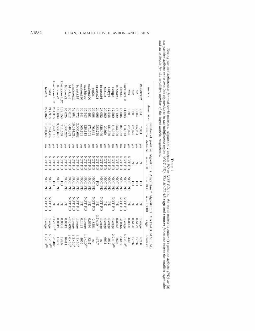
We tested the proposed algorithm for testing positive definiteness on real-worldmatrices from the University of Florida Sparse Matrix Collection [11], selecting varioussymmetric matrices. We use m = 50 and three choices for n: n = 200, 1800, 16000.The results are reported in Table 1. We observe that the algorithm is always correctwhen declaring positive definiteness, but seems to declare indefiniteness when thematrix is too ill-conditioned for it to detect definiteness correctly. In addition, withtwo exceptions (crankseg 1 and pwtk), when n = 16000 the algorithm was correctin declaring whether the matrix is positive definite or not. We remark that whilen = 16000 is rather large it is still smaller than the dimension of most of the matricesthat were tested (recall that our goal was to develop an algorithm that requires asmall number of matrix products, i.e., it does not grow with respect to the matrixdimension). We also note that even when the algorithm fails it still provides usefulinformation about both positive definiteness and the condition number of an inputmatrix, while standard methods such as Cholesky decomposition (as mentioned in
A1582 I. HAN, D. MALIOUTOV, H. AVRON, AND J. SHIN
Table
1T
estingpositive
definitenessfor
real-world
matrices.
Algorithm
7outputs
PD
orN
OT
PD
,i.e.,
theinput
matrix
iseither
(1)positive
definite(P
D)
or(2)
notpositive
definiteor
itssm
allesteigenvalue
isin
theindiff
erenceregion
(NO
TP
D).
The
MA
TL
AB
eigs
andcondest
functionsoutput
thesm
allesteigenvalue
andan
estimate
forthe
conditionnum
berof
theinput
matrix,
respectively.
matrix
dimension
numb
erof
nonzerosp
ositivedefinite
Algorithm
7n
=200
Algorithm
7n
=1800
Algorithm
7n
=16000
MA
TL
AB
eigs
MA
TL
AB
condest
Chem97ZtZ
2,5417,361
yesP
DP
DP
Ddiverge
462.6fv1
9,60485,264
yesP
DP
DP
D0.5122
12.76fv2
9,80187,025
yesP
DP
DP
D0.5120
12.76fv3
9,80187,025
yesN
OT
PD
NO
TP
DP
D0.0020
4420CurlCurl0
11,083113,343
noN
OT
PD
NO
TP
DN
OT
PD
diverge6.2×
1021
barth5
15,606107,362
noN
OT
PD
NO
TP
DN
OT
PD
-2.106684292
Dubcova1
16,129253,009
yesN
OT
PD
NO
TP
DP
D0.0048
2624cvxqp3
17,500114,962
noN
OT
PD
NO
TP
DN
OT
PD
diverge2.2×
1016
bodyy4
17,546121,550
yesN
OT
PD
NO
TP
DP
Ddiverge
1017t3dle
20,36020360
yesN
OT
PD
NO
TP
DP
Ddiverge
6031bcsstm36
23,052320,060
noN
OT
PD
NO
TP
DN
OT
PD
diverge∞
crystm03
24,696583,770
yesN
OT
PD
PD
PD
3.7×10−
15
467.7aug2d
29,00876,832
noN
OT
PD
NO
TP
DN
OT
PD
-2.8281∞
wathen100
30,401471,601
yesN
OT
PD
NO
TP
DP
D0.0636
8247aug3dcqp
35,543128,115
noN
OT
PD
NO
TP
DN
OT
PD
diverge4.9×
1015
wathen120
36,441565,761
yesN
OT
PD
NO
TP
DP
D0.1433
4055bcsstk39
46,7722,060,662
noN
OT
PD
NO
TP
DN
OT
PD
diverge3.1×
108
crankseg1
52,80410,614,210
yesN
OT
PD
NO
TP
DN
OT
PD
diverge2.2×
108
blockqp1
60,012640,033
noN
OT
PD
NO
TP
DN
OT
PD
-446.6368.0×
105
Dubcova2
65,0251,030,225
yesN
OT
PD
NO
TP
DP
D0.0012
10411thermomechTC
102,158711,558
yesN
OT
PD
PD
PD
0.0005125.5
Dubcova3
146,6893,636,643
yesN
OT
PD
NO
TP
DP
D0.0012
11482thermomechdM
204,3161,423,116
yesN
OT
PD
PD
PD
9.1×10−
7125.487
pwtk
217,91811,524,432
yesN
OT
PD
NO
TP
DN
OT
PD
diverge5.0×
1012
bmw32
227,36211,288,630
noN
OT
PD
NO
TP
DN
OT
PD
diverge1.2×
1020

APPROXIMATING SPECTURAL SUMS A1583
subsection 4.6) are intractable for large matrices. Furthermore, one can first run analgorithm to estimate the condition number, e.g., the MATLAB condest function,and then choose an appropriate degree n. We also run the MATLAB eigs function,which is able to estimate the smallest eigenvalue using iterative methods [26] (hence,it can be used for testing positive definitenesss). Unfortunately, the iterative methodoften does not converge, i.e., residual tolerance may not go to zero, as reported inTable 1. One advantage of our algorithm is that it does not depend on a convergencecriterion.
6. Conclusion. Recent years have a seen a surge in the need for various compu-tations on large-scale unstructured matrices. The lack of structure poses a significantchallenge for traditional decomposition based methods. Randomized methods are anatural candidate for such tasks as they are mostly oblivious to structure. In thispaper, we proposed and analyzed a linear-time approximation algorithm for spectralsums of symmetric matrices, where the exact computation requires cubic-time in theworst case. Furthermore, our algorithm is very easy to parallelize since it requires only(separable) matrix-vector multiplications. We believe that the proposed algorithm willfind important theoretical and computational roles in a variety of applications rangingfrom statistics and machine learning to applied science and engineering.
Acknowledgments. The authors thank Peder Oslen and Sivan Toledo for help-ful discussions.
REFERENCES
[1] E. Aune, D. Simpson, and J. Eidsvik, Parameter estimation in high dimensional Gaussiandistributions, Stat. Comput., 24 (2014), pp. 247–263.
[2] H. Avron and S. Toledo, Randomized algorithms for estimating the trace of an implicitsymmetric positive semi-definite matrix, J. ACM, 58 (2011), p. 8.
[3] Z. Bai, G. Fahey, and G. Golub, Some large-scale matrix computation problems, J. Comput.Appl. Math., 74 (1996), pp. 71–89, https://doi.org/10.1016/0377-0427(96)00018-0, http://www.sciencedirect.com/science/article/pii/0377042796000180.
[4] C. Bekas, E. Kokiopoulou, and Y. Saad, An estimator for the diagonal of a matrix, Appl.Numer. Math., 57 (2007), pp. 1214–1229.
[5] J. P. Berrut and L. N. Trefethen, Barycentric Lagrange interpolation, SIAM Rev., 46(2004), pp. 501–517.
[6] C. Boutsidis, P. Drineas, P. Kambadur, and A. Zouzias, A Randomized Algorithm forApproximating the Log Determinant of a Symmetric Positive Definite Matrix, preprintarXiv:1503.00374, 2015.
[7] R. Carbo-Dorca, Smooth function topological structure descriptors based on graph-spectra, J.Math. Chem., 44 (2008), pp. 373–378.
[8] J. Chen, How accurately should I compute implicit matrix-vector products when applying theHutchinson trace estimator?, SIAM J. Sci. Comput., 38 (2016), pp. A3515–A3539, https://doi.org/10.1137/15M1051506.
[9] M. Dashti and A. M. Stuart, Uncertainty quantification and weak approximation of anelliptic inverse problem, SIAM J. Numer. Anal., 49 (2011), pp. 2524–2542.
[10] J. Davis, B. Kulis, P. Jain, S. Sra, and I. Dhillon, Information-theoretic metric learning,in Proceedings of the 24th International Conference on Machine Learning, Corvallis, OR,2007.
[11] T. A. Davis and Y. Hu, The University of Florida sparse matrix collection, ACM Trans. Math.,Software (TOMS), 38 (2011), pp. 1–25, http://www.cise.ufl.edu/research/sparse/matrices.
[12] J. A. de la Pena, I. Gutman, and J. Rada, Estimating the Estrada index, Linear AlgebraAppl., 427 (2007), pp. 70–76.
[13] A. P. Dempster, Covariance selection, Biometrics, (1972), pp. 157–175.[14] E. Di Napoli, E. Polizzi, and Y. Saad, Efficient estimation of eigenvalue counts in an
interval, Numer. Linear Algebra Appl., 23 (2016), pp. 674–692.
A1584 I. HAN, D. MALIOUTOV, H. AVRON, AND J. SHIN
[15] E. Estrada, Characterization of 3D molecular structure, Chemical Physics Letters, 319 (2000),pp. 713–718.
[16] E. Estrada, Topological structural classes of complex networks, Phys. Rev. E, 75 (2007),p. 016103.
[17] E. Estrada, Atom–bond connectivity and the energetic of branched alkanes, Chemical PhysicsLetters, 463 (2008), pp. 422–425.
[18] E. Estrada and N. Hatano, Statistical-mechanical approach to subgraph centrality in complexnetworks, Chemical Physics Letters, 439 (2007), pp. 247–251.
[19] E. Estrada and J. A. Rodrıguez-Velazquez, Spectral measures of bipartivity in complexnetworks, Phys. Rev. E, 72 (2005), p. 046105.
[20] S. A. Gershgorin, Uber die abgrenzung der eigenwerte einer matrix, Izvestiya or RussianAcademy of Sciences, (1931), pp. 749–754.
[21] G. H. Golub and C. F. Van Loan, Matrix Computations, Vol. 3, JHU Press, 2012.[22] I. Gutman, H. Deng, and S. Radenkovic, The Estrada index: An updated survey, Selected
Topics on Appl. Graph Spectra, Math. Inst., Beograd, (2011), pp. 155–174.[23] N. Higham, Functions of Matrices, Society for Industrial and Applied Mathematics, Philadel-
phia, PA, 2008, https://doi.org/10.1137/1.9780898717778.[24] C. Hsieh, M. A. Sustik, I. S. Dhillon, P. K. Ravikumar, and R. Poldrack, BIG & QUIC:
Sparse inverse covariance estimation for a million variables, in Adv. Neural Inf. Process.Syst., 26 (2013), pp. 3165–3173.
[25] M. Hutchinson, A stochastic estimator of the trace of the influence matrix for Laplaciansmoothing splines, Commun. Statistics-Simulation Comput., 19 (1990), pp. 433–450.
[26] I. C. Ipsen, Computing an eigenvector with inverse iteration, SIAM Rev., 39 (1997),pp. 254–291.
[27] V. Kalantzis, C. Bekas, A. Curioni, and E. Gallopoulos, Accelerating data uncertaintyquantification by solving linear systems with multiple right-hand sides, Numer., Algorithms,62 (2013), pp. 637–653.
[28] P. Klein and H.-I. Lu, Efficient approximation algorithms for semidefinite programs arisingfrom max cut and coloring, in Proceedings of the 28th Annual ACM Symposium on The-ory of Computing, Philadelphia, PA, 1996, pp. 338–347, https://doi.org/10.1145/237814.237980.
[29] J. Ma, J. Peng, S. Wang, and J. Xu, Estimating the partition function of graphical modelsusing Langevin importance sampling, in Proceedings of the 16th International Conferenceon Artificial Intelligence and Statistics, Scottsdale, AZ 2013, pp. 433–441.
[30] A. Majumdar and R. K. Ward, An algorithm for sparse MRI reconstruction by Schattenp-norm minimization, Magnetic Resonance Imaging, 29 (2011), pp. 408–417.
[31] D. M. Malioutov, J. K. Johnson, and A. Willsky, Low-rank variance estimation in large-scale GMRF models, in IEEE Int. Conf. on Acoustics, Speech and Signal Processing, Vol.3, Toulouse, FR 2006, pp. III–III.
[32] J. C. Mason and D. C. Handscomb, Chebyshev Polynomials, CRC Press, Boca Raton, FL,2002.
[33] N. Moraca, Bounds for norms of the matrix inverse and the smallest singular value, LinearAlgebra Appl., 429 (2008), pp. 2589–2601.
[34] F. Nie, H. Huang, and C. Ding, Low-rank matrix recovery via efficient Schatten p-norm min-imization, in Proceedings of the 26th AAAI Conference on Artificial Intelligence, Toronto,ON, 2012, pp. 655–661, http://dl.acm.org/citation.cfm?id=2900728.2900822.
[35] R. K. Pace and J. P. LeSage, Chebyshev approximation of log-determinants of spatial weightmatrices, Comput. Statist. Data Anal., 45 (2004), pp. 179–196.
[36] C. E. Rasmussen and C. Williams, Gaussian Processes for Machine Learning, MIT Press,Cambridge, MA, 2005.
[37] F. Roosta-Khorasani and U. M. Ascher, Improved bounds on sample size for implicit matrixtrace estimators, Found. Comput. Math., 15 (2015), pp. 1187–1212, https://doi.org/10.1007/s10208-014-9220-1.
[38] H. Rue and L. Held, Gaussian Markov Random Fields: Theory and Applications, CRC Press,Boca Raton, FL, 2005.
[39] A. Stathopoulos, J. Laeuchli, and K. Orginos, Hierarchical probing for estimating the traceof the matrix inverse on toroidal lattices, SIAM J. Sci. Comput., 35 (2013), pp. S299–S322.
[40] M. L. Stein, J. Chen, and M. Anitescu, Stochastic approximation of score functions forGaussian processes, Annals Appl. Statist., 7 (2013), pp. 1162–1191.
[41] T. Tao and V. Vu, Random matrices: The distribution of the smallest singular values, Geom.Funct. Anal., 20 (2010), pp. 260–297.
[42] T. Tao and V. H. Vu, Inverse Littlewood-Offord theorems and the condition number of randomdiscrete matrices, Ann. Math., 169 (2009), pp. 595–632.
APPROXIMATING SPECTURAL SUMS A1585
[43] L. N. Trefethen, Approximation Theory and Approximation Practice, Society for Industrialand Applied Mathematics, Philadelphia, PA, 2012.
[44] S. Van Aelst and P. Rousseeuw, Minimum volume ellipsoid, Wiley Interdisciplinary Reviews:Computational Statistics, 1 (2009), pp. 71–82.
[45] M. J. Wainwright and M. I. Jordan, Log-determinant relaxation for approximate in-ference in discrete Markov random fields, IEEE Trans. Signal Process., 54 (2006),pp. 2099–2109.
[46] L. Wu, J. Laeuchli, V. Kalantzis, A. Stathopoulos, and E. Gallopoulos, Estimating thetrace of the matrix inverse by interpolating from the diagonal of an approximate inverse, J.Comput. Phys., 326 (2016), pp. 828–844, https://doi.org/10.1016/j.jcp.2016.09.001, http://www.sciencedirect.com/science/article/pii/S0021999116304120.
[47] S. Xiang, X. Chen, and H. Wang, Error bounds for approximation in Chebyshev points,Numer. Math., 116 (2010), pp. 463–491.
[48] Y. Zhang and W. E. Leithead, Approximate implementation of the logarithm of the ma-trix determinant in Gaussian process regression, J. Stat. Comput. Simul., 77 (2007),pp. 329–348.