Approximation Algorithms for Finding Low-DegreeSubgraphs

Philip N. KleinDepartment of Computer Science, Box 1910, Brown University, Providence, Rhode Island 02912-1910

Radha Krishnan and Balaji RaghavachariDepartment of Computer Science, University of Texas at Dallas, Richardson, Texas 75080-0688

R. RaviTepper School of Business, Carnegie Mellon University, Schenley Park,Pittsburgh, Pennsylvania 15213-3890

We give quasipolynomial-time approximation algorithmsfor designing networks with a minimum degree. Usingour methods, one can design networks whose connec-tivity is specified by “proper” functions, a class of 0–1functions indicating the number of edges crossing eachcut. We also provide quasipolynomial-time approxima-tion algorithms for finding two-edge-connected span-ning subgraphs of approximately minimum degree of agiven two-edge-connected graph, and a spanning tree(branching) of approximately minimum degree of a di-rected graph. The degree of the output network in allcases is guaranteed to be at most (1 � �) times theoptimal degree, plus an additive O(log1��n) for any � > 0.Our analysis indicates that the degree of an optimalsubgraph for each of the problems above is well esti-mated by certain polynomially solvable linear programs.This suggests that the linear programs we describecould be useful in obtaining optimal solutions via branchand bound. © 2004 Wiley Periodicals, Inc. NETWORKS, Vol.44(3), 203–215 2004

Keywords: approximation algorithms; minimum-degree sub-graphs; graph algorithms; network design; graph connectivity; NP-hard problems

1. INTRODUCTION

Minimizing the maximum degree is desirable in commu-nications networks. The advantage of a network with a lowmaximum degree is that the failure of a single node does notresult in adverse conditions for a large part of the network.Keeping the maximum degree small is also essential indesigning switching networks with identical switches in-stalled at all nodes. In this case, switches for the networkneed to be designed to handle as many connections as themaximum degree of any node. Minimum-degree networksare also useful in building networks for broadcast where wewish to minimize the amount of work done at each site, andalso in designing power grids where the cost of a nodeincreases with the degree of splitting the power [6]. Thus,the very nature of the network itself gives rise to certainconnectivity requirements in the network. In this article, westudy algorithms for designing such low-degree communi-cations networks.

The following versions of the basic minimum-degreesubgraph problems are considered.

1. Network design problems where the connectivity re-quirements can be modeled by a {0, 1}-valued functionf on all the cuts in the graph. This framework is generalenough to capture the Steiner and generalized Steinertree problems.

2. Two-edge-connected spanning subgraph of a givengraph.

3. Spanning trees in directed graphs.

In each case, the goal is to find, for the given graph, aminimum-degree subgraph that satisfies the given connec-tivity constraints. We provide approximation algorithmsthat output networks in each case, whose degrees are guar-

Received November 2002; accepted May 2004Correspondence to: B. Raghavachari; e-mail: rbk@utdallas.eduContract grant sponsor: NSF; contract grant number: CCR-9012357 (toP.N.K.)Contract grant sponsor: NSF PYI award; contract grant number: CCR-9157620 (to P.N.K. and R.R.)Contract grant sponsor: DARPA; contract grant number: N 0014-91-J-4052 (ARPA order No. 8225, to P.N.K. and R.R.)Contract grant sponsor: NSF; contract grant number: CCR-9820902 (to B.R.)Contract grant sponsor: IBM grant fellowship (to R.R.)DOI 10.1002/net.20031Published online in Wiley InterScience (www.interscience.wiley.com).© 2004 Wiley Periodicals, Inc.

NETWORKS—2004

anteed to be at most (1 � �) times optimal, plus an additiveterm of O(log1��n) for any � � 0. The algorithms run inquasipolynomial time O(nlog1��n). As a direct consequence,we obtain polynomial-time approximation algorithms for allproblems above with a performance ratio O(n1/�) for any �� 0 (by setting � � n�). In addition to the same perfor-mance guarantees and running times, all the algorithms wedescribe here also have in common the technique of localoptimization, wherein we perform local improvements tothe current solution to iteratively decrease the degrees ofhigh-degree nodes.

In Section 2, we review previously known results forspecial cases of the problems we consider in this article. InSection 3, we describe our results on general minimum-degree one-connected networks. In Section 4, we addressthe minimum-degree two-edge-connected spanning net-work-design problem. The directed minimum-degree span-ning tree problem is considered in Section 5.

2. PREVIOUS WORK

2.1. The Basic Minimum-Degree Spanning Tree (MDST)Problem

Given an undirected graph G, the problem is to find aspanning tree of G whose maximum degree is minimal. Thisproblem is a generalization of the Hamiltonian Path prob-lem, and hence, is NP-hard [9]. Furer and Raghavachari [5]gave a polynomial-time approximation algorithm for thisproblem with O(log n) performance guarantee. In subse-quent work [6], they improved their previous results andprovided another polynomial-time algorithm to approximatethe minimum-degree spanning tree to within 1 of the opti-mal. Clearly, no better approximation algorithms are possi-ble for this problem.

Lawler [16] showed that matroid methods sufficed tosolve the following variant of the minimum-degree span-ning tree problem in polynomial time: given a graph G andan independent set I of nodes of G, find a spanning tree thatminimizes the maximum degree of any node in I. Gavish[10] formulated the minimum-degree spanning tree problemas a mixed-integer program and provided an exact solutionusing the method of Lagrangian multipliers.

2.2. The Minimum-Degree Steiner Tree Problem

In this extension to the MDST problem, given an inputgraph and a distinguished subset of the nodes D, we seek tofind a Steiner tree (spanning at least the set D) whosemaximum degree is minimum. The first polynomial-timeapproximation algorithm was provided by Agrawal, Klein,and Ravi [1]. The performance guarantee is a factor ofO(log k), where k is the size of D. This was improved uponby Furer and Raghavachari [6], who provide a polynomial-time approximation algorithm for the problem. Their per-formance guarantee is essentially the same as that shown by

us. In fact, our work is a generalization of their algorithm,and reduces to their algorithm for this special case. Furerand Raghavachari [7] later demonstrated a polynomial-timealgorithm that finds a tree whose degree is within 1 fromoptimal.

2.3. The Directed Minimum-Degree Spanning TreeProblem

Given a directed graph G and a root node r � V, theproblem is to find a spanning tree of G rooted at r whosemaximum degree is minimized. For this problem, Furer andRaghavachari [5] gave an algorithm with an approximationratio of O(log n) for this problem. Our article improves themultiplicative factor of O(log n) to an additive term ofO(log n). Unfortunately, the “plus one” algorithm [7] doesnot generalize to directed graphs.

3. THE MINIMUM-DEGREE CONSTRAINEDFOREST PROBLEM

We begin this section by describing a framework forformulating general one-connected network problems. Weformulate the minimum degree problem in this framework.

3.1. Formulation

A framework for specifying connectivity requirementsfor networks was proposed by Goemans and Williamson[11]. This framework captures a wide variety of requirementspecifications, including Steiner and generalized Steinerconnectivity, general point-to-point connectivity, and T-joins. Building on the work of Agrawal, Klein, and Ravi onthe generalized Steiner tree problem [2], Goemans andWilliamson showed a way to find a network satisfying givenconnectivity requirements that has nearly minimum totaledge cost. In this article, we show how to find a networksatisfying the requirements that has nearly minimum de-gree. We use the framework from [11] for specifying con-nectivity requirements. Our algorithm and analysis arebased on the work of Furer and Raghavachari [6].

Consider a spanning tree of a graph, and any cut in thegraph. At least one edge of the spanning tree must cross thiscut. Conversely, if a network crosses every cut, it must spanall nodes. More generally, to specify connectivity require-ments for a network, we designate a subset of the cuts in agraph as active cuts, and we require that the network beingdesigned cross every active cut.

A broad class of requirements can be specified using anapproach of Goemans and Williamson [11]. They specifywhich cuts are active using a 0–1 function f on the node-subsets of a graph. For a node-subset S, let �(S) denote theset of edges each having exactly one endpoint in S. Tospecify that the cut �(S) is active, we set f(S) to be 1. Onecan now formulate an integer program for a minimum-degree network crossing all active cuts:

204 NETWORKS—2004

Min d

subject to constraints:

x���S�� � f�S� � S � V

x����v��� � d � v � V (IP)

xe � �0, 1� � e � E

Here, for any subset F of edges, x(F) is defined to be ¥e�F

xe. We call any feasible solution to the above IP, an f-join.It is easy to verify that minimal f-joins are forests.

Goemans and Williamson [11] focus on a special class offunctions f that can be used to formulate many importantconnectivity requirements. They called these functionsproper. A function f : 2V 3 {0, 1} is proper if thefollowing properties hold.

1. [Null] f(A) � 0;2. [Symmetry] f(S) � f(V S) for all S � V; and3. [Disjointness] If A and B are disjoint, then f( A) � f(B)

� 0 implies f( A � B) � 0.

We are interested in solutions to (IP) for the class of properfunctions f. Examples of problems that fit within this frame-work other than the minimum-degree Steiner trees are min-imum-degree generalized Steiner forests, minimum-degreeT-joins, and minimum-degree point-to-point connectionproblems.

3.2. Preliminaries: Toughness, Weakness and LowerBounds

Toughness, first defined by Chvatal in [4], is a measureof how hard it is to disconnect a graph into many compo-nents by removing a small number of nodes. The toughnessof a graph is the minimum (over all nontrivial node subsets)of the ratio of the number of nodes removed (X) to thenumber of connected components in the remaining graph.That is, it is the minimum of all ratios of �X� to the numberof components in G X, where X ranges over all nontrivialnode subsets of G. Computing the toughness of a graph wasshown to be NP-complete by Bauer, Hakimi, andSchmeichel [3]. Win [20] has shown the following interest-ing relationship between the toughness of a graph and theminimum-degree spanning tree problem. He showed that ifthe toughness of a graph is at least 1/(k 2), then it has aspanning tree whose degree is at most k (for k � 2).

The definition of toughness we have given differsslightly from Chvatal’s original definition in [4]. Accordingto our definition, the minimum toughness ratio is nevermore than 1 (for nonsingleton graphs), because even asingleton X yields a ratio of at most 1. Chvatal definestoughness to be the same minimum ratio, but the minimumis taken only over those node subsets X for which G X

has at least two components. According to this definition,the minimum ratio can be arbitrarily large.

We generalize the above notion to allow active compo-nents defined by proper functions f. For any X � V, aconnected component Y of G X is active under a properfunction f whenever f(Y) � 1. The f-toughness of a graphfor any given function f is the minimum ratio of the numberof nodes removed to the number of active componentsformed. In other words, it is the minimum ratio of �X� to thenumber of active components in G X, where X rangesover all nontrivial node subsets of G. For any subset X ofnodes, this ratio is termed the f-toughness of the set X. Thus,the f-toughness of the graph is the minimum f-toughness ofany of its nontrivial node subsets. Note that ordinary tough-ness is a special case of f-toughness as we have defined it,because it corresponds to a function f where every nontrivialsubset of the nodes of the graph is active. We are interestedin computing the f-toughness of the graph for proper func-tions f. Call any single node that forms an active set aterminal. Note that as long as there is at least one terminal,the f-toughness ratio is at most 1, because this is the ratioachieved on removing a single terminal.

We shall refer to the reciprocal of the f-toughness of agraph as its f-weakness. The notion of weakness of a grapharises as a dual to the problem of constructing minimum-degree networks. The f-weakness of the graph is an estimateof the vulnerability of any f-join. A node subset with highvalue of f-weakness represents a weak spot in such a net-work: damage to this subset results in nearly the worstdisconnection among the nodes in the network. To motivatethe relationship between the minimum degree of any f-joinand the f-weakness, we prove the following lemma.

Lemma 3.1. For any function f, the optimum value of (IP)is at least the f-weakness of the graph.

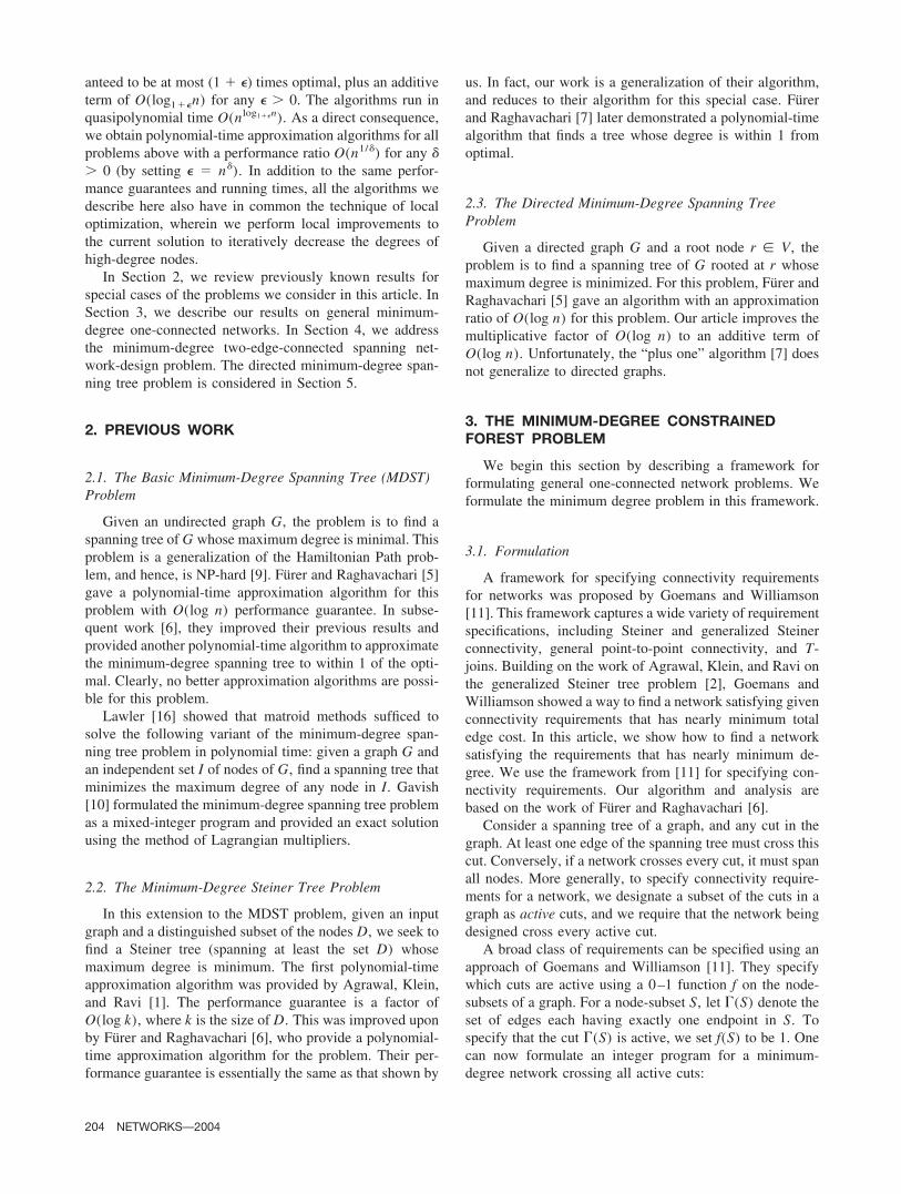
Proof. Consider the node set X achieving the optimalf-weakness (see Fig. 1). Let the number of active compo-nents in G X under f be k. In any f-join, each of the kactive components in G X must have an edge to X. Thus,

FIG. 1. f-weakness is a lower bound on the maximum degree of an f-join.In a feasible f-join, the degree of nodes in X is at least ratio of number ofactive components created on deleting X to the cardinality of X.

NETWORKS—2004 205

the average degree (and, hence, the maximum degree) of anode of X in an optimal solution to (IP) is at least k/�X�, thef-weakness of the graph. ■

3.3. The Algorithm and Its Analysis

We now describe the algorithm for providing an approx-imate solution to (IP) and analyze its performance. As inputwe are given an undirected graph G � (V, E), an arbitrarynumber � � 0 to determine the performance accuracy, anda proper function f defined on the cuts of G. We can assumewithout loss of generality that the graph G is connected, forotherwise we can work on each connected component of Gindependently. Our algorithm uses iterative local improve-ments and outputs a forest F that is feasible for the coveringconstraints of (IP). Note that we can always assume withoutloss of generality that any feasible solution to (IP) is theincidence vector of a forest [11]. Feasible solutions satisfythe following lemma.

Lemma 3.2 ([12]). Let F denote a subset of the edge set ofG. F is a feasible solution to (IP) if and only if f(N) � 0 foreach connected component N of F.

3.3.1. OverviewThe algorithm starts with a feasible solution to (IP) and

iteratively applies improvement steps aimed at reducing thedegree of high-degree nodes. Intuitively, if we find a cyclein the graph that contains a node w of high degree, and if alledges that must be added to the current feasible solution toform this cycle are incident to low-degree nodes, then wecan improve the current solution by adding in the cycle anddeleting an edge incident to w. This reduces the degree of wby 1. For minimum-degree spanning trees [6, 7], improve-ments consisted of simply replacing one edge by another,and in the case of Steiner trees, they were defined asreplacing an edge by a path whose internal nodes are not inthe tree. Therefore, the degree of nodes in the tree increasedby at most 1. In our case, we are replacing an edge by acollection of paths that could go through nodes in othertrees. Therefore, the degree of a node may increase by twoafter an improvement. We examine this in greater detailbelow.

3.3.2. An Improvement StepLet Sd denote the set of nodes in the current forest whose

degree is at least d. An improvement step with target d triesto reduce the degree of a node in Sd. We use two types ofimprovement steps. The first and simpler type determineswhether the forest F remains feasible on deleting an edgeincident on a node in Sd. If so, we delete this edge from Fto obtain the new forest F and proceed to the next im-provement step. The second type of improvement step ismore involved. Starting from G, we delete all the edges inE F that are incident to nodes in the forest having degreeat least d 2, i.e., edges that are incident to nodes in Sd2.In this graph, we examine if any node in Sd lies on a cycle.

If so, we add all the edges in E F in this cycle to theforest F and delete an edge of F incident to a node in Sd inthis cycle. If any other cycles have been created, removesome of the added edges to make the solution acyclic. Thisgives a new forest F.

Note that after performing an improvement step withtarget d, the degree of a node in Sd reduces by one and theresulting degree of each of the affected nodes increases byat most 2 and is at most d 1. We note that the resultingforest F is an f-join.

Lemma 3.3. The forest F formed at the end of an im-provement step remains feasible.

Proof. The lemma follows immediately if the improve-ment step is of the first type. Therefore, suppose the im-provement is of the second type. Let F be the feasible forestbefore the improvement step. Consider the cycle involved inthe improvement. Because F is acyclic, the addition of thecycle and the deletion of an edge clearly leaves F acyclic.But, we have merged many of the trees in F to form a singletree containing the edges of the cycle in F. However,because F was feasible, Lemma 3.2 guarantees that each ofthe trees in the merged tree has f-value 0. Because themerged component is a disjoint union of these components,the disjointness property of f implies that the f value of thisnew component is also 0. All the remaining components inF were also components of F having f-value 0. Therefore,Lemma 3.2 implies that F is feasible. ■

3.3.3. The AlgorithmThe algorithm starts with an initial feasible solution. Any

spanning tree T of the given connected graph can be chosenas the initial feasible solution. Note that the null and sym-metry conditions on f imply that f(V) � 0 and so, byLemma 3.2, T is feasible. Let the maximum degree of anynode in the current feasible solution be k. Ideally, we wouldlike to run the algorithm until no further improvements arepossible. Unfortunately, we are unable to bound the runningtime of such an algorithm even using a quasipolynomialterm. Therefore, we restrict improvements only when theyapply to high-degree nodes. The algorithm applies improve-ment steps with target d for d � k 2 log1��n until nosuch improvements are possible. The resulting forest isoutput as a locally optimal approximate solution.

Definition 3.4. Define an edge e of a feasible forest F tobe critical if F e is not feasible.

As a result of performing the first type of improvementstep, note that all the edges incident on nodes of degree atleast k 2 log1��n are critical in the locally optimalsolution.

3.3.4. TerminationEach improvement step is polynomial-time implement-

able. We adapt a potential-function argument from [6] to

206 NETWORKS—2004

bound the number of improvement steps. We define thepotential of a node v with degree d in the forest F to be �(v)� nd where n is the number of nodes in the graph. Thepotential of the forest F is defined as �(F) � ¥v �(v).Initially �(F) � nn. Each improvement step with target dreduces the potential by at least (n 1)nd3, because thedegree of a node of degree d is reduced by 1 and the degreeof all the other nodes may increase to d 1. Because d � k 2 log1��n where k is the maximum degree of thecurrent forest, this reduction in potential is at least a fractionn2 log1��n3 of the current potential of the forest �(F).From this we can bound the maximum number of iterationsbefore k decreases, and k can decrease at most n 3 times.It follows that the number of improvement steps is at mostnO(log1��n).

3.3.5. Performance GuaranteeWe prove the performance guarantee by identifying a

node separator from the solution subgraph whose f-weak-ness value is very close to the degree of the solution. Let kdenote the maximum degree of the solution subgraph. Asimple contradiction argument proves the following propo-sition.

Proposition 3.5. There is some i � [k 2 log1��n , k]with �Si2� � (1 � �)�Si�.

In the following discussion, let i be an index that satisfiesthe above proposition. We prove the following criticallemma that shows that when Si2 (the set of nodes ofdegree at least i 2 in a locally optimal solution) is deletedfrom G, a large number of active components are created.This will then imply that the degree of nodes in Si2 has tobe large in any solution, because all these active compo-nents in G Si2 can be connected together in a feasiblesolution only using edges that are incident to some node ofSi2. The reason why our analysis is more complicated thanthe one used for minimum-degree Steiner trees is due to thefact that our feasible solution may have several trees, andtherefore, there may be edges in the graph that connecttogether some of these active components that are not usefulin any improvements. But we show that the number of suchcomponents that may be merged with other components aresmall, and we can account for them in our analysis.

Lemma 3.6. Let F be the locally optimal network and leti be the index in Proposition 3.5. The number of activecomponents in G Si2 is at least i�Si� (2 � �)�Si�.

We prove the above lemma in the remainder of thissection. Call a tree in F relevant if it contains a node in Si.Define an equivalence relation � on the edges of F by therule: e1 � e2 if there is a path between an endpoint of e1

and an end point of e2 in F avoiding Si. Intuitively, anequivalence class under this relation is a set of edges inci-dent to nodes whose degree is smaller than i, forming aconnected subtree in F. We define a bipartite graph that

captures the way in which these subtrees are connected tonodes of Si as follows. Define an auxiliary forest Fi whosenodes are Si together with the equivalence classes of �. Fi

has an edge between a node v � Si and an equivalence classC under � if there is an edge in C incident on v. Note thatbecause F is acyclic, there is at most one edge in anyequivalence class C incident to any node v in Si. Thus, if anode v � Si has degree j in F, it also has degree j in Fi.Note also that Fi is acyclic and has exactly as many com-ponents as the number of relevant trees in F. We areespecially interested in the leaves of Fi, i.e., subtrees of Fthat have a single edge of F that connects them to somenode in Si. We show a lower bound on the number of suchsubtrees.

Claim 3.7. The number of nodes of degree one in Fi

(corresponding to equivalence classes C) is at least (i 2)�Si� � 2r where r is the number of relevant trees in F.

Proof. Let t be the number of classes of degree 1 andlet p be the number of other classes. The number of edgesin the forest Fi is the number of nodes in the forest minusthe number of components in it. This is exactly t � p � �Si� r. The sum of the degrees of the nodes of Fi is twice thenumber of edges. That sum is at least i � �Si� � 2p � t. Theclaim follows. ■

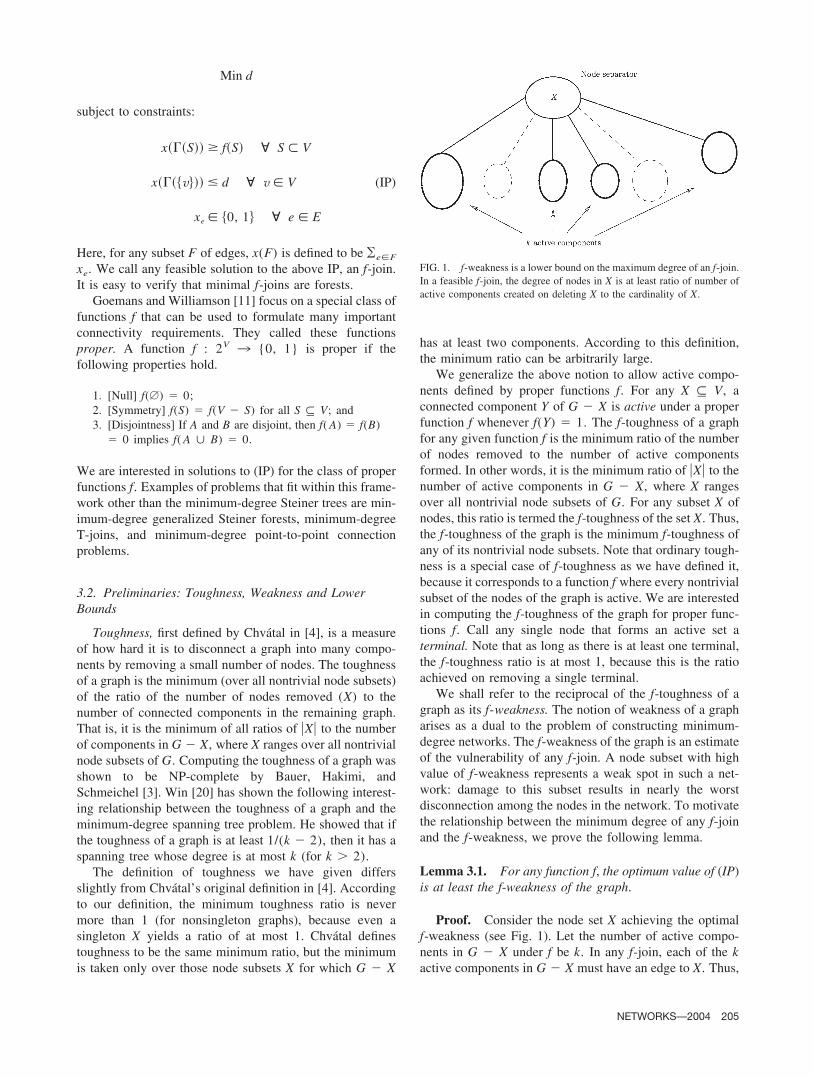
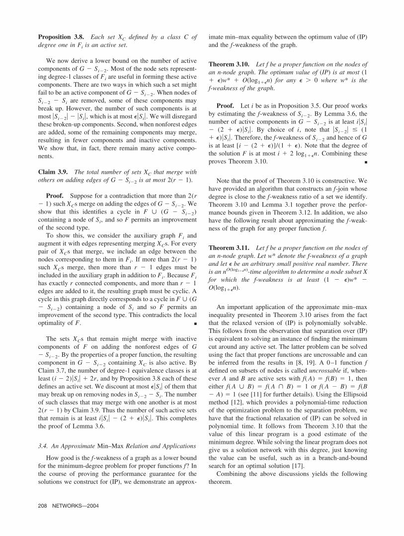
Each class C of degree one defines a set XC of nodes asfollows: a node v is in XC if C contains all the edges of Fthat are incident on v. Note that each XC is a component ofF Si and thus represents a subset of nodes of a relevanttree (see Fig. 2). Consider an edge e in F incident on a nodein Si. Because F is feasible, by Lemma 3.2, the componentof F containing e is inactive. Because e is critical onaccount of the first type of improvement step, the twodistinct components formed in F on removing e and con-taining its endpoints must both be active. Consider an edgein a degree-1 equivalence class C of � that is incident on anode in Si. One of the connected components formed on itsremoval from F is XC, and so this set is active. This issummarized in the following proposition.

FIG. 2. Three degree-1 equivalence classes under �, each with an edgeto a node v � Si.

NETWORKS—2004 207

Proposition 3.8. Each set XC defined by a class C ofdegree one in Fi is an active set.

We now derive a lower bound on the number of activecomponents of G Si2. Most of the node sets represent-ing degree-1 classes of Fi are useful in forming these activecomponents. There are two ways in which such a set mightfail to be an active component of G Si2. When nodes ofSi2 Si are removed, some of these components maybreak up. However, the number of such components is atmost �Si2� �Si�, which is at most ��Si�. We will disregardthese broken-up components. Second, when nonforest edgesare added, some of the remaining components may merge,resulting in fewer components and inactive components.We show that, in fact, there remain many active compo-nents.

Claim 3.9. The total number of sets XC that merge withothers on adding edges of G Si2 is at most 2(r 1).

Proof. Suppose for a contradiction that more than 2(r 1) such XCs merge on adding the edges of G Si2. Weshow that this identifies a cycle in F � (G Si2)containing a node of Si, and so F permits an improvementof the second type.

To show this, we consider the auxiliary graph Fi andaugment it with edges representing merging XCs. For everypair of XCs that merge, we include an edge between thenodes corresponding to them in Fi. If more than 2(r 1)such XCs merge, then more than r 1 edges must beincluded in the auxiliary graph in addition to Fi. Because Fi

has exactly r connected components, and more than r 1edges are added to it, the resulting graph must be cyclic. Acycle in this graph directly corresponds to a cycle in F � (G Si2) containing a node of Si and so F permits animprovement of the second type. This contradicts the localoptimality of F. ■

The sets XCs that remain might merge with inactivecomponents of F on adding the nonforest edges of G Si2. By the properties of a proper function, the resultingcomponent in G Si2 containing XC is also active. ByClaim 3.7, the number of degree-1 equivalence classes is atleast (i 2)�Si� � 2r, and by Proposition 3.8 each of thesedefines an active set. We discount at most ��Si� of them thatmay break up on removing nodes in Si2 Si. The numberof such classes that may merge with one another is at most2(r 1) by Claim 3.9. Thus the number of such active setsthat remain is at least i�Si� (2 � �)�Si�. This completesthe proof of Lemma 3.6.

3.4. An Approximate Min–Max Relation and Applications

How good is the f-weakness of a graph as a lower boundfor the minimum-degree problem for proper functions f? Inthe course of proving the performance guarantee for thesolutions we construct for (IP), we demonstrate an approx-

imate min–max equality between the optimum value of (IP)and the f-weakness of the graph.

Theorem 3.10. Let f be a proper function on the nodes ofan n-node graph. The optimum value of (IP) is at most (1� �)w* � O(log1��n) for any � � 0 where w* is thef-weakness of the graph.

Proof. Let i be as in Proposition 3.5. Our proof worksby estimating the f-weakness of Si2. By Lemma 3.6, thenumber of active components in G Si2 is at least i�Si� (2 � �)�Si�. By choice of i, note that �Si2� � (1� �)�Si�. Therefore, the f-weakness of Si2 and hence of Gis at least [i (2 � �)]/(1 � �). Note that the degree ofthe solution F is at most i � 2 log1��n. Combining theseproves Theorem 3.10. ■

Note that the proof of Theorem 3.10 is constructive. Wehave provided an algorithm that constructs an f-join whosedegree is close to the f-weakness ratio of a set we identify.Theorem 3.10 and Lemma 3.1 together prove the perfor-mance bounds given in Theorem 3.12. In addition, we alsohave the following result about approximating the f-weak-ness of the graph for any proper function f.

Theorem 3.11. Let f be a proper function on the nodes ofan n-node graph. Let w* denote the f-weakness of a graphand let � be an arbitrary small positive real number. Thereis an nO(log1��n)-time algorithm to determine a node subset Xfor which the f-weakness is at least (1 �)w* O(log1��n).

An important application of the approximate min–maxinequality presented in Theorem 3.10 arises from the factthat the relaxed version of (IP) is polynomially solvable.This follows from the observation that separation over (IP)is equivalent to solving an instance of finding the minimumcut around any active set. The latter problem can be solvedusing the fact that proper functions are uncrossable and canbe inferred from the results in [8, 19]. A 0–1 function fdefined on subsets of nodes is called uncrossable if, when-ever A and B are active sets with f( A) � f(B) � 1, theneither f( A � B) � f( A � B) � 1 or f( A B) � f(B A) � 1 (see [11] for further details). Using the Ellipsoidmethod [12], which provides a polynomial-time reductionof the optimization problem to the separation problem, wehave that the fractional relaxation of (IP) can be solved inpolynomial time. It follows from Theorem 3.10 that thevalue of this linear program is a good estimate of theminimum degree. While solving the linear program does notgive us a solution network with this degree, just knowingthe value can be useful, such as in a branch-and-boundsearch for an optimal solution [17].

Combining the above discussions yields the followingtheorem.

208 NETWORKS—2004

Theorem 3.12. Let f be a proper function. Let d* denotethe optimum value of (IP). There is an nO(log1��n)-time algo-rithm for finding a feasible solution to (IP) whose objectivevalue is at most (1 � �)d* � O(log1��n) for any � � 0.

4. MINIMUM-DEGREE TWO-EDGE-CONNECTEDSUBGRAPHS

In this section, we consider minimum-degree networksof a different type. Given a two-edge-connected undirectedgraph as input, we consider the problem of finding a two-edge-connected spanning subgraph of minimum degree.This problem can be easily seen to be NP-hard by a reduc-tion from the Hamiltonian cycle problem. Using a local-improvement algorithm similar to that used in proving The-orem 3.12, we obtain an approximate solution for thisproblem as well.

Theorem 4.1. Let �* be the minimum degree of a two-edge-connected subgraph of a given graph G and let � be apositive number. There is an nO(log1��n)-time algorithm forfinding a two-edge-connected subgraph of G having degreeat most (1 � �)�* � O(log1��n).

As in Section 3, it is easy to cast this problem as anexponential-sized integer program. The first constraint ismodified to x(�(S)) � 2 for all S � V. This captures thecondition that our solution needs to have at least two edgesacross each cut, i.e., it is two-edge-connected. The fractionalrelaxation of this program is solvable in polynomial time byusing a minimum-cut procedure to solve the correspondingseparation problem. Hence, the above theorem can be ap-plied to show that this linear program solution value is avery good estimate of the value of the exact solution to theminimum-degree problem. As mentioned earlier, such esti-mates can be used in pruning the search space for exactsolutions to this problem.

4.1. Preliminaries

Let G � (V, E) be an arbitrary k-edge-connected graph.Consider the problem of computing a k-edge-connectedsubgraph N of G, which spans V such that the maximumdegree of N is minimum. The case of k � 1 corresponds tothe minimum-degree spanning tree problem and is NP-hard[10]. In this section, we consider the case when k � 2(two-edge-connected graphs are also called bridge-con-nected). In this article, “connectivity” always stands foredge connectivity (and not node connectivity). For a graphG, we use �*(G) to denote the minimum degree of atwo-connected spanning subgraph of G.

We first give some preliminary definitions that show thatthe notion of k-connected components is meaningful in thecontext of edge connectivity. It allows the partition of V intok-connected components.

Definition 4.2. A pair of nodes u and v is said to bek-connected in a graph N if there are k edge-disjoint pathsbetween u and v in N. This relation is an equivalencerelation. It partitions the nodes into equivalence classes ofnodes. Within each class, each pair of nodes is k-connected.Such a class is called a k-component.

Definition 4.3. For a graph H, the bridge-connected for-est (bcf) of H is obtained by contracting each two-compo-nent of H to a supernode and deleting self-loops. A leaftwo-component of H is a two-component that has degreeone in the bcf of H. An isolated two-component of H is oneof degree zero in the bcf of H.

The following lemma follows from the definition oftwo-edge-connected graphs.

Lemma 4.4. Let N be any two-connected spanning sub-graph of G, and let X be any subset of nodes. Let C be atwo-component of G X. If C is a leaf two-component, thenN has at least one edge between C and X. If C is an isolatedtwo-component, then N has at least two edges between Cand X.

This lemma motivates the following definition.

Definition 4.5. Let H be a graph with � leaf two-compo-nents and k isolated two-components. Then the deficiency ofH is defined as � � 2k and is denoted by def(H).

The stage is now set for an easy derivation of a lowerbound on the minimum degree of a two-connected spanningsubgraph. Consider removing a node subset X from anundirected graph G; the remaining graph has deficiencydef(G X). In any two-connected spanning subgraph ofG, there must be at least def(G X) edges going betweenG X and the nodes in X by Lemma 4.4. Thus, themaximum degree of a node in X is at least [def(G X)]/�X�. Applying this argument to the minimum-degree two-connected spanning subgraph, we arrive at the followingcorollary.

Corollary 4.6. Let X be a subset of the nodes of a graphG. Then

�*�G� �def�G � X�

�X�

4.2. The Algorithm and Its Time Complexity

The local-search algorithm proceeds as follows. We fix �to be any arbitrary quantity greater than zero. The algorithmstarts with an arbitrary two-connected subgraph of the givengraph G, and iteratively applies local improvement steps toreduce the degrees of high-degree nodes. When a local

NETWORKS—2004 209

minimum is reached, the algorithm outputs the current sub-graph.

Now we give definitions pertaining to an improvementstep. Let N denote a two-connected subgraph of G. For anedge e � N, we define Ne to be the bcf of N e. BecauseN is two-connected, it follows that Ne is a simple path.

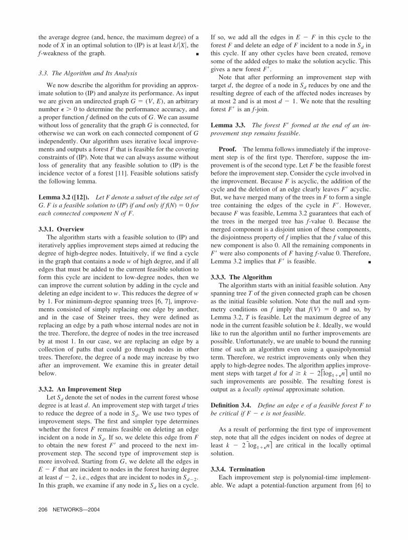
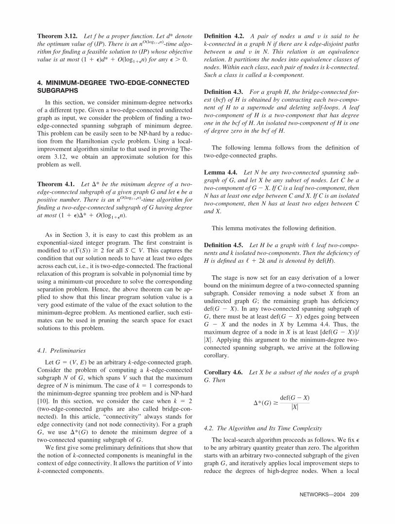
Definition 4.7. The degree-d candidate graph for an edgee in N is obtained from G as follows: contract each two-component of N e, and then delete e and the edges of G N incident to nodes with degree at least d in N (see Fig.3). A node w of degree d in N is said to admit an improve-ment if there is an edge e incident to w in N such that thedegree-(d 3) candidate graph for e is two-connected.

An improvement step consists of replacing e with edgesfrom the candidate graph so that the resulting networkremains two-connected. We require that the degree of nonode is increased beyond d 1. The following lemmashows that this can be done. We use degH(v) to denote thedegree of a node v in the subgraph formed by a collection Hof edges.

Lemma 4.8. Let Q be a minimal collection of edges whoseaddition two-connects a bcf Ne. Then for every node v of Ne,degQ(v) � 2.

Proof. Suppose that degQ(v) � 3. Because Ne is apath, v splits Ne into two subpaths. Then at least two of v’sthree incident edges must be incident on nodes in the samesubpath. Let a be the one whose other endpoint is closer tov in the subpath. Then Q a also two-connects Ne,contradicting the minimality of Q. ■

Note that an improvement step for a node w decreases

w’s degree by 1, but does not increase the degree of anyother node to more than w’s new degree.

Definition 4.9. Let N be a two-connected spanning sub-graph of G, and let � be the degree of N. Then N is calledlocally optimal if no node of degree at least � 2 log1��nadmits an improvement.

Using a potential function argument as in Section 3, it iseasy to show that nO(log1��n) improvement steps suffice toyield a locally optimal subgraph. Because each improve-ment step can be executed in polynomial time, the runningtime is as claimed in Theorem 4.1. In the remainder of thissection, we show that the degree of a locally optimal sub-graph is as claimed in Theorem 4.1.

4.3. Performance Guarantee

Theorem 4.10. The degree of any locally optimal sub-graph of a graph G with n nodes is at most (1 � �)�*(G)� 2 log1��n � 4(1 � �).

Let Si denote the set of nodes whose degree in N is atleast i. The proof of Theorem 4.10 consists in showing thatthere is an i in the range [� 2 log1��n , �] for which G Si has many leaf and isolated two-components. We showthis in Lemma 4.13. Theorem 4.10 then follows from Cor-ollary 4.6.

Lemma 4.11. Let G be a two-connected graph and let Sbe a subset of nodes of G. Then there is a two-connectedsubgraph A of G that contains all nodes of S, such that ¥v�S

degA(v) � 4�S�.

Proof. We give a constructive proof by demonstratingan algorithm to compute A. A graph H is defined to be aminor of graph G if one can obtain H from G by repeatedlycontracting or deleting edges. For a minor H of G, we saya node v of H is active if one of the nodes contracted to formv belongs to S. Consider the following algorithm:

1. Initialize H0 :� G.2. Let j :� 0 and let A0 be the empty graph.3. Although S is not two-connected via Aj, do

a. Let Cj�1 be a shortest cycle in Hj containing at leasttwo active nodes.

b. Let Aj�1 :� Aj � Cj�1.c. Obtain Hj�1 from Hj by contracting together all

nodes of Cj�1.d. j :� j � 1.

Let k be the number of iterations. By the termination con-dition, S is two-connected in Ak. For each j, let xj be thenumber of active nodes in Cj. Because the edges of Cj forma cycle in Hj, the degree increase due to these edges onactive nodes in the cycle is at most twice the number ofactive nodes in the cycle:

FIG. 3. An example of a degree-5 candidate graph for an edge e. Thefigure on top illustrates the network N with thick edges. The figure in thebottom is the degree-5 candidate graph for the edge e, formed from G bycontracting each of the three 2-components of N e to single nodes anddeleting edges in G N incident on nodes of degree five or more.

210 NETWORKS—2004

�v�S

degCj�v� � 2xj. (1)

It follows that

�v�S

degA�v� � �j�1

k �v�S

degCj�v� � �

j�1

k

2xj (2)

Next we bound the right-hand side of (2). Because at eachiteration j, we contract xj active nodes of Hj into a singleactive node in Hj�1, we have the following claim.

Claim 4.12. (Number of active nodes in Hj�1) � (Numberof active nodes in Hj) (xj 1)

Because Hk contains 1 active node and H0 contains �S�active nodes, it follows by Claim 4.12 that

�j�1

k

� xj � 1� � �S� � 1 (3)

In each iteration xj 1 � 1, so the number of iterations kis at most �S� 1. Hence, ¥ ( xj 1) � ¥ xj (�S� 1). Combining this inequality with (3) yields ¥ xj � 2(�S� 1). Combining this with (2) yields ¥v�S degA(v)� 4(�S� 1). This completes the proof of Lemma 4.11.

■

Lemma 4.13. Let N be a locally optimal subgraph withdegree �. Then there is an integer i in the range [� 2 log1��n , �] such that the deficiency of G Si2 is atleast �Si�(i 4(1 � �)) and �Si2� � (1 � �)�Si�.

Proof. As in Proposition 3.5, there is an i in the givenrange such that �Si2� � (1 � �)�Si�. By Lemma 4.11, thereexists a two-connected subgraph A of N such that Si2 iscontained in A and ¥v�Si2

degA(v) � 4�Si2�. By choiceof i, the value 4�Si2� is at most 4(1 � �)�Si�. To continuethe proof, we show that a large portion of the degree of thenodes in Si2 can be used to infer that G Si2 has highdeficiency.

Definition 4.14. An edge e of a two-connected graph H iscritical in H if H e is not two-connected.

By local optimality, for every edge e of N incident on Si,the degree-(i 3) candidate graph for e is not two-connected. Note that this also implies that the edge e iscritical in N.

Claim 4.15. Let e be an edge of N not in A such that oneendpoint of e belongs to Si. Then the other endpoint of ebelongs to a leaf two-component or isolated two-componentof the bcf of G Si2.

Proof. We give a proof by contradiction. Let e � (u,v), where u belongs to Si. First suppose that v belongs to A;this includes the case where v belongs to Si2. Because A istwo-connected and contains u, it follows that e is noncrit-ical, which is a contradiction. It follows that v belongs tosome two-component C of G Si2. By the same argu-ment as above, C contains no nodes of A.

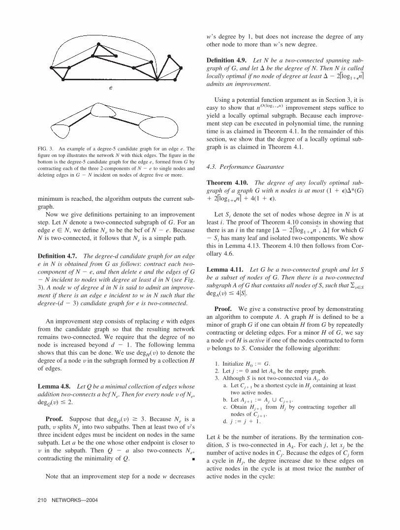
Next suppose that C has degree two or more in bcf(G Si2). Then C is internal to some path in bcf(G Si2)between leaf two-components L1 and L2. For j � 1, 2, letPj be the subpath from C to Lj. By Lemma 4.4, there is anedge ej of N between each Lj and Si2 for j � 1, 2. Wehave constructed edge-disjoint paths P1e1 and P2e2 from Cto A. The edges of these paths are in N � (G Si2) (seeFig. 4). Recall that A is two-connected and contains onlyedges in N, and that u is in A. It follows that C is two-connected to u using edges in (N � (G Si2) {e}).This contradicts the fact that the degree-(i 3) candidategraph for e is not two-connected. ■

Now we complete the proof of Lemma 4.13. The sum ofthe degrees of all the nodes of Si in N is at least i � �Si�. Bychoice of the set A, we have ¥v�Si2

degA(v) � 4(1� �)�Si�. Hence, there are at least �Si�(i 4(1 � �)) edgesincident on Si not in A. By Claim 4.15, each of these edgesgoes to a leaf two-component or isolated two-component ofbcf(G Si2). By the criticality of these edges in N, it alsofollows that there is at most one such edge to a leaf-component and at most two such edges to an isolated-component in bcf(G Si2). Hence, each such edgecontributes one to the deficiency of G Si2. This con-cludes the proof of Lemma 4.13. ■

5. DIRECTED MINIMUM-DEGREE SPANNINGTREE (DMDST) PROBLEM

5.1. Definitions and Notation

The input in this case is an arbitrary directed graph G� (V, E), and a root node r � V. Let n be the number of

FIG. 4. The edge (u, v) goes between u � Si2 and a node v in atwo-component C in the bcf of G Si2.

NETWORKS—2004 211

nodes in G. It is assumed that r is reachable from all nodesof G.

A branching rooted at r is a subgraph of G, whoseunderlying undirected graph is a spanning tree such that ithas a directed path from any node to r. In a branching, eachnode other than r has exactly one outgoing edge; r has nooutgoing edges. Sometimes this is also known as an in-branching. One can also define the notion of an out-branch-ing, in which r can reach every node of G through directedpaths. In this article, a branching always refers to an in-branching. Note that our algorithm can be easily modified tofind out-branchings of small outdegree.

Let T be a branching. For each edge (v, w) in T, we callw the parent of v, denoted by parent[v]. Because every nodeexcept r has a unique outgoing edge in T, each node has aunique parent, and r has none. The reflexive and transitiveclosure of the parent function yields the ancestor relation. Inother words, v is an ancestor of u if there is a directed pathin the branching from u to v. We call u a descendant of v ifv is its ancestor. We say that two nodes v and w are relatedif either v is an ancestor of w, or vice versa. Otherwise wesay that the nodes are unrelated. For any two unrelatednodes v and w, the least common ancestor is the ancestorclosest to v that is also an ancestor of w. We define Cv to bethe set of all nodes in the subtree rooted at v, i.e., the set ofall nodes including v, for which v is an ancestor.

The degree of a node in a given branching is the numberof edges coming into that node. We may also refer to this asthe indegree. For a branching, let S� be the set of all nodeswhose degree is � or more. The degree of a branching is themaximum degree of any of its nodes. Let T* be an optimalDMDST whose maximal degree is �*. Our goal is to find abranching whose (in)degree is as small as possible.

5.2. MDST Problem: Directed vs. Undirected Graphs

To extend the earlier algorithms to directed graphs, wehave to take note of the following differences.

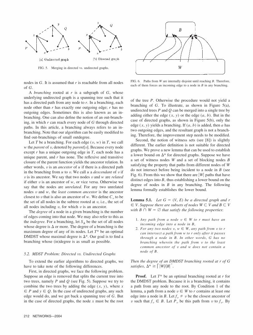
First, in directed graphs, we face the following problem.Suppose an edge is removed that splits the current tree intotwo trees, namely P and Q (see Fig. 5). Suppose we try tocombine the two trees by adding the edge ( x, y), where x� P and y � Q. In the case of undirected graphs, any suchedge would do, and we get back a spanning tree of G. Butin the case of directed graphs, the node x must be the root

of the tree P. Otherwise the procedure would not yield abranching of G. To illustrate, as shown in Figure 5(a),undirected trees P and Q can be merged into a single tree byadding either the edge ( x, y) or the edge (a, b). But in thecase of directed graphs, as shown in Figure 5(b), only theedge ( x, y) yields a branching. If (a, b) is added, then a hastwo outgoing edges, and the resultant graph is not a branch-ing. Therefore, the improvement step needs to be modified.

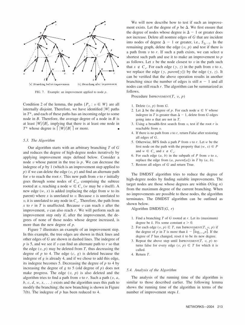
Second, the notion of witness sets (see [8]) is slightlydifferent. The earlier definition is not suitable for directedgraphs. We prove a new lemma that can be used to establisha lower bound on �* for directed graphs. Suppose we havea set of witness nodes W and a set of blocking nodes Bsatisfying the property that paths from different nodes of Wdo not intersect before being incident to a node in B (seeFig. 6). From this we show that there are �W� paths that havedistinct edges into B, thus establishing a lower bound on thedegree of nodes in B in any branching. The followinglemma formally establishes the lower bound.

Lemma 5.1. Let G � (V, E) be a directed graph and r� V. Suppose there are subsets of nodes W � V and B � Vwith B � W � A that satisfy the following properties:

1. Any path from a node v � W to r must have anincoming edge into a node in B,

2. For any two nodes v, w � W, any path from v to rcan intersect a path from w to r only after it passesthrough a node in B. In other words, G has nobranching wherein the path from v to the leastcommon ancestor of v and w does not contain anode of B.

Then the degree of an DMDST branching rooted at r of Gsatisfies, �* � �W�/�B� .

Proof. Let T* be an optimal branching rooted at r forthe DMDST problem. Because it is a branching, it containsa path from any node to the root. By Condition 1 of thelemma, a path from a node v � W to r contains at least oneedge into a node in B. Let fv v be the closest ancestor ofv such that fv � B. Let Pv be this path from v to fv. By

FIG. 5. Merging in directed vs. undirected graphs.

FIG. 6. Paths from W are internally disjoint until reaching B. Therefore,each of them forces an incoming edge to a node in B in any branching.

212 NETWORKS—2004

Condition 2 of the lemma, the paths {Pv : v � W} are allinternally disjoint. Therefore, we have identified �W� pathsin T*, and each of these paths has an incoming edge to somenode in B. Therefore, the average degree of a node in B isat least �W�/�B�, implying that there is at least one node inT* whose degree is �W�/�B� or more. ■

5.3. The Algorithm

Our algorithm starts with an arbitrary branching T of Gand reduces the degree of high-degree nodes iteratively byapplying improvement steps defined below. Consider anode v whose parent in the tree is p. We can decrease theindegree of p by 1 (which is an improvement step applied top) if we can delete the edge (v, p) and find an alternate pathfor v to reach the root r. This new path from v to r initiallygoes through some nodes of Cv, comprising the subtreerooted at v, reaching a node w � Cv (w may be v itself). Anew edge (w, x) is added (replacing the edge from w to itsparent) where x is unrelated to v. Because x is unrelated tov, it is unrelated to any node in Cv. Therefore, the path fromx to r in T is unaffected. Because v can reach x after theimprovement, v can also reach r. We will perform such animprovement step only if, after the improvement, the de-grees of none of those nodes whose degree increased, ismore than the new degree of p.

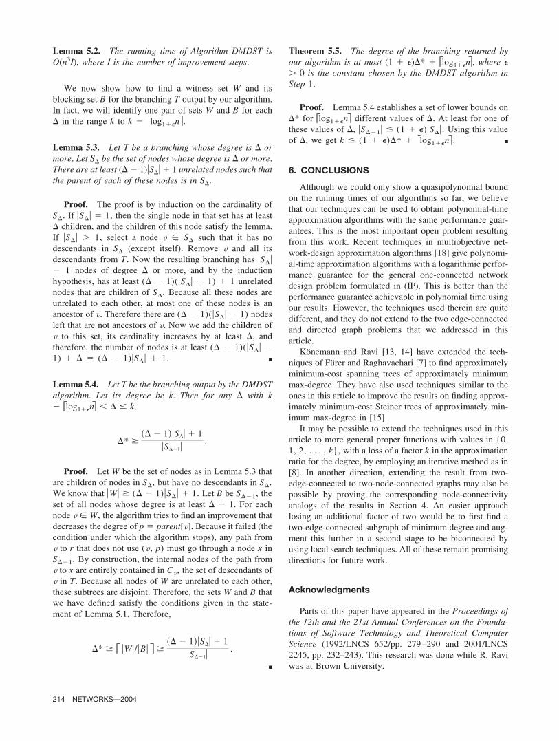
Figure 7 illustrates an example of an improvement step.In this example, the tree edges are shown in thick lines andother edges of G are shown in dashed lines. The indegree ofp is 5, and we see if v can find an alternate path to r so thatthe edge (v, p) may be deleted from T, thus decreasing thedegree of p to 4. The edge (c, g) is deleted because theindegree of g is already 4, and if we chose to add this edge,its indegree becomes 5. Decreasing the degree of p to 4 byincreasing the degree of g to 5 (old degree of p) does notmake progress. The edge (v, p) is also deleted and thealgorithm tries to find a path from v to r. Such a path (v, a,b, c, d, w, x, . . .) exists and the algorithm uses this path tomodify the branching; the new branching is shown in Figure7(b). The indegree of p has been reduced to 4.

We will now describe how to test if such an improve-ment exists. Let the degree of p be �. We first ensure thatthe degree of nodes whose degree is � 1 or greater doesnot increase. Delete all nontree edges of G that are incidentinto nodes of degree � 1 or greater, i.e., S�1. In theremaining graph, delete the edge (v, p) and test if there isa path from v to r. If such a path exists, we can select ashortest such path and use it to make an improvement to pas follows. Let x be the node closest to v in the path suchthat x � Cv. For each edge ( y, z) in the path from v to x,we replace the edge ( y, parent[ y]) by the edge ( y, z). Itcan be verified that the above operation results in anotherbranching since the number of edges is still n 1 and allnodes can still reach r. The algorithm can be summarized asfollows.

Procedure IMPROVEMENT(T, v, p)

1. Delete (v, p) from G.2. Let � be the degree of p. For each node u � V whose

indegree in T is greater than � 1, delete from G edgesgoing into u that are not in T.

3. Using a breadth-first search from v, test if the root r isreachable from v.

4. If there is no path from v to r, return False after restoringall edges of G.

5. Otherwise, BFS finds a path P from v to r. Let w be thefirst node on the path with the property that (w, x) � Pand w � Cv and x � Cv.

6. For each edge (a, b) in the subpath of P from v to x,replace the edge from (a, parent[a]) in T by (a, b).

7. Restore all edges of G and return True.

The DMDST algorithm tries to reduce the degree ofhigh-degree nodes by finding suitable improvements. Thetarget nodes are those whose degrees are within O(log n)from the maximum degree of the current branching. Whenno improvements are possible to these nodes, the algorithmterminates. The DMDST algorithm can be outlined asshown below.

Algorithm DMDST(G, r)

1. Find a branching T of G rooted at r. Let its (maximum)degree be k. Fix some constant � � 0.

2. For each edge (v, p) � T, run IMPROVEMENT(T, v, p) ifthe degree of p in T is more than k log1��n . If thedegree of T has changed, reset k to be its new degree.

3. Repeat the above step until IMPROVEMENT(T, v, p) re-turns false for every edge (v, p) � T for which it iscalled.

4. Return T.

5.4. Analysis of the Algorithm

The analysis of the running time of the algorithm issimilar to those described earlier. The following lemmashows the running time of the algorithm in terms of thenumber of improvement steps I.

FIG. 7. Example: an improvement applied to node p.

NETWORKS—2004 213

Lemma 5.2. The running time of Algorithm DMDST isO(n3I), where I is the number of improvement steps.

We now show how to find a witness set W and itsblocking set B for the branching T output by our algorithm.In fact, we will identify one pair of sets W and B for each� in the range k to k log1��n .

Lemma 5.3. Let T be a branching whose degree is � ormore. Let S� be the set of nodes whose degree is � or more.There are at least (� 1)�S�� � 1 unrelated nodes such thatthe parent of each of these nodes is in S�.

Proof. The proof is by induction on the cardinality ofS�. If �S�� � 1, then the single node in that set has at least� children, and the children of this node satisfy the lemma.If �S�� � 1, select a node v � S� such that it has nodescendants in S� (except itself). Remove v and all itsdescendants from T. Now the resulting branching has �S�� 1 nodes of degree � or more, and by the inductionhypothesis, has at least (� 1)(�S�� 1) � 1 unrelatednodes that are children of S�. Because all these nodes areunrelated to each other, at most one of these nodes is anancestor of v. Therefore there are (� 1)(�S�� 1) nodesleft that are not ancestors of v. Now we add the children ofv to this set, its cardinality increases by at least �, andtherefore, the number of nodes is at least (� 1)(�S�� 1) � � � (� 1)�S�� � 1. ■

Lemma 5.4. Let T be the branching output by the DMDSTalgorithm. Let its degree be k. Then for any � with k log1��n � � � k,

�* ��� � 1��S�� 1

�S�1�.

Proof. Let W be the set of nodes as in Lemma 5.3 thatare children of nodes in S�, but have no descendants in S�.We know that �W� � (� 1)�S�� � 1. Let B be S�1, theset of all nodes whose degree is at least � 1. For eachnode v � W, the algorithm tries to find an improvement thatdecreases the degree of p � parent[v]. Because it failed (thecondition under which the algorithm stops), any path fromv to r that does not use (v, p) must go through a node x inS�1. By construction, the internal nodes of the path fromv to x are entirely contained in Cv, the set of descendants ofv in T. Because all nodes of W are unrelated to each other,these subtrees are disjoint. Therefore, the sets W and B thatwe have defined satisfy the conditions given in the state-ment of Lemma 5.1. Therefore,

�* � �W�/�B� ��� � 1��S�� 1

�S�1�.

■

Theorem 5.5. The degree of the branching returned byour algorithm is at most (1 � �)�* � log1��n , where �� 0 is the constant chosen by the DMDST algorithm inStep 1.

Proof. Lemma 5.4 establishes a set of lower bounds on�* for log1��n different values of �. At least for one ofthese values of �, �S�1� � (1 � �)�S��. Using this valueof �, we get k � (1 � �)�* � log1��n . ■

6. CONCLUSIONS

Although we could only show a quasipolynomial boundon the running times of our algorithms so far, we believethat our techniques can be used to obtain polynomial-timeapproximation algorithms with the same performance guar-antees. This is the most important open problem resultingfrom this work. Recent techniques in multiobjective net-work-design approximation algorithms [18] give polynomi-al-time approximation algorithms with a logarithmic perfor-mance guarantee for the general one-connected networkdesign problem formulated in (IP). This is better than theperformance guarantee achievable in polynomial time usingour results. However, the techniques used therein are quitedifferent, and they do not extend to the two edge-connectedand directed graph problems that we addressed in thisarticle.

Konemann and Ravi [13, 14] have extended the tech-niques of Furer and Raghavachari [7] to find approximatelyminimum-cost spanning trees of approximately minimummax-degree. They have also used techniques similar to theones in this article to improve the results on finding approx-imately minimum-cost Steiner trees of approximately min-imum max-degree in [15].

It may be possible to extend the techniques used in thisarticle to more general proper functions with values in {0,1, 2, . . . , k}, with a loss of a factor k in the approximationratio for the degree, by employing an iterative method as in[8]. In another direction, extending the result from two-edge-connected to two-node-connected graphs may also bepossible by proving the corresponding node-connectivityanalogs of the results in Section 4. An easier approachlosing an additional factor of two would be to first find atwo-edge-connected subgraph of minimum degree and aug-ment this further in a second stage to be biconnected byusing local search techniques. All of these remain promisingdirections for future work.

Acknowledgments

Parts of this paper have appeared in the Proceedings ofthe 12th and the 21st Annual Conferences on the Founda-tions of Software Technology and Theoretical ComputerScience (1992/LNCS 652/pp. 279–290 and 2001/LNCS2245, pp. 232–243). This research was done while R. Raviwas at Brown University.

214 NETWORKS—2004

REFERENCES

[1] A. Agrawal, P. Klein, and R. Ravi, How tough is theminimum-degree Steiner tree? An approximate min–maxequality (complete with algorithms), Tech Rep-CS-91-49,Brown University, 1991.

[2] A. Agrawal, P. Klein, and R. Ravi, When trees collide: Anapproximation algorithm for the generalized Steiner treeproblem on networks, SIAM J Comput 24 (1995), 445–456.

[3] D. Bauer, S.L. Hakimi, and E. Schmeichel, Recognizingtough graphs is NP-hard, Discrete Appl Math 28 (1990),191–195.

[4] V. Chvatal, Tough graphs and Hamiltonian circuits, Dis-crete Math 5 (1973), 215–228.

[5] M. Furer and B. Raghavachari, An �� approximation al-gorithm for the minimum-degree spanning tree problem,Proc 28th Ann Allerton Conference on Communication,Control and Computing, Monticello, IL, 1990, pp. 274–281.

[6] M. Furer and B. Raghavachari, Approximating the mini-mum-degree spanning tree to within one from the optimaldegree, Proc 3rd Ann ACM-SIAM Symp Discrete Algo-rithms, Orlando, FL, 1992, pp. 317–324.

[7] M. Furer and B. Raghavachari, Approximating the mini-mum-degree Steiner tree to within one of optimal, J Algo-rithms 17 (1994), 409–423.

[8] H.N. Gabow, M.X. Goemans, and D.P. Williamson, Anefficient approximation algorithm for the survivable net-work design problem, Math Program 82 (1998), 13–40.

[9] M.R. Garey and D.S. Johnson, Computers and intractability:A guide to the theory of NP-completeness, W.H. Freeman,San Francisco, 1979.

[10] B. Gavish, Topological design of centralized computer net-works—Formulations and algorithms, Networks 12 (1982),355–377.

[11] M.X. Goemans and D.P. Williamson, A general approxi-mation technique for constrained forest problems, SIAMJ Comput 24 (1995), 296–317.

[12] M. Grotschel, L. Lovasz, and A. Schrijver, Geometric al-gorithms and combinatorial optimization, Springer-Verlag,Berlin, 1988.

[13] J. Konemann and R. Ravi, A matter of degree: Improvedapproximation algorithms for degree-bounded minimumspanning trees, SIAM J Comput 31 (2002), 1783–1793.

[14] J. Konemann and R. Ravi, Primal-dual meets local search:Approximating MST’s with nonuniform degree bounds,Proc 35th Ann Symp Theory Comput ACM, San Diego,CA, 2003, pp. 389–395.

[15] J. Konemann and R. Ravi, Quasi-polynomial time approx-imation algorithm for low-degree minimum-cost Steinertrees, Proc 23rd Conf Foundations of Software Technologyand Theoretical Computer Science, Mumbai, India, LectureNotes in Computer Science 2914, Springer 2003, pp. 289–301.

[16] E.L. Lawler, Combinatorial optimization: Networks andmatroids, Holt, Rinehart and Winston, New York, 1976.

[17] G.L. Nemhauser and L.A. Wolsey, Integer and combinato-rial optimization, Wiley, New York, 1988.

[18] R. Ravi, M.V. Marathe, S.S. Ravi, D.J. Rosenkrantz, andH.B. Hunt, III, Approximation algorithms for degree-con-strained minimum-cost network-design problems, Algorith-mica 31 (2001), 58–78.

[19] D.P. Williamson, M.X. Goemans, M. Mihail, and V.Vazirani, A primal-dual approximation algorithm for gen-eralized Steiner network problems, Combinatorica 15(1995), 435–454.

[20] S. Win, On a connection between the existence of k-treesand the toughness of a graph, Graphs Combinatorics 5(1989), 201–205.

NETWORKS—2004 215