Approximation algorithms for hierarchical location problems

Journal of Computer and System Sciences 72 (2006) 425–443www.elsevier.com/locate/jcss

Approximation algorithms for hierarchical location problems�

C. Greg Plaxton

Department of Computer Science, University of Texas at Austin, Austin, TX 78712–1188, USA

Received 7 November 2003; received in revised form 25 February 2005

Available online 7 November 2005

Abstract

We formulate and (approximately) solve hierarchical versions of two prototypical problems in discrete locationtheory, namely, the metric uncapacitated k-median and facility location problems. Our work yields new insightsinto hierarchical clustering, a widely used technique in data analysis. For example, we show that every metric spaceadmits a hierarchical clustering that is within a constant factor of optimal at every level of granularity with respectto the average (squared) distance objective. A key building block of our hierarchical facility location algorithm isa constant-factor approximation algorithm for an “incremental” variant of the facility location problem; the latteralgorithm may be of independent interest.© 2005 Elsevier Inc. All rights reserved.

Keywords: Discrete location theory; Hierarchical clustering

1. Introduction

In independent recent work, Charikar et al. [3] and Dasgupta and Long [6] formulated and solved anatural hierarchical version of the k-center problem. In this paper, we extend this line of research byinvestigating hierarchical versions of the metric uncapacitated k-median and facility location problems,two prototypical problems in discrete location theory. Before introducing the hierarchical versions ofthese problems, we review the definitions of the k-center, k-median, and facility location problems.We also review certain “incremental” versions of the k-center and k-median problems, and introduce a

�This material is based upon work supported by the National Science Foundation under Grant Nos. 9821053 and 0310970.The author is also affiliated with Akamai Technologies, Inc., Cambridge, MA 02142, USA.

URL:http://www.cs.utexas.edu/users/plaxton.

0022-0000/$ - see front matter © 2005 Elsevier Inc. All rights reserved.doi:10.1016/j.jcss.2005.09.004

http://www.elsevier.com/locate/jcss

http://www.cs.utexas.edu/users/plaxton

426 C. Greg Plaxton / Journal of Computer and System Sciences 72 (2006) 425–443

corresponding incremental version of the facility location problem. The incremental versions of theseproblems represent a natural intermediate step towards defining their hierarchical versions.

1.1. Preliminaries

For any real � � 1, we say that a distance function d defined over a set of points satisfies the �-approximate triangle inequality if, for any triple of points x, y, and z, d(x, z) � �(d(x, y)+d(y, z)). Wedefine an �-approximate metric space as a set of points with an associated distance function d that satisfiespositivity (d(x, y) > 0 unless x = y, in which case d(x, y) = 0), symmetry (d(x, y) = d(y, x)), and the�-approximate triangle inequality. Our motivation for assuming such a relaxed triangle inequality is thatsquaring each of the distances in a given metric space yields a 2-approximate metric space. More generally,raising the distances of a metric space to any constant power yields an �-approximate metric space for someconstant � � 1. Consequently, the various constant-factor approximation algorithms that we develop inthis paper for �-approximate metric spaces immediately imply constant-factor approximation algorithmsfor related problems on metric spaces in which the objective function is altered by raising each distanceto some constant power. In keeping with the foregoing motivation, we will assume throughout the paperthat the parameter � governing the relaxed triangle inequality is a constant. In our discussions of priorwork, we generally restrict our attention to the important special case � = 1, since most of the existingwork assumes a strict triangle inequality.

In this paper, we will define approximation versions of various optimization problems. As a convenientshorthand, throughout this paper we define an approximation algorithm for a given problem to be nice ifand only if it is constant-factor approximate and runs in polynomial time. Remark: The constant factor inthe approximation bound is allowed to depend on the constant � governing the relaxed triangle inequality.

Throughout the remainder of the paper, we fix an arbitrary �-approximate metric space with associatednonempty point set U and distance function d. We let n denote |U |, we define an index as an integerin the range 1–n inclusive, and we define a scaling factor as a nonnegative real. Each point x has anassociated nonnegative weight w(x) and value v(x). For any set of points X, we let w(X) = ∑

x∈X w(x)

and v(X) = ∑x∈X v(x). As a minor technical convenience, we assume that w(U) > 0, i.e., that at least

one point in U has positive weight. (The problems we intend to address are not interesting when all ofthe weights are zero.)

For any point x, nonempty sets of points X and Y , and scaling factor �, we define

d(x, Y ) = miny∈Y

d(x, y), (1)

radius(X, Y ) = maxx∈X

d(x, Y ), (2)

error(X, Y ) =∑x∈X

d(x, Y ) · w(x), (3)

cost�(X, Y ) = � · error(X, Y ) + v(Y ). (4)

Remark: We occasionally abuse our notation slightly by identifying a singleton set with its lone element.For example, we generally write error(X, x) instead of error(X, {x}).

For any nonempty set of points X and integer k, 1 � k � |X|, we let radiusk(X) (resp., errork(X))denote the minimum, over all subsets Y of X such that |Y | = k, of radius(X, Y ) (resp., error(X, Y )).

C. Greg Plaxton / Journal of Computer and System Sciences 72 (2006) 425–443 427

Similarly, for any scaling factor � and nonempty set of points X, we let cost�(X) denote the minimum,over all nonempty subsets Y of X, of cost�(X, Y ).

1.2. The k-center and k-median problems

A nonempty set of points X is said to achieve a radius (resp., error) ratio of a if radius(U, X) (resp.,error(U, X)) is at most a times radius|X|(U) (resp., error|X|(U)). Given an index k, the k-center (resp.,k-median) problem asks us to determine a set of k points with minimum radius (resp., error). A k-center(resp., k-median) algorithm is a-approximate if it computes a set of k points with radius (resp, error)ratio a.

We now give a brief overview of the approximability results known for the k-center and k-medianproblems. The farthest point technique of Gonzalez [9] yields a simple 2-approximate k-center algorithmrunning in O(nk) time. This factor-of-2 bound is matched by Hochbaum and Shmoys [11] (albeit witha somewhat worse running time) using a more general approximation technique that is applicable to acertain class of “bottleneck” problems that includes k-center. Hochbaum and Shmoys [11] also show thatno polynomial time k-center algorithm can achieve an approximation factor better than 2 unless P = NP.Thus, the approximability of k-center is well understood. The situation with respect to the k-medianproblem is somewhat more complicated. The first nice k-median algorithm is due to Charikar et al. [4].That result has subsequently been improved in terms of both quality of approximation and running time.Currently, the best approximation factor associated with any nice k-median algorithm is 3 + ε, where ε

is an arbitrarily small positive constant; this result is due to Arya et al. [1]. Jain et al. [12] show that thereis no nice (1 + 2/e)-approximate k-median algorithm unless NP ⊆ DTIME[nO(log log n)]. The reader isreferred to [12] for a more complete survey of prior work on the k-median problem.

1.3. The incremental center and median problems

We define a rank function as a numbering of the points from 0 to n − 1. A rank function r is saidto achieve a radius (resp., error) ratio of a if for any index k, radius(U, {x ∈ U | r(x) < k) (resp.,error(U, {x ∈ U | r(x) < k)), is at most a times radiusk(U) (resp., errork(U)). The incremental center(resp., median) problem asks us to determine a rank function r with minimum radius (resp., error) ratio.An incremental center (resp., median) algorithm is a-approximate if it computes a rank function withradius (resp., error) ratio a.

The farthest point technique of Gonzalez [9] provides a 2-approximate O(n2)-time incremental centeralgorithm. The hardness result for the k-center problem implies that no polynomial time incrementalcenter algorithm can achieve a better radius ratio unless P = NP. The incremental median problem isaddressed in [14], where it is motivated within an online framework and referred to as the online medianproblem. The incremental k-median algorithm of Mettu and Plaxton [14] runs in O(n2) time if the ratioof the maximum interpoint distance to the minimum interpoint distance is 2O(n), and achieves a cost ratioof approximately 30. More recently, Mettu and Plaxton [15] have presented the fastest (randomized) nicek-median algorithm known. That algorithm runs in O(nk) time for k between log n and n

log2 n; see [15]

for the general time bound.


1.4. The facility location problem

We say that a nonempty set of points X has a cost ratio of a with respect to a given scaling factor � ifcost�(U, X) � a · cost�(U). The facility location problem asks us to determine a nonempty set of pointswith minimum cost with respect to a given scaling factor. A facility location algorithm is a-approximateif it computes a set of points with cost ratio a with respect to any given scaling factor.

The first nice facility location algorithm is due to Shmoys et al. [17]. That algorithm has subsequentlybeen improved, both in terms quality of approximation and running time. Currently, the best approximationbound established for any nice facility location algorithm is approximately 1.52; this result is due toMahdian et al. [13]. Guha and Kuller [10] show that there is no nice 1.463-approximate facility locationalgorithm unless NP ⊆ DTIME[nO(log log n)]. The fastest nice facility location algorithm known is theO(n2)-time greedy algorithm presented in [14], which achieves an approximation ratio of 3. Anothernoteworthy result is Thorup’s recent O(n+m)-time 1.62-approximate facility location algorithm for thecase in which the input metric space is the shortest path metric of a weighted undirected graph with nnodes and m edges. (Here the O notation suppresses logarithmic factors.) The reader is referred to [13,18]for a more complete survey of prior work on the facility location problem.

1.5. The incremental facility location problem

In this section, we introduce a new variant of the facility location problem that we call the incrementalfacility location problem. Our goal is to formulate a facility location analogue of the incremental medianproblem discussed earlier. In the incremental median problem, the objective is to construct a sequence ofnear-optimal k-median solutions, 1 � k � n, such that no point is ever removed from our solution as k

increases. Note that the facility location parameter � plays a qualitatively similar role as the parameter k inthe k-median problem: for small values of �, a good solution can be expected to contain a small number offacilities, and for large values of �, a good solution can be expected to contain a large number of facilities.This observation motivates us to ask whether there exists a rank function and a nondecreasing functionf from the set of scaling factors to the set of indices such that for any scaling factor �, if f (�) = k, thenthe set of k points with ranks less than k form a near-optimal solution to the facility location problem.Given the foregoing motivation, we now develop a formal definition of the incremental facility locationproblem.

A threshold sequence is a nondecreasing sequence of values 0 = t1 � t2 � · · · � tn drawn fromR ∪ {∞}.

We say that a rank function r and threshold sequence 0 = t1 � t2 � · · · � tn achieve a cost ratio of a

if for any scaling factor �,

cost�(U, {x ∈ U | r(x) < k}) � a · cost�(U), (5)

where k is the largest index such that tk � �.The incremental facility location problem asks us to determine a rank function and threshold sequence

with minimum cost ratio. An incremental facility location algorithm is said to be a-approximate if it com-putes a rank function and threshold sequence with cost ratio a. There is no prior work on the incrementalfacility location problem as we are introducing it in the present paper.


1.6. Hierarchical clustering

Hierarchical clustering is a longstanding and widely used technique in data analysis. It is described,for example, in the classic 1973 pattern classification text of Duda and Hart [7]. (See also therecent second edition of this text [8].) In this subsection, we review the definition of a hierarchicalclustering and describe the classic dendrogram-based approach to depicting a given a hierarchicalclustering.

A clustering is a partition of U into a number of nonempty sets, or clusters.A k-clustering is a clusteringwith k clusters. The radius (resp., error) of a k-clustering with associated clusters Xi , 0 � i < k, is definedas max0 � i < k radius1(Xi) (resp.,

∑0 � i < k error1(Xi)).

A hierarchical clustering is a set of n clusterings containing one k-clustering for each index k, andsuch that for any index k less than n, the (k + 1)-clustering can be transformed into the k-clustering bymerging some pair of clusters.

Question 1. Does every metric space admit a hierarchical clustering for which each associated k-clustering has radius (resp., error) within a constant factor of optimal?

Charikar et al. [3] and Dasgupta and Long [6] independently answered the radius version of Question 1in the affirmative. But their work leaves open the question of whether a similar result holds with respectto error. In Section 1.8, we define the notion of a hierarchical ordering and formulate a stronger versionof Question 1 with respect to hierarchical orderings.

The aforementioned hierarchical clustering algorithm of Charikar et al. may also be viewed as a k-center algorithm that allows the solution to be easily updated when a point is added to the metric space.In fact, their algorithm only needs to “remember” the k points of the current solution as the input metricspace grows; see [3] for a precise statement of the upper bound model. Charikar and Panigrahy [5, Section7.3] prove that for the strictest version of the upper bound model it is not possible to obtain an analogousconstant-factor approximation algorithm with respect to the error objective, that is, for the k-medianproblem. (We caution the reader that the term “incremental” is used differently in the present paper thanin [3,5]; here it refers to incrementing the parameter k as opposed to incrementing the size of the probleminstance.)

We remark that there are∏

2�k�n

(k2

) = n!(n − 1)!21−n distinct hierarchical clusterings of U , since

there is a unique n-clustering and there are(k2

)different merge operations that can be applied to any

k-clustering to obtain a (k − 1)-clustering. Furthermore, the sequence of n − 1 merges performed insuccessively transforming the n-clustering into the 1-clustering induce an n-leaf binary tree in whicheach leaf corresponds to a point and each of the n − 1 internal nodes corresponds to a merge. Thus,it is natural to consider depicting a hierarchical clustering using a standard binary tree diagram. Theshortcoming of such a representation is that information regarding the relative order of the merges is, ingeneral, lost. For example, in a binary tree in which several nodes appear at the same level, we cannottell in which order the corresponding merges are performed.

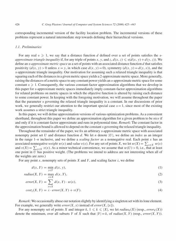
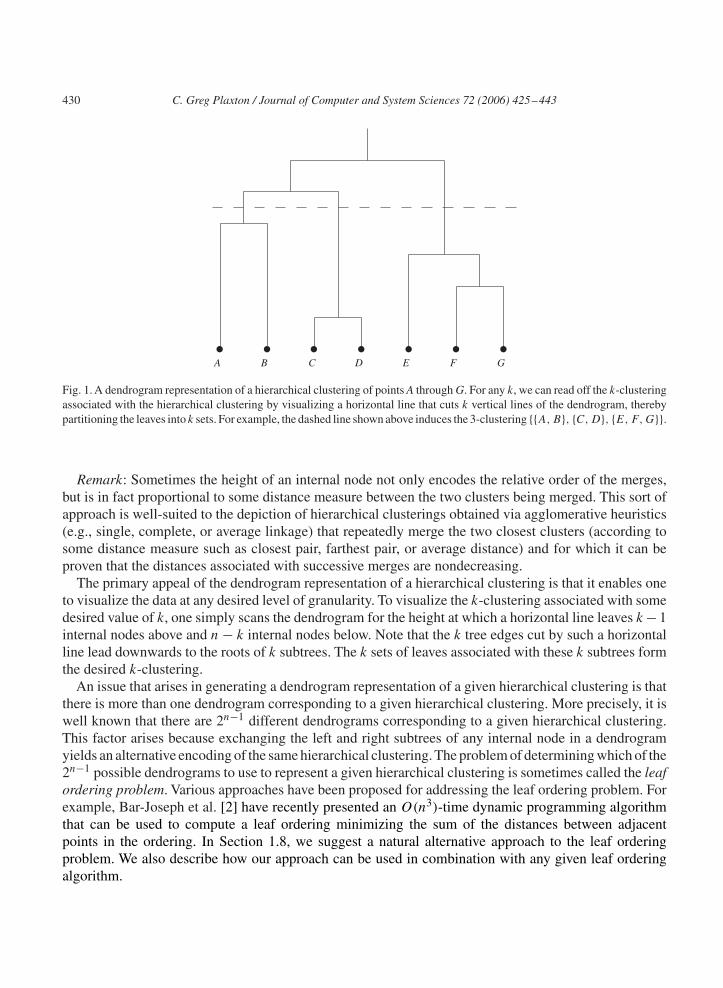
A dendrogram is a drawing of a binary tree that preserves the total order on the internal nodes (inducedby the merge operations) by ensuring that no two internal nodes appear at the same height on the page. Inaddition, the n leaves are normally arranged along a horizontal line at the bottom of the tree. See Fig. 1for an example of a dendrogram.


A B C D E F G

Fig. 1. A dendrogram representation of a hierarchical clustering of points A through G. For any k, we can read off the k-clusteringassociated with the hierarchical clustering by visualizing a horizontal line that cuts k vertical lines of the dendrogram, therebypartitioning the leaves into k sets. For example, the dashed line shown above induces the 3-clustering {{A, B}, {C, D}, {E, F, G}}.

Remark: Sometimes the height of an internal node not only encodes the relative order of the merges,but is in fact proportional to some distance measure between the two clusters being merged. This sort ofapproach is well-suited to the depiction of hierarchical clusterings obtained via agglomerative heuristics(e.g., single, complete, or average linkage) that repeatedly merge the two closest clusters (according tosome distance measure such as closest pair, farthest pair, or average distance) and for which it can beproven that the distances associated with successive merges are nondecreasing.

The primary appeal of the dendrogram representation of a hierarchical clustering is that it enables oneto visualize the data at any desired level of granularity. To visualize the k-clustering associated with somedesired value of k, one simply scans the dendrogram for the height at which a horizontal line leaves k − 1internal nodes above and n − k internal nodes below. Note that the k tree edges cut by such a horizontalline lead downwards to the roots of k subtrees. The k sets of leaves associated with these k subtrees formthe desired k-clustering.

An issue that arises in generating a dendrogram representation of a given hierarchical clustering is thatthere is more than one dendrogram corresponding to a given hierarchical clustering. More precisely, it iswell known that there are 2n−1 different dendrograms corresponding to a given hierarchical clustering.This factor arises because exchanging the left and right subtrees of any internal node in a dendrogramyields an alternative encoding of the same hierarchical clustering. The problem of determining which of the2n−1 possible dendrograms to use to represent a given hierarchical clustering is sometimes called the leafordering problem. Various approaches have been proposed for addressing the leaf ordering problem. Forexample, Bar-Joseph et al. [2] have recently presented an O(n3)-time dynamic programming algorithmthat can be used to compute a leaf ordering minimizing the sum of the distances between adjacentpoints in the ordering. In Section 1.8, we suggest a natural alternative approach to the leaf orderingproblem. We also describe how our approach can be used in combination with any given leaf orderingalgorithm.


1.7. Hierarchical assignment

In this section, we introduce a variant of the notion of a hierarchical clustering that we refer to as ahierarchical assignment.

An assignment is a function from U to U . A k-assignment is an assignment with a range of size k.The radius (resp., error) of an assignment � is defined as maxx∈U d(x, �(x)) (resp.,

∑x∈U d(x, �(x))

· w(x)).A hierarchical assignment is a set of n assignments containing one k-assignment for each index k, and

such that for any index k less than n, there exists a pair of points x and y for which the (k+1)-assignmentcan be transformed into the k-assignment by reassigning to x all points assigned to y. Note that thistransformation may be viewed as an “oriented merge” of the two sets of points mapped to x and y in the(k + 1)-assignment. (We consider the merge to be oriented because the union of these sets of points isassigned to x, and not y, in the k-assignment.)

A notable difference between a hierarchical assignment and a hierarchical clustering is that while thereis only one n-clustering of U , there are n! possible n-assignments, one corresponding to each permutation.Furthermore, for k > 1, there are k(k − 1) different oriented merge operations that can be applied to anyk-assignment to obtain a (k − 1)-assignment. It follows that there are exactly (n!)2(n − 1)! distincthierarchical assignments of U .

We define a parent function p with respect to a given rank function r as a mapping from U to U suchthat p(x) = x if r(x) = 0 and r(p(x)) < r(x) otherwise.

The above discussion suggests the following permutation-rank-parent representation in which a hierar-chical assignment with associated k-assignment �k , 1 � k � n is represented by specifying the followinginformation: (1) The permutation �n; (2) The rank function r such that the range of �k is equal to{x | r(x) < k}; (3) The parent function p with respect to r such that for any index k less than n, theoriented merge operation transforming �k+1 into �k reassigns to p(x) all points assigned to x, wherer(x) = k.

Note that there are n! choices for the permutation �n and n! choices for the rank function r . Furthermore,for every choice of �n and r , there are (n − 1)! choices for the parent function p. Thus there are (n!)2

(n − 1)! possible permutation-rank-parent representations, one for each hierarchical assignment.

1.8. Hierarchical ordering

We define a hierarchical ordering as a hierarchical assignment for which the associated k-assignmentis idempotent for all k. Note that the identity assignment is the only idempotent n-assignment on a setof n points. Furthermore, for any index k < n, if the (k + 1)-assignment associated with a hierarchicalassignment is idempotent, then so is the k-assignment. Thus, we can equivalently define a hierarchicalordering as a hierarchical assignment for which the associated n-assignment is the identity assignment.Thus the permutation-rank-parent representation for hierarchical assignments described in Section 1.7corresponds to a rank-parent representation for hierarchical orderings, and there are exactly n!(n − 1)!hierarchical orderings.

Question 2. Does every metric space admit a hierarchical ordering for which each associated k-assignment has radius (resp., error) within a constant factor of optimal?


The following view of a hierarchical ordering may be useful in order to better understand the relationshipbetween Question 2 above and Question 1. A hierarchical ordering may be interpreted as a hierarchicalclustering in which the points of each cluster are assigned to a unique “representative” point in the cluster,subject to the additional constraint that when two clusters X and Y are merged, the representative of theresulting cluster is required to be chosen as either the representative of X or the representative of Y . Ifwe were to drop the latter constraint, there would be no difference between the hierarchical orderingquestions posed above and the corresponding hierarchical clustering questions. But by constraining thechoice of representative, we only make it more difficult to remain within a constant factor of optimal forall indices k.

For the radius version of the problem, the �-approximate triangle inequality implies that for any clusterX and point x in X, radius(X, x) � 2� · radius1(X). Given that we are assuming � to be a constant, thisimplies that a given metric space admits a hierarchical ordering for which each associated k-assignmenthas radius within a constant factor of optimal if and only if it admits a hierarchical clustering for whicheach associated k-clustering has radius within a constant factor of optimal. So, the hierarchical clusteringalgorithms of Charikar et al. [3] and Dasgupta and Long [6] immediately provide a positive answer tothe radius version of Question 2.

For the error version of the problem, which is the primary focus of the present paper, note that the(weighted) sum of distances to the representative of a given cluster can vary dramatically (by a factoressentially as large as the diameter of the metric space) depending on the choice of cluster representative.Thus the error version of Question 2 is stronger than the error version of Question 1 in that a positiveanswer to the former question immediately implies a positive answer to the latter question, but not viceversa.

In Section 4 we resolve the error version of Question 2 in the affirmative, thereby also providing apositive answer to the error version of Question 1. (In fact, for any constant �, we provide a positiveanswer to Question 2 for any �-approximate metric space.)

Let us now briefly return to the leaf ordering problem mentioned at the end of Section 1.6. Earlier wesaw that the leaf ordering problem arises because there are 2n−1 different dendrograms corresponding to agiven hierarchical clustering. But the number of dendrograms is exactly equal to the number of hierarchicalorderings, so if we encode a hierarchical ordering as a dendrogram by adopting the convention that theleftmost leaf in each subtree is the representative of the cluster corresponding to that subtree, then theleaf ordering problem goes away.

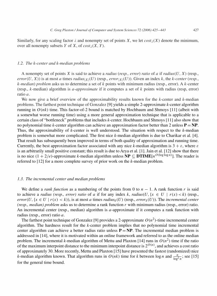
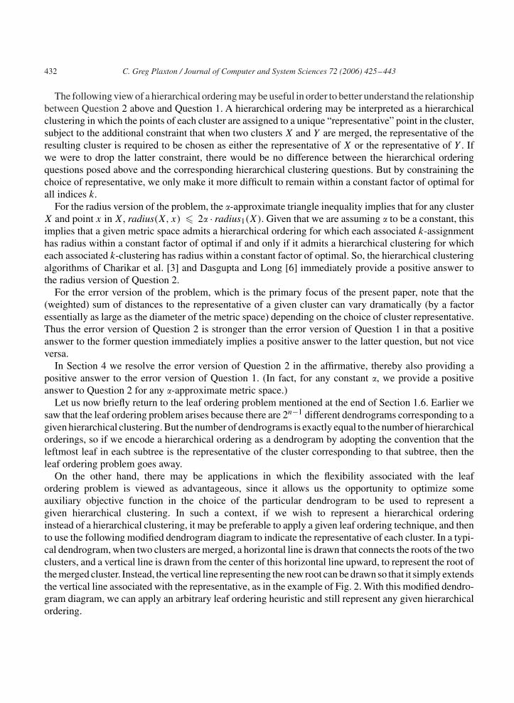
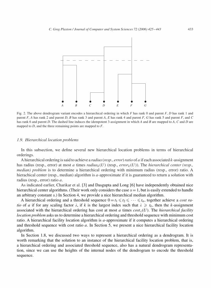
On the other hand, there may be applications in which the flexibility associated with the leafordering problem is viewed as advantageous, since it allows us the opportunity to optimize someauxiliary objective function in the choice of the particular dendrogram to be used to represent agiven hierarchical clustering. In such a context, if we wish to represent a hierarchical orderinginstead of a hierarchical clustering, it may be preferable to apply a given leaf ordering technique, and thento use the following modified dendrogram diagram to indicate the representative of each cluster. In a typi-cal dendrogram, when two clusters are merged, a horizontal line is drawn that connects the roots of the twoclusters, and a vertical line is drawn from the center of this horizontal line upward, to represent the root ofthe merged cluster. Instead, the vertical line representing the new root can be drawn so that it simply extendsthe vertical line associated with the representative, as in the example of Fig. 2. With this modified dendro-gram diagram, we can apply an arbitrary leaf ordering heuristic and still represent any given hierarchicalordering.


A B C D E F G

Fig. 2. The above dendrogram variant encodes a hierarchical ordering in which F has rank 0 and parent F, D has rank 1 andparent F, A has rank 2 and parent D, B has rank 3 and parent A, E has rank 4 and parent F, G has rank 5 and parent F, and Chas rank 6 and parent D. The dashed line induces the idempotent 3-assignment in which A and B are mapped to A, C and D aremapped to D, and the three remaining points are mapped to F.

1.9. Hierarchical location problems

In this subsection, we define several new hierarchical location problems in terms of hierarchicalorderings.

A hierarchical ordering is said to achieve a radius (resp., error) ratio of a if each associated k-assignmenthas radius (resp., error) at most a times radiusk(U) (resp., errork(U)). The hierarchical center (resp.,median) problem is to determine a hierarchical ordering with minimum radius (resp., error) ratio. Ahierachical center (resp., median) algorithm is a-approximate if it is guaranteed to return a solution withradius (resp., error) ratio a.

As indicated earlier, Charikar et al. [3] and Dasgupta and Long [6] have independently obtained nicehierarchical center algorithms. (Their work only considers the case � = 1, but is easily extended to handlean arbitrary constant �.) In Section 4, we provide a nice hierarchical median algorithm.

A hierarchical ordering and a threshold sequence 0 = t1 � t2 � · · · � tn, together achieve a cost ra-tio of a if for any scaling factor �, if k is the largest index such that � � tk , then the k-assignmentassociated with the hierarchical ordering has cost at most a times cost�(U). The hierarchical facilitylocation problem asks us to determine a hierarchical ordering and threshold sequence with minimum costratio. A hierarchical facility location algorithm is a-approximate if it computes a hierarchical orderingand threshold sequence with cost ratio a. In Section 5, we present a nice hierarchical facility locationalgorithm.

In Section 1.8, we discussed two ways to represent a hierarchical ordering as a dendrogram. It isworth remarking that the solution to an instance of the hierarchical facility location problem, that is,a hierarchical ordering and associated threshold sequence, also has a natural dendrogram representa-tion, since we can use the heights of the internal nodes of the dendrogram to encode the thresholdsequence.


1.10. Outline of the remainder of the paper

The remainder of the paper is organized as follows. Section 2 presents a nice incremental facilitylocation algorithm. Section 3 presents and analyzes a simple algorithm for converting a good solution tothe incremental median (resp., facility location) problem into a good solution to the hierarchical median(resp., facility location) problem. The main technical lemma associated with the analysis of this algorithmis Lemma 3.13. Section 4 uses Lemma 3.13 and the incremental median result of Mettu and Plaxton [14]to establish our main theorem with respect to the hierarchical median problem. Similarly, Section 5 usesLemma 3.13 and the incremental facility location result of Section 2 to establish our main theorem withrespect to the hierarchical facility location problem. Section 6 offers some concluding remarks.

2. A nice incremental facility location algorithm

In this section we prove Theorem 1 below. Theorem 1 provides a key building block for the nicehierarchical facility location algorithm of Section 5. (The hierarchical facility location problem is definedin Section 1.9.)

Theorem 1. There is a nice incremental facility location algorithm.

Let A be any existing c-approximate nice facility location algorithm, where c is some positive constant.A number of such algorithms have been presented in the literature; see, for example, the 2000 surveyarticle on facility location by Shmoys [16]. (For more recent work, see [13] and the references citedtherein.) Typically the presentation is restricted to the special case � = 1; that is, the strict form of thetriangle inequality is assumed. In order to make use of such an algorithm in the present context, we needto ensure that it can be modified to yield a constant factor guarantee for any constant �. Fortunately, this isinvariably a straightforward exercise. For example, it is easy to verify that the simple O(n2)-time facilitylocation algorithm presented in [14] has this property.

Let I denote a given instance of the incremental facility location problem. Thus for any scaling factor�, (I, �) is an instance of the facility location problem. We remark that the solutions of (I, �) for any �do not necessarily yield a solution for I, since the solutions have to be embedded in each other.

If |U | = 1, or every point has value zero, then the theorem is straightforward to prove. (If every pointhas value zero, then we can set t1 through tn to zero, and rank the points arbitrarily.) Therefore, in whatfollows, we assume that |U | > 1 and some point has positive value. Let d− and d+ denote the minimumand maximum interpoint distances. Let v− and v+ denote the minimum and maximum nonzero pointvalues. Recall our assumption that at least one point in U has positive weight, and let w− denote theminimum nonzero point weight. Let W = w(U) > 0.

We will prove Theorem 1 by using A as a subroutine in an 8c-approximate nice incremental facilitylocation algorithm B. (Remark: The factor of 8 can easily be improved to 4 + ε, for an arbitrarilysmall positive constant ε, and perhaps further. Our current goal is to simply establish some constantapproximation bound.) We begin by studying optimal or near-optimal solutions to the facility locationinstance (I, �) for various ranges of �.

First, let us consider the case where � is sufficiently large. In particular, let us assume that � � v+d−w− .

In this case, we claim that X = {x | w(x) > 0} is an optimal solution to the facility location instance (I, �).


To see this, let Y be an arbitrary solution and note that error(U, X) = 0 and error(U, Y ) � error(X, Y )

� d−w−·|X\Y |, so �(error(U, Y )−error(U, X)) � v+·|X\Y |. Furthermore, v(X)−v(Y ) � v+·|X\Y |.Thus cost�(U, X) � cost�(U, Y ) for � � v+

d−w− .

Now let us consider the case where � is sufficiently small. In particular, let us assume that � � v−d+W

.We consider two subcases. For the first subcase, assume there exists a point x such that v(x) = 0. Inthis subcase, we claim that X = {x | v(x) = 0} is an optimal solution to (I, �). To see this, let Y be anarbitrary solution, and observe that: if Y ⊆ X then error(U, X) � error(U, Y ) and v(X) = v(Y ) = 0, socost�(U, X) � cost�(U, Y ); if |Y \X| > 0, then error(U, X)− error(U, Y ) � d+W and v(Y )−v(X) �v−, so cost�(U, X) � cost�(U, Y ) by the case assumption. For the second subcase, assume that v(x) > 0for every point x. In this subcase we claim that the solution X = {x}, where x is a point such thatv(x) = v−, is within a factor of two of optimal. To see this, note that cost�(U, Y ) � v(Y ) � v− forany solution Y , while error(U, x) � d+W , so that cost�(U, x) � �d+W + v− � 2v− by the caseassumption.

We now define a sequence of scaling factors 〈�i | 0 � i < �〉, where �i = v+4id−w− and � is the least

integer such that ��−1 � v−2d+W

. Thus � = �(log d+v+Wd−v−w− ), which is bounded by a polynomial in the size

of the input. We compute a solution Xi for each facility location instance (I, �i), 0 � i < �, as follows.For i = 0 we use the approach discussed above for the case where � � v+

d−w− . Thus X0 has optimal costwith respect to any scaling factor � greater than or equal to �0. For i = �−1 we use the approach discussedabove for the case where � � v−

d+W. Thus X�−1 has a cost ratio of 2 with respect to any scaling factor less

than or equal to 2��−1. For each i such that 0 < i < � − 1, we run A on the instance (I, �i) to obtain asolution Xi with cost ratio c.

Let �′0 = ∞, �′

i = 2�i for 0 < i < �, and �′� = 0. Then the claims established in the preceding paragraph,

along with Lemma 2.1 below, immediately imply that for every i, 0 � i < �, the solution Xi has costratio 2c with respect to any scaling factor � such that �′

i+1 � � < �′i .

Lemma 2.1. If X is a solution to the facility location instance (I, �) with cost ratio a, then for anyscaling factor �′ such that �/2 � �′ � 2�, X is a solution to the facility location instance (I, �′) withcost ratio 2a.

Proof. If � � �′ � 2�, then the result follows since cost�′(U) � cost�(U) and cost�′(U, X) � 2 ·cost�(U, X).

Similarly, if �/2 � �′ � �, then cost�′(U) � cost�(U)/2 and cost�′(U, X) � cost�(U, X), and theresult follows. �

We now inductively define an increasing sequence of integers 0 = a0 < a1 < · · · < am as follows.For each successive positive integer i, we define ai as the least integer such that 2 · cost�ai

(U, Xai)

� cost�ai−1(U, Xai−1) if such an integer exists; otherwise, we set ai to � and terminate the sequence. By

the analysis of the preceding paragraph, coupled with the observation that the cost of a solution does notincrease if the scaling factor is decreased, we obtain that for every i, 0 � i < m, the solution Xai

hascost ratio 4c with respect to any scaling factor � such that �′

ai+1� � < �′

ai.

For each i, 0 � i < m, let Yi = ∪i�j<m Xajand note that v(Yi) �

∑i�j<m v(Xaj

) and error(U, Yi)

� error(U, Xai), so cost�(U, Yi) �

∑i�j<m cost�(U, Xaj

) � 2 · cost�(U, Xai) for any scaling factor


�. Combining this with the claim of the previous paragraph, we obtain that for every i, 0 � i < m, thesolution Yi has cost ratio 8c with respect to any scaling factor � such that �′

ai+1� � < �′

ai.

Thus we have obtained a sequence of solutions Ym−1 ⊆ · · · ⊆ Y0 for which Ym−1 has cost ratio 8c

with respect to any scaling factor � such that 0 = �′am

� � < �′am−1

, Ym−2 has cost ratio 8c with respectto any scaling factor � such that �′

am−1 � � < �′am−2

, and so on up to Y0, which has cost ratio 8c withrespect to any scaling factor � such that �′

a1� � < �′

a0= ∞. Given such a sequence of solutions it is

straightforward to compute a rank function and threshold sequence with cost ratio 8c. This completes theproof of Theorem 1.

The running time of the preceding algorithm is dominated by the cost of computing near-optimalsolutions to the � facility location instances obtained by varying the scaling factor �. Using the O(n2)-time 3-approximate facility location algorithm presented in [14], we obtain an overall time bound of

O(n2�) = O

(n2 log

d+v+W

d−v−w−

).

3. An error-preserving parent function

Throughout this section, we assume a fixed (and arbitrary) rank function that numbers the points in U

from 0 to n − 1. For the sake of brevity, we use the term “parent function” to refer to any parent functionwith respect to this rank function. In order to streamline our notation, throughout this section we identifyeach point with its rank. Thus, throughout this section, an expression such as “point i” refers to the pointwith rank i, where 0 � i < n. As an additional notational convenience, for any natural number i, we let[i] denote the set {j | 0 � j < i}. For example, in this section we use the expression [n] to refer to theset of points U .

As discussed in Section 1.8, once we specify a parent function p to go along with the rank functionfixed above, we have specified a hierarchical ordering. For any parent function p and index k, let �

pk

denote the k-assignment associated with the hierarchical ordering determined by p, and let �pk denote the

assignment such that for any point i,

�pk (i) =

{i if i < k,

p(i) otherwise.(6)

Lemma 3.1. For any parent function p, �pn is the identity assignment and �

pk = �

pk �

pk+1 for any index k

less than n.

Proof. The claim that �pn is the identity assignment is immediate. The remaining claim would also be

immediate if the condition i < k appearing in Eq. (6) were changed to i �= k. By the definition of �pk ,

the range of �pk is [k] for any parent function p and index k. Thus, for any parent function p and index k

less than n, the assignment �pk �

pk+1 is not altered if the condition i < k appearing in Eq. (6) is changed to

i � = k, completing the proof. �

For any parent function p and point i, we inductively define the set T pi in terms of the sets T

pj associated

with points j > i as follows: Tpi = {i} ∪ {T p

j | p(j) = i}.


Lemma 3.2. For any parent function p and index k, {T pi | p(i) < k � i} is a partition of {i | k � i < n}.

Proof. We prove the claim by reverse induction on k. The base case, k = n, holds since the sets {T pi |

p(i) < n � i} and {i | n � i < n} are both empty. For the induction step, let k be any index less than n,and note that {i | p(i) < k � i} is equal to ({i | p(i) < k + 1 � i} ∪ {k}) \ {i | p(i) = k}, so the claimfollows by the induction hypothesis and the definition of T

pk . �

The following lemma gives a useful recharacterization of the error associated with �pk for any parent

function p and index k.

Lemma 3.3. For any parent function p and index k, the error of assignment �pk is equal to∑

i:p(i)<k�i error(T pi , p(i)).

Proof. See Section 3.1. �

The remainder of this section is organized as follows: Section 3.1 presents a proof of Lemma 3.3.Section 3.2 presents a simple algorithm for computing a “good” parent function with respect to ourarbitrary fixed choice of rank function. Section 3.3 shows that for any index k, the parent functioncomputed by this algorithm minimizes the error of the assignment �

pk to within a constant factor.

3.1. Proof of Lemma 3.3

The main idea underlying the following proof of Lemma 3.3 is to establish by reverse induction onk that if p(i) < k � i and point j belongs to T

pi , then �

pk (j) = p(i). (This claim is embodied within

Lemma 3.6 below.) Given the relatively obvious nature of this claim, one might expect our formal proofto be somewhat shorter. The length of the current proof is primarily attributable to the straightforwardbut tedious case analysis used to establish Lemma 3.4. This case analysis arises because the associatedassignments are defined by cases.

For any parent function p and index k, we now define an associated assignment �pk as follows. If i < k,

we let �pk (i) = i. Otherwise, appealing to Lemma 3.2, we define �

pk (i) as the unique point j such that i

belongs to Tpj and p(j) < k � j .

For any parent function p and index k, let �pk denote the assignment

�pk (i) =

{i if p(i) < k,

p(i) otherwise.(7)

Lemma 3.4. For any parent function p, �pn is the identity assignment and �

pk = �

pk �

pk+1 for any index k

less than n.

Proof. The claim that �pn is the identity assignment is immediate. For the rest of the lemma, fix a parent

function p and an index k less than n. We now complete the proof by arguing that

�pk (i) = �

pk (�

pk+1(i)) (8)

for all points i. We consider three cases.


First, suppose that i < k. In this case, it is immediate that �pk , �

pk , and �

pk+1 all map i to i, so Eq. (8)

holds.Next, suppose that i = k. We claim that �

pk , �

pk , and �

pk+1 all map k to k, so Eq. (8) holds as in the

preceding case. The claim is immediate for �pk+1. Since p(k) < k, the claim also holds for �

pk . To see that

�pk (k) = k, note that k belongs to T

pk and p(k) < k.

Finally, suppose that i > k. Let j denote �pk+1(i). Thus i belongs to T

pj and p(j) < k + 1 � j , or

equivalently, p(j) � k < j . Also, the RHS of Eq. (8) is equal to �pk (j). We now complete our analysis

by considering two subcases.For the first subcase, suppose that p(j) = k. Then T

pj ⊆ T

pk . Furthermore, p(k) < k, so the LHS of

Eq. (8) is equal to k. Furthermore, the subcase assumption implies that the RHS is equal to k.For the second subcase, suppose that p(j) < k. Then i belongs to T

pj and p(j) < k < j , so the LHS

of Eq. (8) is equal to j . Furthermore, the subcase assumption implies that the RHS is equal to j . �

Lemma 3.5. For any parent function p and index k such that k < n, we have �pk �

pk+1 = �

pk �

pk .

Proof. For any point i, �pk+1(i) = �

pk (i) unless p(i) < k < i, in which case �

pk+1(i) = p(i) and �

pk (i) = i.

The lemma follows since the condition p(i) < k � i implies that �pk (i) = �

pk (p(i)) = p(i). �

Lemma 3.6. For any parent function p and index k, we have �pk = �

pk �

pk .

Proof. We prove the claim by reverse induction on k. The base case, k = n, holds since �pn , �

pn , and �p

n

are all equal to the identity assignment. For the induction step, assume that �pk+1 = �

pk+1�

pk+1 for some

index k less than n, and note that

�pk = �

pk �

pk+1

= �pk �

pk+1�

pk+1

= �pk �

pk �

pk+1

= �pk �

pk .

(The first step follows from Lemma 3.1. The second step follows by applying the induction hypothesis.The third step follows from Lemma 3.5. The last step follows from Lemma 3.4.) �

We are now ready to complete the proof of Lemma 3.3. For any parent function p and index k, theerror of assignment �

pk is∑

i∈[n]d(i, �

pk (i)) · w(i) =

∑i∈[n]

d(i, �pk (�

pk (i))) · w(i)

=∑i∈[k]

d(i, i) · w(i) +∑

k�i<n

d(i, �pk (�

pk (i))) · w(i)

=∑

i:p(i)<k�i

∑j∈T

pi

d(j, �pk (�

pk (j))) · w(j)


=∑

i:p(i)<k�i

∑j∈T

pi

d(j, �pk (i)) · w(j)

=∑

i:p(i)<k�i

∑j∈T

pi

d(j, p(i)) · w(j)

=∑

i:p(i)<k�i

error(T pi , p(i)).

(The first step follows from Lemma 3.6. For the second step, note that �pk (i) = �

pk (i) = i for all i in [k].

For the third step, note that the first summation vanishes since d(i, i) = 0, and the second summationcan be rewritten as a double summation using Lemma 3.2. For the fourth step, note that j ∈ T

pi where

p(i) < k � i implies �pk (j) = i. For the fifth step, note that k � i implies �

pk (i) = p(i). The last step

follows from Eq. (3).)

3.2. Algorithm

Our algorithm for determining a “good” parent function p proceeds by computing p(i) for successivelylower values of i, ranging from n−1 down to 1. (Recall that p(0) = 0 for any parent function.) Hence T

pi

is fully determined by the time we are ready to compute p(i), so that Tpi can be used in the computation

of p(i). In particular, we set p(i) to the minimum j in [i] such that

d(i, j) = d(i, [i]) ∨ d(i, j) · w(Tpi ) � c1 · error(T p

i , i), (9)

where c1 is a sufficiently large constant to be specified later. (We ultimately choose c1 = 2� + 1.) It isstraightforward to give an O(n2)-time implementation of the above parent function computation.

3.3. Analysis

Throughout this section, we let p denote the particular parent function computed by the algorithm ofSection 3.2.

The following lemma is a straightforward consequence of the �-approximate triangle inequality.

Lemma 3.7. For any point z and nonempty sets of points X and Y , we haved(z, Y ) · w(X)

�− error(X, z) � error(X, Y )

� � [d(z, Y ) · w(X) + error(X, z)] .

Proof. In the arguments that follow, let � denote an assignment mapping each point in U to a nearestpoint in Y . To establish the lower bound on error(X, Y ), let x be an arbitrary point in X, and note that

d(x, Y ) = d(x, �(x))

� d(z, �(x))

�− d(x, z)

� d(z, Y )

�− d(x, z),


where the first inequality follows from the �-approximate triangle inequality. The lower bound nowfollows by multiplying through by w(x) and summing over all x in X:


d(x, Y ) · w(x)

�∑x∈X

(d(z, Y )

�− d(x, z)

)· w(x)

= d(z, Y )

�· w(X) − error(X, z).

We now use a similar argument to establish the desired upper bound on error(X, Y ). Let x be an arbitrarypoint in X, and note that

d(x, Y ) � d(x, �(z))

� � [d(z, �(z)) + d(x, z)]= � [d(z, Y ) + d(x, z)] ,

where the second inequality follows from the �-approximate triangle inequality. The upper bound nowfollows by multiplying through by w(x) and summing over all x in X:


d(x, Y ) · w(x)

�∑x∈X

� [d(z, Y ) + d(x, z))] · w(x)

= � [d(z, Y ) · w(X) + error(X, z)] . �

Lemma 3.8. For any nonzero point i such thatd(i, p(i)) = d(i, [i])andd(i, p(i))·w(Tpi ) > c1·error(T p

i , i),we have

error(T pi , p(i)) <

�2(c1 + 1)

c1 − �· error(T p

i , [i]).

Proof. By Lemma 3.7, we have

error(T pi , [i]) �

d(i, [i]) · w(Tpi )

�− error(T p

i , i)

= d(i, p(i)) · w(Tpi )

�− error(T p

i , i).

Lemma 3.7 also implies error(T pi , p(i)) � �[d(i, p(i)) ·w(T

pi )+error(T p

i , i)]. The claim of the lemmafollows since d(i, p(i)) · w(T

pi ) > c1 · error(T p

i , i). �

Lemma 3.9. For any nonzero point i such that d(i, p(i)) · w(Tpi ) � c1 · error(T p

i , i), we have

error(T pi , p(i)) � �(c1 + 1) · error(T p

i , i).

Proof. Immediate from Lemma 3.7. �


Lemma 3.10. For any nonzero point i such that d(i, p(i)) · w(Tpi ) � c1 · error(T p

i , i), and p(i) �= 0,we have

error(T pi , p(i)) <

�2(c1 + 1)


i , [p(i)]).

Proof. By the minimality of our choice of p(i) as specified in Eq. (9), we have d(i, j) · w(Tpi ) > c1 ·

error(T pi , i)} for all j in [p(i)], and hence d(i, [p(i)]) · w(T

pi ) > c1 · error(T p

i , i)}. Thus

error(T pi , [p(i)]) �

d(i, [p(i)]) · w(Tpi )

�− error(T p

i , i)

>(c1

�− 1

)· error(T p

i , i),

where the first inequality follows from Lemma 3.7. The lemma then follows from Lemma 3.9. �

Lemma 3.11. For any point i such that p(i) �= 0, we have

error(T pi , p(i)) � �2(c1 + 1)


i , [p(i)]).

Proof. If d(i, p(i)) = d(i, [i]) and d(i, p(i)) · w(Tpi ) > c1 · error(T p

i , i), then the desired inequalityfollows from Lemma 3.8 and the observation that [p(i)] ⊆ [i].

Otherwise, d(i, p(i)) · w(Tpi ) � c1 · error(T p

i , i), and the result follows from Lemma 3.10. �

Let c2 = �3(c1+1)2

c1−� .

Lemma 3.12. For any nonzero point i, we have

error(T pi , p(i)) � c2 · error(T p

i , [i]).

Proof. If d(i, p(i)) = d(i, [i]) and d(i, p(i)) · w(Tpi ) > c1 · error(T p

i , i), then the desired inequalityfollows from Lemma 3.8.

Otherwise, d(i, p(i)) · w(Tpi ) � c1 · error(T p

i , i), and Lemma 3.9 implies error(T pi , p(i)) � �(c1 +

1) · error(T pi , i). The result then follows since

error(T pi , i) = error(i, i) +

∑j :p(j) = i

error(T pj , i)

� �2(c1 + 1)

c1 − �·

∑j :p(j) = i

error(T pj , [i])

� �2(c1 + 1)

c1 − �·⎛⎝error(i, [i]) +

∑j :p(j) = i

error(T pj , [i])

⎞⎠

= c2

�(c1 + 1)· error(T p

i , [i]).


(The first step follows from the definition of Tpi and the observation that error(i, i) = 0. The second step

follows from Lemma 3.11 since i �= 0. The final step follows from the definition of Tpi .) �

Lemma 3.13. For any index k, the error of �pk is at most c2 · error([n], [k]).

Proof. By Lemma 3.3, the error of �pk is∑

i:p(i)<k�i

error(T pi , p(i)) �

∑i:p(i)<k�i

c2 · error(T pi , [i])

� c2 ·∑

i:p(i)<k�i

error(T pi , [k])

= c2 · error([n], [k]).(The first step follows from Lemma 3.12. The second step follows since k is at most i. The third stepfollows from Lemma 3.2.) �

In order to minimize the approximation ratio of c2 associated with the preceding lemma, we setc1 = 2� + 1 and obtain c2 = 4�3(� + 1).

4. A nice hierarchical median algorithm

Theorem 2. There is a nice algorithm for the hierarchical median problem.

Proof. Immediate from Lemma 3.13 and the incremental median algorithm of Mettu andPlaxton [14]. �

For any real � � 1, the running time of the above algorithm is dominated by that of the incrementalmedian algorithm of Mettu and Plaxton. As discussed in Section 1.3, the running time of the latteralgorithm is O(n2) assuming that the ratio of the maximum interpoint distance to the minimum interpointdistance is 2O(n). (See [14] for a more general running time bound.)

Even if � is equal to 1, the approximation factor established above is over 200, since it is 8 times thefactor associated with the Mettu and Plaxton algorithm, which is close to 30 as indicated in Section 1.3.It would be interesting to significantly improve this approximation factor.

5. A nice hierarchical facility location algorithm

Theorem 3. There is a nice algorithm for the hierarchical facility location problem.

Proof. Immediate from Theorem 1 and Lemma 3.13. �

The running time of the above algorithm is dominated by the running time of the incremental facilitylocation algorithm of Section 2. The approximation factor is 4�3(� + 1) times that associated with theincremental facility location algorithm.


6. Concluding remarks

Our main contribution has been to identify a number of optimization problems, including the incremen-tal facility location problem and certain hierarchical location problems, and to provide nice algorithmsfor these problems. While we have presented particular upper bounds on the running times and approx-imation factors achieved by our nice algorithms, we have not gone to great lengths to minimize thesequantities. As a practical matter, it would be interesting to reduce these quantities.

Acknowledgements

The author thank Sanjoy Dasgupta, Samir Khuller, Xiaozhou Li, Ramgopal Mettu, Vinayaka Pandit,Yu Sun, and Arun Venkataramani for their valuable comments on earlier versions of this paper. JoydeepGhosh suggested the modified dendrogram diagram discussed at the end of Section 1.8. The anonymousreferees who reviewed the conference and journal versions of this manuscript provided many helpfulcomments for improving the presentation.

References

[1] V. Arya, N. Garg, R. Khandekar, A. Meyerson, K. Munagala, V. Pandit, Local search heuristics for k-median and facilitylocation problems, in: Proceedings of the 33rd Annual ACM Symposium on Theory of Computing, 2001, pp. 21–29.

[2] Z. Bar-Joseph, E.D. Demaine, D.K. Gifford, A.M. Hamel, T.S. Jaakkola, N. Srebro, K-ary clustering with optimal leafordering for gene expression data, in: R.Guigó, D. Gusfield (Eds.), Proceedings of the Second International Workshop onAlgorithms in Bioinformatics, Lecture Notes in Computer Science, vol. 2452, Springer, Berlin, 2002, pp. 506–520.

[3] M. Charikar, C. Chekuri, T. Feder, R. Motwani, Incremental clustering and dynamic information retrieval, SIAM J. Comput.33 (2004) 1417–1440.

[4] M. Charikar, S. Guha, E. Tardos, D.B. Shmoys, A constant-factor approximation algorithm for the k-median problem,J. Comput. System Sci. 65 (2002) 129–149.

[5] M. Charikar, R. Panigrahy, Clustering to minimize the sum of cluster diameters, in: Proceedings of the 33rd Annual ACMSymposium on Theory of Computing, 2001, pp. 1–10.

[6] S. Dasgupta, P.M. Long, Performance guarantees for hierarchical clustering, J. Comput. System Sci. 70 (2005) 555–569.[7] R.O. Duda, P.E. Hart, Pattern Classification and Scene Analysis, Wiley, New York, NY, 1973.[8] R.O. Duda, P.E. Hart, D.G. Stork, Pattern Classification, second ed., Wiley, New York, NY, 2000.[9] T.F. González, Clustering to minimize the maximum intercluster distance, Theoret. Comput. Sci. 38 (1985) 293–306.

[10] S. Guha, S. Khuller, Greedy strikes back: Improved facility location algorithms, J. Algorithms 31 (1999) 228–248.[11] D.S. Hochbaum, D.B. Shmoys, A best possible heuristic for the k-center problem, Math. Oper. Res. 10 (1985) 180–184.[12] K. Jain, M. Mahdian, A. Saberi, A new greedy approach for facility location problems, in: Proceedings of the 34th Annual

ACM Symposium on Theory of Computing, 2002, pp. 731–740.[13] M. Mahdian, Y. Ye, J. Zhang, Improved approximation algorithms for metric facility location problems, in: K. Jansen,

S. Leonardi, V. Vazirani (Eds.), Proceedings of the Fifth International Workshop on Approximation Algorithms forCombinatorial Optimization, Lecture Notes in Computer Science, vol. 2462, Springer, Berlin, 2002, pp. 229–242.

[14] R.R. Mettu, C.G. Plaxton, The online median problem, SIAM J. Comput. 32 (2003) 816–832.[15] R.R. Mettu, C.G. Plaxton, Optimal time bounds for approximate clustering, Mach. Learning 56 (2004) 35–60.[16] D.B. Shmoys, Approximation algorithms for facility location problems, in: K. Jansen, S. Khuller (Eds.), Approximations

Algorithms for Combinatorial Optimization, Lecture Notes in Computer Science, vol. 1913, Springer, Berlin, 2000,pp. 27–33.

[17] D.B. Shmoys, E. Tardos, K. Aardal, Approximation algorithms for facility location problems, in: Proceedings of the 29thAnnual ACM Symposium on Theory of Computing, 1997, pp. 265–274.

[18] M. Thorup, Quick and good facility location, in: Proceedings of the 14th Annual ACM–SIAM Symposium on DiscreteAlgorithms, 2003, pp. 178–185.

Documents

Approximation algorithms for hierarchical location problems