Approximation algorithms for the traveling

salesman problem

Jerome Monnot Vangelis Th. Paschos∗ Sophie Toulouse{monnot,paschos,toulouse}@lamsade.dauphine.fr

Abstract

We first prove that the minimum and maximum traveling salesman prob-lems, their metric versions as well as some versions defined on parameterizedtriangle inequalities (called sharpened and relaxed metric traveling sales-man) are all equi-approximable under an approximation measure, calleddifferential-approximation ratio, that measures how the value of an approxi-mate solution is placed in the interval between the worst- and the best-valuesolutions of an instance. We next show that the 2 OPT, one of the most-known traveling salesman algorithms, approximately solves all these prob-lems within differential-approximation ratio bounded above by 1/2. We ana-lyze the approximation behavior of 2 OPT when used to approximately solvetraveling salesman problem in bipartite graphs and prove that it achievesdifferential-approximation ratio bounded above by 1/2 also in this case. Wealso prove that, for any ε > 0, it is NP-hard to differentially approximatemetric traveling salesman within better than 649/650+ε and traveling sales-man with distances 1 and 2 within better than 741/742 + ε. Finally, westudy the standard approximation of the maximum sharpened and relaxedmetric traveling salesman problems. These are versions of maximum metrictraveling salesman defined on parameterized triangle inequalities and, to ourknowledge, they have not been studied until now.

1 Introduction

Given a complete graph on n vertices, denoted by Kn, with positive distances onits edges, the minimum traveling salesman problem (min TSP) consists of mini-mizing the cost of a Hamiltonian cycle, the cost of such a cycle being the sum ofthe distances on its edges. The maximum traveling salesman problem (max TSP)consists of maximizing the cost of a Hamiltonian cycle. A special but very nat-ural case of TSP, commonly called metric TSP and denoted by ∆TSP in whatfollows, is the one where edge-distances satisfy the triangle inequality. Recently,researchers are interested in metric min TSP-instances defined on parameterized

∗LAMSADE, Universite Paris-Dauphine, Place du Marechal De Lattre de Tassigny, 75775Paris Cedex 16, France

1

triangle inequalities ([2, 6, 9, 8, 7, 10]). Consider α ∈ Q. The sharpened met-ric TSP, denoted by ∆αSTSP in what follows, is a subproblem of the TSP whoseinput-instances satisfy the α-sharpened triangle inequality, i.e., ∀(i, j, k) ∈ V 3,d(i, j) 6 α(d(j, k) + d(i, k)) for 1/2 < α < 1, where V denotes the vertex-setof Kn and d(u, v) denotes the distance on edge uv of Kn. The minimization versionof ∆αSTSP is introduced in [2] and studied in [8]. Whenever we consider α > 1, i.e.,we consider violation of the basic triangle inequality by a multiplicative factor, weobtain the relaxed metric TSP, denoted by ∆αRTSP in the sequel. In other words,input-instances of ∆αRTSP satisfy , ∀(i, j, k) ∈ V 3, d(i, j) 6 α(d(j, k) + d(i, k)),for α > 1. The minimization version of ∆αRTSP has been studied in [2, 6, 7]. Toour knowledge, the maximization versions of ∆αSTSP and ∆αRTSP have not yetbeen studied. In this paper we also deal with two further TSP-variants: in theformer, denoted by TSP{ab}, the edge-distances are in the set {a, a + 1, . . . , b}; inthe latter, denoted by TSPab, the edge-distances are either a, or b (a < b; notoriousmember of this class of TSP-problems is the TSP12). Both min and max TSP,even in their restricted versions just mentioned, are NP-hard.

In general, NP optimization (NPO) problems are commonly defined as follows.

Definition 1. An NPO problem Π is a four-tuple (I, S, vI , opt) such that:

1. I is the set of instances of Π and it can be recognized in polynomial time;

2. given I ∈ I, S(I) denotes the set of feasible solutions of I; for every S ∈ S(I),the size of S is polynomial in the size of |I|; furthermore, given any I andany S (with size polynomial in the size of |I|), one can decide in polynomialtime if S ∈ S(I);

3. vI : I × S → N; given I ∈ I and S ∈ S(I), vI(S) denotes the value of S; vI isinteger, polynomially computable and is commonly called objective function;

4. opt ∈ {max, min}.

Given an instance I of an NPO problem Π and a polynomial time approximationalgorithm (PTAA) A feasibly solving Π, we will denote by ω(I), λA(I) and β(I)the values of the worst solution of I, of the approximated one (provided by A

when running on I), and the optimal one for I, respectively. There exist mainlytwo thought processes dealing with polynomial approximation. Commonly ([20]),the quality of an approximation algorithm for an NP-hard minimization (resp.,maximization) problem Π is expressed by the ratio (called standard in what follows)ρA(I) = λA(I)/β(I), and the quantity ρA = inf{r : ρA(I) < r, I instance of Π}(resp., ρA = sup{r : ρA(I) > r, I instance of Π}) constitutes the approximationratio of A for Π. Another approximation-quality criterion used by many well-knownresearchers ([3, 1, 4, 5, 27, 28]) is what in [15, 14] we call differential-approximationratio. It measures how the value of an approximate solution is placed in the intervalbetween ω(I) and β(I). More formally, the differential-approximation ratio ofan algorithm A is defined as δA(I) = |ω(I) − λA(I)|/|ω(I) − β(I)|. The quantityδA = sup{r : δA(I) > r, I instance of Π} is the differential approximation ratio

2

of A for Π. In what follows, we use notation ρ when dealing with standard ratio,and notation δ when dealing with the differential one. Let us note that anothertype of ratio has been defined and used in [12] for max TSP. This ratio is definedas dA(I, zR) = |β(I) − λA(I)|/|β(I) − zR|, where zR is a positive value, calledreference-value, computable in polynomial time. It is smaller than the value of anyfeasible solution of I, hence smaller than ω(I). The quantity |β(I)−λA(I)| is calleddeviation of A, while |β(I)−zR| is called absolute deviation. For reasons of economy,we will call dA(I, zR) deviation ratio. Deviation ratio depends on both I and zR,in other words, there exist a multitude of deviation ratios for an instance I ofan NPO problem, each such ratio depending on a particular value of zR. Considera maximization problem Π and an instance I of Π. Then, dA(I, zR) is increasingwith zR, so, dA(I, zR) 6 dA(I, ω(I)). In fact, given an approximation algorithm A,the following relation links the three approximation ratios on I (for every referencevalue rR) when dealing with maximization problems:

ρA(I) > 1 − dA(I, zR) > 1 − dA(I, ω(I)) = δA(I).

When ω(I) is polynomially computable (as, for example, for the maximum inde-pendent set problem), d(I, ω(I)) is the smallest (tightest) over all the deviationratios for I. In any case, if for a given problem one sets zR = ω(I), then, for anyapproximation algorithm A, dA(I, ω(I)) = 1− δA(I) and both ratios have, as it wasalready mentioned above, a natural interpretation as the estimation of the relativeposition of the approximate value in the interval worst solution-value – optimalvalue.

In [3], the term “trivial solution” is used to denote the solution realizing theworst among the feasible solution-values of an instance. Moreover, all the exam-ples in [3] consist of NP-hard problems for which worst solution can be triviallycomputed. This is for example the case for maximum independent set where, givena graph, the worst solution is the empty set, or of minimum vertex cover, wherethe worst solution is the vertex-set of the input-graph, or even of the minimumgraph-coloring, where one can trivially color the vertices of the input-graph usinga distinct color per vertex. On the contrary, for TSP things are very different.Let us take for example min TSP. Here, given a graph Kn, the worst solutionfor Kn is a maximum total-distance Hamiltonian cycle, i.e., the optimal solutionof max TSP in Kn. The computation of such a solution is very far from beingtrivial since max TSP is NP-hard. Obviously, the same holds when one consid-ers max TSP and tries to compute a worst solution for its instance, as well as foroptimum satisfiability, for minimum maximal independent set and for many otherwell-known NP-hard problems. In order to remove ambiguities about the conceptof the worst-value solution, the following definition, proposed in [15], will be usedhere.

Definition 2. Given an instance I of an NPO problem Π = (I, S, vI , opt), theworst solution of I with respect to Π is identical to the optimal solution of I withrespect to the NPO problem Π′ = (I, S, vI , opt′) (in other words, Π and Π′ have thesame sets of instances and of feasible solutions and the same objective functions),

3

where opt′ stands for min if Π is a maximization problem and for max if Π is aminimization one.

In general, no apparent links exist between standard and differential approxima-tions in the case of minimization problems, in the sense that there is no evidenttransfer of a positive, or negative, result from one framework to the other. Hence a“good” differential-approximation result does not signify anything for the behaviorof the approximation algorithm studied when dealing with the standard frameworkand vice-versa. Things are somewhat different for maximization problems as thefollowing easy proposition shows.

Proposition 1. Approximation of a maximization NPO problem Π within differential-approximation ratio δ, implies its approximation within standard-approximationratio δ.

In fact, considering an instance I of a maximization problem Π:

λA(I) − ω(I)

β(I) − ω(I)> δ =⇒

λA(I)

β(I)> δ + (1 − δ)

ω(I)

β(I)

ω(I)>0=⇒

λA(I)

β(I)> δ.

So, positive results are transferred from differential to standard approximation,while transfer of inapproximability ones is done in the opposite direction.

As it is shown in [15, 14], many problems behave in completely different waysregarding traditional or differential approximation. This is, for example, the casefor minimum graph-coloring or, even, for minimum vertex-covering. Our paperdeals with another example of the diversity in the nature of approximation resultsachieved within the two frameworks. For TSP and its versions mentioned above, abunch of standard-approximation results (positive or negative) has been obtaineduntil nowadays. In general, min TSP does not admit any polynomial time 2p(n)-standard-approximation algorithm for any polynomial p in the input size n. Onthe other hand, min ∆TSP is approximable within 3/2 ([11]). The best knownratio for ∆αSTSP is ([8])

{

2−α3(1−α)

1/2 6 α 6 2/33α2

3α2−2α+1

α > 2/3

while, for ∆αRTSP, the best known ratio is min{3α2/2, 4α} ([6, 7]). In [23] itis proved that min ∆TSP is APX-hard (in other words, it cannot be solvedby a polynomial time approximation schema, i.e., it is not approximable withinstandard-approximation ratio (1 + ε), for every constant ε > 0, unless P=NP).This result has been refined in [22] where it is shown that the min ∆TSP cannotbe approximated within 129/128 − ε, ∀ε > 0, unless P=NP. The best knownstandard-approximation ratio known for min TSP12 is 7/6 ([23]), while the bestknown standard inapproximability bound is 743/742− ε, for any ε > 0 ([16]). TheAPX-hardness of ∆αSTSP and ∆αRTSP is proved in [10] and [6], respectively;the precise inapproximability bounds are (7612+8α2 +4α)/(7611+10α2 +5α)− ε

4

∀ε > 0, for the former, and (3804 + 8α)/(3803 + 10α) − ε ∀ε > 0, for the lat-ter. In the opposite, max TSP is approximable within standard-approximationratio 3/4 ([25]).

In what follows, we first show that min TSP, max TSP, min and max ∆TSP,∆αSTSP and ∆αRTSP as well as another version of min and max TSP where theminimum edge-distance is equal to 1 are all equi-approximable for the differentialapproximation. In particular, min TSP and max TSP are strongly equivalent inthe sense of [15] since the objective function of the one is an affine transformationof the objective function of the other (remark that this fact is not new since an easyway proving the NP-completeness of max TSP is a reduction for min TSP trans-forming the edge-distance vector ~d into M.~1− ~d for a sufficiently large integer M).The equi-approximability of all these TSP-problems shows once more the diversityof the results obtained in the standard and differential approximation. Then, westudy the classical 2 OPT algorithm, originally devised in [13] and revisited in nu-merous works (see, for example, [21]), and show that it achieves, for graphs withedge-distances bounded by a polynomial of n, differential-approximation ratio 1/2(in other words, 2 OPT provides for these graphs solutions “fairly close” to the op-timal and, simultaneously, “fairly far” from the worst one). Next, we show thatmetric min , max TSP, ∆αSTSP and ∆αRTSP cannot be approximated withindifferential ratio greater than 649/650, and that min and max TSPab, and minand max TSP12 are inapproximable in differential approximation within betterthan 741/742. Finally, we study the standard approximation of max ∆αSTSPand max ∆αRTSP. No studies on the standard approximation of these problemsare known until now.

As already mentioned, the differential-approximation ratio measures the qualityof the computed feasible solution according to both optimal value and the valueof a worst feasible solution. The motivation for this measure is to look for theplacement of the computed feasible solution in the interval between an optimalsolution and a worst-case one. To our knowledge, it has been introduced in [3] forthe study of an equivalence among “convex” combinatorial problems (i.e., problemswhere, for any instance I, any value in the interval [ω(I), β(I)] is the value of afeasible solution of I). Even if differential-approximation ratio is not as popular asthe standard one, it is interesting enough to be investigated for some fundamentalproblems such as TSP, that is hard from the standard-approximation point of view.A further motivation for the study of differential approximation for TSP is thestability of the differential-approximation ratio under affine transformations of theobjective function. As we have already seen just above, objective functions of minand max TSP are linked by such a transformation. So, differential approximationprovides here a unified framework for the study of both problems.

Let us note that the approximation quality of an algorithm H derived from 2 OPT

has also been analyzed in [18] for max TSP under the deviation ratio, for a valueof zR strictly smaller than ω(I). There, it has been proved dH 6 1/2. The resultof [18] and the our are not the same at all, neither regarding their respectivemathematical proofs, nor regarding their respective semantic significances, since,on the one hand, the two algorithms are not the same and, on the other hand,

5

the differential ratio is stronger (more restrictive) than the deviation ratio. Forexample, the deviation ratio d = (β − λ)/(β − zR) is increasing in zR, henceusing ω(< zR) instead of zR in the proof of [18] will produce a greater (worse) valuefor d (and, respectively, a smaller, worse, value for δ). More details about importantdifferences between the two approximation ratios are discussed in section 7.

Given a feasible TSP-solution T (Kn) of Kn (both min and max TSP have thesame set of feasible solutions), we will denote by d(T (Kn)) its (objective) value.

Given an instance I = (Kn, ~d) of TSP, we set dmax = max{d(i, j) : ij ∈ E} anddmin = min{d(i, j) : ij ∈ E}. Finally, when our statements simultaneously applyto both min and max TSP, we will omit min and max.

2 Preserving differential approximation for several min TSP

versions

The basis of the results of this section is the following proposition showing thatany legal affine transformation of the edge-distances in a TSP-instance (legal inthe sense that the new distances are non-negative) produces differentially equi-approximable problems.

Proposition 2. Consider any instance I = (Kn, ~d) (where ~d denotes the edge-

distance vector of Kn). Then, any legal transformation ~d 7→ γ.~d+η.~1 of ~d (γ, η ∈ Q)produces differentially equi-approximable TSP-problems.

Proof. Suppose that TSP can be approximately solved within differential-approximationratio δ and remark that both the initial and the transformed instances have thesame set of feasible solutions. By the transformation considered, the value d(T (Kn))of any feasible tour T (Kn) is transformed into γd(T (Kn)) + ηn. Then,

(γω(Kn) + ηn) − (γd(T (Kn)) + ηn)

(γω(Kn) + ηn) − (γβ(Kn) + ηn)=

ω(Kn) − d(T (Kn))

ω(Kn) − β(Kn)= δ.

In fact, proposition 2 induces a stronger result: the TSP-problems resulting fromtransformations as the ones described produce differentially approximate-equivalentproblems in the sense that any differential-approximation algorithm for any one ofthem can be transformed into a differential-approximation algorithm for any otherof the problems concerned, guaranteeing the same differential-approximation ratio.

Proposition 3. The following pairs of TSP-problems are equi-approximable forthe differential approximation:

1. min TSP and max TSP;

2. min TSP and min ∆TSP;

3. max TSP and max ∆TSP;

4. min ∆TSP and min ∆αSTSP;

6

5. min ∆TSP and min ∆αRTSP;

6. max ∆TSP and max ∆αSTSP;

7. max ∆TSP and max ∆αRTSP;

8. min TSP and min TSP with dmin = 1;

9. min TSPab and min TSP12.

Proof of item 1. It suffices to apply proposition 2 with γ = −1 and η = dmax +dmin.

Proofs of items 2 and 3. We only prove the case of min. Obviously, min ∆TSPbeing a special case of the general one, it can be solved within the same differential-approximation ratio with the latter. In order to prove that any algorithm for min ∆TSPsolves min TSP within the same ratio, we apply proposition 2 with γ = 1 andη = dmax.

Proof of items 4 and 6. As previously, we only prove the case of min. Since min ∆αSTSPis a special case of min ∆TSP, any algorithm for the latter solves also the formerwithin the same differential-approximation ratio. The proof of the converse is anapplication of proposition 2 with γ = 1 and η = dmax/(2α − 1). In fact, considerany pair of adjacent edges (ij, ik) and remark that:

dmax >1

2(d(i, j) + d(i, k))

α> 1

2

> (1 − α) (d(i, j) + d(i, k))

=⇒ dmax − (1 − α) (d(i, j) + d(i, k)) > 0 (1)

Then, using expression (1), we get:

d(j, k) 6 d(i, j) + d(i, k) 6 d(i, j) + d(i, k) + dmax − (1 − α) (d(i, j) + d(i, k))

⇐⇒ d(j, k) +dmax

2α − 16 α

(

d(i, j) +dmax

2α − 1+ d(i, k) +

dmax

2α − 1

)

.

Proof of items 5 and 7. As previously, we prove the case of min. Obvi-ously, min ∆TSP being a special case of min ∆αRTSP, it can be solved withinthe same differential-approximation ratio with the latter. The proof of the con-verse is done by proposition 2, setting γ = 1 and η = 2(α − 1)dmax.

Proof of item 8. Here, we apply proposition 2 with γ = 1 and η = −(dmin − 1).

Proof of item 9. Application of proposition 2 with γ = 1/(b − a) and η =(b − 2a)/(b − a) proves item 9 and completes the proof of the proposition.

The results of proposition 3 induce the following theorem concluding the section.

Theorem 1. min and max TSP, metric min and max TSP, sharpened and re-laxed min and max TSP, and min and max TSP in graphs with dmin = 1 are alldifferentially approximate-equivalent.

7

3 2 OPT and differential approximation for the general min-

imum traveling salesman

Suppose that a tour is listed as the set of its edges and consider the followingalgorithm of [13].

BEGIN /2 OPT/

(1) start from any feasible tour T;

(2) REPEAT

(3) pick a new set {ij, i′j′} ⊂ T;

(4) IF d(i, j) + d(i′, j′) > d(i, i′) + d(j, j′) THEN(5) T ← (T \ {ij, i′j′}) ∪ {ii′, jj′};(6) FI

(7) UNTIL no improvement of d(T) is possible;

(8) OUTPUT T;

END. /2 OPT/

Theorem 2. 2 OPT achieves differential ratio 1/2 and this ratio is tight.

Proof. Assume that, starting from a vertex denoted by 1, the rest of the verticesis ordered following the tour T finally computed by 2 0PT (so, given a vertex i,vertex i + 1 is its successor (mod n) with respect to T ). Let us fix one optimal tourand denote it by T ∗. Given a vertex i, denote by s∗(i) its successor in T ∗ (remarkthat s∗(i) + 1 is the successor of s∗(i) in T ; in other words, edge s∗(i)(s∗(i) + 1) ∈T ). Finally let us fix one (of eventually many) worst-case (maximum total-distance)tour Tω.

The tour T computed by 2 OPT is a local optimum for the 2-exchange of edgesin the sense that every interchange between two non-intersecting edges of T andtwo non-intersecting edges of E \ T will produce a tour of total distance at leastequal to d(T ). This implies in particular that, ∀i ∈ {1, . . . , n},

d(i, i + 1) + d (s∗(i), s∗(i) + 1) 6 d (i, s∗(i)) + d (i + 1, s∗(i) + 1)

=⇒n∑

i=1

(d(i, i + 1) + d (s∗(i), s∗(i) + 1)) 6n∑

i=1

(d (i, s∗(i)) + d (i + 1, s∗(i) + 1))

(2)Moreover, it is easy to see that the following holds:

⋃

i=1,...,n

{i(i + 1)} =⋃

i=1,...,n

{s∗(i)(s∗(i) + 1)} = T (3)

⋃

i=1,...,n

{is∗(i)} = T ∗ (4)

⋃

i=1,...,n

{(i + 1)(s∗(i) + 1)} = some feasible tour T ′ (5)

8

Combining expression (2) with expressions (3), (4) and (5), one gets:

n∑

i=1

d(i, i + 1) +n∑

i=1

d (s∗(i), s∗(i) + 1) = 2λ2 OPT(Kn)

n∑

i=1

d (i, s∗(i)) = β(Kn)

n∑

i=1

d (i + 1, s∗(i) + 1) = d(T ′) 6 ω(Kn)

(6)

and expressions (2) and (6) lead to

2λ2 OPT (Kn) 6 β (Kn) + ω (Kn) ⇐⇒ ω (Kn) > 2λ2 OPT (Kn) − β (Kn) (7)

The differential ratio for a minimization problem is increasing in ω(Kn). So, usingexpression (7) we get, for ω(Kn) 6= β(Kn),

δ2 OPT =ω (Kn) − λ2 OPT (Kn)

ω (Kn) − β (Kn)>

2λ2 OPT (Kn) − β (Kn) − λ2 OPT (Kn)

2λ2 OPT (Kn) − β (Kn) − β (Kn)=

1

2.

Consider now a K2n+8, n > 0, set V = {i : i = 1, . . . , 2n + 8}, let

d(2k + 1, 2k + 2) = 1 k = 0, 1, . . . , n + 3d(2k + 1, 2k + 4) = 1 k = 0, 1, . . . , n + 2

d(2n + 7, 2) = 1

and set the distances of all the remaining edges to 2.Set T = {i(i + 1) : i = 1, . . . , 2n + 7} ∪ {(2n + 8)1)}; T is a local optimum for

the 2-exchange on K2n+8. Indeed, let i(i + 1) and j(j + 1) be two edges of T . Wecan assume w.l.o.g. 2 = d(i, i + 1) > d(j, j + 1), otherwise, the cost of T cannotbe improved. Therefore, i = 2k for some k. In fact, in order that the cost of Tis improved, there exist two possible configurations, namely d(j, j + 1) = 2 andd(i, j) = d(j, j + 1) = d(i + 1, j + 1) = 1, and the following assertions hold:

if d(j, j + 1) = 2, then j = 2k′, for some k′, and, by construction of K2n+8,d(i, j) = 2 (since i and j are even), and d(i+1, j+1) = 2 (since i+1 and j+1are odd); so the 2-exchange does not yield a better solution;

if d(i, j) = d(j, j+1) = d(i+1, j+1) = 1, then by construction of K2n+8 we willhave j = 2k′+1 and k′ = k+1; so, contradiction since 1 = d(i+1, j +1) = 2!

Moreover, one can easily see that the tour

T ∗ = {(2k + 1)(2k + 2) : k = 0, . . . , n + 3}∪{(2k + 1)(2k + 4) : k = 0, . . . , n + 2}∪{(2n + 7)2}

is an optimal tour of value β(K2n+8) = 2n + 8 (all its edges have distance 1) andthat the tour

Tω = {(2k + 2)(2k + 3) : k = 0, . . . , n + 2} ∪ {(2k + 2)(2k + 5) : k = 0, . . . , n + 1}

∪ {(2n + 8)1, (2n + 6)1, (2n + 8)3}

9

realizes a worst solution for K2n+8 with value ω(K2n+8) = 4n + 16 (all its edgeshave distance 2).

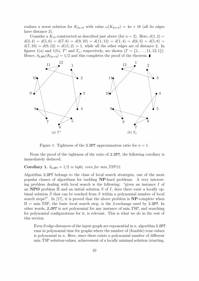
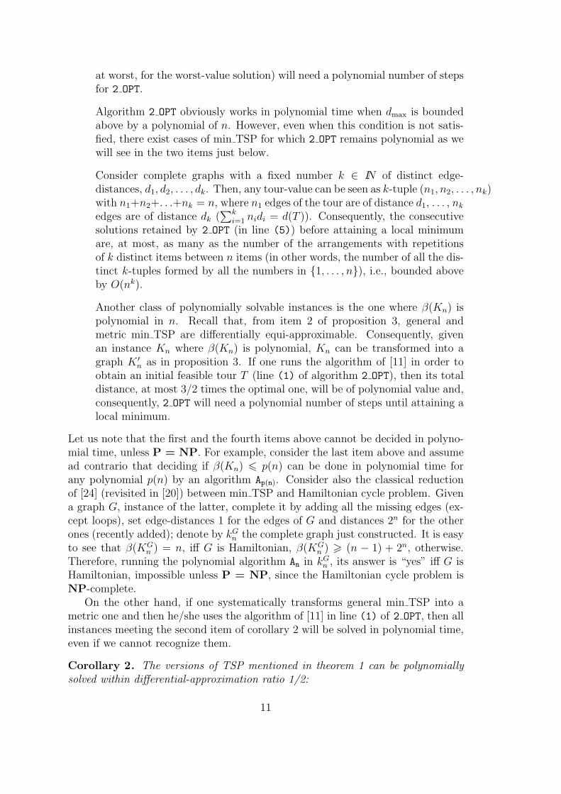
Consider a K12 constructed as described just above (for n = 2). Here, d(1, 2) =d(3, 4) = d(5, 6) = d(7, 8) = d(9, 10) = d(11, 12) = d(1, 4) = d(6, 3) = d(5, 8) =d(7, 10) = d(9, 12) = d(11, 2) = 1, while all the other edges are of distance 2. Infigures 1(a) and 1(b), T ∗ and Tω, respectively, are shown (T = {1, . . . , 11, 12, 1}).Hence, δ2 OPT(K2n+8) = 1/2 and this completes the proof of the theorem.

1

2

3

4

5

6

7

8

9

10

1112

(a) T ∗

12

3

4

5

6

7

8

9

10

11

12

(b) Tω

Figure 1: Tightness of the 2 OPT approximation ratio for n = 1.

From the proof of the tightness of the ratio of 2 OPT, the following corollary isimmediately deduced.

Corollary 1. δ2 OPT = 1/2 is tight, even for min TSP12.

Algorithm 2 OPT belongs to the class of local search strategies, one of the mostpopular classes of algorithms for tackling NP-hard problems. A very interest-ing problem dealing with local search is the following: “given an instance I ofan NPO problem Π and an initial solution S of I, does there exist a locally op-timal solution S that can be reached from S within a polynomial number of localsearch steps?”. In [17], it is proved that the above problem is NP-complete whenΠ = min TSP, the basic local search step, is the 2-exchange used by 2 OPT. Inother words, 2 OPT is not polynomial for any instance of min TSP, and searchingfor polynomial configurations for it, is relevant. This is what we do in the rest ofthis section.

Even if edge-distances of the input-graph are exponential in n, algorithm 2 OPT

runs in polynomial time for graphs where the number of (feasible) tour-valuesis polynomial in n. Here, since there exists a polynomial number of differentmin TSP solution-values, achievement of a locally minimal solution (starting,

10

at worst, for the worst-value solution) will need a polynomial number of stepsfor 2 OPT.

Algorithm 2 OPT obviously works in polynomial time when dmax is boundedabove by a polynomial of n. However, even when this condition is not satis-fied, there exist cases of min TSP for which 2 OPT remains polynomial as wewill see in the two items just below.

Consider complete graphs with a fixed number k ∈ IN of distinct edge-distances, d1, d2, . . . , dk. Then, any tour-value can be seen as k-tuple (n1, n2, . . . , nk)with n1+n2+. . .+nk = n, where n1 edges of the tour are of distance d1, . . . , nk

edges are of distance dk (∑k

i=1 nidi = d(T )). Consequently, the consecutivesolutions retained by 2 OPT (in line (5)) before attaining a local minimumare, at most, as many as the number of the arrangements with repetitionsof k distinct items between n items (in other words, the number of all the dis-tinct k-tuples formed by all the numbers in {1, . . . , n}), i.e., bounded aboveby O(nk).

Another class of polynomially solvable instances is the one where β(Kn) ispolynomial in n. Recall that, from item 2 of proposition 3, general andmetric min TSP are differentially equi-approximable. Consequently, givenan instance Kn where β(Kn) is polynomial, Kn can be transformed into agraph K ′

n as in proposition 3. If one runs the algorithm of [11] in order toobtain an initial feasible tour T (line (1) of algorithm 2 OPT), then its totaldistance, at most 3/2 times the optimal one, will be of polynomial value and,consequently, 2 OPT will need a polynomial number of steps until attaining alocal minimum.

Let us note that the first and the fourth items above cannot be decided in polyno-mial time, unless P = NP. For example, consider the last item above and assumead contrario that deciding if β(Kn) 6 p(n) can be done in polynomial time forany polynomial p(n) by an algorithm Ap(n). Consider also the classical reductionof [24] (revisited in [20]) between min TSP and Hamiltonian cycle problem. Givena graph G, instance of the latter, complete it by adding all the missing edges (ex-cept loops), set edge-distances 1 for the edges of G and distances 2n for the otherones (recently added); denote by kG

n the complete graph just constructed. It is easyto see that β(KG

n ) = n, iff G is Hamiltonian, β(KGn ) > (n − 1) + 2n, otherwise.

Therefore, running the polynomial algorithm An in kGn , its answer is “yes” iff G is

Hamiltonian, impossible unless P = NP, since the Hamiltonian cycle problem isNP-complete.

On the other hand, if one systematically transforms general min TSP into ametric one and then he/she uses the algorithm of [11] in line (1) of 2 OPT, then allinstances meeting the second item of corollary 2 will be solved in polynomial time,even if we cannot recognize them.

Corollary 2. The versions of TSP mentioned in theorem 1 can be polynomiallysolved within differential-approximation ratio 1/2:

11

on graphs where the optimal tour-value is polynomial in n;

on graphs where the number of feasible tour-values is polynomial in n (ex-amples of these graphs are the ones where edge-distances are polynomiallybounded, or even the ones where there exists a fixed number of distinct edge-distances).

4 An upper bound for the differential ratio of traveling

salesman

Remark first that for min TSP{ab} we have

ω (Kn) 6 bnβ (Kn) > an

}

=⇒ω (Kn)

β (Kn)6

b

a(8)

Suppose now that min TSP{ab} is approximable within differential ratio δ by apolynomial time approximation algorithm A. Then,

ω (Kn) − λA (Kn)

ω (Kn) − β (Kn)> δ =⇒ λA (Kn) 6 δβ (Kn) + (1 − δ)ω (Kn)

=⇒λA (Kn)

β (Kn)6 δ + (1 − δ)

ω (Kn)

β (Kn)

(8)

6b − (b − a)δ

a(9)

A corollary of the result of [16] is that min TSP cannot be approximated withinstandard-ratio 131/130− ε, ∀ε > 0. In the proof of this result, the authors considerinstances of min ∆TSP{ab} with a = 1 and b = 6 (in other words, the edge-distances considered are in {1, . . . , 6}). Revisit expression (9) and set a = 1, b = 6.Then solving inequality 6 − 5δ > 131/130 − ε with respect to δ, and taking intoaccount theorem 1, we get the following theorem.

Theorem 3. Neither the problems mentioned in theorem 1, nor min and max TSP{a, a+5}, min and max ∆αSTSP, min and max ∆αRTSP can be approximated withindifferential-ratio greater than, or equal to, 649/650 + ε, for every positive ε, unlessP=NP.

Recall now the result of [16], that min TSP12 cannot be approximated withinstandard-ratio smaller than 743/742−ε, ∀ε > 0. Using this bound in expression (9)(setting a = 1 and b = 2) and taking into account item 9 of proposition 3, thefollowing theorem holds.

Theorem 4. min and max TSPab, and min and max TSP12 are inapproximablewithin differential-ratio greater than, or equal to, 741/742 + ε, ∀ε > 0, unlessP=NP.

12

5 Standard-approximation results for relaxed and sharp-

ened maximum traveling salesman

5.1 Sharpened maximum traveling salesman

Consider an instance of ∆αSTSP and apply proposition 2 with γ = 1 and η =−2(1 − α)dmin. Then the instance obtained is also an instance of ∆TSP and,moreover, the two instances have the same set of feasible solutions.

Theorem 5. If max ∆TSP is approximable within standard-approximation ratio ρ,then max ∆αSTSP is approximable within standard-approximation ratio ρ + (1 −ρ)((1 − α)/α)2, ∀α, 1/2 < α 6 1.

Proof. Given an instance I = (Kn, ~d) of ∆αSTSP, we transform it into a ∆TSP-

instance I ′ = (Kn, ~d′) as described just above. As it has been already mentioned, Iand I ′ have the same set of feasible tours. Denote by T (I) and by T ∗(I) a feasibletour and an optimal tour of I, respectively, and by d(T (I)) and d(T ∗(I)) thecorresponding total lengths. Then, the total length of T in I ′ is d(T (I)) − 2n(1 −α)dmin.

Consider a PTAA for max ∆TSP achieving standard-approximation ratio ρ.Then, the following holds in I ′:

d(T (I)) − 2n(1 − α)dmin > ρ (d (T ∗(I)) − 2n(1 − α)dmin) (10)

In [8] it is proved that, for an instance of ∆αSTSP:

dmin >1 − α

2α2dmax (11)

and combining expressions (10) and (11), one easily gets

d(T (I)) > ρβ (I)+(1−ρ)

(

1 − α

α

)2

ndmaxndmax>β(I)

=⇒d(T (I))

β (I)> ρ+(1−ρ)

(

1 − α

α

)2

(12)completing so the proof of the theorem.

To our knowledge, no specific algorithm up to now is devised to solve max ∆TSPin standard approximation. On the other hand, being a special case of max TSP, max ∆TSPcan be solved by any algorithm solving the former within the same ratio. The bestknown such algorithm is the one of ([25]) achieving standard-ratio 3/4. Usingρ = 3/4 in expression (12), the following theorem holds and concludes the section.

Theorem 6. For every α ∈ (1/2, 1], max ∆αSTSP is approximable within standard-approximation ratio 3/4 + (1 − α)2/4α2.

5.2 Relaxed maximum traveling salesman

By theorems 1 and 2, max ∆αRTSP being equi-approximable to min TSP, it isapproximable within differential-approximation ratio 1/2. This fact, together withproposition 1, lead to the following theorem.

Theorem 7. max ∆αRTSP is approximable within standard-ratio 1/2, ∀α > 1.

13

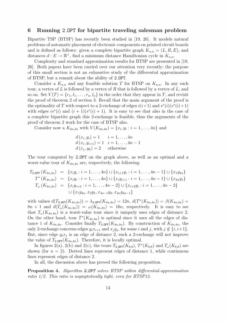
6 Running 2 OPT for bipartite traveling salesman problem

Bipartite TSP (BTSP) has recently been studied in [19, 26]. It models naturalproblems of automatic placement of electronic components on printed circuit boardsand is defined as follows: given a complete bipartite graph Kn,n = (L,R,E), anddistances d : E → R+, find a minimum distance Hamiltonian cycle in Kn,n.

Complexity and standard approximation results for BTSP are presented in [19,26]. Both papers have been carried over our attention very recently; the purposeof this small section is not an exhaustive study of the differential approximationof BTSP, but a remark about the ability of 2 OPT.

Consider a Kn,n and any feasible solution T for BTSP on Kn,n. In any suchtour, a vertex of L is followed by a vertex of R that is followed by a vertex of L, andso on. Set V (T ) = {r1, l1, . . . , rn, ln} in the order that they appear in T , and revisitthe proof of theorem 2 of section 3. Recall that the main argument of the proof isthe optimality of T with respect to a 2-exchange of edges i(i+1) and s∗(i)(s∗(i)+1)with edges is∗(i) and (i + 1)(s∗(i) + 1). It is easy to see that also in the case ofa complete bipartite graph this 2-exchange is feasible, thus the arguments of theproof of theorem 2 work for the case of BTSP also.

Consider now a K4n,4n with V (K4n,4n) = {xi, yi : i = 1, . . . , 4n} and

d (xi, yi) = 1 i = 1, . . . , 4nd (xi, yi+1) = 1 i = 1, . . . , 4n − 1d (xj, yk) = 2 otherwise

The tour computed by 2 OPT on the graph above, as well as an optimal and aworst-value tour of K4n,4n are, respectively, the following:

T2 OPT (K4n,4n) = {xiyi : i = 1, . . . , 4n} ∪ {xi+1yi : i = 1, . . . , 4n − 1} ∪ {x1y4n}

T ∗ (K4n,4n) = {xiyi : i = 1, . . . , 4n} ∪ {xiyi+1 : i = 1, . . . , 4n − 1} ∪ {x4ny1}

Tω (K4n,4n) = {xiyi+2 : i = 1, . . . , 4n − 2} ∪ {xi+2yi : i = 1, . . . , 4n − 2}

∪ {x1y4n, x2y1, x4n−1y2, x4ny4n−1}

with values d(T2 OPT(K4n,4n)) = λ2 OPT(K4n,4n) = 12n, d(T ∗(K4n,4n)) = β(K4n,4n) =8n + 1 and d(Tω(K4n,4n)) = ω(K4n,4n) = 16n, respectively. It is easy to seethat Tω(K4n,4n) is a worst-value tour since it uniquely uses edges of distance 2.On the other hand, tour T ∗(K4n,4n) is optimal since it uses all the edges of dis-tance 1 of K4n,4n. Consider finally T2 OPT(K4n,4n). By construction of K4n,4n, theonly 2-exchange concerns edges yixi+1 and xjyj, for some i and j, with j /∈ {i, i+1}.But, since edge yixj is an edge of distance 2, such a 2-exchange will not improvethe value of T2 OPT(K4n,4n). Therefore, it is locally optimal.

In figures 2(a), 2(b) and 2(c), the tours T2 OPT(K8,8), T ∗(K8,8) and Tω(K8,8) areshown (for n = 2). Dotted lines represent edges of distance 1, while continuouslines represent edges of distance 2.

In all, the discussion above has proved the following proposition.

Proposition 4. Algorithm 2 OPT solves BTSP within differential-approximationratio 1/2. This ratio is asymptotically tight, even for BTSP12.

14

x1

x2

x3

x4

x5

x6

x7

x8

y1

y2

y3

y4

y5

y6

y7

y8

(a) T2 OPT(K8,8)

x1

x2

x3

x4

x5

x6

x7

x8

y1

y2

y3

y4

y5

y6

y7

y8

(b) T ∗(K8,8)

x1

x2

x3

x4

x5

x6

x7

x8

y1

y2

y3

y4

y5

y6

y7

y8

(c) Tω(K8,8)

Figure 2: The tours T2 OPT(K8,8), T ∗(K8,8) and Tω(K8,8).

15

Finally note that the complexity of 2 OPT for BTSP is identical to the one forgeneral min or max TSP. Therefore the discussion of section 3 remains valid forthe bipartite case also.

7 Discussion: differential and deviation ratio

Revisit the deviation ratio as it has been defined and used in [18] for max TSP.There, the authors define a set Y of vertex-weight vectors ~y, the coordinates ofwhich are such that yi + yj 6 d(i, j), for ij ∈ E(Kn). Then,

zR = z∗ = max

{

2n

∑

i=1

yi : ~y = (yi) ∈ Y

}

(13)

Denote by ~y∗ the vector associated with z∗.In the same spirit, dealing with min TSP, the authors of [18] define a set W of

vertex-weight vectors ~w, the coordinates of which are such that wi + wj > d(i, j),for ij ∈ E(Kn). Then, zR = z∗ = min{2

∑n

i=1 wi : ~w = (wi) ∈ W}. Denote by ~w∗

the vector associated with z∗.Let us denote by Hmax (resp., Hmin) a heuristic for max TSP (resp., min TSP)

for which ρHmax= λHmax/β > ρ (resp., ρHmin = λHmin/β 6 ρ); H can stand for 2 OPT,

nearest neighbor (NN) (both 2 OPT and NN guarantee standard-approximation ra-tio 1/2 for max TSP), etc. Denote by MHmax the following algorithm running on agraph (Kn, ~d).

BEGIN /MHmax/

(1) FOR any distance d(i,j) DO d′(i, j) ← d(i, j) − yi − yj OD

(2) OUTPUT T ← Hmax(Kn, ~d′);

END. /MHmax/

Note that an analogous algorithm, denoted by MHmin, can be devised for min TSP ifone replaces the assignment in line (1) of algorithm MHmax by d′(i, j) ← wi + wj − d(i, j),and the algorithm Hmax called in line (2) by Hmin.

Fact 1. The tours computed by Hmax and Hmin are feasible. Moreover, given asolution T ′ computed by Hmax (resp., Hmin) in (Kn, ~d′), one recovers the cost ofa solution of the initial instance by adding quantity yi + yj to d′(i, j) (resp., byremoving d′(i, j) from wi + wj), ∀ij ∈ T ′.

Then, using fact 1, the following results are proved in [18].

Proposition 5. ([18]) Consider an instance (Kn, ~d) of max TSP (resp., min TSP)and an approximation algorithm Hmax (resp., Hmin) solving it within standard-approximationratio ρ. Then,

1. MHmax(Kn, ~d) produces a Hamiltonian tour satisfying λMHmax(Kn, ~d) > ρβ(Kn, ~d)+

(1 − ρ)2∑n

i=1 y∗

i = ρβ(Kn, ~d) + (1 − ρ)z∗;

16

2. MHmin(Kn, ~d) produces a Hamiltonian tour satisfying λMHmin(Kn, ~d) 6 ρβ(Kn, ~d)+

(1 − ρ)2∑n

i=1 w∗

i = ρβ(Kn, ~d) + (1 − ρ)z∗.

Obviously, algorithms MHmax, or MHmax, are not identical to Hmax, or Hmin, respec-tively; they simply use them as procedures. Hence, the nice results of [18] are not,roughly speaking, deviation-approximation results for say 2 OPT, or NN, when usedas subroutines in MHmax, or MHmin.

For max TSP, for example, it is easy to see that, instantiating H by 2 OPT, or NNand since the standard-approximation ratio of them is 1/2, application of item 1of proposition 5 leads to deviation ratios 1/2 for both of them. On the other hand,since these algorithms cannot guarantee constant standard-approximation ratiosfor min TSP ([24]), unless P=NP, max TSP and min TSP are not approximate-equivalent for the deviation ratio when z∗ and z∗ are used as reference values for theformer and the latter, respectively. Let us now focus ourselves on the max TSP andconsider algorithm MNNmax running on the following graph (K4n, ~d). Set V (K4n) ={x1, . . . , x2n, y1, . . . , y2n}. Set

d (yi, yj) = 1 i, j = 1, . . . , 2nd (xi, yi) = 1 i = 1, . . . , 2nd (xi, yj) = n otherwise

For this graph, we produce in what follows the tour TMNNmax(K4n) computed byalgorithm MNNmax, an optimal tour T ∗(K4n) and a worst-value tour Tω(K4n):

TMNNmax (K4n) = {xixi+1, yiyi+1 : 1 6 i 6 2n − 1} ∪ {x2ny1, y2nx1}

T ∗ (K4n) = {xiyi+1 : i = 1, . . . 2n − 1} ∪ {xiyi+2 : i = 1, . . . 2n − 2}

∪ {x2n−1y1, x2ny1, x2ny2} (14)

Tω (K4n) = {x2i−1y2i−1, y2i−1y2i, y2ix2i : i = 1, . . . , n} ∪ {x2ix2i+1 : i = 1, . . . , n − 1}

∪ {x2nx1} (15)

In other words, the following expressions hold for λMNNmax(K4n, ~d), ω(K4n, ~d) and β(K4n, ~d):

λMNNmax

(

K4n, ~d)

= λNNmax

(

K4n, ~d)

= (2n + 1)n + (2n − 1) = 2n2 + 3n − 1(16)

β(

K4n, ~d)

= 4n2 (17)

ω(

K4n, ~d)

= n2 + 3n (18)

From expression (16), one can see that running MNNmax on (K4n, ~d), or NNmax on (K4n, ~d)gives identical solution-values. In fact, by expression (13) (setting zi instead of yi),zR = z∗ = max{2

∑4n

i=1 zi : zi + zj 6 d(i, j)}. Moreover, in K4n,∑4n

i=1 zi =∑2n

i=1(zi + z2n+i) 6∑2n

i=1 d(xi, yi) = 2n. On the other hand, if we set zi = 1/2, weobtain z = 2

∑4n

i=1 zi = 4n. Consequently,

z = zR = 4n (19)

17

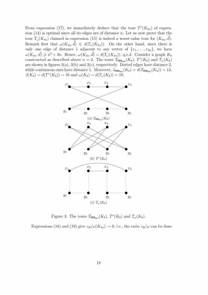
From expression (17), we immediately deduce that the tour T ∗(K4n) of expres-sion (14) is optimal since all its edges are of distance n. Let us now prove that the

tour Tω(K4n) claimed in expression (15) is indeed a worst-value tour for (K4n, ~d).

Remark first that ω(K4n, ~d) 6 d(Tω(K4n)). On the other hand, since there isonly one edge of distance 1 adjacent to any vertex of {x1, . . . , x2n}, we have

ω(K4n, ~d) > n2 + 3n. Hence, ω(K4n, ~d) = d(Tω(K4n)), q.e.d. Consider a graph K8

constructed as described above n = 2. The tours TMNNmax(K8), T ∗(K8) and Tω(K8)are shown in figures 3(a), 3(b) and 3(c), respectively. Dotted edges have distance 2,while continuous ones have distance 1. Moreover, λMNNmax(K8) = d(TMNNmax(K8)) = 13,β(K8) = d(T ∗(K8)) = 16 and ω(K8) = d(Tω(K8)) = 10.

x1x2 x3 x4

y1 y2 y3 y4

(a) TMNNmax(K8)

x1x2 x3 x4

y1 y2 y3 y4

(b) T ∗(K8)

x1x2 x3 x4

y1 y2 y3 y4

(c) Tω(K8)

Figure 3: The tours TMNNmax(K8), T ∗(K8) and Tω(K8).

Expressions (18) and (19) give zR/ω(K4n) → 0, i.e., the ratio zR/ω can be done

18

arbitrarily small. Combining expressions (16), (17), (18) and (19), one gets:

ρMNNmax

(

K4n, ~d)

=λMNNmax

(

K4n, ~d)

β(

K4n, ~d) →

1

2

δMNNmax

(

K4n, ~d)

=λMNNmax

(

K4n, ~d)

− ω(

K4n, ~d)

β(

K4n, ~d)

− ω(

K4n, ~d) →

1

3

dMNNmax

(

K4n, ~d, zR

)

=β

(

K4n, ~d)

− λMNNmax

(

K4n, ~d)

β(

K4n, ~d)

− zR

→1

2.

Moreover, algorithm NN could output the worst-value solution for some instances.From all the above, one can conclude that the fact that an algorithm achievesconstant deviation ratio does absolutely not imply that it simultaneously achievesthe same, or another constant, differential ratio.

Acknowledgment. The rigorous reading of the paper by two anonymous refereesand their very useful comments and suggestions are gratefully acknowledged. Manythanks to Anand Srivastav fore helpful discussions on bipartite TSP.

References

[1] A. Aiello, E. Burattini, M. Furnari, A. Massarotti, and F. Ventriglia. Com-putational complexity: the problem of approximation. In C. M. S. J. Bolyai,editor, Algebra, combinatorics, and logic in computer science, volume I, pages51–62, New York, 1986. North-Holland.

[2] T. Andreae and H.-J. Bandelt. Performance guarantees for approximationalgorithms depending on parametrized triangle inequalities. SIAM J. Disc.Math., 8:1–16, 1995.

[3] G. Ausiello, A. D’Atri, and M. Protasi. Structure preserving reductions amongconvex optimization problems. J. Comput. System Sci., 21:136–153, 1980.

[4] G. Ausiello, A. Marchetti-Spaccamela, and M. Protasi. Towards a unifiedapproach for the classification of NP-complete optimization problems. Theoret.Comput. Sci., 12:83–96, 1980.

[5] M. Bellare and P. Rogaway. The complexity of approximating a nonlinearprogram. Math. Programming, 69:429–441, 1995.

[6] M. A. Bender and C. Chekuri. Performance guarantees for the TSP with aparametrized triangle inequality. In Proc. WADS’99, volume 1663 of LectureNotes in Computer Science, pages 80–85. Springer, 1999.

19

[7] H.-J. Bockenhauer, J. Hromkovic, R. Klasing, S. Seibert, and W. Unger. To-wards the notion of stability of approximation algorithms and the travelingsalesman problem. Report 31, Electr. Colloq. Computational Comp., 1999.

[8] H.-J. Bockenhauer, J. Hromkovic, R. Klasing, S. Seibert, and W. Unger. Ap-proximation algorithms for the TSP with sharpened triangle inequality. In-form. Process. Lett., 75:133–138, 2000.

[9] H.-J. Bockenhauer, J. Hromkovic, R. Klasing, S. Seibert, and W. Unger. Animproved lower bound on the approximability of metric TSP and approxi-mation algorithms for the TSP with sharpened triangle inequality. In Proc.STACS’00, Lecture Notes in Computer Science, pages 382–394. Springer, 2000.

[10] H.-J. Bockenhauer and S. Seibert. Improved lower bounds on the approxima-bility of the traveling salesman problem. RAIRO Theoret. Informatics Appl.,34:213–255, 2000.

[11] N. Christofides. Worst-case analysis of a new heuristic for the traveling sales-man problem. Technical Report 388, Grad. School of Industrial Administra-tion, CMU, 1976.

[12] G. Cornuejols, M. L. Fisher, and G. L. Nemhauser. Location of bank accountsto optimize float: an analytic study of exact and approximate algorithms.Management Science, 23:789–810, 1977.

[13] A. Croes. A method for solving traveling-salesman problems. Oper. Res.,5:791–812, 1958.

[14] M. Demange, P. Grisoni, and V. T. Paschos. Differential approximation algo-rithms for some combinatorial optimization problems. Theoret. Comput. Sci.,209:107–122, 1998.

[15] M. Demange and V. T. Paschos. On an approximation measure founded onthe links between optimization and polynomial approximation theory. Theoret.Comput. Sci., 158:117–141, 1996.

[16] L. Engebretsen and M. Karpinski. Approximation hardness of TSP withbounded metrics. In Proc. ICALP’01, volume 2076 of Lecture Notes in Com-puter Science, pages 201–212. Springer, 2001.

[17] S. T. Fischer. A note on the complexity of local search problems. Inform.Process. Lett., 53:69–75, 1995.

[18] M. L. Fisher, G. L. Nemhauser, and L. A. Wolsey. An analysis of approxima-tions for finding a maximum weight Hamiltonian circuit. Oper. Res., 27:799–809, 1979.

[19] A. Frank, B. Korte, E. Triesch, and J. Vygen. On the bipartite travelingsalesman problem. Technical Report 98866-OR, University of Bonn, 1998.

20

[20] M. R. Garey and D. S. Johnson. Computers and intractability. A guide to thetheory of NP-completeness. W. H. Freeman, San Francisco, 1979.

[21] S. Lin and B. W. Kernighan. An effective heuristic algorithm for the travelingsalesman problem. Oper. Res., 21:498–516, 1973.

[22] C. H. Papadimitriou and S. Vempala. On the approximability of the travelingsalesman problem. In Proc. STOC’00, pages 126–133, 2000.

[23] C. H. Papadimitriou and M. Yannakakis. The traveling salesman problemwith distances one and two. Math. Oper. Res., 18:1–11, 1993.

[24] S. Sahni and T. Gonzalez. P-complete approximation problems. J. Assoc.Comput. Mach., 23:555–565, 1976.

[25] A. I. Serdyukov. An algorithm with an estimate for the traveling salesmanproblem of the maximum. Upravlyaemye Sistemy, 25:80–86, 1984.

[26] A. Srivastav, H. Schroeter, and C. Michel. Approximation algorithms for pick-and-place robots. Revised version communicated to us by A. Srivastav, April2001.

[27] S. A. Vavasis. Approximation algorithms for indefinite quadratic program-ming. Math. Programming, 57:279–311, 1992.

[28] E. Zemel. Measuring the quality of approximate solutions to zero-one pro-gramming problems. Math. Oper. Res., 6:319–332, 1981.

21