Approximation Algorithms for Two-State Anti-Ferromagnetic Spin Systems on Bounded Degree Graphs

J Stat Phys (2014) 155:666–686DOI 10.1007/s10955-014-0947-5

Approximation Algorithms for Two-StateAnti-Ferromagnetic Spin Systems on Bounded DegreeGraphs

Alistair Sinclair · Piyush Srivastava · Marc Thurley

Received: 19 December 2012 / Accepted: 4 February 2014 / Published online: 25 March 2014© Springer Science+Business Media New York 2014

Abstract We show that for the anti-ferromagnetic Ising model on the Bethe lattice, weakspatial mixing implies strong spatial mixing. As a by-product of our analysis, we obtain whatis to the best of our knowledge the first rigorous proof of the uniqueness threshold for theanti-ferromagnetic Ising model (with non-zero external field) on the Bethe lattice. Followinga method due to Weitz [15], we then use the equivalence between weak and strong spatialmixing to give a deterministic fully polynomial time approximation scheme for the partitionfunction of the anti-ferromagnetic Ising model with arbitrary field on graphs of degree atmost d , throughout the uniqueness region of the Gibbs measure on the infinite d-regular tree.By a standard correspondence, our results translate to arbitrary two-state anti-ferromagneticspin systems with soft constraints. Subsequent to a preliminary version of this paper, Sly andSun [13] have shown that our results are optimal in the sense that, under standard complexitytheoretic assumptions, there does not exist a fully polynomial time approximation scheme forthe partition function of such spin systems on graphs of maximum degree d for parametersoutside the uniqueness region. Taken together, the results of [13] and of this paper thereforeindicate a tight relationship between complexity theory and phase transition phenomena intwo-state anti-ferromagnetic spin systems.

Keywords Phase transitions · Complexity theory · Approximation algorithms ·Decay of correlations · Two-spin systems on trees

A preliminary version of this paper appeared in the proceedings of the 23rd Annual ACM-SIAM Symposiumon Discrete algorithms (SODA), pp. 941–953, 2012.

A. Sinclair · P. Srivastava (B)Soda Hall, University of California Berkeley, Berkeley, CA 94720, USAe-mail: [email protected]

A. Sinclaire-mail: [email protected]

M. ThurleyMedallia, Inc., Buenos Aires, Argentinae-mail: [email protected]

123

Approximation Algorithms for Two-State Spin Systems 667

1 Introduction

1.1 Background

Spin systems are a general framework for modeling nearest-neighbor interactions on graphs,and are widely studied in both statistical physics and applied probability. A spin systemconsists of a large collection of nodes, each of which may be in one of a fixed numberof states called spins. A neighborhood structure is specified by edges between the nodes.Interactions between neighboring nodes are determined by edge potentials, which assign anenergy value to each edge based on the spin values of its endpoints. In addition, there are vertexpotentials which assign an energy value to each node based on the value of its spin. For anyconfiguration σ of spins on the nodes, the energy H(σ ) is just the sum of its edge and vertexenergies. Based on the Gibbs formalism from statistical physics, the probability of findingthe system in configuration σ is then proportional to the weight w(σ) = exp(−H(σ )).

In this paper, we concentrate on two-state spin systems, where each vertex can be in oneof two states, referred to as “+” and “−”. Such a system can be defined by specifying a(+,+) edge activity β, a (−,−) edge activity γ , and a vertex activity λ, where β, γ and λare non-negative parameters. For a graph G = (V, E), a configuration σ : V → {+ ,− } isan assignment of + and − spins to the vertices of G. The weight w(σ) of the configurationσ is given by

w(σ) = λm(σ )βn+(σ )γ n−(σ ), (1)

where m(σ ) denotes the number of vertices assigned spin −, and n+(σ ) (respectively, n−(σ ))denotes the number of edges for which both endpoints are assigned spin + (respectively, −).The partition function of the model is defined as

Z =∑

σ∈{+,−}V

w(σ). (2)

The partition function, in addition to being a natural weighted generalization of the notion ofcounting, is a fundamental quantity in statistical physics. For example, it is the normalizingfactor in the Gibbs distribution: the probability of occurrence of configuration σ is givenby μ(σ) = w(σ)/Z . In addition, many other properties of the model can be deduced bystudying the partition function [4].

As a simple concrete example of a two-state spin system, consider the setting β = 1 andγ = 0 (so that configurations with adjacent “−” spins are assigned weight zero, and thusprohibited), known as the hard-core model. The associated Gibbs distribution is a weightedmeasure on independent sets in the graph G, in which any independent set U has weight λ|U |.Another important class of examples, known as the Ising model1, is obtained by settingβ = γ > 0. There is a significant qualitative difference between the Ising model withβ = γ > 1 (the ferromagnetic case) and with β = γ < 1 (the anti-ferromagnetic case).The latter is an example of a “repulsive” model, which means that the edge potentials assignhigher weights to edges with different spins at their endpoints, while the ferromagnetic case is“attractive” (higher weights are assigned to edges with the same spin at their endpoints). Theparameter λ can be identified with an “external field”, i.e., a bias associated with each spin.The case λ = 1 corresponds to zero field, while λ < 1 and λ > 1 correspond to positive andnegative fields respectively. More generally, we will refer to any two-state system satisfying

1 The description of the Ising model given here differs slightly from the more popular description in terms ofedge and vertex potentials outlined in the first paragraph. However, translating between the two descriptionsis easy; see Appendix 1.

123

668 A. Sinclair et al.

βγ > 1 as ferromagnetic, and any satisfying βγ < 1 as anti-ferromagnetic. Also, a modelsatisfying βγ > 0 is said to have soft constraints (in the sense that no combination of spinvalues at adjacent vertices is prohibited). In a sense to be made precise later (see Appendix 1),Ising models capture arbitrary two-state spin systems with soft constraints; in particular, thetwo descriptions are equivalent on regular graphs. For this reason we will henceforth focusmainly on Ising models.

The theory of spin systems derives in large part from considering the limiting behaviorof the Gibbs distribution as the size of the underlying graph goes to infinity. Based on theabove formalism for finite graphs, one may define a Gibbs measure μ on an infinite graphG by requiring that the marginal distribution on any finite subgraph H , conditional on theconfiguration on G \H , is given by Eq. (1). (Here the spins in G \H act as a fixed boundarycondition in (1).) It is a well known result in the statistical physics literature (see, for example,[4]) that at least one such measure μ can always be defined. However, for certain values ofthe parameters of the spin system there may be multiple solutions for μ, in which case theGibbs measure is said to be non-unique.

We will now look at the phenomenon of non-uniqueness more closely in the specialcase when the infinite graph G is a d-ary tree.2 As noted above, the anti-ferromagnetic Isingmodel essentially captures all two-state anti-ferromagnetic spin systems with soft constraintson regular graphs, and hence it is sufficient to consider the Ising case. Consider an anti-ferromagnetic Ising model on the d-ary tree with edge activity β(= γ ) and vertex activity λ.It turns out that if β ≥ d−1

d+1 then the Gibbs measure is unique for all values of λ. In particular,

in the zero-field case λ = 1, the Gibbs measure is unique if and only if β ≥ d−1d+1 . However,

when β < d−1d+1 , the Gibbs measure is no longer unique for all values of the vertex activity

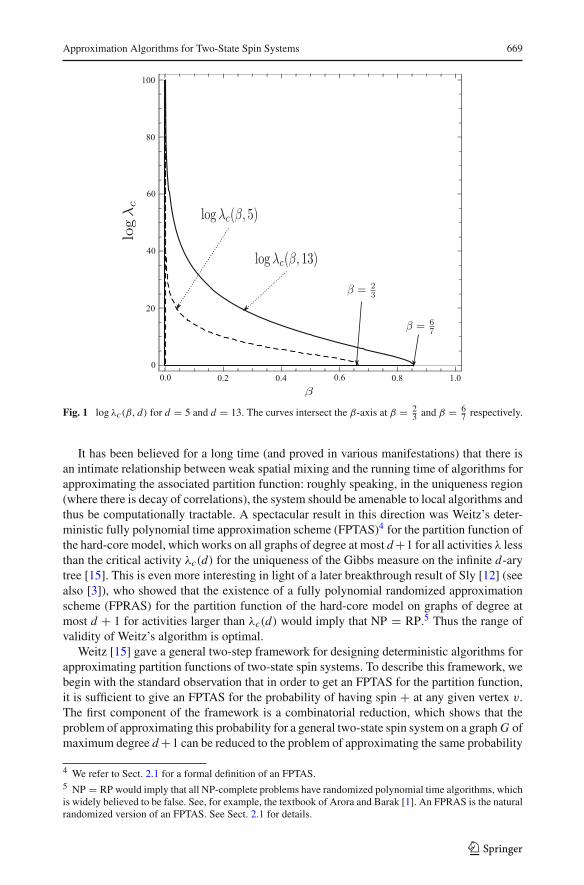
λ. In this case, there exists a critical activity λc (β, d) ≥ 1 such that the Gibbs measure isunique if and only if |log λ| ≥ log λc(β, d). We sketch the curves of log λc(β, d) in Fig. 1,for d = 5 and d = 13. The area below the curves is the non-uniqueness region. We notehere that the non-uniqueness region is monotonically increasing with degree, so the curvefor d = 5 lies strictly below that for d = 13. Also, note that the curves intersect the β-axisat β = d−1

d+1 .The phenomenon of non-uniqueness of the Gibbs measure can also be described in terms

of the more algorithmic notion of decay of correlations. We stick to our example of the infinited-ary tree. Fix a vertex v in the tree, and let Sl be the set of vertices in the tree at distanceat least l from v. Let qv(l, σ ) be the probability of having spin + at v conditional on theconfiguration on Sl being σ . It turns out that uniqueness of the Gibbs measure is equivalentto the condition that the inequality

|qv(l, σ )− qv(l, τ )| ≤ exp(−�(l)), (3)

holds for any two configurations σ and τ on Sl .3 The above condition is referred to in theliterature as weak spatial mixing.

2 We remark here that the infinite (d + 1)-regular tree (also known as the Bethe lattice) and the infinited-ary tree show exactly the same behavior with respect to the uniqueness of the Gibbs measure. This followsimmediately from the fact that the (d + 1)-regular tree can be viewed as a root attached to the roots of d + 1infinite d-ary trees. We shall thus move freely between these two objects for ease of exposition throughout thepaper.3 To be precise, this condition does not hold on the boundary of the uniqueness region, that is, for |log λ| =log λc(β, d); at this critical value, the l.h.s of Eq. (3) still decays to 0 with l, but not at an exponential rate.We will focus on the interior of this region, and by a slight abuse of terminology refer to it as the “uniquenessregion”.

123


Fig. 1 log λc(β, d) for d = 5 and d = 13. The curves intersect the β-axis at β = 23 and β = 6

7 respectively.

It has been believed for a long time (and proved in various manifestations) that there isan intimate relationship between weak spatial mixing and the running time of algorithms forapproximating the associated partition function: roughly speaking, in the uniqueness region(where there is decay of correlations), the system should be amenable to local algorithms andthus be computationally tractable. A spectacular result in this direction was Weitz’s deter-ministic fully polynomial time approximation scheme (FPTAS)4 for the partition function ofthe hard-core model, which works on all graphs of degree at most d +1 for all activities λ lessthan the critical activity λc(d) for the uniqueness of the Gibbs measure on the infinite d-arytree [15]. This is even more interesting in light of a later breakthrough result of Sly [12] (seealso [3]), who showed that the existence of a fully polynomial randomized approximationscheme (FPRAS) for the partition function of the hard-core model on graphs of degree atmost d + 1 for activities larger than λc(d) would imply that NP = RP.5 Thus the range ofvalidity of Weitz’s algorithm is optimal.

Weitz [15] gave a general two-step framework for designing deterministic algorithms forapproximating partition functions of two-state spin systems. To describe this framework, webegin with the standard observation that in order to get an FPTAS for the partition function,it is sufficient to give an FPTAS for the probability of having spin + at any given vertex v.The first component of the framework is a combinatorial reduction, which shows that theproblem of approximating this probability for a general two-state spin system on a graph G ofmaximum degree d +1 can be reduced to the problem of approximating the same probability

4 We refer to Sect. 2.1 for a formal definition of an FPTAS.5 NP = RP would imply that all NP-complete problems have randomized polynomial time algorithms, whichis widely believed to be false. See, for example, the textbook of Arora and Barak [1]. An FPRAS is the naturalrandomized version of an FPTAS. See Sect. 2.1 for details.

123


on a related finite subtree of the infinite (d + 1)-regular tree rooted at v, in which the spinsof some of the vertices are fixed to certain values (this is the so-called self-avoiding walktree of the graph G). We emphasize that this is a model-independent reduction, and dependsonly upon the fact that the number of spin values is two. The associated self-avoiding walktree, however, may be exponential in the size of the original graph G, and thus one needsto show that it is sufficient to truncate the tree at a depth logarithmic in the size of G inorder to obtain a good approximation. However, since some of the fixed vertices in the treemight be very close to the root v, it is not possible to argue using weak spatial mixing that alogarithmic depth of recursion suffices for approximating the partition function (because theparameter l in Eq. (3) must be taken to be the minimum distance of a fixed vertex from theroot).

Accordingly, the second component of Weitz’s framework is to establish that, for the spinsystem in question, weak spatial mixing on the infinite d-ary tree is in fact equivalent to strongspatial mixing, which roughly states that the exponential decay of point-to-set correlations (3)guaranteed by weak spatial mixing holds also when the spins at an arbitrary set of vertices arefixed to arbitrarily chosen values (see Sect. 2 for a precise definition). Weitz [15] establishedthis fact for the hard core model, using a step-by-step comparison of ratios of occupationprobabilities on the standard d-ary tree and on the modified tree with fixed vertices. It wasclaimed in [15] that such a result holds also for the anti-ferromagnetic Ising model, but tothe best of our knowledge no proof of this fact (except in the special zero-field case whereλ = 1; see [11,16]) has so far been published.

1.2 Contributions

In this paper, we give a proof of the fact that for the anti-ferromagnetic Ising model with anyfield, weak spatial mixing implies strong spatial mixing on the d-ary tree. Formally, we havethe following theorem.

Theorem 1 For the anti-ferromagnetic Ising model with arbitrary field on the d-ary treewith d ≥ 2, weak spatial mixing implies strong spatial mixing.

Remark We point out a byproduct of our approach that may be of independent interest. Theexact value of the critical field λc(β, d) as a function of (β, d) is apparently widely acceptedfolklore, but the only derivation we could find for it in the literature [4, p. 255] does notprovide a formal proof, appealing instead to numerical evidence. We emphasize that ourproof of strong spatial mixing does not assume knowledge of λc(β, d), and in fact derivesits value as a byproduct (see the Remark following Theorem 3 for more details). Thus ourapproach gives a proof of the location of the uniqueness threshold λc(β, d) of two-stateanti-ferromagnetic spin systems.

Notice that it is easy to see that in the statement of Theorem 1, “infinite d-ary tree” canbe replaced by “infinite (d + 1)-regular tree”, since the (d + 1)-regular tree and the d-arytree differ only in the degree of the root. Given Weitz’s general reduction described above,we obtain as an almost immediate consequence an FPTAS for the partition function of theanti-ferromagnetic Ising model on graphs of maximum degree at most d + 1 throughout theuniqueness region of the Gibbs measure on the d-ary tree.

Corollary 1 Let d ≥ 2. Consider an anti-ferromagnetic Ising model with parameters β andλ. For β and λ in the interior of the uniqueness region of the d-ary tree, every graph ofdegree at most d + 1 exhibits strong spatial mixing. Moreover, for such β and λ, there is a

123


deterministic fully polynomial time approximation scheme for the partition function of theassociated spin system on graphs of degree at most d + 1.

By the translation described in Appendix 1, we can extend this result to general two-stateanti-ferromagnetic spin systems. The difference is that the critical activity may now differ forvertices of different degrees. Let λc(β, d) be the critical activity for the anti-ferromagneticIsing model described above (and defined formally in Sect. 2.2.1). Then, we have the follow-ing corollary.

Corollary 2 Let d ≥ 2. Consider an anti-ferromagnetic two-state spin system with para-meters β, γ and λ. Let β ′ be the edge potential for the equivalent anti-ferromag-netic Isingmodel. Let G be the class of graphs with maximum degree d + 1 in which every vertex vsatisfies the condition

| log λv| �∣∣∣∣log λ+ deg(v)

2(log γ − logβ)

∣∣∣∣ > log λc(β′, d).

Then there is a deterministic fully polynomial time approximation scheme for the partitionfunction of the associated spin system on graphs in the class G . In particular, the class Gincludes all (d + 1)-regular graphs when β, γ and λ are in the interior of the uniquenessregion of the d-ary tree.

We briefly sketch the approach we use to prove our main technical result, namely thatweak spatial mixing implies strong spatial mixing (Theorem 1). Inspired by recent work ofRestrepo et al. [11], we design a “message” (i.e., an invertible function of the probability ofa vertex having spin + ) such that “disagreements” in the message decay by a constant factorat each vertex of the tree. The challenge is to ensure that such a message can be designedfor all points in the uniqueness region of the d-ary tree. For the special zero-field case of theanti-ferromagnetic Ising model (when λ = 1), such a message is well known [16]. However,this message does not work up to the threshold for general vertex potentials λ. Restrepo etal. [11] recently derived a message which works up to the tree uniqueness threshold for thehard-core model. For the general anti-ferromagnetic Ising model, such a message turns out tobe more complex than those known for the zero-field case and for the hard-core model. Ourmessage is defined at the beginning of Sect. 3, and the requisite decay property is establishedin Sect. 4.

We conjecture that our proof of strong spatial mixing based on stepwise decay of messagesmay lead to further consequences. For example, as shown by Restrepo et al. [11], the messagedecay property can be used to extend Weitz’s algorithm by exploiting the structure of specialclasses of graphs to obtain approximation algorithms beyond the tree threshold for thosegraphs. In addition, our proof demonstrates the versatility of the message approach introducedby Restrepo et al.

Remark After obtaining our message-decay proof, we received a sketch of Weitz’s orig-inal unpublished proof [14]. It is interesting to note that that proof is quite differentfrom ours, and employs a delicate two-step analysis of the tree recursion described inSect. 2. For reasons mentioned above, we believe that our message-decay proof, in addi-tion to being the first published version of this result, is potentially more robust andflexible than Weitz’s approach; for example, it is not clear how to adapt Weitz’s analy-sis to obtain stronger results for special classes of graphs such as lattices, as is done in[11].

123


1.3 Related Work

Our work is mainly motivated by the deterministic counting algorithm of Weitz [15], whichwas the first to show an interesting connection between the running time of an algorithmnot related to Markov chain Monte Carlo and the phase transition phenomenon for spinsystems. On the complexity side, using a randomized gadget first proposed by Dyer, Friezeand Jerrum [2] and analysed further by Mossel, Weitz and Wormald [10], Sly [12] provedthat if there is an FPRAS for the partition function of the hard-core model on graphs ofdegree at most d in the non-uniqueness region of the d-regular tree, then NP = RP, thusshowing that the range of validity of Weitz’s algorithm is optimal. Technically Sly’s resultholds only sufficiently close to the boundary of the uniqueness region; this restriction wasmostly removed in a later paper of Galanis et al. [3].

For two-state anti-ferromagnetic spin systems on unbounded degree graphs, Goldberg,Jerrum and Paterson [6] showed that approximating the partition function for the zero-fieldcase (λ = 1) is NP-hard in the interior of the square 0 ≤ β, γ ≤ 1. For bounded degreegraphs, subsequent to the results of this paper, Sly and Sun [13] have shown that there is noFPRAS for the partition function of the anti-ferromagnetic Ising model on d-regular graphsin the non-uniqueness regime of the d-regular tree, unless NP = RP. The results of [13]taken together with the results of this paper therefore strengthen the connections between thetheory of NP-hardness and the phase transition phenomenon first established by the resultsof Weitz [15] and Sly [12] cited above.

A related problem is to get exponential lower bounds on the mixing time of any localMarkov chain (Glauber dynamics) that samples from the hard-core and anti-ferromagneticIsing models. Mossel, Weitz and Wormald [10] and Gerschenfeld and Montanari [5] showedthat beyond the uniqueness threshold for d-regular trees, Glauber dynamics for these modelscan take exponential time to mix on d-regular graphs. Gerschenfeld and Montanari also showthat for these models on random regular graphs, this threshold for slow mixing is also thethreshold beyond which the reconstruction problem on the graph is solvable.

On the algorithmic side, an analysis of Weitz’s algorithm for the zero-field case of theanti-ferromagnetic Ising model appears in [16]. There has been some subsequent progresson the hard-core model on special classes of graphs too: recently, Restrepo et al. [11] used amessage-decay proof to get improved strong spatial mixing thresholds on the 2D integerlattice for the hard core model. They achieved this by exploiting the special structure of self-avoiding walk trees obtained when Weitz’s reduction is applied to the lattice. The message-decay proof turns out to be crucial in tightening the analysis to obtain strong spatial mixingover a wider range of parameters for these special trees. Much more is known about algorithmsfor the ferromagnetic case: Jerrum and Sinclair [7] gave an FPRAS for the Ising modelwith arbitrary field on graphs of arbitrary degree, while Goldberg, Jerrum and Paterson [6]showed how to extend this to the whole of the ferromagnetic region βγ > 1 with λ = 1.The latter paper [6] also gave an FPRAS for the partition function on graphs of arbitrarydegree for parts of the anti-ferromagnetic region βγ < 1. However, the results of [6] whenrestricted to bounded degree graphs do not hold throughout the uniqueness region and henceare incomparable to ours.

More recently, the work of [6] has been improved upon by Li, Lu and Yin [9]. Theyconsider two-state anti-ferromagnetic spin systems with zero field (λ = 1) on general graphs,and derive a condition under which an FPTAS exists for approximating the partition function.Their condition requires that (β, γ ) lies in the intersection of the uniqueness regions for allpossible degrees d . (Note that in the (β, γ ) parameterization, this is a non-trivial region ofthe βγ -plane.) However, for any fixed degree d , this region is smaller than the uniqueness

123


region for d , which is the range of validity obtained in our present paper. We also point outan important qualitative difference between the parameterization we use (edge potential βand vertex field λ) and the parameterization via two edge potentials (β and γ ) used by Li etal.: while the (β, γ ) parametrization is not monotonic, in the sense that uniqueness on a d-regular tree does not imply uniqueness on a (d −1)-regular tree, the (β, λ) parametrization ismonotonic. In fact, as our results show, uniqueness on the d-regular tree implies strong spatialmixing, and hence uniqueness, on all d ′-regular trees for d ′ ≤ d in the (β, λ) parametrization.Subsequent to the results of this paper, Li, Lu and Yin [8] have presented a unified frameworkfor establishing the results of this paper as well as their earlier paper [9]; their new approachalso improves upon our Corollary 2 in the case of non-regular graphs.

2 Preliminaries

2.1 Notation and Terminology

We will mostly follow the notational conventions of [6]. Given a graph G = (V, E), a two-state spin configuration is defined as an assignment σ : V → {+ ,− } of spins to the vertices.Weights for different configurations are computed in terms of the (+,+)-edge activity β, the(−,−) edge activity γ and a vertex activity λ, and are given by

w(σ) = λm(σ )βn+(σ )γ n−(σ ), (4)

where given the configuration σ , m(σ ) denotes the number of vertices assigned spin −,and n+(σ ) (respectively, n−(σ )) denotes the number of edges for which both endpoints areassigned spin + (respectively, −). The partition function is defined as

Z =∑

σ∈{−1,1}V

w(σ).

We remark that this representation can be easily translated to the usual description in termsof edge potentials and vertex field: for completeness we give the translation in Appendix 1.

Definition 1 (Occupation probability) Given a vertex v in the graph G, the occupationprobability pv is the probability that v is assigned spin + in a random configuration σsampled according to the weights defined in Eq. (4).

The standard notion of efficient approximation in complexity theory is that of a fullypolynomial time approximation scheme, which we define below in relation to the computationof the partition function.

Definition 2 (Fully polynomial time approximation scheme) Consider a two state spinsystem with parameters β, γ and λ. A deterministic algorithm A for approximating the par-tition function Z of the model is called a fully polynomial approximation scheme (FPTAS) if,given an input graph G and accuracy parameter ε > 0, the algorithm runs in time polynomialin 1/ε and the size of the graph G and outputs a quantity Z satisfying

(1 − ε)Z ≤ Z ≤ (1 + ε)Z . (5)

A closely related notion is that of a fully polynomial randomized approximation scheme(FPRAS). In this case, the algorithm A is a randomized algorithm, and takes as input a graphG, an accuracy parameter ε > 0 and a confidence parameter δ > 0, runs in time polynomialin 1/ε, log(1/δ) and the size of the graph G, and outputs a quantity Z which satisfies thecondition in Eq. (5) with probability at least 1 − δ.

123


2.2 The Ising Model

The Ising model corresponds to the case β = γ . The model is ferromagnetic when β > 1 andanti-ferromagnetic when β < 1 (the case β = 1 is trivial). The zero-field case correspondsto λ = 1, the positive field case to λ < 1 and the negative field case to λ > 1. As shownin Appendix 1, on d-regular graphs the Ising model is equivalent to general two-state spinsystems. Thus, in the rest of this paper, we will concentrate mostly on the Ising case. Onnon-regular graphs the equivalence still holds; however, the vertex activity λ in the Isingmodel may then be different on different vertices. The adaptation of our results to this settingis described in Corollary 2.

2.2.1 Phase Transition

The anti-ferromagnetic Ising model exhibits a uniqueness phase transition on the d-ary treefor d ≥ 2. In particular, one can show the existence of a critical activity λc(β, d) as expressedin the following classical result (see, e.g., Georgii [4, p. 254]).

Theorem 2 (Existence of a critical activity) Consider the anti-ferromagnetic Ising modelon an infinite d-ary tree with edge activity β and vertex activity λ. If β ≥ d−1

d+1 then the

Gibbs measure is unique for all values of λ. If β < d−1d+1 , then there exists a critical activity

λc(β, d) ≥ 1 such that the Gibbs measure is unique if and only if |log λ| ≥ log λc(β, d).

A consequence of uniqueness6 of the Gibbs measure is weak spatial mixing, which captures aweak notion of decay of point to set correlations. Let pρ(σ, S) be the probability of occupationof the root ρ of an infinite d-ary tree when the spins of a set S of nodes are fixed accordingto the configuration σ . Let δ(ρ, S) denote the distance of ρ from the set S.

Definition 3 (Weak spatial mixing) Given any two-state spin system, weak spatial mixingis said to hold if for any set S whose distance δ(ρ, S) from the root ρ of the tree is finite, andany two configurations σ1 and σ2, we have

|pρ(σ1, S)− pρ(σ2, S)| ≤ exp(−�(δ(ρ, S))).

Notice that weak spatial mixing does not guarantee exponential decay of correlations whenthe set S contains vertices which are very close to the root ρ, even when σ1 and σ2 differ onlyon vertices which are very far away from ρ. A related but, as the name suggests, strongernotion is that of strong spatial mixing, which captures the idea that fixing vertices near theroot to the same spin should not affect the exponential decay of point-to-set correlations. Wenote that strong spatial mixing is not in general implied by weak spatial mixing for arbitraryspin systems; see Appendix 2 for a counterexample involving the ferromagnetic Ising modelwith appropriate parameters.

Definition 4 (Strong spatial mixing) Given any two-state spin system, strong spatial mixingis said to hold if for any set S whose distance δ(ρ, S) from the root ρ of the tree is finite, andany two configurations σ1 and σ2 which differ only on a set T ⊆ S of vertices, we have

|pρ(σ1, S)− pρ(σ2, S)| ≤ exp(−�(δ(ρ, T ))).

6 As stated in the introduction, we exclude the boundary of the uniqueness region here.

123


2.2.2 Phase Transition and Tree Recursions

It is well known (see, for example, [4]) that the uniqueness condition for two-state spinsystems on d-ary trees can be written in terms of the number of fixed points of the recursionfor occupation probabilities. Consider a subtree rooted at a vertex v in the d-ary tree, and letvi , i = 1, 2, ...d be its children. Let pv be the occupation probability at vertex v and defineRv = 1−pv

pv. One can then write the following recurrence for Rv :

Rv = λ

d∏

i=1

(βRvi + 1

β + Rvi

).

This can easily be converted to a recurrence for occupation probabilities. Define

h(x) �β + (1 − β)x

1 − (1 − β)x.

We can then write the recurrence as

pv = F(pv1 , pv2 , . . . , pvd ) �1

1 + λ∏d

i=1 h(pvi ). (6)

We will find it useful in what follows to consider the tree recurrence with the special boundarycondition in which all vertices at some distance l from the root are fixed to the same spin.In this case, by symmetry, the tree recurrence outputs the same value pv at all vertices vwhich are at the same distance from the root. Thus, the recurrence can be simplified to aone-parameter recurrence as follows:

pv = f (pv1) �1

1 + λh(pv1)d.

Note that in the anti-ferromagnetic case, h is an increasing function, and hence F and fare decreasing in each of their arguments. We also note that since f is strictly decreasing in[0, 1], it has a unique fixed point.

In terms of the recurrence function f , the condition for uniqueness can be stated as follows.

Theorem 3 ([4]) For given values of β and λ, the infinite d-ary tree has a unique Gibbsmeasure if and only if the two-step recurrence function f ◦ f has a unique fixed point.In particular, if the Gibbs measure is unique, and (β, λ) are not on the boundary of theuniqueness region, then the unique fixed point x� of f satisfies

f ′(x�) > −1. (7)

Remark In [4], it is claimed (implicitly) on the basis of numerical simulations that thecondition (7) is also sufficient for uniqueness. To be precise, the expression for the criticalactivity λc(β, d) given in [4, p. 255] is exactly the same as that obtained by assuming that(7) is also a sufficient condition for uniqueness. While we believe this fact to be folklore,we have not been able to find a rigorous proof of it in the literature. With a slight abuseof terminology, we will henceforth refer to the set of (β, λ) for which the fixed point x�

satisfies f ′(x�) > −1 as the “uniqueness region”. We will justify this terminology later (seethe Remark following the proof of Theorem 1 in Sect. 4) by proving that condition (7) doesindeed imply uniqueness. Thus we will obtain a rigorous proof of the expression for thecritical activity appearing in [4].

123


2.3 Messages

Definition 5 (Message) A message is a continuously differentiable function φ : [0, 1] → R

with positive derivative.

Note that a message is strictly increasing and hence invertible on its range. Moreover, theinverse function φ−1 is also a continuously differentiable function with positive derivative.

Given a recurrence function f : [0, 1] → [0, 1], and a message φ, we denote by f φ thefunction φ ◦ f ◦φ−1. The function f φ , which will play a crucial role in this paper, describesthe evolution of the message φ under the recurrence, in the sense that f φ(φ(x)) = φ( f (x)).We will also need the following fact.Notation In the following, we will find it convenient to use the following shorthand notations:we will denote the function f φ as g, and the inverse φ−1 of φ as ψ .

Fact 4 For any message φ, the parameters (β, λ) are in the uniqueness region if and only ifg′(p�) > −1 at the unique fixed point p� of g = f φ .

Proof Notice that since φ is strictly increasing, and f has a unique fixed point x�, g = f φ

also has a unique fixed point p� = φ(x�). Now, we notice that g′(p�) = f ′(x�), because

g′(p�) = φ′( f (ψ(p�))) f ′(ψ(p�))ψ ′(p�)

= φ′( f (x�)) f ′(x�) 1

φ′(ψ(p�))

= φ′(x�)φ′(x�)

f ′(x�)

= f ′(x�),

where in the second line we used the facts that ψ(p�) = x� and ψ ′(y) = 1φ′(ψ(y)) , and in the

third line the fact that f (x�) = x�. Thus, (β, λ) are in the uniqueness region (as defined inthe Remark following Theorem 3) if and only if g′(p�) = f ′(x�) > −1.

2.4 Weitz’s Tree Reduction

As indicated in the introduction, Weitz [15] proved the following combinatorial reduction(see [15] for a formal definition of the self-avoiding walk tree used in this theorem).

Theorem 5 ([15]) Let G be a graph of degree at most d, and let v be a vertex in G. For anytwo-state spin system on G, the occupation probability pv in (G) is equal to the occupationprobability of v in the self-avoiding walk (SAW) tree (which is also of degree at most d) rootedat v. Further, if the SAW tree exhibits strong spatial mixing, then there is a deterministic fullypolynomial time approximation scheme for the partition function of the spin system on graphsof degree at most d.

3 Messages and Contraction on the d-ary Tree

In this section, we will prove the main technical ingredient of our result, which is expressedin the following theorem.

Theorem 6 Given d, β and λ, there exists a message φ and a constant c < 1, such that thetree recurrence g = f φ for the quantity φ(pv) satisfies ‖g′‖∞ ≤ c < 1, whenever (β, λ) isin the uniqueness region for the d-ary tree.

123


The above theorem says that in the uniqueness region, the single-parameter recurrence g =f φ for the message φ(pv) contracts at every step. (Without the message, the function f itselfis not contractive.) This stepwise contraction is easily seen by standard arguments to implyweak spatial mixing; for completeness, we give a proof in the Section titled “Contraction andWeak Spatial Mixing” in Appendix 3. To extend the argument to strong spatial mixing, asrequired for Theorem 1, we need to consider a multi-parameter (vectorized) version of themessage recurrence g, since under arbitrary boundary conditions the occupation probabilitiesneed not be uniform. We will show in Sect. 4 that for our messageφ in Theorem 6, the analysisof the vectorized version can in fact be reduced to an application of Theorem 6.

Remark For ease of notation, in the rest of the paper we will prove our results in terms of theuniqueness threshold of the d-ary tree, relating it to algorithms on graphs of degree at mostd + 1. As already noted, the uniqueness thresholds on the (d + 1)-regular tree and the d-arytree coincide, and hence our results apply equally to the infinite (d + 1)-regular tree.

We begin by setting up some notation for the proof of Theorem 6. In light of Fact 4,the main technical challenge is to come up with a message φ such that the quantity

∣∣g′∣∣ ismaximized at the unique fixed point of g = f φ . Let us fix constants

A = d(1 − β2)+ (1 − β)2 and D =√

A + 4β − √A

2√

A.

Define

φ(x) = log

(x + D

1 − x + D

).

Notice that D > 0, so φ is a continuously differentiable function with positive derivativeon the interval [0, 1]. Using this message we are able to prove the following (recall that ψdenotes φ−1).

Lemma 1 Consider the anti-ferromagnetic Ising model on a d-ary tree with edge activity βand vertex activity λ. Then, using the shorthand notations α and η for ψ(x) and f (ψ(x))respectively, we have

g′′(x) = (η − α)g′(x)ψ ′(x)

× dβ(1 − β2)(2β + Aαη + A(1 − α)(1 − η))

(β + α(1 − α)(1 − β)2)(β + Aη(1 − η))(β + Aα(1 − α)). (8)

The proof of Lemma 1 is somewhat technical and is deferred to Sect. 5.Before proceeding with the technical development, we pause to give some comments on the

design of our message. Notice that the requirement that the derivative of the function g = f φ

should have its maximum magnitude at the unique fixed point of g does not immediately leadto a solution for φ, and thus we must resort to some educated guesswork for the functionalform of φ. Our choice is guided by the intuition that, by analogy with the zero field case,

where it is well known that the simple message φ(x) = log(

x1−x

)is sufficient, a log ratio of

probabilities shifted by an additive constant D to account for the field should be appropriate.The choice of D is then determined by the above requirement. An important additionalproperty of our message is that, perhaps surprisingly, it does not depend upon the vertexpotential λ, but only upon the edge potential β and the degree d; this is reflected in the factthat the additive shift D is the same for both probabilities. This property will be important inextending our algorithm to the setting of general two-state anti-ferromagnetic spin systemsin Corollary 2.

123


Lemma 2 Let g = f φ , with the message φ defined above. Then |g′(x)| is maximized at theunique positive fixed point of g.

Proof We use the notation established in Lemma 1, where we derived an expression for g′′(x)in Eq. (8). It is easy to see that ignoring the factor (η − α), the rest of the right hand side ofEq. (8) is negative: this is because g is a decreasing function, while ψ , being the inverse ofthe increasing function φ, is increasing. Also, we have 0 < β < 1 (in the anti-ferromagneticcase) and 0 ≤ α, η ≤ 1 (since they are probabilities), so that the fractions appearing on theright hand side are positive.

Let x� be the unique fixed point of the strictly decreasing function g. From the abovediscussion, it follows that the sign of g′′(x) is the opposite of the sign of η−α = f (ψ(x))−ψ(x). Notice that η − α is strictly positive for x < x� and strictly negative for x > x�. Thisimplies that g′(x) is strictly decreasing for x < x� and strictly increasing for x > x�. Sinceg is strictly decreasing this shows that the magnitude of g′ is maximized at x�.

Combining Lemma 2 with Fact 4, we immediately get Theorem 6. Lemma 2 further impliesthat the constant c in the Theorem is |g′(x�)|, where x� is the unique fixed point of g.

4 Strong Spatial Mixing on the d-ary Tree

In this final section we use the message defined in the previous section to prove our mainresult, Theorem 1. Along with Weitz’s reduction stated in Theorem 5, this will immediatelyimply Corollary 1, the FPTAS for the anti-ferromagnetic Ising model with arbitrary fields. Toderive Corollary 2 for general two-state spin systems, we will need the translation describedin Appendix 1. Both these latter proofs appear at the end of this section.

Recall that Theorem 1 asserts that weak spatial mixing implies strong spatial mixing. Wealready showed in Theorem 6 that in the uniqueness region, there is uniform contraction inthe tree recurrence with uniform boundary conditions. However, in order to prove strongspatial mixing, we will need to handle non-uniform boundary conditions as well, in whichcase the one-parameter recurrence g = f φ is no longer sufficient. We therefore consider themulti-parameter vectorized version G of the function g. For x ∈ R

d , G(x) is defined as

G(x1, x2, . . . , xd) = φ

(1

1 + λ∏d

i=1 h (ψ(xi ))

), (9)

where, as before, ψ = φ−1. We claim that strong spatial mixing on the d-ary tree is impliedwhenever the function G satisfies the following condition; a proof of this implication can befound in the Section titled “Contraction and Strong Spatial Mixing” in Appendix 3.

Definition 6 (Contractive spatial mixing) Given the parameters β and λ for the anti-ferromagnetic Ising model on a d-regular tree, contractive spatial mixing holds if there existsa constant c < 1 such that

|G(x)− G( y)| ≤ c‖x − y‖∞,

for the vectorized version G of g defined as above with respect to the message φ.

To establish this condition, we will rely on the following lemma.

Lemma 3 Let η = ψ(G(x)). Let η be the unique solution of ψ(g(η)) = η. Then‖∇G(x)‖1 ≤ ‖∇G(η, η, . . . , η)‖1 = |g′(η)|.

123


Proof Set αi = ψ(xi ) for i = 1, 2, . . . d . We then have

η = 1

1 + λ∏d

i=1 h(αi )= 1

1 + λh(ψ(η))d. (10)

Recalling the definitions of the quantities A and D given just before Lemma 1, we can nowwrite ‖∇G(x)‖1 as

‖∇G(x)‖1 = dη(1 − η)(1 − β2)

β + Aη(1 − η)

(1 + (1 − β2)

d∑

i=1

αi (1 − αi )

β + (1 − β)2αi (1 − αi )

). (11)

For notational convenience, we define the function J (x) � x(1−x)β+(1−β)2x(1−x)

. Note that max-

imizing the sum in (11) under the constraint (10) is the same as maximizing∑d

i=1 J (αi )

under the constraint that∏d

i=1 h(αi ) = 1−ηλη

. Since h is positive and invertible, it is therefore

sufficient to show that the function K (x) � J (h−1(ex )) is concave in order to show that allαi ’s are equal at a maximum. We now show this by direct computation. After differentiatingtwice and simplifying, we have

K ′′(x) = −e−x (1 + e2x )β

(1 − β2)2< 0.

This shows that K is concave. By the discussion above, it follows that the sum in Eq. (11)is maximized when all αi ’s are equal. In conjunction with the condition that η = 1

1+∏di=1 h(αi )

,

this shows that

‖∇G(x)‖1 ≤ ‖∇G(η, η, . . . , η)‖1.

Note that for any x , G(x, x, ..., x)=g(x), and therefore ‖∇G(η, η, . . . , η)‖1 =|g′(η)|.Using Lemma 2 and the above lemma, we are now ready to prove our main technical

result, Theorem 1, which says that weak spatial mixing implies strong spatial mixing forgeneral anti-ferromagnetic Ising models.

Proof of Theorem 1 Consider a setting of parameters β and λ such that the d-ary tree hasweak spatial mixing. Let x� be the unique fixed point of the function g. We will use onlythe property that the fixed point satisfies the condition (7) of Theorem 3. By Theorem 6 wehave ‖g′‖∞ = c < 1. By Lemma 3, this implies that for all x in the domain of the functionG defined in Eq. (9), ‖∇G(x)‖1 ≤ c. Using the mean value theorem followed by Hölder’sinequality, we then have

|G(x)− G( y)| ≤ c‖x − y‖∞,

for all vectors x and y in the domain of G, and thus contractive spatial mixing holds. Asobserved above, this implies strong spatial mixing.

Remark We can now justify our use of the term “uniqueness region” as described in theRemark following Theorem 3. Notice that in the proof of Theorem 1 above, we used only thefact that weak spatial mixing implies that (β, λ) is in the “uniqueness region” as defined inthe aforementioned Remark. Thus, we see that whenever (β, λ) is in the uniqueness region,we have strong spatial mixing, and hence, in particular, uniqueness. As stated earlier, thisprovides a rigorous proof of the claim in [4] that the interior of the uniqueness region isequivalent to the condition (7).

123


Combining the above theorem with the general reduction of Weitz [15] stated in Theorem 5,we can now prove Corollary 1, which asserts the existence of an FPTAS for general anti-ferromagnetic Ising models on bounded-degree graphs up to the uniqueness threshold.

Proof of Corollary 1 As observed earlier, in order to obtain an FPTAS for the partition func-tion of the associated spin system, it is sufficient to give an FPTAS for approximating theoccupation probability pρ of a vertex ρ, under an arbitrary fixing of spin values for an arbi-trary subset of vertices. Given a vertex ρ in a graph G of maximum degree (d +1), we start byconstructing Weitz’s self-avoiding walk (SAW) tree rooted at ρ. For non-leaf vertices (apartfrom ρ) in this tree which do not have d children, we can create dummy children (so as tomake the arity of the vertex d) all of which independently have occupation probabilities of1/2. It is easy to see that this does not change the output of the tree recurrence (Eq. (6)) at anyvertex of the tree. As we saw in the proof of Theorem 1, we have strong spatial mixing onthis SAW tree whenever (β, λ) are in the uniqueness region of the d-ary tree. The corollarynow follows using Weitz’s reduction (Theorem 5).

Finally, we will see how to use Lemmas 1 and 3 to prove Corollary 2, which extends theFPTAS to general two-state anti-ferromagnetic spin systems.

Proof of Corollary 2 Given a two-state spin system with parameters β, γ and λ on a graphG of degree at most d + 1, we can use the translation given in Appendix 1 to come up withan equivalent Ising model with edge potential β ′ = √

βγ and vertex-dependent potentialsλv = λ(

√γ /β)dv . Now, as before, in order to estimate the occupation probability pρ for a

given vertex ρ, we construct Weitz’s self-avoiding walk (SAW) tree rooted at ρ, and completethe degree of any non-leaf vertex (apart from ρ) in the tree which does not have d childrenby attaching dummy children which are fixed to have occupation probability 1

2 . We now usethe message φ constructed above for d-ary trees for the parameter β ′. By the hypotheses ofthe corollary, the parameters (β ′, λu) at each vertex u of the SAW tree are in the uniquenessregion of the d-ary tree. Since the message φ does not depend upon λu , Theorem 6 andLemma 3 apply at each vertex u of the tree. Thus, as in the proof of Theorem 1, we getcontractive spatial mixing and, hence, strong spatial mixing on the SAW tree. EmployingWeitz’s reduction (Theorem 5), we have the first part of the corollary.

The claim that the class G in the corollary includes (d + 1)-regular graphs when β, γand λ are in the uniqueness region of d-ary tree follows by noticing that in this case theparameters λ′ = λv obtained by the translation are the same at each vertex v, and that β ′ andλ′ are in the uniqueness region of the d-ary tree by the hypotheses of the corollary. Thus, wecan complete the proof for this case in the same manner as in the proof of Corollary 1.

5 Proof of Lemma 1

In this section, we prove Lemma 1 from Sect. 3. The proof involves a few somewhat lengthyderivative computations, which we isolate in the following lemma.

Lemma 4 With the notation used in Lemma 1 above, we have

φ′′(x)φ′(x)

= A(2x − 1)

β + Ax(1 − x); (12)

h′(x)h(x)

= 1 − β2

β + (1 − β)2x(1 − x); (13)

123


h′′(x)h′(x)

= 2(1 − β)

1 − (1 − β)x; (14)

f ′(x) = −d f (x)(1 − f (x))h′(x)h(x)

; (15)

f ′′(x)f ′(x)

= f ′(x)(1 − 2 f (x))

f (x)(1 − f (x))+ h′′(x)

h′(x)− h′(x)

h(x). (16)

Proof (sketch) All of these identities are easily verified by direct computation. In provingEq. (12), one needs to keep in mind the definition of the constant D.

Proof of Lemma 1 To ease notation, we will suppress the dependence of the quantities η andα on x . Using the chain rule, we have

g′(x) = φ′(η)φ′(α)

f ′(α).

Here, we used the fact that since ψ = φ−1, ψ ′(x) = 1φ′(ψ(x)) . After taking the logarithm,

and noticing that the right hand side is more easily expressed as a function of α rather thanof x , one can write the second derivative of g as

1

ψ ′(x)g′′(x)g′(x)

= φ′′(η)φ′(η)

dη

dα− φ′′(α)φ′(α)

+ f ′′(α)f ′(α)

. (17)

We now consider each of the terms involved above. Recalling that η = f (α), and usingEqs. (15) and (16) to expand the first and last terms in Eq. (17) above, we get

1

ψ ′(x)g′′(x)g′(x)

= T1 − T2, (18)

where T1 and T2 are defined as

T1 �h′′(α)h′(α)

− h′(α)h(α)

− φ′′(α)φ′(α)

, and

T2 � dh′(α)h(α)

[φ′′(η)φ′(η)

η(1 − η)+ 1 − 2η

].

Notice that all terms containing η are isolated in T2. We now consider each of the termsseparately. For T1, we have

h′′(α)h′(α)

− h′(α)h(α)

= 2(1 − β)

1 − (1 − β)α− 1 − β2

β + (1 − β)2α(1 − α)

= (1 − β)2(2α − 1)

β + (1 − β)2α(1 − α).

Here, we used Eqs (14) and (13) in the first line. Now using Eq. (12), we have

T1 = (2α − 1)((1 − β)2 [β + Aα(1 − α)] − A

[β + (1 − β)2α(1 − α)

])(β + (1 − β)2α(1 − α)

)(β + Aα(1 − α))

= β(2α − 1)((1 − β)2 − A)(β + (1 − β)2α(1 − α)

)(β + Aα(1 − α))

= −dβ(2α − 1)

(β + Aα(1 − α))

h′(α)h(α)

.

Here, we use A = d(1 − β2)+ (1 − β)2, followed by Eq. (13) in the last line.

123


We now consider T2. Again using Eq. (12), we have

T2 = dh′(α)h(α)

[A(2η − 1)η(1 − η)

β + Aη(1 − η)− (2η − 1)

]

= −dβ(2η − 1)

β + Aη(1 − η)

h′(α)h(α)

.

Notice that modulo the h′(α)h(α) factor, T1 and T2 have the same functional form as functions of

α and η respectively. In fact, the message φ is designed so as to make this possible. We cannow substitute these values into Eq. (18) to get

g′′(x) = dβg′(x)ψ ′(x)h′(α)h(α)

[2η − 1

β + Aη(1 − η)− 2α − 1

β + Aα(1 − α)

]

= dβg′(x)ψ ′(x)h′(α)h(α)

(η − α)(2β + A(αη + (1 − α)(1 − η)))

(β + Aα(1 − α)) (β + Aη(1 − η))

= (η − α)g′(x)ψ ′(x) dβ(1 − β2)(2β + Aαη + A(1 − α)(1 − η))

(β + α(1 − α)(1 − β)2)(β + Aη(1 − η))(β + Aα(1 − α)),

where in the last step we used Eq. (13).

Acknowledgments We thank Prasad Tetali for providing a manuscript of [11]. We also thank Colin McQuil-lan, Dror Weitz, Yitong Yin and two anonymous referees for several helpful comments. Alistair Sinclair wassupported in part by United States National Science Foundation (NSF) Grant CCF-1016896. Piyush Srivastavawas supported by the Berkeley Fellowship for Graduate Study and by NSF grant CCF-1016896, and performedpart of this work while he was a research intern at Microsoft Research India. Marc Thurley was supported inpart by a postdoctoral fellowship of the German Academic Exchange Service (DAAD) and by Marie CurieIntra-European Fellowship 271959, and performed part of this work while he was a postdoctoral scholar atthe University of California, Berkeley, and at the Centre de Recerca Mathemàtica, Bellaterra.

Appendix 1: Translation Between Various Descriptions of the Ising Model

General two-state spin systems are usually described in terms of (symmetric) energy functionsQ(+ ,+ ), Q(+ ,− ) = Q(− ,+ ) and Q(− ,− ), and an odd vertex field h(+)=−h(−) = h.For a graph G = (V, E), the partition function of the system is then Z2 = ∑

σ w2(σ ), wherethe sum is over all states of the system σ : V → {+,−} and w2(σ ) is defined as

w2(σ ) � exp

⎛

⎝−∑

{u,v}∈E

Q(σ (u), σ (v))−∑

v∈V

h(σ (v))

⎞

⎠ .

This is in fact equivalent to our formulation of the system given in Sect. 1.1 (see Eqs. (1)and (2)). To see this, define

β = exp (−Q(+,+)+ Q(+,−)) ;γ = exp (−Q(−,−)+ Q(+,−)) ;λ = exp(2h),

which yields

w(σ) = w2(σ ) exp (Q(+,−)|E | + h|V |)

123


for all σ , and, therefore,

Z = Z2 exp (Q(+,−)|E | + h|V |) .We call the above spin systems soft constraint systems if β, γ and λ are non-zero, or equiva-lently, if the energy functions and field are finite for all spin values. As we shall now see, everysuch soft constraint system can be represented in terms of the Ising model (this translationcan also be found, e.g., in [6]). Consider a general two-state spin system with parametersβ, γ > 0 and λ. Then the equivalent Ising model has edge activity

β ′ = √βγ ,

and a degree-dependent vertex activity given by

λ′v = λ

(√γ

β

)dv

,

where dv denotes the degree of vertex v. Now, denote the weight of a configuration σ inthe Ising model just defined by w�(σ ) and its partition function by Z�. Then one calculatesstraightforwardly that

w(σ) = w�(σ )

(√β

γ

)|E |

and hence

Z = Z�(√

β

γ

)|E |.

Thus we have translated the original spin system with parameters (β, γ, λ) into an Isingmodel with locally changing field. Note that on regular graphs the resulting field is in factconstant at all vertices. Furthermore, the Ising model is anti-ferromagnetic if and only ifβγ < 1. This justifies our use of the term “anti-ferromagnetic” for general spin systemsbased on the value of βγ . We also observe that in the special case of d-regular trees, thisimplies that weak (strong) spatial mixing in the original spin system (β, γ, λ) is equivalentto weak (strong) spatial mixing in the Ising model given by the translation. A little thoughtshows that since all vertices except the root have the same degree in the d-ary tree, the lastobservation holds also for d-ary trees.

Appendix 2: Weak Spatial Mixing Does Not Imply Strong Spatial Mixing for theFerromagnetic Ising Model

We construct a counterexample as follows: given a degree d ≥ 3, consider the infinite rootedd-ary tree, with the fixed boundary condition where each vertex in the tree has one of itschildren fixed to +. Notice that if the original parameters are β ≥ 1 and λ, the effect ofthis fixed boundary condition can be simulated by changing the vertex field to λ

β. Therefore,

strong spatial mixing on this subgraph of the d-ary tree with parameters (β, λ) holds onlyif weak spatial mixing holds on the (d − 1)-ary tree with parameters (β, λ

β). It is therefore

sufficient to choose β and λ satisfying both the conditions

123


log λ > log λc(β, d), and (19)

0 < log λ− logβ < log λc(β, d − 1) (20)

in order to construct a counterexample. To see that such a choice of parameters is possible,we consider the exact form of λc(β, d). Translating the results in [4, p. 250] to our notationusing Appendix 1, we have

log λc(β, d) = (d − 1) logβ − P(d)+ Q(β, d),

where

P(d) � d log d − (d − 1) log(d − 1), and

limβ→∞ Q(β, d) = 0, for any fixed d.

We note that P(d) is an increasing function of d . Thus, the required conditions (19) and (20)become

log λ > logβ, (21)

log λ > (d − 1) logβ − P(d)+ Q(β, d), and (22)

log λ < (d − 1) logβ − P(d − 1)+ Q(β, d − 1). (23)

For a fixed d , Q(β, d) is oβ(1), and hence inequality (22) implies inequality (21) for β largeenough and d ≥ 3. Again, since Q(β, d) is oβ(1), and P(d) is an increasing function, it ispossible to find λ satisfying both the inequalities (22) and (23) for β large enough. Thus, forany d ≥ 3, we can find (β, λ) with β > 1 such that weak spatial mixing for the d-ary treedoes not imply strong spatial mixing.

Appendix 3: Contraction and Spatial Mixing

Contraction and Weak Spatial Mixing

We show in this section that a stepwise contraction in the recurrence for φ(pv) implies weakspatial mixing. As before, we denote f φ by g, and assume that for any x , y in the range ofφ, it holds that

|g(x)− g(y)| ≤ c|x − y|, (24)

for some c < 1. To show that this implies weak spatial mixing, we consider boundaryconditions σ1 and σ2 on a set S whose distance from the root ρ is l. Using the monotonicityof the tree recurrence F (defined in Eq. (6)) in all its arguments, it can be verified that∣∣φ(pρ(σ1, S))− φ(pρ(σ2, S))

∣∣ is maximized when S is the set of all leaves at distance lfrom ρ and σ1 assigns all vertices in S to + and σ2 assigns all vertices in S to −. With thisdefinition of σ1 and σ2, we notice that the tree recurrence for φ(pv) outputs the same valuefor all vertices v at the same distance from the root. For a vertex at distance l − i from theroot ρ, we denote by qi, j the quantity φ(pv(σ j , S)), for j ∈ {1, 2}. Now, using condition(24), we have

∣∣qi+1,1 − qi+1,2∣∣ = ∣∣g(qi,1)− g(qi,2)

∣∣

≤ c∣∣qi,1 − qi,2

∣∣ .

123


Since both φ and φ−1 are continuously differentiable functions defined over compact sets,they are Lipschitz continuous, say with parameters L1 and L2 respectively. We therefore haveweak spatial mixing, since

∣∣pρ(σ1, S)− pρ(σ2, S)∣∣ = ∣∣φ−1(ql,1)− φ−1(ql,2)

∣∣

≤ L2cl∣∣q0,1 − q0,2

∣∣

≤ L1L2cl .

Contraction and Strong Spatial Mixing

In this section, we show that contractive spatial mixing, as defined in Definition 6 impliesstrong spatial mixing. We again consider boundary conditions σ1 and σ2 on a set S whichdiffer only on a subset T which is at distance l from the root ρ. Again, since both φ andφ−1 are continuously differentiable functions defined over compact sets, they are Lipschitzcontinuous, say with parameters L1 and L2 respectively. We define the quantity qi as

qi � maxv:δ(ρ,v)=l−i

|φ(pv(σ1, S))− φ(pv(σ2, S))| .

Notice that q0 ≤ |φ(1)− φ(0)| ≤ L1. Also, since G is the tree recurrence for φ (pv),contractive spatial mixing for G implies qi+1 ≤ cqi for c < 1. Thus, we get strong spatialmixing since

∣∣pρ(σ1, S)− pρ(σ2, S)∣∣ ≤ L2ql ≤ L2clq0 ≤ L1L2cl .

References

1. Arora, S., Barak, B.: Computational complexity: A modern approach. Cambridge University Press, Cam-bridge (2009)

2. Dyer, M.E., Frieze, A.M., Jerrum, M.: On counting independent sets in sparse graphs. SIAM J. Comput.31(5), 1527–1541 (2002)

3. Galanis, A., Ge, Q., Stefankovic, D., Vigoda, E., Yang, L.: Improved inapproximability results for count-ing independent sets in the hard-core model. Proceedings of 14th International Workshop and 15th Inter-national Conference on Approximation, Randomization, and Combinatorial Optimization (APRROX-RANDOM), pp. 567–578. Springer-Verlag, Berlin (2011)

4. Georgii, H.O.: Gibbs measures and phase transitions. Walter de Gruyter Inc., De Gruyter Studies inMathematics, New York (1988)

5. Gerschenfeld, A., Montanari, A.: Reconstruction for models on random graphs. Proceedings of 48thAnnual IEEE Symposium on Foundations of Computer Science (FOCS), pp. 194–204. IEEE ComputerSociety, Washington, DC (2007)

6. Goldberg, L.A., Jerrum, M., Paterson, M.: The computational complexity of two-state spin systems.Random Struct. Algorithms 23, 133–154 (2003)

7. Jerrum, M., Sinclair, A.: Polynomial-time approximation algorithms for the Ising model. SIAM J. Comput.22(5), 1087–1116 (1993)

8. Li, L., Lu, P., Yin, Y.: Correlation decay up to uniqueness in spin systems. Proceedings of 24th AnnualACM-SIAM Symposium on Discrete Algorithms (SODA), pp. 67–84. SIAM, Philadelphia (2013)

9. Li, L., Lu, P., Yin, Y.: Approximate counting via correlation decay in spin systems. Proceedings of 23rdAnnual ACM-SIAM Symposium on Discrete Algorithms (SODA), pp. 922–940. SIAM, Philadelphia(2012)

10. Mossel, E., Weitz, D., Wormald, N.: On the hardness of sampling independent sets beyond the treethreshold. Probab. Theory Relat. Fields 143(3–4), 401–439 (2009)

11. Restrepo, R., Shin, J., Tetali, P., Vigoda, E., Yang, L.: Improved mixing condition on the grid for countingand sampling independent sets. Probab. Theory Relat. Fields 156, 75–99 (2013)

123


12. Sly, A.: Computational transition at the uniqueness threshold. Proceedings of 51st Annual IEEE Sympo-sium on Foundations of Computer Science (FOCS), pp. 287–296. IEEE Computer Society, Washington,DC (2010)

13. Sly, A., Sun, N.: The computational hardness of counting in two-spin models on d-regular graphs. Proceed-ings of 53rd Annual IEEE Symposium on the Foundations of Computer Science (FOCS), pp. 361–369.IEEE Computer Society, Washington, DC (2012)

14. Weitz, D.: Private, communication (2011)15. Weitz, D.: Counting independent sets up to the tree threshold. Proceedings of 38th Annual ACM Sym-

posium on Theory of Computing (STOC), pp. 140–149. ACM, New York (2006)16. Zhang, J., Liang, H., Bai, F.: Approximating partition functions of the two-state spin system. Inf. Process.

Lett. 111(14), 702–710 (2011)

123

Documents

Approximation Algorithms for Two-State Anti-Ferromagnetic Spin Systems on Bounded Degree Graphs