Approximation Methods in the Study of Gravitational-Wave Generation:From the Quadrupole to the ZFL

Madalena Duarte de Almeida Lemos

Dissertacao para a obtencao de Grau de Mestre em

Engenharia Fısica Tecnologica

Juri

Presidente: Doutor Alfredo Barbosa HenriquesOrientador: Doutor Vitor CardosoVogal: Doutor Jose Pizarro de Sande e LemosVogal: Doutor Ulrich Sperhake

Marco 2010

Acknowledgements

First and foremost I would like to thank my supervisor, Vitor Cardoso, for all his guidance and support. I have learneda lot working with him in this last year and a half, and it has been a real pleasure.

A special thanks goes to Emanuele Berti, who has also taught me a lot, for very useful discussions. I look forwardto working with you both again.

I’m very grateful to Jorge Rocha, Helvi Witek, Andrea Nerozzi, Paolo Pani, Marc Casals, Robert Thompson,Mariam Lopez, Goncalo Dias, Andre Moita, Pedro Ricarte and Miguel Marques, for very interesting group meetings,where I have learned so much about physics.

I’m very thankful to Frans Pretorius, Ulrich Sperhake, Nicolas Yunes and Tanja Hinderer for very useful discussionsand collaborations.

Thanks Ricardo and Goncalo for interesting and stimulating discussions, and for your support. Last but not least, Iwant to thank my family and friends for always being there for me.

ii

Resumo

Nesta tese sao estudados metodos aproximados para o calculo da radiacao gravitacional emitida em varios processos.A nao linearidade das equacoes the Einstein dificulta a tarefa de encontrar solucoes radiativas exactas, o que exige quese aborde o problema ou numericamente, ou com metodos aproximados. Nesta tese estudam-se metodos aproximados.Comeca-se por rever a relatividade geral linearizada, sendo depois utilizados dois metodos diferentes para calcular aenergia radiada, atraves de ondas gravitacionais, em diferentes processos. Na primeira parte da tese considera-se umaexpansao para velocidades baixas, a aproximacao quadrupolo-octopolo. Esta aproximacao e utilizada para calcular aenergia e momento radiados, em dimensoes pares, em dois processos: uma partıcula pontual a cair radialmente numburaco negro de Schwarzschild-Tangherlini, e duas partıculas pontuais em orbita circular. Na ultima parte da teseconsidera-se uma aproximacao diferente, o limite de frequencia zero (ZFL). Este metodo da uma aproximacao para oespectro da radiacao emitida a baixas frequencias, e para velocidades arbitrariamente altas. Utiliza-se este metodo paraestimar a energia radiada na colisao de duas partıculas pontuais, sendo calculado tambem o momento radiado no casode uma colisao frontal. Finalmente considera-se a aplicacao deste metodo para descrever a colisao de dois buracosnegros, discutindo-se a aplicabilidade da mesma.Parte dos resultados obtidos durante esta tese figuram nas referencias [1] e [2].

Palavras-chave: Relatividade geral; Radiacao gravitacional; Dimensoes extra; Limite de frequencia zero; Co-lisao de buracos negros.

iii

Abstract

This thesis deals with approximation methods in the study of gravitational radiation emission. The non-linearity ofEinstein equations makes it difficult to find exact radiative solutions, so one must employ either numerical, or ap-proximation methods. In this thesis we study the latter. The linearized theory of general relativity is reviewed, andtwo approximation methods are employed to compute the energy emitted, through gravitational waves, in differentprocesses. Both techniques rely on a linearized scheme. In the first part of the thesis we consider a small velocityexpansion, the quadrupole-octopole approximation. This method is used to compute the radiated energy and mo-mentum, in higher (even) dimensional spacetimes, for two different systems: a point particle falling radially into aSchwarzschild-Tangherlini black hole, and for two particles in circular orbit. In the last part of the thesis a different ap-proach is pursued, the Zero Frequency Limit (ZFL), which provides an approximation of the low-frequency spectrum,valid for arbitrarily high velocities. This method is then employed to estimate the radiated energy (and momentumfor the case of a head-on collision) in a point particle collision, generalizing the known results for the case of a nonhead-on collision. Finally the applicability of the ZFL approach to describe the high energy collision of two blackholes is discussed.Part of the results obtained during this thesis appear in Refs. [1] and [2].

Keywords: General Relativity; Gravitational radiation; Extra dimensions; Zero frequency limit; High energyblack hole collisions.

iv

This work was supported by Fundacao para a Ciencia e Tecnologia,under the grant PTDC/FIS/64175/2006 (01-01-2009–31-12-2009)

The research included in this thesis was carried out at Centro Multidisciplinar de Astrofısica (CENTRA)in the Physics Department of Instituto Superior Tecnico.

v

Contents

Acknowledgements . . . . . . . . . . . . . . . . . . . . . . . . . . . . . . . . . . . . . . . . . . . . . . . iiResumo . . . . . . . . . . . . . . . . . . . . . . . . . . . . . . . . . . . . . . . . . . . . . . . . . . . . . iiiAbstract . . . . . . . . . . . . . . . . . . . . . . . . . . . . . . . . . . . . . . . . . . . . . . . . . . . . . iv

Contents vii

List of Tables ix

List of Figures xi

1 Introduction 11.1 Conventions . . . . . . . . . . . . . . . . . . . . . . . . . . . . . . . . . . . . . . . . . . . . . . . . 11.2 Linearized Gravity . . . . . . . . . . . . . . . . . . . . . . . . . . . . . . . . . . . . . . . . . . . . 21.3 Generation of Gravitational Waves . . . . . . . . . . . . . . . . . . . . . . . . . . . . . . . . . . . . 61.4 Energy and Momentum of Gravitational Waves . . . . . . . . . . . . . . . . . . . . . . . . . . . . . 9

2 Multipolar Expansion of the Metric Perturbation 152.1 Press Formula in Higher Dimensional Spacetimes . . . . . . . . . . . . . . . . . . . . . . . . . . . . 152.2 Quadrupole-Octopole Formula . . . . . . . . . . . . . . . . . . . . . . . . . . . . . . . . . . . . . . 17

3 The Zero Frequency Limit 253.1 Zero Frequency Limit . . . . . . . . . . . . . . . . . . . . . . . . . . . . . . . . . . . . . . . . . . . 253.2 ZFL: Non Head-on Collision . . . . . . . . . . . . . . . . . . . . . . . . . . . . . . . . . . . . . . . 323.3 High Energy Collision of Black Holes . . . . . . . . . . . . . . . . . . . . . . . . . . . . . . . . . . 40

A Spherical Coordinates in (D − 1)−dimensions 45A.1 Useful Integrals . . . . . . . . . . . . . . . . . . . . . . . . . . . . . . . . . . . . . . . . . . . . . . 45

B Multipolar Decomposition of the Radiated Energy 47B.1 Spin-weighted Spherical Harmonics . . . . . . . . . . . . . . . . . . . . . . . . . . . . . . . . . . . 47B.2 Decomposition of the Radiated Energy . . . . . . . . . . . . . . . . . . . . . . . . . . . . . . . . . . 48

Bibliography 51

vii

List of Tables

2.1 Particle falling into a higher dimensional Schwarzschild black hole . . . . . . . . . . . . . . . . . . . . . 20

ix

List of Figures

3.1 Spherical coordinate system . . . . . . . . . . . . . . . . . . . . . . . . . . . . . . . . . . . . . . . . . 263.2 Non head-on collision . . . . . . . . . . . . . . . . . . . . . . . . . . . . . . . . . . . . . . . . . . . . . 333.3 ZFL: Equal mass collision spectrum . . . . . . . . . . . . . . . . . . . . . . . . . . . . . . . . . . . . . 363.4 ZFL: Small frequencies spectrum for an equal mass collision . . . . . . . . . . . . . . . . . . . . . . . . 373.5 ZFL: Extreme mass ratio collision spectrum . . . . . . . . . . . . . . . . . . . . . . . . . . . . . . . . . 393.6 ZFL: Generic mass ratio collision spectrum . . . . . . . . . . . . . . . . . . . . . . . . . . . . . . . . . 403.7 Numerical Results: Equal mass collision . . . . . . . . . . . . . . . . . . . . . . . . . . . . . . . . . . . 43

xi

Chapter 1

Introduction

This thesis is devoted to the study of approximation methods for understanding gravitational radiation. Gravitationalwaves are a prediction of the theory of General Relativity (GR), and one expects to finally detect them in the forth-coming years. GR will pass a crucial test if gravitational waves are detected, and if the observed waveforms match thepredicted templates. The fact that gravitational waves interact very weakly with matter makes them both hard to detect,and a good tool for gravitational wave astronomy, as they remain practically unaltered in their journey from source todetector. Since there are now detectors operating at, or near design sensitivity, there is a pressing need for accuratetemplates for the waveforms emitted in the various physical processes. The lack of exact radiative solutions makes itnecessary to pursue either numerical solutions, or approximations, to find waveforms for different processes.

When two bodies collide or scatter gravitational radiation is emitted, due to the changes in momentum involved inthe process. The computation of the radiated energy is most of the times only possible numerically, however there areseveral approximations which allow one to estimate the emitted energy. Here we describe two such approximations,the quadrupole-octopole approximation, and the Zero Frequency Limit (ZFL). The first is a small velocity expansion ofthe metric perturbation induced by the particles, while the latter is a long wave-length approximation, valid for arbitraryvelocities, which provides a good approximation of the emitted energy spectrum at low frequencies. The first methodis derived in Chapter 2, using the extension to higher dimensions of a formula for the metric perturbation first derivedby Press [3]. This approximation is applied to compute the energy and momentum radiated (at quadrupole-octopoleorder) by a point particle falling radially into a higher dimensional Schwarzschild-Tangherlini black hole, and by twoparticles in circular orbit. The second method is applied in Chapter 3 to study the collision of two point particles. Westart by reviewing the head-on collision, and gravitational scatter of point particles, studied by Smarr in Ref. [4] wherethe radiated energy and momentum are computed. Then the ZFL calculation is generalized for collisions with a finiteimpact parameter. Finally this collision is used as a toy model to describe the high energy collision of two black holes,and the ZFL results are compared against numerical and perturbative calculations.

The thesis is divided in three Chapters, Chapter 1 reviews the linearized theory of gravity, Chapter 2 studies thequadrupole-octopole approximation in higher dimensions, and Chapter 3 studies the Zero Frequency Limit approxima-tion. Part of Chapter 3 has been submitted for publication [1].

1.1 Conventions

Unless otherwise stated we use geometrical units, that is G = c = 1. Einstein’s summation convention is assumed, thati, aµbµ ≡

∑µ aµbµ. O(A) stands for terms of order A.

1

Metric, Riemann tensor and Einstein equations

The signature of the metric g = gµνdxµ⊗dxν is (−+ ...+) and, unless otherwise stated, we take the number of spacetimedimensions, D, to be 4. Latin indices vary from 1 to D − 1, and the Greek ones vary from 0 to D − 1, where 0 denotesthe time component, and 1, ...D − 1 the spatial components. The Minkwoski metric in D–dimensions is denoted byηµν = diag(−1,+1, ...,+1).The inner product of two vectors V,W is denoted by V · W ≡ g(V,W) = gµνVµWν. 3−vectors are distinguished bybold-face, and the inner product between two 3−vectors V,W is denoted by V ·W ≡ gi jV iW j.

Our conventions for the Riemann tensor Rµνρσ are such that, in local coordinates xµ,

Rµνρσ = ∂ρΓ

µνσ − ∂σΓ

µνρ + Γ

µαρΓ

ανσ − Γ

µασΓανρ , (1.1)

where ∂µ ≡ ∂∂xµ , and Γ

µνρ are the Christoffel symbols for the Levi-Civita connection, which are determined uniquely

from the metric by

Γµνρ =

12

gµλ(∂νgρλ + ∂ρgλν − ∂λgνρ

). (1.2)

Thus the Einstein equations are

Rµν −12

gµνR =8πc4 Tµν , (1.3)

where Rµν ≡ Rαµαν is the Ricci tensor and R ≡ gµνRµν is the scalar curvature (or the Ricci scalar).

Fourier transform

We denote the Fourier transform by a F, and use the following conventions:

F(ω) =1

2π

∫ +∞

−∞

dt eiωtF(t) , (1.4)

F(t) =

∫ +∞

−∞

dω e−iωtF(ω) , (1.5)

F(k) =

∫ +∞

−∞

dD−1x e−ik·xF(x) , (1.6)

F(x) =1

(2π)D−1

∫ +∞

−∞

dD−1k eik·xF(k) (1.7)

1.2 Linearized Gravity

In this Chapter we review known results[5, 6, 7, 8, 9] of linearized theory of gravity and gravitational wave generation.We focus on 4 dimensional spacetimes only, although in Chapter 2 we use the linearized theory of gravity in (even)D−dimensional spacetimes. The study of gravitational radiation in higher dimensional spacetimes can be found in [10]and is also discussed in Sec. 2.1.

In order to introduce the linearized approximation, let us go briefly through some aspects of General Relativity.The gravitational action is S = S EH[gµν]+S M[gµν,Ψ], where gµν denotes the metric, S EH is the Einstein-Hilbert action,S M is the matter action and Ψ denotes the matter fields. The Einstein-Hilbert action is given by

S EH =1

16π

∫d4x

√−det[g]R , (1.8)

2

where R is the scalar curvature (see Sec. 1.1), d4x = dx dy dz dt, and det[g] stands for the metric determinant, which isnegative. The Einstein field equations are obtained by taking the variation of the action with respect to the dynamicalvariable gµν, δS

δgµν = 0. This yields the following field equations

Rµν −12

gµνR = 8πTµν , (1.9)

where Rµν is the Ricci tensor (see Sec. 1.1), and the energy-momentum tensor Tµν is defined by

δS M =12

∫d4x

√−det[g]T µνδgµν (1.10)

The Einstein tensor is defined as Gµν ≡ Rµν −12 gµνR.

Since for any symmetric connection1, as the Levi-Civita connection, the Riemann tensor satisfies the Bianchi identities,i.e. Rρ

αβγ + Rρβγα + Rρ

γαβ = 0, the Einstein equations impose the conservation of the energy-momentum tensor. Thismeans that ∇µT µν = 0, where ∇µ stands for the covariant derivative.

General Relativity is invariant under diffeomorphisms2. This means that Einstein equations do not determine com-pletely the metric, that is, if a certain gµν is a solution of Einstein equations then a metric g′µν related to the first by adiffeomorphism is also a solution. This is called the local gauge invariance of General Relativity, and is analogous tothe gauge invariance of Maxwell equations. The ambiguity is removed by fixing a gauge, i.e., by choosing a particularcoordinate system, which removes the spurious degrees of freedom. Note that invariance under diffeomorphisms alsoimplies the conservation of the energy-momentum tensor. This symmetry is of particular importance to gravitationalwaves, as one must check that these waves cannot be gauged away by an appropriate coordinate transformation. Infact we can count the number of unphysical degrees of freedom in the following way. The metric being a symmetric2-tensor has 10 independent components, and the 10 Einstein equations should suffice to determine completely the met-ric. However, not all of Einstein equations are independent, in fact, since there are four Bianchi identities, ∇µGµν = 0,there are only 6 independent equations, which leaves us with 4 unphysical degrees of freedom in gµν. This freedom isrepresented by the local representation of the diffeomorphism, x′µ(xµ).

The full Einstein equations consist on a set of 10 second-order, nonlinear, coupled partial differential equationsfor the metric, therefore finding exact radiative solutions is extremely complicated (although some radiative solutionsare known, such as the C metric [11]). In this Section we review the linearized theory of gravity, which studies theweak-field radiative solutions of Einstein equations. This approach describes waves with energy and momentum smallenough not to affect their own propagation, overcoming the difficulty created by the fact that the energy-momentumtensor of gravitational waves contributes to their own propagation. Since it is expected that the gravitational wavesdetected are of low intensity this approach is justified in practice, for the propagation of gravitational waves.When the gravitational fields are weak, we can express the metric as the flat Minkowski metric, ηµν = diag(−1,+1,+1,+1),plus a small perturbation hµν, such that |hµν| 1, and that gµν approaches ηµν asymptotically,

gµν = ηµν + hµν . (1.11)

Keeping only the leading term in hµν, the inverse metric is

gµν ≡[gµν

]−1= ηµν − hµν . (1.12)

1A connection is said to be symmetric whenever the torsion, which in local coordinates is given by Γµνρ − Γ

µρν, vanishes.

2I.e. invariant under differentiable bijective transformations with a differentiable inverse. This invariance means that if the Universe is rep-resented by a pseudo-Riemannian manifold (M, g,Ψ) with matter fields Ψ, then (M, g,Ψ) and (M, φ∗g, φ∗Ψ) represent the same physical situation,where the map φ is a diffeomorphism φ : M → M and φ∗ denotes the pullback by φ. This means that there are no preferred coordinate systems inGR, which is often stated as the generally covariance of GR.

3

In a coordinate frame where Eq. (1.11) holds, one can expand the Einstein field equations in powers of hµν, keepingonly the lowest term in hµν, to find the equations of motion obeyed by the perturbation. Note that we can raise and lowerindexes using ηµν and ηµν instead of gµν and gµν, since the corrections would be of higher order in the perturbation.Expanding the Christoffel symbols (1.2) to first order in hµν we get

Γµνρ =

12ηµλ

(∂νhρλ + ∂ρhλν − ∂λhνρ

). (1.13)

Similarly the Ricci tensor is

Rµν =12

(∂σ∂νhσµ + ∂σ∂µhσν − ∂µ∂νh − hµν

), (1.14)

where the d’Alembertian is simply given by ≡ ηρν∂µ∂ν, and h ≡ ηµνhµν is the trace of the perturbation. The Ricciscalar is then R = ∂µ∂νhµν − h, and the Einstein equations in first order are

Gµν =12

(∂σ∂νhσµ + ∂σ∂µhσν − ∂µ∂νh − hµν − ∂µ∂νhµν + h

)= 4πTµν , (1.15)

where Tµν is the energy-momentum tensor, calculated to zeroth order in the perturbation. As the energy-momentummust be small, in order to the weak field approximation to apply, higher order contributions to the energy-momentumtensor will not be considered. This means that the lowest order in the energy-momentum tensor is of the same order ofmagnitude as the perturbation. As a consequence the covariant conservation of the energy-momentum tensor∇µT µν = 0becomes

∂µT µν = 0 , (1.16)

where we have taken the covariant derivative in the zeroth order.

Note that the linearized theory of gravity can also be applied to perturbations about some other background –not necessarily Minkowski space – by expanding the metric in the same way gµν = g(0)

µν + hµν. This means that if onewanted to expand about flat background but with a noneuclidean coordinate basis, one had to expand about

(g(0)

flat

)µν

. Allderivatives would then have to be replaced by covariant derivatives corresponding to the affine connection compatiblewith the metric

(g(0)

flat

)µν

.

Gauge transformations

As pointed out in the previous Section General Relativity has diffeomorphism invariance, which is broken due to choiceof a coordinate system in which (1.11) holds. However a residual gauge symmetry remains, which is analysed in thisSection.The choice of a frame where gµν = ηµν + hµν does not completely specify the coordinate system of the background,as there may be other coordinate systems in which the metric can be expressed as a flat background plus a smallperturbation, with a different perturbation. We now study such coordinates systems, to find which is the remaininggauge invariance. Let (Mp, g) be the physical pseudo-Riemannian manifold, where the metric g obeys the Einsteinequations. Consider a diffeomorphism φ : Mb → Mp such that φ∗g = η + h, with |h| 1, and where Mb is also apseudo-Riemannian manifold. If the gravitational fields on Mp are weak then there will exist some diffeomorphismfor which this is true. Let us now consider a one-parameter group of diffeomorphism ψε : Mb → Mb, defined by thelocal flow of a vector field ξ given in local coordinates by ξ = ξµ d

dxµ . If ε is sufficient small then φ ψε will also obey(φ ψε)∗ g = η + hε , with a different perturbation hε such that |hε | 1. Expanding hε for ε infinitesimal one gets theknown result [5, 6, 7, 8, 9]

hεµν = hµν + 2ε∂(µξν) , (1.17)

4

where the (µν) stands for symmetrization on µ and ν. One can then check that such a transformation does not changethe linearized Riemann tensor, thus leaving the physical spacetime unchanged.

From the ten initial degrees of freedom of the metric only six of them are physical, which means that the spuriousdegrees of freedom may be removed by fixing a gauge. There are several possible gauges, and we choose the harmonicgauge (also known as the Lorenz gauge, since its analogous to the Lorenz gauge in electromagnetism). Defining thetrace-reversed perturbation hµν = hµν − 1

2ηµνh, this gauge corresponds to setting

∂µhµν = 0 , (1.18)

by choosing the vector field ξµ adequately. This perturbation is called trace-reversed because h = ηµνhµν = −h. Notethat the original perturbation is not transverse in this gauge since ∂µhµν − 1

2ηµν∂µh = 0. This gauge has the advantage

of casting the Einstein equations in the simple form

hµν = −16πTµν . (1.19)

Transverse traceless gauge

To study gravitational wave propagation and interaction one is interested in the wave equation outside the source, whereT µν = 0. In fact, in several situations one is only interested in the metric perturbation at large distances from the source,where some additional simplifications apply, as we shall see later on. Outside the sources the wave equation becomes

hµν = 0 , (1.20)

which means that the gauge fixing condition imposed in Eq. (1.18) fails to fix the gauge completely, as there is aresidual freedom. This freedom corresponds to a further transformation, with ξµ satisfying ξµ = 0. We can fix thisfreedom by setting h = 0 and hi0 = 0 by choosing ξ0 and ξi appropriately. Under these conditions the harmonic gaugecondition (1.18) for µ = 0 simplifies to ∂0h00 = 0, which means h00 is constant in time, corresponding to the staticpart of the gravitational interactions. Since the gravitational wave is time dependent, we can take h00 = 0, as far asgravitational waves are concerned. The only nonzero components are now the spatial ones hi j. The harmonic gaugecondition (1.18) for µ = i requires that ∂ihi j = 0. Thus we have reduced the previous six degrees of freedom to onlytwo. Since hµν is traceless, there is no distinction between hµν and hµν. This gauge is known as the transverse traceless(TT) gauge, and it is denoted as hTT

µν . We now summarize the transverse traceless gauge conditions:hTTµ0 = 0

hTT = 0

∂ihTTi j = 0

(1.21)

Note that this gauge choice can not be applied inside the source, where T µν , 0. Although we can still make thecoordinate transformation described above, it can not be used to set to zero any component of hµν since it no longersatisfies hµν = 0. This is similar to what happens in electrodynamics with the Lorenz gauge outside the source.

One could now find solutions to the wave equation (1.20) in the TT gauge. The plane wave is such a solution.Considering a wave with 4-wave-vector kµ = (ω,k), in the TT gauge, the only non vanishing components of hTT

i j are ina plane transverse to k ≡ k/|k|. Since gravitational radiation propagates at the speed of light, as can one can see fromthe wave equation where = −∂2

t + ∂i∂i, we must have k · k = 0, that is ω = |k|. This wave has then two polarizations,

5

the “plus” h+ and the “cross” h× polarizations. These are the two polarizations expected for the graviton, since it is amassless spin–2 particle. We can define the two polarization tensors εI of a wave travelling in the k direction by

ε× =

√2

2(u ⊗ v + v ⊗ u) , ε+ =

√2

2(u ⊗ u − v ⊗ v) , (1.22)

where I = ×,+, and u, v are unit vectors orthogonal to k. Note that (εI)i j(εI′ )i j = δII′ .

Consider now a wave travelling outside the sources from which it was emitted, in the harmonic gauge, but not yetin the TT gauge. It is possible to define a projector which allows us to find the metric perturbation in the TT gauge. Todo so we begin by defining the tensor Pi j(n) as

Pi j(n) = δi j − nin j , (1.23)

which is symmetric and transverse, meaning that niPi j(n) = 0. This tensor is also a projector since Pi j(n)P jk(n) =

Pik(n), and its trace is P = 2. It projects vectors onto the surface with unit normal vector n, that is if V is a vector wehave that PV · n = 0. We choose ni to point along the direction of propagation of the wave, so that Pi j projects onto a2−sphere. This tensor can be used to build a projector onto the TT gauge. We accomplish this by defining Λi j,kl

3 as

Λi j,kl(n) = PikP jl −12

Pi jPkl , (1.24)

which is a transverse on all indices, traceless with respect to the first two and the last two indices, and is still a projectorsince Λi j,klΛkl,mn = Λi j,mn. This tensor can be written explicitly in terms of n as

Λi j,kl(n) = δikδ jl −12δi jδkl − n jnlδik − ninkδ jl +

12

nknlδi j +12

nin jδkl +12

nin jnknl , (1.25)

which is symmetric for the change i j↔ kl. If we have a gravitational wave in the harmonic gauge hµν, which means itis a solution of hµν = 0 outside the source, then we can project this solution in the TT gauge with Λi j,kl by

hTTi j = Λi j,klhkl . (1.26)

The hTTi j computed this way is a solution to hTT

i j = 0 and it is transverse and traceless due to the properties of theprojector. This method of computing the metric perturbation in the TT gauge is be very useful since we are interestedin the field far from the source from which the waves far emitted, that is in vacuum. Since hTT

i j is traceless we havehTT

i j = hTTi j = Λi j,klhkl.

1.3 Generation of Gravitational Waves

In this Section we study the production of gravitational waves by sources. Since T µν no longer vanishes the TT gaugecannot be chosen, as explained above, and we must solve the wave equation (1.19). The solution of this equation isfound by the convolution of the Green function and the source term −16πT µν, plus an homogeneous solution whichwill be discarded. The metric perturbation is then

hµν(t, x) = −16π∫

dt′∫

dD−1x′Tµν(t′, x′)Gret(t − t′, x − x′) , (1.27)

3Note that the comma in the definition of this tensor is simply present to distinguish the first to indices from the last two, and it does not standfor partial differentiation, which is also commonly denoted by a comma. This notation was chosen in agreement with the standard notation in theliterature [5, 8].

6

where Gret denotes the retarded Green function for the d’Alembertian,

ηµν∂µ∂νG(t − t′, x − x′) = δ(t − t′)δ3(x − x′) . (1.28)

We are only interested in the retarded Green function since it is the one which propagates signals forward in time. Theretarded Green function is given by[12]

Gret(t − t′, x − x′) = −1

4πδ(t − |x − x′|)|x − x′|

Θ(t − t′) . (1.29)

Plugging this back in Eq. (1.27) we find

hµν(t, x) = 4∫

d3x′1

|x − x′|Tµν(tret, x′) , (1.30)

where the retarded time tret = t − |x − x′|. This means that the sources at all the points in the past light cone of a givenpoint contribute to the perturbation in the gravitational field at that point.This is the exact solution to the wave equation in linearized gravity. However in radiation problems one is onlyinterested in the field at large distances from the sources, that is r ≡ |x| Rs and also r λ and r R2

s/λ, where Rs

is the source’s dimension and λ the wavelength of the wave. This is defined as the wave zone, and in such conditionswe can make the following approximation

|x − x′| ' r − x′ · n , n = x/r . (1.31)

The leading term in Eq. (1.30) is then

hµν(t, x) =4r

∫d3x′Tµν(tret, x′) , (1.32)

and tret can be approximated by t − (r − x′ · n).

Now we can proceed to Fourier-analyse the metric perturbation. The conventions for the Fourier transforms aredefined in Sec. 1.1. If we express the energy-momentum tensor in terms of its Fourier transform

Tµν(t, x) =1

(2π)3

∫ +∞

−∞

d3k∫ +∞

−∞

dωTµν(ω,k)e−iωt+ik·x , (1.33)

and replace in Eq. (1.32), approximating tret, and performing the integration in x′ and k, the trace-reversed metricperturbation becomes

hµν(t, x) =4r

∫dωTµν(ω,ωn)eiω(t−r) . (1.34)

Quadrupole approximation

So far we have made a weak field approximation, which is valid whenever the fields are sufficiently weak to assumethe background to be flat. Note that we can always choose r large enough so that the assumption that the fields aremeasured in the wave zone is valid, and since that is the quantity one is interested in, for radiation problems, we shallcontinue to make that assumption. The weak field approximation does not, however, necessarily imply small velocities.For a system held together by gravitational forces, weak fields imply that the typical velocities inside the source aresmall, whereas for systems with dynamics determined by nongravitational forces the weak field approximation may betaken independently of the velocities. This means that for systems whose dynamics are determined by nongravitationalforces we can consider weak fields and arbitrary velocities. We now consider a further approximation, by assumingthat the typical velocities in a given system are small, that is v 1.

7

This is the quadrupole approximation of the metric perturbation, which, as we shall see, provides a much simpler wayto compute it, valid as long as the velocities are small, and it was first derived by Einstein [13]. For several systemsit would become quite complicated to compute the full metric perturbation, and the fact that for this approximationone only has to consider the 00 component of the energy-momentum tensor simplifies matters significantly. This willbecome clear with the example which is considered in Sec. 1.4.

Let us assume that the typical velocities inside the source of gravitational radiation are small v 1. If Rs denotesthe source’s size, and ωs the typical frequency of the motion inside the source, one has v ∼ Rsωs. This approximationimplies the following assumption, regarding the emitted radiation’s reduced wavelength o, o Rs, where we haveused o = 1/ω ∼ ωs, and where ω denotes the radiation frequency, which we assume to be of the same order of magni-tude as the typical frequencies inside the source.

Once again, we Fourier-analyse the energy-momentum tensor, Eq. (1.33), and replace this expression in the metricperturbation (1.32). Since the field is being computed in the wave zone tret is approximated by t − (r − x′ · n), and wecan expand the exponential for ωx′ · n . Rsωs 14. We get

hµν(t, x) =4r

∫d3x′

∫ +∞

−∞

d3k(2π)3

∫ +∞

−∞

dωTµν(ω,k)e−iω(t−r)−iωk·x′ (1 − iωx′ · n + . . .), (1.35)

thus by integrating in ω and k we have,

hµν(t, x) =4r

∫d3x′

(Tµν(t − r, x′) + x′ · n ∂tTµν(t − r,k′) + . . .

). (1.36)

The quadrupole approximation is obtained considering only the leading term in the expansion, while higher multipolescome from higher order terms. In this Section we focus only on the leading term, and we leave the next-to-leadingorder contribution for Sec. 2.2.

Keeping in mind that we have fixed the gauge to be the harmonic gauge, the only metric components we need arethe purely space-like ones. Indeed, if we have hi j we can compute h0 j using the harmonic gauge condition (1.18), andalso h00 from h0 j using the same condition. The conservation of the energy-momentum tensor in turn allows us tocompute the metric knowing only its 00 component. Integrating by parts in reverse

∫d3x′Ti j(t − r, x′), and imposing

that ∂µT µν = 0 we have that ∫d3x′Ti j(t − r, x′) =

12∂2

t

∫d3x′x′ix′ jT00(t − r, x′) , (1.37)

where we have used the fact that the source is isolated, thus the integration of perfect divergencies vanishes, and thatthe left-hand side of Eq. (1.36) must be symmetric in µν since the metric is.It is conventional to define the quadrupole moment tensor of the energy density T 00 by

Di j(t) =

∫dD−1x xi x j T 00(t, x) . (1.38)

Finally one obtains the quadrupole formula

hi j(t, x) =2r∂2

t Di j(t − r) . (1.39)

Note that outside the source we can always use the projectors Λi j,kl to project the metric in the TT gauge.

4The integration is over x′ and the only contributions will arise from inside the source, where Tµν is nonvanishing, therefore |x′ | will be smalleror equal to the source’s dimension Rs.

8

As pointed out above the same procedure can be used to obtain a systematic expansion of the metric perturbationin order to get higher multipolar terms (this expansion is treated with great detail in [8]). In the next Chapter we con-sider the next-to-leading order term in this expansion, the octopole term. Instead of expanding Eq. (1.32) we expanda totally equivalent expression, which was first derived by Press in [3]. We deduce this formula in higher dimensionalspacetimes, and take the small velocity expansion to obtain the quadrupole-octopole formula, which will be used tostudy two different systems.

1.4 Energy and Momentum of Gravitational Waves

A natural question regarding gravitational wave emission is the energy and momentum they carry. Since gravitationalwaves carry energy they should also contribute to the spacetime’s curvature, which is what we consider in this Section.In the linearized approach we treated the gravitational waves as the perturbation to a flat background metric, but tocompute the gravitational waves’ contribution to the curvature we have to go beyond this linearized approximation.The linearized approximation is equivalent to a field theory with a massless spin−2 particle (the graviton) propagatingon a fixed background metric. This particle corresponds to the metric perturbation, so similarly to what is done forother field theories we will try to derive an energy-momentum tensor for the perturbation hµν.In order to study the energy carried by gravitational waves we will go back to the expansion about flat space, andconsider the propagation of waves in vacuum. Let us take the following expansion of the spacetime metric about flatspace, where we have considered not only the first order term εh(1)

µν , which was formerly denoted just by hµν, but alsonext order term ε2h(2)

µν ,

gµν = ηµν + εh(1)µν + ε2h(2)

µν , (1.40)

where we have that ε 1 is a small adimensional parameter, and ε2h(2)µν is of the same order as

(εh(1)

µν

)2. We will

now consider the Einstein equations order by order in ε. Let R(i)µν, i = 0, 1, 2 denote the terms in the Ricci tensor Rµν

independent, linear and quadratic on the metric respectively. The zeroth order Einstein equations give R(0)µν −

12ηµνR

(0) =

0, which is always true since our background ηµν is already solution to Einstein equations. The first order termsgive R(1)

µν [εh(1)] − 12ηµνR

(1)[εh(1)] = 0, which was the equation found previously, and the one from which the metricperturbation is obtained. Notice that the term in εh(1)

µνR(0) vanishes because R(0) = 0 from the previous order equation.Let us turn now to the second order terms, which we have neglected in the previous Sections, they yield the followingequations

R(1)µν [ε2h(2)] + R(2)

µν [εh(1)] −12ηµνR(1)[ε2h(2)] −

12ηµνR(2)[εh(1)] = 0 , (1.41)

where we have to consider two contributions, the terms from the Ricci tensor quadratic in the metric perturbation,which are denoted by R(2)

µν [εh(1)] and are computed for the metric term of order ε; and the Ricci tensor terms linearin the metric perturbation, which will have a second order contribution from the metric perturbation in second orderε2h(2)

µν , and are denoted by R(1)µν [ε2h(2)]. Notice that, once again, terms like ε2h(2)

µνR(0) and εh(1)µνR(1)[h(1)] vanish by the

previous equations. We can now re-write this equation in the following way

R(1)µν [ε2h(2)] −

12ηµνR(1)[ε2h(2)] = 8πtµν , tµν = −

18π

(R(2)µν [εh(1)] −

12ηµνR(2)[εh(1)]

), (1.42)

in which the right-hand side will be interpreted as the first order perturbation energy-momentum tensor. This gravita-tional energy-momentum tensor will be the one used to obtain the energy carried by gravitational waves. The Bianchiidentities also imply, since we are far from the sources, that this tensor is conserved ∂µtµν = 0

9

There is one major problem with this identification, this gravitational energy-momentum tensor is not invariantunder diffeomorphisms. We can solve this problem by always considering tµν to be an average over several wavelengths.

Since we are considering Einstein equations in vacuum we can go to the TT gauge to compute the gravitationalenergy-momentum tensor. Let 〈· · · 〉av denote the average over several wavelengths. In this gauge we have

tµν =1

32π〈∂µhTT

ρσ∂νhTTρσ〉av , (1.43)

where we have once again denoted the first order perturbation by hµν instead of εh(1)µν . This quantity is known as the

Isaacson energy-momentum tensor [14]. Now that we have an expression for the gravitational energy-momentum ten-sor we can proceed to compute the radiated energy and linear momentum, which is carried out in the following Sections.

So far we have taken the source of the wave equation to be simply T µν, that is, the matter energy-momentumtensor. However in some cases one may need to consider the contribution from the gravitational energy-momentumtensor as well. The conditions under which this term has to be also considered were studied in Ref. [15]. Under thesecircumstances we have to take the source term to be an effective energy-momentum tensor T µν = T µν + tµν, which isconserved as a consequence of the Bianchi identities, i.e. ∂νT µν = 0.

Radiated energy

The total gravitational energy inside a given surface Σ is

EV =

∫V

d3x t00 , (1.44)

where V is the volume bounded by the surface Σ. Using the conservation of the gravitational energy-momentum tensor,we have

∫V d3x∂µtµν = 0, so

dEV

dt= −

∫V

d3x ∂iti0 = −

∫Σ

dΣ nit0i , (1.45)

where n is an out-pointing normal unit vector to Σ, and dΣ is the surface element. If we consider a 2−sphere at spatialinfinity, we have that the energy radiated per unit of time through the sphere is

dEV

dt= −

∫S 2∞

dΩ t0rr2 , (1.46)

since dΣ = r2dΩ and n = er. From the previous Section we have that

t0r =1

32π〈∂0hTT

i j ∂rhTTi j 〉 . (1.47)

At large distances from the source we have that t0r = t00, since at large distances the metric is given by Eq. (1.32),where the second part depends only on tret = t− r, which means ∂rhTT

i j = −∂0hTTi j +O(1/r2). This means that Eq. (1.46)

can be re-written as dEVdt = −

∫S 2∞

dΩ t00r2. Note that the energy that leaves the sphere is negative, so the gravitationalwaves carry a energy flux given by

d2EdtdΩ

=r2

32π

⟨hTT

jk hTTjk

⟩av, (1.48)

where the dot over h denotes a time derivative. When computing the total energy, that is, when one integrates in time,we can perform the integration before taking the average over several wavelengths 〈· · · 〉av, and then we would have thetemporal average of a constant, and the average may be omitted.

10

We can now compute the energy carried by gravitational waves for a given metric perturbation, for that we justhave to project the perturbation onto the TT gauge as seen in the previous Sections. However there is another usefulexpression one can derive which allows us to compute the radiated energy, per unit of frequency, directly from theFourier transforms of the source’s energy-momentum tensor. In the last part of this Section we derive this expression.Going back to Eq. (1.34) we see that at large distances from the source it can be approximated by a plane wave,

hµν =

∫dω εµν(ω,k)eik·x , (1.49)

where the wave vector is (k)µ = (ω,ωn) and the polarization tensors are

εµν(ω,k) =4r

Tµν(ω,k) . (1.50)

Computing the gravitational energy-momentum tensor for such a plane wave, imposing only the harmonic gaugeconditions, one finds,

tµν =kµkν

r2π

(T λρTλρ −

12|T λ

λ|2). (1.51)

Plugging this back in Eq. (1.45), and keeping in mind that the energy carried by the gravitational waves is d2EdtdΩ

= −d2EVdtdΩ

,one gets5

d2EdωdΩ

= 2ω2(T µν(ω,k)T ∗µν(ω,k) −

12

∣∣∣T λλ(ω,k)

∣∣∣2) , (1.52)

where the star stands for complex conjugation and the direction in which the energy is radiated is k = k/ω . The energycan also be expressed in terms of the purely space-like components of T µν. The conservation equation for T µν impliesthat its Fourier transforms obey the following relations kµT µν(ω,k) = 0, so it is possible to write T 00 and T 0i in termsof T i j

T00(ω,k) = kik jTi j(ω,k) ,

T0i(ω,k) = −k jTi j(ω,k) . (1.53)

With these identities at hand, Eq. (1.52) can be written as6

d2EdωdΩ

= 2ω2Λi j,lm(k)T ∗i j(ω,k)T lm(ω,k) , (1.54)

where Λi j,lm(k) is the projector onto the TT gauge Eq. (1.25). If one considers a system of freely moving point particles,with 4-momenta (p j)µ = (E j, γ jm jv j), which suffer a sudden collision at t = 0, changing their velocities abruptly to v′,the energy-momentum tensor is

T µν(t, x) =∑

j

pµj pνjE j

δ3(x − vt)Θ(−t) +∑

j

p′µj p′νjE′j

δ3(x − v′t)Θ(t) , (1.55)

where the primes denote final states, and the sums run over the particles labelled by j. Taking the Fourier transform ofthis equation and plugging back in Eq. (1.52) we find the following radiated energy

d2EdωdΩ

=ω2

2π2

∑N,M

ηNηM(pN · pM)2 − 1

2 m2Nm2

M

k · pNk · pM , (1.56)

where ηN is equal to ±1 for particles final and initial states respectively, and the sums run over all the particles both inthe initial and in the final states.

5Note that if the conventions for the Fourier transforms had been different this expression would be changed (see Sec. 1.1), if we had definedthe Fourier transform with respect to the frequency with dω/(2π) our energy would differ from Eq. (1.52) by factor 1/(4π2).

6This is what we would have obtained if we had projected Eq. (1.34) in the TT gauge and plugged it in Eq. (1.48).

11

Radiated energy in the quadrupole approximation

For slow moving sources we can use the quadrupole approximation derived in Sec. 1.3 to estimate the total radiatedenergy. Projecting the metric perturbation Eq. (1.39) onto the TT gauge and plugging in Eq. (1.48) we can integrateover the solid angle dΩ using the integrals from Appendix A.1. Finally, the radiated energy per unit of time in thequadrupole approximation is given by

dEdt

=15〈∂3

t Di j(t)∂3t Di j(t) −

13

∣∣∣∂3t Di j(t)

∣∣∣2〉av . (1.57)

We can also consider the Fourier transform to get the frequency spectrum, and we get7

dEdω

=4πω6

5

(Di j(ω)D∗i j(ω) −

13

∣∣∣Di j(ω)∣∣∣2) . (1.58)

Example: rotating body in the quadrupole approximationAs an example of the quadrupole approximation we compute the energy radiated by a (slowly) rotating body.

Let us consider a body rigidly rotating about one of its principle axis. Without loss of generality we consider the bodyis rotating about the z–axis. If the body has a density ρ(x′), where the prime denotes a coordinate system rotating withthe body, we have that the 00 component of the energy-momentum tensor is, for a slow rotating body, T 00(t, x) = ρ(x′).If the body, and the coordinate system x′ is rotating with frequency Ω we have that the only nonvanishing componentsof the quadrupole moment tensor are (Eq. (1.38))

D11(t) =I1 − I2

2(1 + cos 2Ωt)

D22(t) =I1 − I2

2(1 − cos 2Ωt)

D33(t) = I3

D12(t) = D21(t) =I1 − I2

2sin 2Ωt , (1.59)

where Ii are the body’s principal moments of inertia. The trace-reversed metric perturbation is given by Eq. (1.39)

h11 = −h22 = −4Ω2

r(I1 − I2) cos 2Ωtret (1.60a)

h12 = −4Ω2

r(I1 − I2) sin 2Ωtret . (1.60b)

We can now project the metric onto the TT gauge, considering the observation direction to be n = (sin θ cos φ, sin θ sin φ, cos θ),using Eq. (1.26). As discussed above, the “plus” and “cross” metric perturbations correspond to the metric componentsh′TT

11 and h′TT12 respectively, in an orthonormal frame X1, X2, X3, where X3 = n. We take this frame to be one such that

when n = ez we have X1 = ex and X2 = ey. By performing a rotation to the X1, X2, X3 frame, we find

h+ =2(I1 − I2)Ω2

r(1 + cos2 θ) cos(2φ − 2Ωtret) , h× = −

4(I1 − I2)Ω2

rcos θ sin(2φ − 2Ωtret) . (1.61)

Performing the Fourier transforms we see that the energy is radiated only at ω = 2Ω, so we have

dEdt

=325

Ω6(I1 − I2)2 . (1.62)

This emission at twice the rotating frequency for a rotating body is recovered in Secs. 2.2 and 3.2 for two particles incircular orbit. We also see that if the body has circular symmetry around the rotation axis z we have I1 = I2, and it doesnot radiate, a property that holds even when the quadrupole approximation is not valid [5].

7Once again different conventions in the definition of the Fourier transform must be taken into account in order to compare this expression withother references with different conventions, such as [8].

12

Radiated momentum

Gravitational waves carry not only energy, but also linear and angular momentum. Momentum transport by gravi-tational waves was first considered in [16], and has been widely studied. An interesting consequence of momentumemission through gravitational waves is the recoil effect in the source due to the global conservation of momentum[16, 17, 18]. As we shall see, the quadrupole approximation is insufficient to compute the radiated momentum, since itappears in the quadrupole-octopole cross terms at the lowest order as found.

To compute the radiated momentum we proceed in a similar way. The momentum emitted through gravitationalwaves in the direction j inside a volume V at large distances from the source is

P jV =

∫V

d3x t0 j , (1.63)

then from the conservation of the gravitational energy-momentum tensor, we have that

dP jV

dt= −

∫V

d3x ∂iti j = −

∫Σ

dΣ nit ji = −

∫Σ

dΣ t j0 . (1.64)

Considering once again a 2−sphere, the momentum flux carried by gravitational waves is,

d2P j

dtdΩ= −

r2

32π〈hTT

il ∂jhTTil

〉av . (1.65)

On the other hand, from Eq. (1.64) we have

d2P j

dtdΩ= r2nit ji = n j d2E

dtdΩ. (1.66)

Therefore radiated momentum is given by the integration of the energy d2EdtdΩ

over a two-sphere at infinity, S∞, centredon the coordinate origin,

dPi

dt=

∫S∞

dΩd2EdtdΩ

ni , (1.67)

where ni is a unit radial vector on S∞. If we were to consider the energy radiated at quadrupole order, in which theonly angular dependence is on Λi j,kl the integral in (1.67) would vanish, due to parity.

13

Chapter 2

Multipolar Expansion of the Metric Perturbation

The exact solution of Eq. (1.30) proves to be hard to compute in several situations, while the quadrupole approxima-tion discussed in the previous chapter (Sec. 1.3) has the advantage of greatly simplifying the calculations involved, fornonrelativistic systems. As mention previously, this expansion can be taken up to higher orders in a systematic fashion.In this chapter we derive a multipolar expansion for the metric perturbation in higher dimensional spacetimes, with aneven number of dimensions. This expression is obtained expanding a formula for the metric perturbation (equivalentto (1.32))first found by Press [3], which we now generalize to higher dimensional spacetimes. This expansion assumesthat the source is small and that the velocities are low, so naturally the first term in this expansion is the quadrupolarapproximation (see Sec. 1.3). This first term allows one to compute the radiated energy in a given system, and althoughit is a small velocity approximation it provides a quite good approximation to some processes, even when the velocitiesinvolved are not always low. The second term in the multipolar expansion is the octopole term. Clearly this termprovides a correction to the radiated energy computed only using the quadrupolar approximation, but it also allows usto estimate the total radiated momentum in this process. Higher order terms are obtained in a similar way, but we areonly concerned with the first two.In the last Sections of this Chapter we use the quadrupole-octopole formula to compute the radiated energy and mo-mentum for a particle falling along a radial geodesic into a D−dimensional Schwarzschild-Tangherlini black hole, andfor a particle in circular orbit.

2.1 Press Formula in Higher Dimensional Spacetimes

In 1977 Press [3] derived a formula which is an exact replacement for Eq. (1.32), which means that it is valid wheneverone is computing the field at large distances from the source. It is similar to the quadrupole approximation discussedin Chapter 1, but it does not assume slow motion or small sources. In fact, it includes not only the quadrupole term butalso the octopole and all higher multipoles, which can be obtained expanding the equation for small sources and lowvelocities. In the following Section we proceed in a way similar to Press in Ref. [3] to derive this formula in higher(even) dimensional spacetimes.

As seen in Chapter 1, when gravitational field are weak, one can expand the metric around a background metric,which we considered to be Minkowski flat. This then leads to a wave equation to the metric perturbation hµν, witha source term which is the energy-momentum tensor, Eq. (1.19). Here we shall consider the generalization of thelinearized approach to higher dimensional spacetimes, in order to derive Press’s formula. The study the linearizedEinstein equations in D−dimensions was done by Cardoso et al. in Ref. [10]. This proceeding is briefly described

15

here. The metric is expanded as gµν = ηµν + hµν, with |hµν| 1. As discussed in Sec. 1.2 there remains a gaugefreedom, which is fixed choosing the harmonic gauge, ∂µhµν− 1

2ηµν∂µh = 0. If one expands the Einstein field equations

Gµν = 8πTµν, keeping only the lowest order terms, one finds, in this particular gauge

hµν = −16πS µν , (2.1)

where the wave equation was cast in this simple form by the definition of S µν, in D−dimensions as,

S µν = Tµν −1

D − 2ηµν Tα

α , (2.2)

instead of writing the wave equation in terms of the trace-reversed perturbation (hµν) as in Eq. (1.19).Note that the energy-momentum tensor is taken to be just that of matter, therefore the Bianchi identities imply that

∂νT µν = 0. The general solution to this equation is determined by the convolution of the Green function G(x− x′, t− t′)and the source term −16πS µν. The Green function satisfies

ηµν∂µ∂νG(t − t′, x − x′) = δ(t − t′)δ(x − x′) , (2.3)

and hµν is

hµν(t, x) = −16π∫

dt′∫

dD−1x′S µν(t′, x′)G(t − t′, x − x′) + homogeneous solutions , (2.4)

The retarded Green function (which is the one that propagates signals into the future) is, for even D

Gret(t, x) = −Θ(t)4π

[−

∂

2πr∂r

](D−4)/2 [δ(t − r)

r

]. (2.5)

The authors of [10] also compute the Green function for odd dimensions, however its analytical structure makes ithard to study gravitational waves in these spacetimes. The difference between even and odd dimensions is that for odddimensions the Green function no longer depends solely on delta functions and its derivatives. As in [10] we restrictour study to even dimensional spacetimes only.The general solution to Eq. (2.1), discarding the homogeneous solution and re-introducing the trace-reversed perturba-tion, is given by

hµν(t, x) = −16π∫

dt′∫

dD−1x′ T µν(t′, x′)Gret(t − t′, x − x′) , (2.6)

where hµν = hµν− 12 ηµν hα α. In radiation problems one is only interested on the metric perturbation far from the source,

that is in the wave zone, as discussed in Sec. 1.3. This means we can make the following approximation, assuming thatthe field is being computed at sufficiently large distances from the source and also at a distance much larger than thesource’s dimensions,

hµν(t, x) = 8π1

(2πr)(D−2)/2 ∂( D−4

2 )t

[∫dD−1x′T µν(t − |x − x′|, x′)

]. (2.7)

As shown in Chapter 1, all information about the outgoing gravitational radiation, outside the source, is containedin the spatial components hi j, in fact in only the traceless projection of hi j (TT gauge).Fourier-analysing the energy-momentum tensor, we have

T µν(t, x) =

∫ ∞

−∞

dωT µν(ω, x)e−iωt , (2.8)

and replacing this in Eq. (2.7) we find

hi j(t, x) = 8π1

(2πr)(D−2)/2 ∂( D−4

2 )t

[∫dD−1x′

∫ ∞

−∞

dωT i j(ω, x′)e−iω(t−|x−x′ |)]. (2.9)

16

Since we are interested in the metric perturbation far from the source, meaning large r = |x|, we can expand |x − x′| forlarge r,

hi j(t, x) = 8π1

(2πr)(D−2)/2 ∂( D−4

2 )t

[∫ ∞

−∞

dωeiωr−iωt∫

dD−1x′T i j(ω, x′)e−iωn·x′], (2.10)

where n = x/r as in Sec. 1.3. Using Eq. (1.16) one can show that

∂l∂m

(T lmxix je−iωn·x

)= xix je−iωn·x

(−ω2T 00 + 2ω2nmT 0m − ω2nlnmT lm

)+ 2∂l

(∂m

(xix j

)T lme−iωn·x

)− 2T i je−iωn·x . (2.11)

Substituting this in Eq. (2.10) yields

hi j(t, x) =4π

(2πr)(D−2)/2 ∂( D−4

2 )t

[∫ ∞

−∞

dω(−ω2)eiωr−iωt∫

dD−1x′x′ix′ je−iωn·x′(T 00 − 2nmT 0m + nlnmT lm

)], (2.12)

where the surface terms arising from the integration of perfect divergences vanish. Now the integration in ω yields thePress formula for general (even) D-dimensional spacetimes

hi j(t, x) = 4π1

(2πr)(D−2)/2 ∂( D−4

2 )t

[d2

dt2

∫dD−1x′x′ix′ j

(T 00 − 2nmT 0m + nlnmT lm

)], (2.13)

where T µν under an integral means T µν(tret, x′), which means that the energy-momentum tensor and its time derivativesmust be evaluated at a retarded time tret = t − |x − x′| for each x′ before integrating over dD−1x′. In four dimensions weget Eq. (8) of Ref. [3]

hi j(t, x) =2r

[d2

dt2

∫d3x′x′ix′ j

(T 00 − 2nmT 0m + nlnmT lm

)]. (2.14)

This equation reduces to the quadrupole formula, if one considers small sources and low velocities,

hi j(t, x) = 4π1

(2πr)(D−2)/2 ∂( D−4

2 )t

[d2

dt2

∫dD−1x′x′ix′ jT 00

], (2.15)

where tret ' t − r, and T 0m and T lm were neglected. In four dimensions it is just Eq. (1.39). One can also obtainhigher multipole contributions expanding the exponential inside the spacial integral in Eq. (2.12), keeping the terms ofconsistent order in v. In the next Section we derive the quadrupole-octopole formula keeping the first two terms in thisexpansion.

The radiated energy in higher dimensional spacetimes can be obtained by the same procedure of Sec. 1.3. Sincethe gravitational energy-momentum tensor does not depend on the dimensionality of the spacetime [10], the radiatedenergy in D−dimensions is given by

d2EdtdΩ

=rD−2

32π

⟨hTT

jk hTTjk

⟩av, (2.16)

and the projector onto the TT gauge in D−dimension is [10]

Λi j, lm(n) = δilδ jm − n jnmδil − ninlδ jm +1

D − 2

(−δi jδlm + nlnmδi j + nin jδlm

)+

D − 3D − 2

nin jnlnm . (2.17)

2.2 Quadrupole-Octopole Formula

The quadrupole approximation is particularly useful since it provides a simple way to compute the radiated energy inthe wave zone, for small velocities. The fact that the energy computed in this approximation agrees with other more

17

accurate methods, and its simplicity makes it a valuable tool to estimate gravitational radiation emission. As we shallsee in the next Section 2.2 it even provides a fairly good estimate for the radiated energy in processes where it is notalways valid. However if one is interested in computing the radiated momentum this formula is not enough, as seen inSec. 1.4, since the radiated momentum appears in quadrupole-octopole cross terms at lowest order.

Expanding Eq. (2.12) and keeping the first two terms, one gets the quadrupole-octopole formula

hi j(t, x) = 4π1

(2πr)(D−2)/2 ∂( D−4

2 )t

[∫dD−1x′

(x′ix′ j

d2

dt2 T 00 + nlx′lx′ix′ jd3

dt3 T 00 − 2nmx′ix′ jd2

dt2 T 0m)], (2.18)

where T µν under an integral means T µν(t− r, x). In D = 4 this is Eq. (13) of [3]. Integration by parts casts this equationin a more familiar form (in D = 4 one gets Bekenstein’s Eq. (10) [18]). The last term becomes only dependent on theangular momentum tensor M0i j = T oix j − T o jxi, and the two contributions from the octopole order are often called themass octopole and current quadrupole contributions.Note that the radiated momentum is obtained integrating the radiated energy, Eq. (1.48), times a factor ni over the solidangle. Since the integration of an odd number of ni vanishes, and the projector Λi j,kl has an even number of ni, the onlyterm which will contribute to the radiated momentum will be the cross term between the quadrupole (no term in ni)and the octopole (one ni) contributions to hi j. For D = 4 the radiated momentum is equivalent to Eq. (2.19) Ref. [19].We can now define the momenta of T 00 and of T 0i, which are useful in the following Sections

Di j(t) =

∫dD−1x xi x j T 00(t, x) , (2.19a)

Di jk(t) =

∫dD−1x xi x jxk T 00(t, x) , (2.19b)

Pi j,k(t) =

∫dD−1x xi x j T 0k(t, x) . (2.19c)

Radial infall into a Schwarzschild-Tangherlini black hole

Emission of energy as gravitational waves when a particle falls into a Schwarzschild black hole was one of the firstproblems to be studied [20, 21], in D = 4 dimensions. It later served as a model calculation when evolving Einsteinequations fully numerically [22, 23]. In Sec. 3.3 this problem is again considered when computing the radiated energyin a black hole collision.Ruffini and Wheeler [24] first studied the radial infall of a test particle in a Schwarzschild black hole, using a flat-spacelinearized theory of gravity to compute the radiated energy. The particle’s motion was derived from the Schwarzschildmetric (in D = 4). The authors found the total radiated energy to be 0.00246µ2/M, where µ is the point particle’smass, and M is the black hole mass. They also found the energy spectrum to be peaked at a frequency of 0.15/M.Later Zerilli [20], using the Regge-Wheeler[25] formalism, gave the mathematical foundations for a fully relativis-tic treatment. Zerilli’s equations were then solved numerically for a particle initially at rest at infinity falling into aSchwarzschild black hole by Davis et al. [21]. The authors found the radiated energy to be 0.01µ2/M. The spectrumreaches a maximum at ωrH ' 0.64, and then it is exponentially damped, where rH = 2M is the Schwarzschild radiusin D = 4.

The quadrupole approximation has been used to study this same process in 4 [27] and higher [10] dimensions. ForD = 4 the radiated energy in the quadrupole approximation is 2

105µ2/M ' 0.019µ2/M, which is of the same order of

magnitude as the fully relativistic numerical results. It should be noted that the quadrupole approximation does nothold near the black hole, since the background is no longer flat, and the motion is not slow. Nevertheless, it seems

18

to provide an order of magnitude estimate for the total energy emitted in the process, which means that the radiatedenergy is dominated by the quadrupole and, in general, by the lowest multipoles. The approximation can also be usedto estimate the frequency spectrum of the radiated energy [8]. Since this approximation breaks down somewhere nearthe horizon, it will only be valid up to a certain tmax, which means one does not have the radiated energy for all t tocompute the Fourier transform. However when the particle is far from the horizon, r rH , where r is the particle’sposition, the approximation is valid, and one can estimate the part of the spectrum with ωrH 1. One also expects thespectrum to be peaked at ωrH ∼ 1, and that the spectrum will be exponentially damped for ωrH 1, since there is nolength-scale smaller than rH in the problem, which is in reasonable agreement with the numerical results of [21].

Using Eq. (2.18) we can compute the energy radiated away as gravitational waves when a point particle with massµ falls into a D-dimensional Schwarzschild black hole. The D-dimensional Schwarzschild-Tangherlini metric [28], inspherical coordinates (t, r, θ1, ..., θD−2), is

ds2 = −

(1 −

16πM(D − 2)ΩD−2

1rD−3

)dt2 +

(1 −

16πM(D − 2)ΩD−2

1rD−3

)−1

dr2 + rD−2dΩ2D−2 . (2.20)

Considering a particle falling along a radial geodesic, in the equatorial plane, and at rest at infinity, the geodesicequations give: (

drdτ

)2

=16πM

(D − 2)ΩD−2

1rD−3 , (2.21)

If we take the particle to be falling along x1, one has that D11 = µr2(

dtdτ

)2, D111 = µr3 and P11,1 = µ dr

dt r2 are theonly nonvanishing components of Eqs. (2.19a) - (2.19c). Here we have made the flat-space approximation, t = τ,in the octopole terms, since the corrections would be higher order terms, this also means that dr

dt can be taken to begiven just by Eq. (2.21). However when computing the quadrupole term, one must take these corrections into accountsince they will give contributions of the same order as the octopole. In addition higher order corrections to the flatspace approximation should be taken into account, as it is done in the Post-Newtonian formalism. Nevertheless, weneglect these contribution, since it simplifies matters significantly to consider t = τ, keeping in mind this caveat. UsingEq. (2.18) the only nonvanishing metric component will be

h11(t, x) = 4π1

(2πr)(D−2)/2

(∂

( D2 )

t

(D11

)+ n1∂

( D+22 )

t

(D111

)− 2n1∂

( D2 )

t

(P11,1

))= 4π

1(2πr)(D−2)/2

(∂

( D2 )

t

(D11

)+

13

n1∂( D+2

2 )t

(D111

)). (2.22)

Computing the radiated energy, in octopole order, per second and per steradian, we find

d2EdtdΩ

= 2−D+1π−(D−3)Λ11,11

(|∂

( D+22 )

t D11|2 +

19

n1n1|∂( D+4

2 )t D111|

2 +23

n1

(∂

( D+42 )

t (D111)) (∂

( D+22 )

t (D11))). (2.23)

Integration over the solid angle (see Appendix A.1) gives,

dEdt

=22−Dπ

−(D−5)2 (D − 3)

Γ[(D − 1)/2](D2 − 1)D

(|∂

( D+22 )

t D11|2 +

19(D + 3)

|∂( D+4

2 )t D111|

2). (2.24)

Note that only the first two terms contribute to the radiated energy, since the integration of an odd number of ni vanishes.

We now compute the radiated linear momentum in this process, using Eq. (1.67), where S∞ now denotes a (N −2)–sphere at infinity. We have to integrate the radiated energy (2.23) times an extra ni in order to get the radiatedmomentum, this means that the only term which will contribute to the radiated momentum is the last term in Eq. (2.23),

19

since it is the only one with an odd number of ni. Hence we see that the radiated momentum arises from the quadrupole-octopole cross terms. The radiated momentum is then found to be

dPi

dt=

2−D+2π−(D−5)/2D(D − 3)Γ [(D − 1)/2] (D2 − 1)

2δi1

3(D + 3)

(∂

D+22

t (D11) ∂D+4

2t (D111)

). (2.25)

In D = 4 dimensions this expression for the radiated momentum vanishes, as a consequence of the approximationsemployed, since we have to take four time derivatives of an octopole moment proportional to t2, as noted in Ref. [29].The authors of [29] studied the momentum radiated from a particle falling from rest at infinity along a symmetry axisinto a Kerr black hole using a perturbative approach, and found, for a Schwarzschild black hole ∆Pz = 8.73×10−4µ2/M.

Now we can perform the time derivatives and integrate Eqs. (2.24) and (2.25) in time to get the total radiated energyand momentum. The only problem that remains is where to stop the integration. The energy diverges for r = 0 butsince as the particle approaches the horizon the radiation becomes infinitely red-shifted this should not pose a problem.Furthermore, since the standard [26] picture is that the particle will be frozen near the horizon in the last stages, we canstop the integration at some point near the horizon. We integrate from r = ∞ to a point near the horizon, say r = brH ,where rH is the horizon radius and b is a number larger than 1. In Table 2.1 it is shown the energy and momentumcomputed for several dimensions taking b = 1 and b = 1.2.

Table 2.1: The energy and momentum, in the quadrupole-octopole approximation, radiated by a particle falling fromrest into a higher dimensional Schwarzschild black hole, as a function of dimension. The integration was stopped at apoint brH .

∆Equad ×Mµ2 ∆Eoct ×

Mµ2 |∆P1| × M

µ2

D b = 1 b = 1.2 b = 1 b = 1.2 b = 1 b = 1.24 0.019 0.01 0 0 0 06 0.576 0.049 0.191 0.009 0.220 0.0148 180 1.19 33.89 0.090 46.95 0.198

10 24567 6.13 41354 2.88 1.8 × 104 2.3312 3.3 × 106 14.8 1.7 × 107 14.5 3.8 × 107 7.53

We see that in D = 4 the radiated energy is only weakly dependent on the cutoff b introduced to stop the integra-tion. This parameter reflects our ignorance of what happens near the horizon, therefore as long as its influence on theradiated energy is small, it probably means the prediction is solid and accurate. However for higher dimensions this isnot the case. As the dimensionality of the spacetime grows, so does the difference between the energy and momentumfor different values of b, becoming of several orders of magnitude for larger values of D.

Particle in circular orbit

The quadrupole formula has been widely used to estimate the radiation generated by a system of particles orbitingeach other, yielding excellent results for orbits with low frequency [30]. Peters and Mathews [31] computed the energyradiated by circular and elliptical orbits in the quadrupole approximation. Its predictions have proved to be consistentwith observational data of the binary pulsar PSR B1913+16 [32], since this formalism can account with precision forthe increase in period of the pulsar, due to gravitational wave emission [33]. The momentum radiated away in thisprocesses has also been considered by Fitchett in Ref. [27, 35], using the Bekenstein’s quadrupole-octopole formalism,

20

and assuming the motion of the components to be Keplerian. The author also studied the recoil effect on the systemdue to gravitational wave emission. Later this results we compared against perturbative results for a test particle in acircular geodesic around a Schwarzschild black hole [27, 36]. These results were found to be in very good agreementwith the quadrupole-octopole approximation for separations larger than 6M, where M denotes the black hole mass.In this Section we consider the motion of two point particles at a fixed distance from each other, and compute theradiated energy and momentum in D-dimensions using the quadrupole-octopole approximation. This procedure canalso be applied for elliptic Keplerian orbits (see Refs. [31, 35, 37, 8, 44]). However, since the emission of gravitationalradiation tends to circularize the orbits [31, 37, 8], this kind of orbits are relevant in many astrophysical contexts. Infact, as shown in Ref. [8] for a binary of two neutron stars, such as the Hulse-Taylor binary pulsar [32], considering anelliptic Keplerian orbit, the eccentricity goes to zero, to very high accuracy, long before the two neutron stars approachthe coalescence phase.The energy momentum tensor of a system of point particles with masses m j and velocity v j is

T µν(t, x) =∑

j

γ jm j

dxµjdt

dxνjdtδ(D−1)(x − x j(t)) , (2.26)

where the sum runs over all the particles, γ j = (1 − v j)−1/2 is the boost factor and x j(t) is the particle’s trajectory. For aclosed system this is the total energy momentum tensor of the system, and it is conserved. However if external forcesact on the system we must take this forces into account when computing the total energy momentum tensor (this is seenin greater detail in Sec. 3.2 also for two particles in a circular orbit). This means that when we plug in the particle’strajectory in Eq. (2.26) that is not a flat-space geodesic, i.e. a straight line, we must take into account the external forcethat acts on the particle.1 As we will see in Sec. 3.2, the stresses for this particular system can be though of as thetensions created by infinitely thin massless rod uniting the two particles. Therefore, this stresses only contribute to thepurely spacelike components of the energy-momentum tensor, which are not considered in the quadrupole-octopoleformalism. This means that we can only consider the particle’s contribution to the energy-momentum tensor, since itsconservation is imposed when deriving the quadrupole-octopole equations.Before proceeding we must repeat a caveat similar to the one in the previous Section. For a system bound by gravi-tational forces, corrections to the flat space approximation should be made if one wanted to expand consistently up tooctopole order, since this corrections would be of the same order as the octopole contribution.

Our system consists on two particles of mass m1 and m2 at a distance d1 and d2 from the origin respectively, rotatingaround the origin with a rotation frequency Ω. We denote the distance between the two particles by d = d1 + d2, andplace the axes such that the center of mass coincides with the frame’s origin. The particle’s motion is described by

x1(t) = (d1 cos(Ωt), d1 sin(Ωt), 0, . . . , 0) , (2.27a)

x2(t) = (−d2 cos(Ωt),−d2 sin(Ωt), 0, . . . , 0) . (2.27b)

Impose the center of mass to be at the origin gives rise to the following constraint

d1 =m2d

m1 + m2, d2 =

m1dm1 + m2

, (2.28)

and allows us to write the energy-momentum tensor of the system as that of a particle of mass ν with its motiondescribed by the relative coordinate x1(t) − x2(t). The reduced mass ν is determined by ν = m1m2

m1+m2, and we define

δ = m2−m1m1+m2

.

1In fact the conservation of the energy-momentum tensor implies that a test particle will move on a geodesic of the background spacetime [38].

21

We consider the energy momentum tensor to be T 00 =∑

N mNδ(x − xN) and T 0i =∑

N mN xiNδ(x − xN), regardless of

the fact that in order to consistently expand the energy the quadrupole term should have a correction due to higherorder terms in the energy-momentum tensor. For the octopole contribution to the energy, and the radiated momentum,however, it suffices to consider this energy-momentum tensor, since any correction would be of higher order. In theabove expression the dot denotes a time derivative and the sum runs over the particles, N = 1, 2. The nonvanishingmomenta Di j are, now written in terms of the reduced mass of the system, ν, given by

D11 = νd2 1 + cos(2Ωt)2

, D22 = νd2 1 − cos(2Ωt)2

, D12 = D21 = νd2 sin(2Ωt)2

.

The momenta Di jk are not simply those of a point particle with mass ν, whose motion is described by the relativecoordinate, as there appears an extra factor of δ which vanishes for an equal mass collision.

D111 = νδd3 3 cos(Ωt) + cos(3Ωt)4

, D222 = νδd3 3 sin(Ωt) − sin(3Ωt)4

,

D112 = D121 = D211 = νδd3 sin(Ωt) + sin(3Ωt)4

, D221 = D122 = D212 = νδd3 cos(Ωt) − cos(3Ωt)4

.

Similarly the momenta Pi jk are given in terms of the reduced mass ν and the δ factor

P11,1 = −νδd3Ωsin(Ωt) + sin(3Ωt)

4, P22,2 = νδd3Ω

cos(Ωt) − cos(3Ωt)4

,

P11,2 = νδd3Ω3 cos(Ωt) + cos(3Ωt)

4, P22,1 = −νδd3Ω

3 sin(Ωt) − sin(3Ωt)4

,

P12,1 = P21,1 = −νδd3Ωcos(Ωt) − cos(3Ωt)

4, P12,2 = P21,2 = νδd3Ω

sin(Ωt) + sin(3Ωt)4

.

In deriving the above equations we have used the following relations m1d21 + m2d2

2 = νd2 and m1d31 + m2d3

2 = νδd3.From the previous equations we see that at quadrupole order the energy is radiated at frequency ω = 2Ω, similarly towhat was seen in Sec. 1.4 for a rigidly rotating body. At octopole order we see the energy is radiated at ω = Ω, 3Ω,except for an equal mass collision, for which δ = 0 and the metric perturbation at octopole order vanishes. The sameradiation resonances are recovered in Sec. 3.2 for a system with two particles in a circular orbit. Since in that Sectionthe energy is not computed in a small velocity approximation we get, not only this first resonances, but also all higherones, at all multiples of the rotating frequency for an unequal mass system, and at all even multiples of the rotatingfrequency for an equal mass one. The radiated energy in the quadrupole-octopole approximation is

dEdt

=8D(D − 3)

π(D−5)/2Γ[(D − 1)/2](D + 1)(D − 2)ν2d4ΩD+2 +

(D − 3)D((

3D+2 + 11)

D + 3D+2 + 31)

d6δ2ν2ΩD+4

π(D−5)/22DΓ[(D − 1)/2](D − 2)(D2 − 1)(D + 3), (2.32)

where the first term is the quadrupole contribution to the radiated energy, which was originally derived in Ref. [10];and the second is the octopole contribution. The radiated momentum is

dPi

dt=

D(D − 3)(−3D + 3

D+22 (D + 1) − 7

)d5δν2ΩD+3

(D − 2)2D+2

2 πD−5

2 Γ [(D + 5)/2]

(− sin(Ωtret)δi1 + cos(Ωtret)δi2

). (2.33)

For an equal mass system, that is m1 = m2, we see that δ vanishes and so does the octopole contribution to energy,as well as the momentum. As pointed out in the introduction, to compute the gravitational energy momentum tensorone must average over several wavelengths. This means that the radiated momentum for a circular orbit over severalwavelengths vanishes, as expected by symmetry. However the two black holes will plunge together on an asymmetrictrajectory, and there will be a net emission of linear momentum, which makes the newly formed black hole recoil.The radiated momentum for this system was studied in D = 4 dimensions in Ref. [35]. Taking D = 4 in Eq. (2.33) werecover their results (Eq. (2.20) of [35]),

dPi

dt=

464105

Ω7d5δν2(− sin(Ωtret)δi1 + cos(Ωtret)δi2

). (2.34)

22

The dependence of the radiated momentum on the ratio between the particle’s masses is independent of the number ofdimensions, being given by ν2δ. Defining q = m2/m1 we can write the momentum’s dependence on the mass ratio q as

ν2δ = (m1 + m2)2 (1 − q)q2

(q + 1)5 , (2.35)

which has a maximum (minimum) for q = 0.38 (q = 2.6), as found in Ref. [35]. This corresponds to the mass ratiowhich maximizes the radiated momentum.

Motion of the center of mass

Now we compute the motion of the center of mass, due to the radiation of momentum by the binary system. If weassume that the center of mass is initially at rest, and that its motion is described by

(m1 + m2)r = −dPdt

, (2.36)

then we have

(m1 + m2)r = −D(D − 3)

(−3D + 3

D+22 (D + 1) − 7

)d5δν2ΩD+3

(D − 2)2D+2

2 πD−5

2 Γ [(D + 5)/2]

(− sin(Ωtret)δi1 + cos(Ωtret)δi2

). (2.37)

Integrating in time, gives

(m1 + m2)r = −D(D − 3)

(−3D + 3

D+22 (D + 1) − 7

)d5δν2ΩD+2

(D − 2)2D+2

2 πD−5

2 Γ [(D + 5)/2](cos(Ωtret), sin(Ωtret), 0) , (2.38a)

(m1 + m2)r = −D(D − 3)

(−3D + 3

D+22 (D + 1) − 7

)d5δν2ΩD+1

(D − 2)2D+2

2 πD−5

2 Γ [(D + 5)/2](sin(Ωtret),− cos(Ωtret), 0) . (2.38b)

Therefore the center of mass moves with speed

D(D − 3)(−3D + 3

D+22 (D + 1) − 7

)d5δν2ΩD+2

(D − 2)2D+2

2 πD−5

2 Γ [(D + 5)/2] (m1 + m2), (2.39a)

in a circle of radiusD(D − 3)

(−3D + 3

D+22 (D + 1) − 7

)d5δν2ΩD+1

(D − 2)2D+2

2 πD−5

2 Γ [(D + 5)/2] (m1 + m2). (2.39b)

The rotation frequency for a Keplerian orbit is

Ω =

√(m1 + m2)

dD−1

8π(D − 3)ΩD−2(D − 2)

, (2.40)

which means the center of mass velocity is

π(D − 3)d+4

2 D(−3D + 3

D+22 (D + 1) − 7

)δν2

2D+5(m1 + m2)2Γ[

D−12

]Γ[

D+52

] ( rH

d

) D2+D−122

. (2.41)

We see that the recoil effect increases when the separation of the binary is small, that is of the order of the Schwarzschildradius of the system, rH =

(16π(m1+m2)(D−2)ΩD−2

)1/(D−3). However, this regime is outside the Newtonian limit assumed in the cal-

culation and it can not be relied in this situation. Since d > rH , the suppression due to the last term in Eq. (2.41) islarger for higher dimensions.

23

In four dimensions this reduces to 29δν2

105(m1+m2)2

(rHd

)4, which is in agreement with Ref. [35]. For small separations,

when the recoil effect is larger, this expression can only provide an order of magnitude estimate to the recoil velocityof the final system; and as found by Fitchett in Ref. [27, 35] the recoil speed of the center of mass can be of theorder of tens of km/s. There have been other approaches to this problem, using perturbative, Post-Newtonian andnumerical techniques (see [39] for a recent review). Numerical results [40] reveal that, when the spin of the body isunimportant, the maximum recoil velocities are of the order of hundreds of km/s. The recoil velocities increase whenspin is important [41, 42]. The mass ratio which maximizes the emission of linear momentum is q = 0.36±0.03, whichis in good agreement with Ref. [35].

24

Chapter 3

The Zero Frequency Limit

In the previous chapter we considered an approximation to compute the metric perturbation based on low velocitysources, the multipole expansion. In this chapter we consider a different approach to estimate the radiated energy,which instead of assuming that the velocities involved in the process are low, considers that the process is instanta-neous. The advantage of this method is that it depends only on the initial and final states, since for an instantaneouscollision the details of the process itself are irrelevant. In addition this method is valid for arbitrarily high velocities, infact, it provides better estimates to the radiated energy for higher boost factors. This approximation is referred to as theZero Frequency Limit (ZFL) since it provides a good approximation of the radiated energy at small frequencies. TheZFL method has been widely used, not only for gravitational processes but also for electromagnetical ones [43, 44].For instance, this method can be used to compute the electromagnetical radiation in the β–decay considering only theinitial and final states (see Ref. [43, 44]), and it provides an adequate semi-quantitative description of the radiation.Wheeler in Ref. [45] also discusses a classical ZFL approach to estimate the emission of gravitational and electromag-netical radiation from impulsive events.This technique was originally derived from quantum arguments [5, 46, 47, 48], and later from purely classical argu-ments by Smarr [4]. In this chapter we discuss this technique, starting by briefly reviewing its quantum derivation, andthen by presenting Smarr’s classical derivation (Sec. 3.1). As an application of this method, we consider the head-oncollision (Sec. 3.1) and scattering (Sec. 3.1) of two point particles, as studied by Smarr in Ref. [4]. In Section 3.2we generalize the ZFL calculation to the case of a non head-on collision between two point particles, and study theradiation spectrum. Finally in Section 3.3 we consider the high-energy collision of two black holes, and study theapplicability of the ZFL technique to such process.

3.1 Zero Frequency Limit

The ZFL method lies in the assumption that the collision is instantaneous, so that only the asymptotic states are consid-ered. This technique was derived by Weinberg in 1964 [47, 5] from quantum arguments, but it is equivalent to a purelyclassical calculation. The idea is to consider a field theory with a spin−2 massless particle (the graviton) propagatingin a flat background, and to find the amplitude for the graviton emission in a given process. The gravitational radiationemitted at low frequencies is found by summing the amplitudes for all Feynman diagrams representing the emissionof soft gravitons by the collision. One finds that only the gravitons emitted from external lines contribute to the sum,since the contribution from internal lines is negligible when the photon’s momentum goes to zero. This is the reasonwhy only the asymptotic states are considered. It should be noted, as pointed out by Weinberg, this method neglectsthe contributions from soft gravitons emitted from external gravitons lines. This contribution was neglected due to the

25

fact that the effective coupling constant for the emission of a soft graviton from an external graviton line with energyE is proportional to E.

We now review the classical derivation of the Zero Frequency Limit [4]. This approximation assumes that the colli-sion lasts zero seconds and is ‘hard’, meaning that the incoming and outgoing trajectories asymptotically have constantvelocities, at least one of which is nonzero. It is valid for arbitrary velocities, but since we work in a linearized approachthe energies have to be low. Furthermore, since this is a long-wavelength approximation, the details of the internalstructure of the objects, as well as the details of the collision itself are irrelevant (ω−1 size of the interaction region).Consider the metric perturbation induced at a point x by a point particle. Since we are only interested in the long-wavelength limit, we assume that the point x is very far from the particle, and that the spacetime is nearly flat there.We can now use the linearized approach described in Chapter 1.

Figure 3.1:

We consider spherical coordinates in R3, where θ is the polar angle and φ is the azimuthalangle (see Fig. 3.1). In these coordinates the polarization tensors, for radiation emitted in thedirection n = (sin θ cos φ, sin θ sin φ, cos θ), are

ε+ =

√2

2

(eθ ⊗ eθ − eφ ⊗ eφ

)ε× =

√2

2

(eθ ⊗ eφ + eφ ⊗ eθ

), (3.1)

where er, eθ, eφ is an orthonormal reference frame. The energy flux through a 2-sphere in theTT gauge is given by (1.48) or, in terms of these polarization tensors, by:

d2EdtdΩ

=r2

32π

⟨(h jkε

jk+

)2+

(h jkε

jk×

)2⟩

av. (3.2)

We can now define the amplitudes BI ≡ hi jεjkI , with I = +,×. The Fourier transform of these amplitudes is denoted by

BI1. Writing the radiated energy in terms of these amplitudes, and using Parseval’s theorem to rewrite it in terms of

the Fourier transformed amplitudes one gets

dEdΩ

=r2

32π

∑I

∫ +∞

−∞

dt|BI |2 =

r2

8

∑I

∫ +∞

0dω|BI |

2 (3.3)

where we have used that BI is real which means that B∗I (ω) = BI(−ω). Considering now the ZFL one has

d2EdωdΩ

=r2

8

∑I

∣∣∣BI(0)∣∣∣2 , (3.4)

where BI(0) is given by

BI(0) =1

2π

∫ +∞

−∞

dtBI(t) =1

2π

(hi j(t = +∞)ε jk

I − hi j(t = −∞)ε jkI

)(3.5)

Now we can compute the radiated energy per unit frequency per steradian just by considering the metric perturbation at±∞, and we see that the ZFL only depends on the asymptotic states. Therefore, there is no need to compute the trajecto-ries of the particles involved in the interaction in this approximation, and the collision is considered to be instantaneous.

1Note that Smarr’s definition of is different from the one considered here, as he defines BI ≡ hi jεjkI

26

If we have a particle travelling with 4-velocity vµ, the metric perturbation can be computed boosting the pertur-bation caused by the particle in its rest frame. In the particle’s rest frame, the trace-reversed perturbation due to thegravitational static field of the particle is

hµν =4M

rδµ0δν0 , (3.6)

By a Lorentz boost to the frame where the particle is moving with vµ we have

hµν =4Mvµvν

rret, (3.7)

where rret = |x − x′|, and x denotes the point where the field is being computed and x′ the particle’s position.Considering a system of freely moving point particles in the initial and final states, each travelling with 4-momenta(pN)µ, where N is the particle index. We consider that each particle causes a perturbation like (3.7), and that the metricis a superposition of such contributions, although this is not always possible, as pointed out in Ref. [50]. If one nowplugs this perturbation back in Eq. (3.4) one finds

d2EdωdΩ

=r2

32π2

∑I

∑N

ηN4pN

µ pNν

q · pN εµνI

2

, (3.8)

where ηN is ±1 for particles from the initial and final state respectively, and q = rret(1,n) and n is a unit vector pointingfrom the particle position to the point where the field is being computed. rret is approximately r = |x| at large distancesfrom the source, where the field is being evaluated.Summing over the polarizations this equation is equivalent to Eq. (1.56), if momentum conservation is imposed(∑

N pN = 0). The advantage of using Eq. (3.8) is that one gets information on the polarization automatically. Wecan re-write Eq. (3.8) in terms of k = ω(1,n) instead of q, and if one defines the amplitude for emission of gravitationalradiation from this process as

aI = ω∑

N

ηNpNµ ε

µνI pN

ν

pN · k, (3.9)

the radiated energy isd2E

dωdΩ=

12π2

∑I

|aI |2 . (3.10)

Note that aI is the Feynman-Weinberg-De Witt (FWD) amplitude for the emission of such gravitational radiation froma scattering process.It should be noted that this technique neglects the loss of energy and momentum by the emission of gravitationalwaves, so it should not hold if the energy losses through gravitational radiation are large. Even though the methodshould predict the exact zero frequency limit of the radiation, it is a linearized approach valid only when the radiationis weak. Actually Payne [50] showed that this approximation is not reliable when studying the equal mass head-oncollision of two black holes. In fact Payne also compared Smarr’s classical derivation with the quantum derivation.As stated above, the emission of soft gravitons by external graviton lines was neglected, however for collisions with alarge quantity of radiation present, such as a head-on black hole collision, this emission will make a significant con-tribution to the ZFL. This is equivalent to Smarr’s linearized approach, since that, if gravitational self-interactions areignored in the spin–2 quantum field theory, the particles in this theory interact exactly as in linearized general relativity.

Using this technique Smarr computed the radiated energy in two different processes, a head-on collision, and adistant encounter. As we shall see, this method provides an estimate to the radiated energy at low frequencies ina head-on black hole collision, being in reasonable agreement with the latest numerical results. However it shouldbe noted that, as pointed out by Payne [50], for the case of a equal mass black hole collision a contradiction arises

27

when using the ZFL method. The contradiction arises from the fact that the ZFL method predicts a mass for the finalhole equal to the total energy of the two colliding particles, which in turn would mean that no gravitational radiationwould be emitted. Since these waves carry energy, this implies that d2E/(dωdΩ) should vanish, thus leading to acontradiction. This means that the ZFL approximation can only be used when the radiation is weak, and one canneglect the radiated energy.The time-reversed process for a head-on black hole collision had already been computed in 1975 by Adler and Zeks[49]. The authors modelled a supernova explosion as a point particle exploding into two equal mass point particles,moving back to back, and found the same expression for the radiated energy as Smarr (in an equal mass collision).This method is not expected to give accurate results for small velocities, since in that case the collision would not beinstantaneous.

Head-on collision

This collision is modelled by two point particles (the details of the internal structure are irrelevant in this small fre-quencies approximation) colliding to form a single particle at rest. This means that the radiated energy is computed inthe center-of-momentum (CM) frame2. The particles are initially travelling along the x–axis, and the final particle is atrest in the origin. The four-momenta of these particles are then given by

(p1)µ = γ1m1(1, v1, 0, 0)

(p2)µ = γ1m2(1,−v2, 0, 0) , (3.11)

with the restriction that γ1m1v1 = γ2m2v2 (conservation of momentum)3. We now proceed to compute the radiatedenergy in this process. Writing the polarization tensors in terms of (ex, ey, ez) and computing the amplitudes fromEq. (3.9) we find

a+ = −

√2

2γ1m1v1(cos2 θ cos2 φ − sin2 φ)

v1 + v2

(1 − v1 sin θ cos φ)(1 + v2 sin θ cos φ), (3.12a)

a× =√

2γ1m1v1 cos θ cos φ sin φv1 + v2

(1 − v1 sin θ cos φ)(1 + v2 sin θ cos φ)(3.12b)

And the total radiated energy is found by summing the contribution from each polarization4, Eq. (3.10) then yields

d2EdωdΩ

=γ2

1m21v2

1(1 − sin2 θ cos2 φ)2(v1 + v2)2

4π2(1 − v1 sin θ cos φ)2(1 + v2 sin θ cos φ)2 . (3.13)

After a trivial re-definition of angles, this expression is equal to Eq. (2.16) of Ref. [4] (in Ref. [4] the angular variableθ is the angle between the radiation direction and the momenta of the particles. The substitution of their cos θ bysin θ cos φ yields Eq. (3.13)).

We can now consider two limiting cases, the equal mass collision and an extreme mass ratio collision. For the equalmass collision, m1 = m2 ≡ m and v1 = v2, the energy is

d2EdωdΩ

=m2γ2

1v41

(1 − sin2 θ cos2 φ

)2

π2(v2

1 sin2 θ cos2 φ − 1)2 . (3.14)

2The center-of-momentum frame is the frame where∑

j p j = 0, where j runs over all the particles of the system.3In the original paper [4] the particles are moving along the z–axis, which will result a difference between the angles and amplitudes here and

in Ref. [4].4If we had considered the collision to take place along the z axis as in Ref. [4], the only nonvanishing amplitude would be the one corresponding

to the + polarization, and there would be no dependence on the azimuthal angle φ, as a consequence of the axisymmetry of the system. Howeverfor a collision along another axis, this symmetry no longer coincides with the “special” direction introduced by this particular choice of sphericalcoordinates in R3, and this simplification is lost.

28

Integration over the solid angle gives

dEdω

=2γ2

1m2

π

(2 + (1 − v2

1)(1 −

12v1

(3 + v21) log

(1 + v1

1 − v1

)))(3.15)

For an extreme mass ratio collision, m1 ≡ µ m2 ≡ M, v1 v2 and γ1µ γ2M, then

d2EdωdΩ

=γ2

1µ2v4

1

(sin2 θ cos2 φ − 1

)2

4π2(v1 sin θ cos φ − 1)2 . (3.16)

Integrating over the angular variables we have

dEdω

=γ2

1µ2

2πv1

(8v1 −

163

v31 − 4(1 − v2

1) log(

1 + v1

1 − v1

))(3.17)

Note that this collision, in the limit when the massive particle M remains unaffected by the collision, is the time-reversed gravitational analogous of the β−decay process in electromagnetism. In fact, the time-reversed of this extrememass ratio collision has been considered in Ref. [8]. As pointed out by several authors [4, 8] the angular dependenceof the gravitational energy radiated is quite different from that of the electromagnetic energy radiated in the analogousprocess. In the electromagnetic case the radiated energy is [43]

d2EdωdΩ

∣∣∣∣∣EM

=e2v2

4π2

1 − sin2 θ cos2 φ

(1 − v sin θ cos φ)2 . (3.18)

The gravitational energy radiated does not show, in the v→ 1 limit, the sharp forward peaking (in the x–direction) thatthe electromagnetic one shows, so it is not beamed into a small angle in the forward direction. This is a consequence ofthe graviton having spin–2. If one considers the quantum approach to the ZFL, and sums over the Feynman diagramsfor the process, this reason is clearer. The difference arises when summing over the two polarizations of the gravitonand the photon. While the polarization tensor for the graviton is a rank–2 tensor, since the graviton has spin–2, thepolarization tensor for the photon is a rank–1 tensor , since the photon has spin–1. This means that the amplitude fora given Feynman diagram where a photon with 4-momentum k and polarization εµ(k) is emitted, and the particle hasa final 4-momentum p will have a sum over the polarizations given by

∑pol εµ(k)pµ. Whereas the amplitude for the

emission of a graviton it will be∑

pol εµν(k)pµpν.Using the same quantum field theoretical approach the common factor in the denominator for both processes is alsounderstood. Considering the same process where a graviton, or photon, with 4-momentum k is emitted, the amplitudewill have a propagator proportional to ((k + p)2 − m2)−1, where m is the mass of the particle. Since both the gravitonand the photon are massless k2 = 0, and p2 = m2 the there will be a factor (1 − v sin θ cos φ)−1 on the amplitude, and afactor (1 − v sin θ cos φ)−2 on the emission probability.

The radiated energy, Eq. (3.13), has no dependence on the frequency, therefore in order to obtain the total radiatedenergy one must introduce a cutoff which is characteristic of the process. This was not entirely unexpected, since thesame happened in electromagnetism. If the collision lasts for a time δt, frequencies up to ωmax ∼ 2π/δt are generated.When we consider δt → 0 contributions to the radiated energy at arbitrarily high frequencies are introduced, eventhough they have no physical meaning. Therefore a cutoff frequency must be introduced at ωc ∼ 2π/δt. Hence the ZFLmethod provides an approximation of the radiated energy for frequencies smaller than ωc. This cutoff for a black holecollision is discussed in Sec. 3.3.

29

For small velocities the radiated energy shows the typical sin4 θ quadrupole dependence, characteristic of low-velocity infall. We also see that d2E

dωdΩgoes to zero when v1 → 0, although ∆E should not vanish, this shows that

the ZFL fails if both the initial and final velocities of the particles are zero, as the gravitational radiation emission isdominated by the details of the collision.

Eq. (3.14) is exactly the same energy found by Adler and Zeks, Eq. (2.12) of [49] (if we take into account thedifferent convention on angles, by an appropriate re-definition of angular variables, as explained after Eq. (3.13)). Theauthors considered a particle of mass 2M at rest blowing up into two point particles, each with energy M, travelling inopposite directions. In the first part of their paper they also considered an infinite acceleration, with the process lastingzero seconds, and computed the metric perturbation and the radiated energy using Eq. (1.52). In the second part of theirpaper they used a more elaborate model to describe the motion of the two ejecta, using the quadrupole approximation,and found a frequency dependence which justifies the infinite acceleration approach. The spectrum was only flat forsmall frequencies, and then decayed to zero at large frequencies. Comparison with this small velocities approximationsallowed them to estimate the cutoff frequency in this particular process.

The head-on collision of two point particles, in the ZFL approximation, was extended to higher (even) dimensionsby Cardoso et al. [10]. The authors considered a system of freely moving point particles, whose (D − 1)-velocitieschange abruptly at t = 0, due to the collision, to form a single body at rest. Using the generalization of Eq. (1.52) tohigher dimensions, which they found to be

d2EdωdΩ

= 2ωD−2

(2π)D−4

(T µν(ω,k)T ∗µν(ω,k) −

1D − 2

|T λλ(ω,k)|2

), (3.19)

and plugging the energy-momentum tensor for the system described, the radiated energy is

d2EdωdΩ

=2

(2π)D−2

D − 3D − 2

γ21m2

1v21(v1 + v2)2(1 − sin2 θ1 sin2 θ2)2

(1 − v1 sin θ1 sin θ2)2(1 + v2 sin θ1 sin θ2)2 × ωD−4 , (3.20)

where spherical coordinates in D − 1 dimensions where considered (see Appendix A)5. For D , 4 the spectrum is nolonger flat, but the radiated energy always diverges if it is integrated over all frequencies, therefore a cutoff frequencyis required.

Radiated momentum

In this Section we compute the radiated momentum in this process. Although Smarr did not compute the momentumradiated, it can be obtained directly from the radiated energy in the ZFL using Eq. (3.20). We find that it vanishes alongthe xi–axis for i , 1, and for i = 1 (the direction of motion) it is

dP1

dω=γ2

1 m21D/2(D − 3)v2

1ωD−4

2D−3πD−3

2 Γ[

D+32

](v1 + v2)

γ21v1 2F1

[1, D+2

2 ,D + 2, 2v1v1+1

] (−

(v2

(D + v2

1

))+ v1

(−(D + 1) + v2

1

)+ v2

)(v1 + 1)

−

−γ2

2v2 2F1

[1, D+2

2 ,D + 2, 2v2v2−1

] (−D(v1 + v2) − v1v2

2 + v1 + v32 − v2

)(1 − v2)

+ (D + 1)γ21γ

22(v2

1 − v22)(1 + v1v2)

, (3.21)

where 2F1 is the hypergeometric function (recall that D is even). For an equal mass collision the radiated momentumvanishes, as one would expect from symmetry, while for an extreme mass ratio collision the radiated momentum

5Note that the authors of [10] have also considered the collision to take place in a different direction. Also the θ2 in this coordinates is, for D = 4dimensions equal to π/2 − φ.

30

becomes

dP1

dω=

8 γ41 m2

1 v41 D(D − 3)(D/2)!ωD−4

πD/2−1(1 + v1)(D + 1)!

(D 2F1

[1,

D + 22

,D + 2,2v1

v1 + 1

]+

+ (−(D + 1) + v1) 2F1

[1,

D + 42

,D + 3,2v1

v1 + 1

]+ 1 + v1

). (3.22)

If we consider the 4-dimensional case, we find that the radiated momentum in the x1 = x direction is

dPx

dω=

m22

πv22(v1 + v2)

(v2

2 (v1 − v2) + 3v1 + 5v2

)arctanhv2 +

m21

πv21(v1 + v2)

(v21(v1 − v2) − 5v1 − 3v2)arctanhv1 +

+γ2

1m21

πv1v32

(v1 − v2)(v2

1

(v2

2 − 3)− 5v1v2 − 3v2

2

), (3.23)

whose absolute value has a maximum for (v1, v2) equal to (0.366, 0.133) or the other way around, which correspondsto a ratio m1/m2 equal to 0.34 or 2.9 respectively. The maximum momentum radiated is then ∼ 0.0031γ1m2

1v21. For an

extreme mass ratio collision the radiated momentum simplifies to

dPx

dω=

m21γ

21

[v1

(15 − 13v2

1

)− 3

(v4

1 − 6v21 + 5

)arctanhv1

]3πv2

1

. (3.24)

Gravitational scattering

Smarr also used the ZFL to compute the energy radiated for the gravitational scatter of a point particle of mass m andvelocity v, by a much heavier particle of mass M at rest [4]. This should give an approximation of the energy radiatedin the scattering of a small particle (or black hole) by a larger black hole. Consider a small particle initially moving upon the z axis with velocity v, being scattered by a much larger particle, which is fixed on the x axis at x = b. For largevalues of the impact parameter b the scattering angle is

∆θ = rH1 + v2

bv2 , (3.25)

where rH is the Schwarzschild radius of the large particle. This is valid only in the test particle limit, since the scatteringangle is computed from the geodesic equations of the Schwarzschild metric [51]. The initial and final momenta of thesmall particle are

pi = γm(1, 0, 0, v)

p f = γm(1, v∆θ, 0, v) (3.26)

Only small angle, large impact parameter scattering is considered. It is required, for a given b and δ = v∆θ, that√

rH/b < v < 1 − δ2

2 and θ > δv−1. Then one can compute the FWD amplitudes, and the radiated energy usingEqs. (3.9) and (3.10),

d2EdωdΩ

=m2v2γ2δ2

π2

sin2 θ cos2 φ(2 cos θ − v

(cos2 θ + 1

))2

4(1 − v cos θ)4 +sin2 θ sin2 φ

(1 − v cos θ)2

. (3.27)

The first contribution to the radiated energy is from the + polarization, and the second from the × polarization. As forthe head-on collision there is no dependence on the frequency, which means that the integration over all frequencies bedivergent, and a cutoff ωc is required if one intends to estimate the total energy. Integration over the angular variablesyields

dEdω

=γ2m2δ2

π

(1v5

[2v −

43

v3 − (1 − v2) log(

1 + v1 − v

)]+

1v3

[−4v + 2 log

(1 + v1 − v

)]). (3.28)

31

The total radiated energy is then given by ∆E = dEdωωc. Smarr compared the ZFL calculation against different ap-

proaches [4], from which the cutoff frequency for this process can be estimated. Note that the integration on the solidangle assumes the cutoff frequency to be independent of the angular variables, which is not necessarily the case. In fact,comparison with the perturbative approach of Peters [52] revealed a disagreement on the velocity dependence of thetotal radiated energy, which could possibly be explained, as pointed out in Ref. [4], by introducing a cutoff frequencydependent on the direction[53, 54, 55]. This means that one could introduce instead an effective cutoff, “weighted” onthe angular coordinates. A similar situation is found when considering a head-on collision, as shown in Sec. 3.3.

We now consider an equal mass scattering in the Newtonian limit, i.e., small velocities and weak gravitationalfields. Let us consider the scattering, in the xz plane, of two equal mass particles of mass m and velocity v, in thecenter-of-momentum frame. We take particle 1 (2) to be at x = b/2 (−x = b/2) moving in the positive (negative) z

direction. Once again we focus only a large impact parameter, small deflection scattering, such that δ v, whereδ = m

vb is the velocity each particle acquires along x (and in opposite directions) after being scattered. The radiatedenergy is

d2EdωdΩ

=m2v2δ2 sin2(2θ) cos2 φ

π2 (v2 cos2 θ − 1

)4 +4m2v2δ2

1 sin2 θ sin2 φ

π2 (v2 cos2 θ − 1

)2 , (3.29)

where the terms are respectively the “cross” and “plus” polarizations contributions. Integration over the solid angleyields

dEdω

=5m4

2b2 = 2.5m4

b2 , (3.30)

if we assume the cutoff frequency to be independent of the angular variables.

The radiated energy in these two processes can be compared against the one from the quadrupole approxima-tion [55, 56]. The authors found the radiated energy to be exponentially damped for frequencies much larger thanv/b, and given by dE

dω = 325π

m21m2

2b2 ∼ 2.04 m2

1m22

b2 for ω v/b, where m1 and m2 are the masses of the two particles being

scattered. They also computed the total radiated energy, ∆E = 37π15

m21m2

2b2 . Let us first consider the scatter of a test particle

by setting m1 = m and m2 = M. Taking the v→ 0 limit of Eq. (3.28) we find dEdω = 32

5πm2 M2

b2 , which is in agreement withthe quadrupolar approximation. Comparison with the total radiated energy of Ref. [55, 56] yields an effective cutoff of3.8v/b. Going back to the equal mass Newtonian collision, we take m1 = m2 = m, and we see that the quadrupole onlydiffers from the ZFL, Eq. (3.30), on the numerical factor. Once again the cutoff will be some undetermined constanttimes a characteristic frequency of the problem, v/b.

Radiated momentum

Going back to the extreme mass ratio scattering (3.27), we compute the radiated momentum using Eq. (1.67). We findthat it vanishes in the x and y directions, while for i = z (the original direction of motion of the small particle) it is

dPz

dω=

m2γ2δ2(−49v3 − 3

(5v4 − 18v2 + 5

)arctanhv + 15v

)6πv4 . (3.31)

3.2 ZFL: Non Head-on Collision

In this section we generalize the classic ZFL calculations for head-on collisions [4, 49] to the case of collisions withfinite impact parameter. The initial configuration consists of two point particles with mass M j freely moving towardeach other with constant, positive velocity v j, corresponding to boost factors γ j = (1 − v2

j )−1/2 ( j = 1 , 2). For conve-

nience the axes are oriented such that the initial motion is in the x–direction (see Fig. 3.2). We assume that at x = 0

32

Figure 3.2: The system before and after the collision.

the particles “collide” with generic impact parameter b and form a single final body (strictly speaking this assumptionis only valid for small impact parameters, because we expect the bodies to scatter when b is large enough). Angularmomentum conservation requires the final body to be rotating. Since the collision is not head-on (and since the energyloss is not included in the motion of point particles), some confining force is necessary to bind the particles. In fact,we show below that additional “stresses” are required to guarantee energy conservation (cf. Ref. [57, 58]). Before thecollision and in the laboratory frame the particles have four-positions and four-momenta given by:

(x1)µ = (t, v1t, ξ1, 0) , xµ2 = (t,−v2t,−ξ2, 0) ,

(p1)µ = γ1M1(1, v1, 0, 0) , (p2)µ = γ2M2(1,−v2, 0, 0) , (3.32)

where ξ1 (−ξ2) is the projection of the position of particle 1 (2) along the y–axis before the collision. If the system’scenter of mass is at y = 0, and b denotes the impact parameter, we have

ξ1 =bγ2M2(1 + vCMv2)

γ1M1(1 − vCMv1) + γ2M2(1 + vCMv2), ξ2 = (b − ξ1) , (3.33)

where vCM is the center-of-momentum frame velocity,

vCM =γ1M1v1 − γ2M2v2

γ1M1 + γ2M2, (3.34)

which corresponds to a boost factor γCM .At t = 0 the particles become constrained to move as if they were attached to an infinitesimally thin, massless rod

of length b. This fictional rod is an idealization but it is necessary to guarantee energy-momentum conservation. Fort > 0 the particles remain attached to the rod, so that (in the center-of-momentum frame) they rotate around the originat fixed separation b. Using primes to denote final states, the four-positions and four-momenta after the collision, inthe laboratory frame, are

(xµ1)′ = (γCMτ + γCMvCMξ1S , γCMvCMτ + γξ1S , ξ1C, 0) ,

(xµ2)′ = (γCMτ − γCMvCMξ2S , γCMvCMτ − γCMξ2S ,−ξ2C, 0) ,

(pµ1)′ = γ′1M1(γCM + γCMvCMξ1ΩC, γCMvCM + γCMξ1ΩC,−ξ1ΩS , 0) ,

(pµ2)′ = γ′2M2(γCM − γCMvCMξ2ΩC, γCMvCM − γCMξ2ΩC, ξ2ΩS , 0) , (3.35)

where S ≡ sin (Ωτ), C ≡ cos (Ωτ), and τ is the time measured in the center-of-momentum frame and primes denotefinal states. The energy of the particles after the collision (in the center-of-momentum frame) is given by:

γ′1M1 = γ1M1γCM(1 − vCMv1) , γ′2M2 = γ2M2γCM(1 + vCMv2) . (3.36)

33

For an instantaneous collision the energy-momentum tensor of the system is given by

T µν(t, x) =

2∑i=1

pµi pνiEi

δ3(x − xi(t))θ(−t) +

2∑i=1

(pµi )′(t)(pνi )′(t)E′i (t)

δ3(x − x′i(t))θ(t) , (3.37)

and the angular momentum is,

S 3 =

∫(x1T 20 − x2T 10)d3x = −Θ(−t)(γ1M1v1ξ1 + γ2M2v2ξ2) − Θ(t)(γ′1M1γCMΩξ2

1 + γ′2M2γCMΩξ22) . (3.38)

Angular momentum conservation implies that the rotation frequency is

Ω =γ1M1v1ξ1 + γ2M2v2ξ2

γCM(γ′1M1ξ21 + γ′2M2ξ

22). (3.39)

The constraining forces

Henceforth we assume to be in the center-of-momentum frame, so that vCM = 0 and γCM = 1, in order to simplify ourexpressions. The process in any other frame which is moving with a constant velocity with respect to the CM framecan be obtained by a Lorentz transformation.If we naively take the stress-energy tensor of Eq. (3.37) to be the full energy-momentum of the system, we would findthat it is not covariantly conserved, i.e. ∇µT µν = 0 for ν = t, z but ∇µT µν , 0 for ν = x, y. In fact, one finds

∇µT µx = −γ1M1ξ1Ω2S δ(x − ξ1S )δ(y − ξ1C)δ(z)Θ(t) + γ2M2ξ2Ω2S δ(x + ξ2S )δ(y + ξ2C)δ(z)Θ(t) ,

∇µT µy = −γ1M1ξ1Ω2Cδ(x − ξ1S )δ(y − ξ1C)δ(z)Θ(t) + γ2M2ξ2Ω2Cδ(x + ξ2S )δ(y + ξ2C)δ(z)Θ(t) . (3.40)

Physically, this nonconservation of stress-energy is due to neglecting the energy-momentum associated with the ficti-tious rod that keeps the particles in circular orbit.

Energy-momentum conservation can be enforced by adding an additional term for each particle that represents thisconstraining force. The contribution of such forces to the gravitational radiation emitted by a particle in circular orbitwas studied by Price and Sandberg [58]. By adding a radial tension τi(r) for each particle and imposing that ∇µT µν = 0we get the following contributions to the energy-momentum tensor:

T xxtens(t, x) = −S 2δ(cos θ)Θ(t)

2∑j=1

τ j(r)δ(φ + Ωt − φ j) ,

T yytens(t, x) = −C2δ(cos θ)Θ(t)

2∑j=1

τ j(r)δ(φ + Ωt − φ j) ,

T xytens(t, x) = −S Cδ(cos θ)Θ(t)

2∑j=1

τ j(r)δ(φ + Ωt − φ j) ,

where φ1 = π/2, φ2 = 3π/2 and

τ j(r) =M jξ jΩ

2Θ(ξ j − r)

r2√

1 − (ξ jΩ)2, ( j = 1, 2) . (3.41)

Here r =√

x2 + y2 + z2, θ is the polar angle measured from the positive z-axis, and φ is the azimuthal angle in thex–y plane measured from the x-axis (see Fig. 3.2). The factor

(1 − (ξ jΩ)2

)−1/2is just the boost factor for particle j in

circular motion with angular frequency Ω. The stresses vanish for b = 0, as one would expect.

34

Equal-mass collisions

In this Section we study the equal-mass case M/2 ≡ M1 = M2. Since we are in the center-of-momentum frame wehave that v1 = v2 ≡ v and γ1 = γ2 = γ. In addition, after the “collision,” the particles stay on a bound circular orbitwith radius b/2, and the rotation frequency (3.39) reduces to

Ω =2vb. (3.42)

It should be noted that the 4-momentum and 4-position are, in this particular case, given by

(p1)′µ = γ1m(1,b2

Ω cos(Ωt),−b2

Ω sin(Ωt), 0) , (x1)′µ = (t,b2

sin(Ωt),b2

cos(Ωt), 0) ,

(p2)′µ = γ1m(1,−b2

Ω cos(Ωt),b2

Ω sin(Ωt), 0) , (x2)′µ = (t,−b2

sin(Ωt),−b2

cos(Ωt), 0) . (3.43)

The Fourier transform of the energy-momentum tensor (3.37) yields

T µν(ω,k) =pµ1 pν1

2πiE1(ω − v1kx)e−ikyb/2 +

pµ2 pν22πiE2(ω + v2kx)

eikyb/2 +

2∑j=1

∫ ∞

−∞

p′µj (t)p′νj (t)

2πE′j(t)exp(iωt − ik · x′j(t))Θ(t)dt +

+1

2π

∫d4x T µν

tens(t, x)eiωt−ik·x , (3.44)

where k is the wave vector:

kx = ω sin φ cos θ , ky = ω sin φ sin θ , kz = ω cos φ . (3.45)

We also haveeiωt−ik·x′j(t) = eiωt exp

(iλ j

ωb2

sin θ sin(Ωt + φ)), (3.46)

where j = 1, 2 is the particle index, λ1 = −1 and λ2 = 1. If we set α = Ωt + φ and η j = λ jωb2 sin θ the last exponential

can be written in terms of Bessel functions of the first kind, using the Jacobi-Anger expansion [59]:

eiη sinα =

n=+∞∑n=−∞

Jn(η)einα . (3.47)

For large n the Bessel functions satisfy [59]

Jn(η) ∼1√

2πn

( eη2n

)n. (3.48)

A time-integration introduces an additional factor of 1/n, so the series converges rapidly for large |n| and we cantruncate it at some moderately large value of n = N to get an accurate approximation of the integral 6. Typically,N & 10 is sufficient for an accuracy of 1% or better.

The integration of the stresses proceeds in a similar way. After integrating in θ and φ, the same Bessel functionexpansion can be used for the time-integration. The integral of Bessel functions with respect to r can be evaluatedusing the following identity [59]: ∫ η

0Jν(r)dr = 2

∞∑k=0

Jν+2k+1(η), Re(ν) > −1 . (3.49)

6Actually, the series should be approximated by summing from n = n0 − N to n = n0 + N, where n0 is the value of n which maximizes theabsolute value of the terms being summed. After the integration terms of the form 1/(ω− nΩ) appear. This means that the largest contribution to thesum corresponds to some n0 , 0. However it can be checked that N n0 for the range of parameters considered here, so the sum can be taken in asymmetric interval around 0.

35

0 1 2 3 4 5 6 7ω/Ω

10-5

10-4

10-3

10-2

10-1

100

101

102

103

(d2 E

/dω

dΩ)/

M2

(ex+ey+21/2

ez)/2exeyez

Figure 3.3: Normalized energy per solid angle and per unit frequency emitted in the direction k = ex , ey, ez, (ex + ey +√

2ez)/2 by equal-mass binaries, as a function of ω/Ω.

Radiation spectrum

We now compute the radiated energy for this system using Eq. (1.52). Figure 3.3 shows the energy spectrum alongfour different directions: k = ex , ey , ez , (ex + ey +

√2ez)/2, where we have set γ = 3. As long as the energy is plotted

as a function of ω/Ω there is no need to specify a value for b, since the energy depends only on the combination bω.All spectra diverge for ω = 2Ω, as expected of a rigid symmetric body rotating with angular frequency Ω. For k = ez

the spectrum only diverges at ω = 2Ω (see Ref. [60] for a discussion of particles in circular orbit in the Schwarzschildgeometry), but in all other directions the spectrum diverges at even multiples of the rotational frequency Ω, as seen inSecs. 1.4 and 2.2. The same qualitative features hold for higher boost parameters.

Head-on collisions

Let us consider the b = 0 limit, which corresponds to a head-on collision and for which we can compare against knownresults [4, 49]. In this limit, the only nonvanishing components of the energy-momentum tensor are:

2πωT tt(ω,k) = iγM −iγM

1 − v2 sin2 θ cos2 φ,

2πωT tx(ω,k) = −iγMv2 sin θ cos φ

1 − v2 sin2 θ cos2 φ, 2πωT xx(ω,k) = −

iγMv2

1 − v2 sin2 θ cos2 φ.

The energy spectrum per unit solid angle is then given by:

d2EdωdΩ

=γ2M2v4

(sin2 θ cos2 φ − 1

)2

4π2(v2 sin2 θ cos2 φ − 1

)2 . (3.50)

This agrees with previous results in the literature, noting that here M denotes the total mass, therefore M = 2m. Indeedit is the same as Eq. (3.14) for a head-on equal mass collision. For ease of comparison with numerical results and withthe perturbative calculations (see Sec. 3.3), it is convenient to expand the above expression in spin-weight −2 sphericalharmonics. This is explained in Appendix B.

36

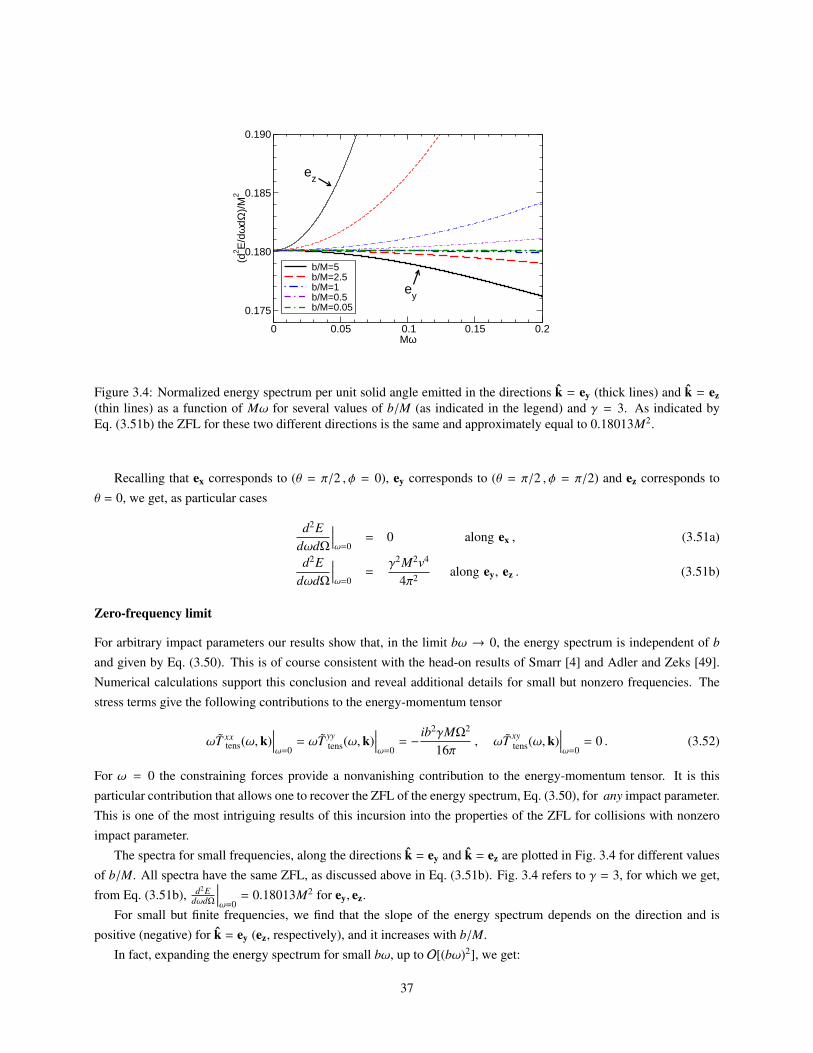
0 0.05 0.1 0.15 0.2Mω

0.175

0.180

0.185

0.190

(d2 E

/dω

dΩ)/

M2

b/M=5b/M=2.5b/M=1b/M=0.5b/M=0.05

ey

ez

Figure 3.4: Normalized energy spectrum per unit solid angle emitted in the directions k = ey (thick lines) and k = ez(thin lines) as a function of Mω for several values of b/M (as indicated in the legend) and γ = 3. As indicated byEq. (3.51b) the ZFL for these two different directions is the same and approximately equal to 0.18013M2.

Recalling that ex corresponds to (θ = π/2 , φ = 0), ey corresponds to (θ = π/2 , φ = π/2) and ez corresponds toθ = 0, we get, as particular cases

d2EdωdΩ

∣∣∣∣ω=0

= 0 along ex , (3.51a)

d2EdωdΩ

∣∣∣∣ω=0

=γ2M2v4

4π2 along ey, ez . (3.51b)

Zero-frequency limit

For arbitrary impact parameters our results show that, in the limit bω → 0, the energy spectrum is independent of b

and given by Eq. (3.50). This is of course consistent with the head-on results of Smarr [4] and Adler and Zeks [49].Numerical calculations support this conclusion and reveal additional details for small but nonzero frequencies. Thestress terms give the following contributions to the energy-momentum tensor

ωT xxtens(ω,k)

∣∣∣∣ω=0

= ωT yytens(ω,k)

∣∣∣∣ω=0

= −ib2γMΩ2

16π, ωT xy

tens(ω,k)∣∣∣∣ω=0

= 0 . (3.52)

For ω = 0 the constraining forces provide a nonvanishing contribution to the energy-momentum tensor. It is thisparticular contribution that allows one to recover the ZFL of the energy spectrum, Eq. (3.50), for any impact parameter.This is one of the most intriguing results of this incursion into the properties of the ZFL for collisions with nonzeroimpact parameter.

The spectra for small frequencies, along the directions k = ey and k = ez are plotted in Fig. 3.4 for different valuesof b/M. All spectra have the same ZFL, as discussed above in Eq. (3.51b). Fig. 3.4 refers to γ = 3, for which we get,from Eq. (3.51b), d2E

dωdΩ

∣∣∣∣ω=0

= 0.18013M2 for ey, ez.For small but finite frequencies, we find that the slope of the energy spectrum depends on the direction and is

positive (negative) for k = ey (ez, respectively), and it increases with b/M.In fact, expanding the energy spectrum for small bω, up to O[(bω)2], we get:

37

d2EdωdΩ

=γ2M2v2

16π2(1 − v2 sin2 θ cos2 φ

)2

4v2(sin2 θ cos2 φ − 1)2 −

−16

[v2

(8v2 + 3

)sin6 θ cos4 φ + sin2 θ

((8v2 + 3

)cos 2φ + 12

(v2 + 1

))−

− sin4 θ cos2 φ(6v4 +

(2v2 + 3

)v2 cos 2φ + 20v2 + 3

)− 12

][bω]2

+ O

[(bω)3

]. (3.53)

Thus, within our model the spectrum typically has quadratic corrections, except along k = ex, for which the firstnonvanishing contribution to the energy spectrum is of order (bω)4. In fact, we find

d2EdωdΩ

∣∣∣∣∣k=ex

= −γ2M2

(3 − 2v2

)2

9216π2 (bω)4 + O[(bω)5

]. (3.54)

This small frequencies behaviour can be seen in Fig. (3.4).

Extreme mass ratio collisions

We now study collisions for µ ≡ M1 M2 ≡ M. The energy spectrum can be computed in the center-of-momentumframe. Since particle 2 is much heavier than particle 1, the former is practically at rest in this frame, although we shallnot neglect the motion of this particle when we compute the energy-momentum tensor. Therefore, we let v ≡ v1 v2

and γ ≡ γ1.From Eqs. (3.33) and (3.39), the angular frequency and position of particle 1 are given by

Ω =γ1µv1ξ1 + γ2Mv2ξ2

γ1µξ1 + γ2Mξ2, ξ1 =

bγ2Mγ1µ + γ2M

. (3.55)

Once again we must add the stresses needed to constrain the particles in their orbits, in order to have a conservedenergy-momentum tensor.

Radiation spectrum

The radiated energy is computed using Eq. (1.52) or Eq. (1.54). Once again the Jacobi-Anger expansion (3.47) andEq. (3.49) are used to compute the Fourier transforms. We expand the energy-momentum tensor in powers of µ/M, andcompute the energy keeping only leading-order contributions in µ/M. A calculation of the energy for γ = 3 in severaldifferent directions yields the spectra shown in Fig. 3.5.

The extreme-mass ratio configuration loses the angular symmetry of the equal mass case. Therefore, the spectranow diverge for all multiples of Ω for k = ex, k = ey. The behaviour is similar for other directions. This was also foundin Sec. 2.2. For k = ez, the spectrum only diverges for ω = 2Ω, in agreement with Poisson’s findings for particles incircular orbit around black holes [60].

Head-on collisions

For extreme-mass ratio head-on collisions (b = 0) we find

d2EdωdΩ

=γ2µ2v4

(sin2 θ cos2 φ − 1

)2

4π2(v sin θ cos φ − 1)2 . (3.56)

This expression coincides, as it should, with Eq. (3.16).For ease of comparison with numerical and perturbative results of point particles in black hole spacetimes (see Sec. 3.3),in Appendix B we perform a multipole decomposition of this ZFL result in spin-weighted spherical harmonics.

38

0 0.2 0.4 0.6 0.8 1 1.2 1.4 1.6 1.8 2ω/Ω

10-4

10-3

10-2

10-1

100

101

102

103

104

(d2 E

/dω

dΩ)/

µ2

(ex+ey+21/2

ez)/2exeyez

Figure 3.5: Normalized energy spectrum per solid angle emitted in the directions k = ex, ey, ez, (ex + ey +√

2ez)/2 asa function of ω/Ω in the extreme mass ratio case.

Zero-frequency limit

Let us now consider the ZFL for generic values of the impact parameter. As bω → 0 we find once again that theenergy spectrum is independent of the impact parameter (as it was for the equal-mass collisions of section 3.2). Theleading-order expression of the energy in powers of µ/M is given by Eq. (3.56), reproducing Smarr’s result for head-oncollisions. Including higher powers of bω we get

d2EdωdΩ

=γ2µ2v2

4π2(v sin θ cos φ − 1)2

v2(sin2 θ cos2 φ − 1)2 −

−1

192

[(−4v

(2v2 + 3

)sin3 θ(cos 2θ + 3) cos 3φ + 8 sin2 θ cos 2φ

((3 − 10v2

)cos 2θ − 6v2 + 9

)+

+ v sin θ cos φ((

372 − 8v2)

cos 2θ +(6v2 + 9

)cos 4θ + 2v2 + 387

)+ 8

(2v2 − 21

)cos 2θ +

+(20v2 − 6

)cos 4θ − 6

(6v2 + 35

) ][bω]2

+ O

[(bω)3

]. (3.57)

As in the equal-mass case, here too the radiation is suppressed along the x–axis, where the leading contribution isof order (bω)4

d2EdωdΩ

∣∣∣∣∣k=ex

=γ2µ2(3 − 2v(v + 3))2

576π2 [bω]4 + O[(bω)5

]. (3.58)

Generic mass ratio

The same procedure can be used to study a collision between two particles of arbitrary masses. We compute theradiated energy, once again in the center-of-momentum frame, for two particles colliding, for γ1 = 3 and M1 = M2/3.The Fourier transforms are once again computed using the Jacobi-Anger expansion and summing only from −10 to10. In Fig. 3.6 we show the radiated energy per unit frequency per solid angle emitted in several directions. As we cansee, similarly to the extreme mass ratio case, all spectra diverge for all multiples of the rotating frequency. The onlyexception remains k = ez, where the spectrum only diverges at twice the rotating frequency, as discussed above.Taking the ω → 0 limit we recover, once again, the energy obtained by Smarr for the head-on collision, given byEq. (3.13) (Smarr’s Eq. (2.16)).

39

0 0.2 0.4 0.6 0.8 1 1.2 1.4 1.6 1.8 2ω/Ω

10-4

10-3

10-2

10-1

100

101

102

103

104

(dE

/dω

dΩ)/

(GM

12 )

(ex+ey+21/2

ez)/2exeyez

Figure 3.6: Normalized energy per solid angle and per unit frequency emitted in the directions k = ex, ey, ez, (ex + ey +√

2ez)/2 as a function of ω/Ω for mass ratio q = M1/M2 = 1/3 and γ1 = 3. The zero frequency limit agrees withSmarr’s energy [Eq. (2.16)] for a head-on collision with unequal mass.

Generality of the model

The most important result of our ZFL calculation for collisions with generic impact parameter is perhaps that the ZFLitself is independent of the impact parameter. One of the limitations of the present calculation is that the modellingof the collision is rather ad-hoc, especially in the specification of the nature of the constraining forces. It is natural toask how the results would change if the constraining forces were modelled differently. For example, in our toy modelthe final system consists of two particles bound in a circular orbit, so the radiation spectrum shows peaks typical of theradiation produced by rotating bodies. There is a chance that the divergence at harmonics of the rotational frequencyof the final system could contaminate the low-frequency behaviour of the spectrum.

To investigate this possibility, instead of considering the collision of two point particles, we studied a point particlecolliding with a special extended matter distribution: specifically, we considered an infinitely thin, slowly rotating,uniform disk. For brevity we do not report details of this calculation here. Our main finding is that, if the disk isinitially slowly rotating (so that after the collision the system is at rest), the ZFL is the same as in the case of twocolliding particles. This is by no means a proof that the ZFL is completely independent of the way one models thesystem. It is however a hint that (as physical intuition would suggest) the ZFL should only depend on the asymptoticmomenta of the colliding particles.

3.3 High Energy Collision of Black Holes

The high energy collision of two black holes is one of the most violent process one can have in general relativity.The absence of analytical solutions leaves many unanswered questions about what happens in such collisions. Thesecollisions provide a test to the cosmic censorship conjecture, is it possible to form a naked singularity, or will an eventhorizon always be formed?Moreover, the interest in ultrarelativistic collisions increased with the proposal that the Planck scale could be as lowas a TeV (thus solving the hierarchy problem) in higher dimensional scenarios, either with large extra dimensions [61]or with compact dimensions with large warp factor [62]. Lowering the Planck scale opens the possibility of black

40

hole production in particle colliders and ultra high energy cosmic ray interactions with the atmosphere (for a reviewsee [63]). Therefore computing the radiated energy in such processes, as well as the production cross section has agrowing interest.Finally, the AdS/CFT correspondence conjecture [64] further motivates the study of these high-speed black hole colli-sions. This duality could be used to understand properties of the quark-gluon plasma formed in gold ion collisions atBrookhaven’s Relativist Heavy Ion Collider, by studying black hole collisions in AdS [65].

There have been several attempts to understand these ultrarelativistic black hole collisions, by various approaches.A comparison of the techniques described bellow can be found in Ref. [66]. In the seventies Penrose [67] studied theproblem of a classical collision with zero impact parameter. Penrose modelled the spacetime as the superposition oftwo Aichelburg-Sexl waves7. When the two shock waves collide, they interact nonlinearly, and a closed trapped surfaceis formed. By finding this closed trapped surface Penrose was able to set a lower bound on the mass of the final hole of√

s/2, where√

s is the center-of-momentum energy. Later D’Eath and Payne [69, 70, 71] refined this calculation andfound an estimate of 0.84

√s for the mass of the final hole. However this energy was obtained by computing the first

two terms of a series expansions of the news functions, and it does not include the radiation emitted during the decayof the final black hole to equilibrium (Schwarzschild). This construction was expanded to non head-on collisions inarbitrary dimensions by Eardley and Giddings [72], and a numerical investigation of their equations was performedin [73, 74].

Another method to compute the radiated energy is to use a perturbation theory approach, considering a small pointparticle falling into a large black hole. The background metric is taken to be that of the black hole, and the metric per-turbation hµν is induced by the point particle. The Einstein equations can then be expanded to the first order in hµν, andthe problem is expressed as a second order differential equation for the metric perturbation. This method was first usedto study the head-on collision of two bodies in 1971 in [21], using the Zerilli equation for black hole perturbations [20].The authors considered a small test particle falling radially, from rest at infinity, into a Schwarzschild black hole. Thesecalculations were also extended to the case of infall from finite radius [75]. Later Ruffini generalized these results for aparticle falling with an initial velocity [26]. These results were then extended to a massless particle falling from infinitythrough a radial geodesic [76], thus extending the previous results for large boost factors. The extension of these resultsfor a spherically-symmetric black hole in D dimensions was also carried out in Ref. [77]. The gravitational radiationfor generic orbits of particles falling, from rest at infinity, into a Kerr black hole was studied by Sasaki, Nakamura andcollaborators in [78]. These calculations were then extended for a highly relativistic point particle falling into a Kerrblack hole, using the Sasaki-Nakamura formalism in [79, 80]. This method should only hold as long as the particle’senergy E is much smaller than the black hole’s mass MBH . However these results can be extrapolated for energiesE ∼ MBH and still give sensible results [76, 79, 80]. The Post-Newtonian approximation also provides a way to studythese collisions. The radiated energy in the head-on collision of two bodies of arbitrary masses, starting from rest, iscomputed in [81]. The authors of [81] then compare the Post-Newtonian results with those obtained using perturbationtheory.

Another approach was explored by Smarr in 1977 [4], where he used the Zero Frequency Limit approximation tocompute the gravitational radiation emitted during the head-on collisions and scattering of black holes, modelled aspoint particles. Although the total energy depends on a parameter not fixed by the theory, this method provides an es-timate of the energy radiated per unit frequency, its polarization and angular distribution. This approach is in excellent

7The Aichelburg-Sexl metric [68] corresponds to the Schwarzschild metric boosted, and taking the limit of large boost and small mass, keepingthe total energy fixed.

41

agreement with the perturbative calculations described above [76, 77, 79, 80]. Since this method requires a linearizedapproximation, it would not be expected to hold for the high-energy collision of two black holes, as pointed out inthe previous Sections, which should in principle require the inclusion of nonlinear effects. Surprisingly this methodstill describes quite well even the nonlinear ultrarelativistic head-on collision of black holes [83]. We now comparethe ZFL approximation with perturbative calculations and numerical results, which justifies our interest in such anapproximation, providing an additional motivation to the ZFL extension for non head-on collisions, carried out in theprevious Section.

Let us consider the extreme mass ratio black hole collision described in Sec. 3.1. For such collisions Smarr proposedthat the cutoff frequency ωc could be the inverse of the large black hole radius ωc ∼ r−1

H , where rH = 2M. As we willsee, this cutoff actually corresponds to a “weighted average” of the lowest damped quasi-normal modes.Taking the limit v→ 1 in Eq, (3.16), so that these results can be compared against the perturbative results found in [76]for a ultrarelativistic test particle falling into a Schwarzschild black hole we get

dEZFL

dω=

43πγ2 µ

2

M∼ 0.4244γ2 µ

2

M. (3.59)

Cardoso and Lemos [76] found the radiated energy at zero frequency to be

dEdω

∣∣∣∣∣ω=0

= 0.4244γ2 µ2

M, (3.60)

which is in excellent agreement with the ZFL method. If we now integrate Smarr’s result up to ωc ∼ r−1H to have an

estimate for the total radiated energy, we get Smarr’s Eq. (3.5)

∆EZFL ∼ 0.2γ2 µ2

M. (3.61)

However this seems to underestimate the total radiated energy, as shown in [76], where the authors found

∆E ∼ 0.262γ2 µ2

M, (3.62)

which equivalent to set the cutoff frequency at ωc ∼ (1.63M)−1. For comparison with the perturbative calculations itis convenient to expand this results in spin-weight −2 spherical harmonics, as described in Appendix B. The multipolecontent of the radiated energy is then given by

dEl0

dω=

4γ2µ2

π

(2l + 1)(l − 2)!(l + 2)!

, (3.63)

where only the m = 0 modes contribute. The perturbative results are in agreement with this calculation, as the spec-tra is flat up to a certain cutoff, decaying rapidly to zero afterwards. The cutoff is well approximated by the lowestquasinormal mode, for each l. Therefore the cutoff frequency should be given by some “weighted average” of the fun-damental gravitational quasinormal modes frequencies, similarly to what was found when considering the gravitationalscattering in Sec. 3.1.The authors also found in Refs. [79, 80] that the radiated energy at zero frequency has the same value independently ofthe spin of the large black hole, and for particles falling along the equator [79] or along the symmetry axis [80].For a head-on collision in higher dimensional spacetimes, Eq.(3.20) is, once again, in agreement with the perturbativeapproach, as shown in [77], where the authors considered a perturbed Schwarzschild-Tangherlini black hole, by anultrarelativistic point particle falling radially into the black hole.

42

Figure 3.7: Numerical results for the normalized energy spectrum for the l = 2, m = 0 mode, for several β = v. Takenfrom Ref. [83].

For non head-on collisions the perturbative approximation carried out in Ref. [1], for a point particle falling intoa Schwarzschild black hole, shows that the zero frequency limit of the radiation spectrum is weakly dependant onthe impact parameter, and in quite good agreement with the ZFL prediction (particularly for larger boost factors). Inaddition Eq. B.13 predicts that, in the ZFL, the ratio between the l = 2 ,m = 2 mode and the l = 2 ,m = 0 mode is 3/2,which is in very good agreement with the perturbative results.The radiated momentum for an extreme mass ratio collision computed in Sec. 3.1 is also in agreement with the pertur-bative calculations of Ref. [1] for the zero frequency limit of head-on collisions.

So far we have only described analytical methods, which provide estimates and bounds for the radiated energy.We now address the numerical study of these collisions, which is the only way to study black hole collisions withthe full nonlinear Einstein equations. The numerical simulation of a black hole collision has been studied for long[22, 82, 83, 84, 85]. What is remarkable is that the simulations of highly boosted head-on black hole collisions is stillin reasonable agreement with the ZFL results [83]. Sperhake et al. [83] found that, even though the spectrum is nolonger flat for small frequencies, it is nearly flat up to a some cutoff frequency, which is well approximated by theleast-damped quasinormal mode of the final hole. After the cutoff frequency the spectrum decays exponentially. Thiscan be seen in Fig. 3.7, which is Fig. 2 of Ref. [83]. The l = 2, m = 0 component of the radiated energy is plottedas a function of Mω, where M denotes the mass of the final black hole, for several values of β = v. Note that theauthors considered the collision along the z-axis, so only the m = 0 modes contribute. The straight lines correspond tothe ZFL projected into spherical spin-weight harmonics (see Appendix B), and the vertical lines to the least-dampedquasinormal mode l = 2.

43

Appendix A

Spherical Coordinates in (D − 1)−dimensions

In Chapters 2 and 3 spherical coordinates in (D−1)−dimensions were considered, when studying gravitational radiationin higher dimensional spacetimes. Here we briefly review some important results. We introduce spherical coordinates(r, θ1, . . . , θD−2), which are related to the Cartesian coordinates (x1, . . . , xD−1) by 1

x1 = r sin θ1 sin θ2 . . . sin θD−2

x2 = r sin θ1 sin θ2 . . . sin θD−3 cos θD−2...

xi = r sin θ1 sin θ2 . . . sin θD−i−1 cos θD−i...

xD−1 = r cos θ1

.

This means that the volume element becomes dD−1x = rD−2drdΩD−2, where dΩD−2 = sinD−3 θ1 sinD−4 θ2 . . . sin θD−3dθ1

. . . dθD−2 is the element of the solid angle. Integration over the angle variables yields ΩD−2 = 2π(D−1)/2

Γ[(D−1)/2] . Here, andthroughout Chapters 2 and 3, we have used that∫ π

0sinn θ =

√π

Γ[(n + 1)/2]Γ[(n + 2)/2]

. (A.1)

A.1 Useful Integrals

In Chapters 1, 2 and 3 we used some integrals of the projector Λi j,kl (Eq. (2.17)) times a certain number of ni, over thesolid angle, which we list here. ∫

dΩD−2 = ΩD−2 (A.2)∫dΩD−2 ni . . . nk︸ ︷︷ ︸

odd number

= 0 (A.3)∫dΩD−2nin j =

ΩD−2

D − 1δi j (A.4)∫

dΩD−2nin jnknl =ΩD−2

D2 − 1

(δi jδkl + δikδ jl + δilδ jk

)(A.5)∫

dΩD−2nin jnknlnmno =ΩD−2

(D2 − 1)(D + 3)

(δi jδklδmo + . . .

), (A.6)

where the . . . in the final expression denotes all possible pairings.

1When using spherical coordinates in D = 4 we have that φ = π/2 − θ/2.

45

Appendix B

Multipolar Decomposition of the Radiated Energy

When considering the radiated gravitational energy in Chapter 3 we performed a multipolar decomposition of theradiated energy, in order to compare the ZFL calculations against known numerical and perturbative results. Multipolarexpansions are widely used to study gravitational radiation (see [86] for a review). In numerical relativity it is commonto expand in the Newman-Penrose spin-weighted spherical harmonics (SWSH) [87]. In this appendix we review theSWSH, and consider the decomposition of the radiated energy.

B.1 Spin-weighted Spherical Harmonics

Let us consider an orthonormal reference frame X1, X2, X3 such that X1 and X2 are tangent to a sphere with radiusr, and X3 is normal to that sphere. Such a frame is defined up to rotations about X3. If we define X = 1

√2(X1 + iX2)

these rotations can be written as X′ = eiχX. We say that a quantity has spin s if it transforms as η′ = eisχη under theserotations. We now choose the frame to be X1 = 1

r∂∂θ

, X2 = 1r sin θ

∂∂φ

, X3 = ∂∂r . Let us define the operator ð, acting on a

quantity η of spin s, as

ðη = − (sin θ)s(∂

∂θ+

isin θ

∂

∂φ

)(sin θ)−s η , (B.1)

which has spin 1 under rotations.

The spin-weight s spherical harmonics sYlm are then defined by acting with ð on the usual spherical harmonics Ylm

sYlm =

√

(l−s)!(l+s)!ð

sYlm , 0 6 s 6 l√(l+s)!(l−s)!ð

s∗Ylm , −l 6 s 6 0,

where the star denotes complex conjugation. Note that the SWSH are not defined for |s| < l. One also the followingproperties

sYlm = (−1)m+s−sYl−m , sYlm(π − θ, φ + φ) = (−1)l

−sYl−m(θ, φ) . (B.2)

The spin-weight spherical harmonics form a complete orthonormal set for each value of s, which means one can expandany quantity of spin s in this basis. The spin-weight |s| = 2 is of interest to gravitational radiation [87], and can beobtained from the spin 0 spherical harmonics by

2Ylm =

√(l − 2)!(l + 2)!

(∂2θ − cot θ∂θ +

m2

sin2 θ−

2msin θ

(∂θ − cot θ))

Ylm . (B.3)

47

The usual spherical harmonics Ylm can be determined from the Legendre polynomials Plm(x)

Ylm(θ, φ) =

√2l + 1

4π(l − m)!(l + m)!

Plm(cos θ)eimφ . (B.4)

B.2 Decomposition of the Radiated Energy

In numerical relativity it is common to expand the Weyl scalar Ψ4 in spin-weight −2 spherical harmonics. The Weyltensor is defined as the Riemann tensor with all of its contractions removed Cρσµν = Rρσµν + 1

3 gρ[µgν]σR − gρ[µRν]σ +

gσ[µRν]ρ, where the square brackets denote antisymmetrization. The contractions of the Weyl tensor with members ofthe null tetrad are denoted by Ψ0 , . . . ,Ψ4. As discussed in Sec. 1.2, if we consider a gravitational wave travelling alonga direction denoted by n, we can define the “plus” and “cross” polarizations. Let us consider an orthonormal frameX1, X2, X3, with X3 = n. Then the metric perturbation in this frame defines the “plus” and “cross” components of themetric h+ = hTT

11 = −hTT22 , h× = hTT

12 , where the indexes 1, 2 refer to the frame considered. The Weyl scalar Ψ4 is thengiven by Ψ4 = 1

2

(h+ − ih×

), which is expanded in spin-weight −2 spherical harmonics. The energy radiated through a

sphere at infinity, given by Eq. (1.48), can be written in terms of h+ and h× as

d2EdtdΩ

=r2

16π

⟨|h+|

2 + |h×|2⟩

av. (B.5)

Let us consider the Fourier transform of the radiated energy, which can be written in terms of the Weyl scalar Ψ4 by

d2EdtdΩ

=r2

4πω2

⟨|Ψ4|

2⟩

av. (B.6)

This means that the radiated energy can also be expanded in spin-weight spherical harmonics in the following way

d2EdtdΩ

=

∑lm

√dElm

dt −2Ylm

2

, (B.7)

where√

dElmdt are yet undetermined functions of t. These functions can be computed using the orthonormality of −2Ylm

by √dElm

dt=

∫dΩ

√d2EdtdΩ

−2Ylm . (B.8)

We can now determine the multipolar decomposition of the radiated energy in a head-on collision (Sec. 3.1).Before proceeding, we must go back to the angles chosen in Sec. 3.1, where we considered the collision to be alongthe x axis. If we had considered a collision along the z axis instead, (as in Refs. [4, 49]) there would be no dependenceon the azimuthal angle φ, and the calculations when decomposing the energy would be greatly simplified. In whatfollows we consider the collision to be along the z axis to find the multipolar decomposition of the radiated energyfor ultrarelativistic collisions. After obtaining the multipolar decomposition of the energy, a rotation can be performedto change the collision back to the x axis. The multipolar components in a rotated frame can be found following theprocedure discussed in Ref. [88].

Equal mass collisions

The radiated energy, for an ultrarelativistic (v → 1) equal mass collision along the x axis is (see Eq. (3.14) and thechange of angles discussed above the equation)

d2EdωdΩ

=m2γ2

1

π2 . (B.9)

48

Since there is no φ dependence only the m = 0 modes contribute, and we find

dEl0

dω=

16γ2m2

π(2l+1)(l−2)!

(l+2)! , l even

0 , l odd,

where we have used Eqs. (B.3) and(B.4). We see that the l = 2 mode is the one which contributes most, since for largel the energy is suppressed by a factor of 1/l3. Summing over even l we find dE

dω = 4γ2m2/π, which is in agreement withEq. (3.15) in the v→ 1 limit.

Extreme mass ratio collisions

For an ultrarelativistic, extreme mass ratio collision, along the z axis we find from Eq. (3.16) (changing the angles asdiscussed above)

d2EdωdΩ

=γ2

1µ2 (1 + cos θ)2

4π2 . (B.10)

Once again the independence on φ means that only the m = 0 modes contribute, and we find

dEl0

dω=

4γ2µ2

π

(2l + 1)(l − 2)!(l + 2)!

. (B.11)

Summing over l we get dEdω = 4γ2m2/(3π), which is in agreement with Eq. (3.17), in the v→ 1 limit.

Rotation

The two frames considered, one where the collision takes place along the z axis, and the other where it takes placealong the x axis, are related by a rotation of π/2 about the y axis. As shown above, for a collision along the z axis theindependence of the φ angle means that only the m = 0 contribute. However when we rotate back into the previousframe this is not the case. The transformation of the multipolar decomposition of the radiated energy under rotations isexplained in Ref. [88]. The multipolar components, for this rotation, transform as follows√

dElm

dω=

√dEl0

dωA(l)

m0 , (B.12)

where we have used the fact that only the m = 0 modes contribute, and the matrix A(l)mm′ can be found in Ref. [88]. Let

us consider the l = 2 modes, which are the dominant ones, for the extreme mass ratio collision, in the v→ 1 limit. Themultipolar components of the radiated energy in the rotated frame (where the collision takes place along x) is

dEl±2

dω=

516

γ2µ2

π,

dEl0

dω=

524

γ2µ2

π, (B.13)

with the m = ±1 modes vanishing. For an equal mass collision, in the same limit, we have that the m = ±1 vanish, andthat

dEl±2

dω=

54γ2m2

π, l even

0 , l odd,

dEl0

dω=

56γ2m2

π, l even

0 , l odd.

For arbitrary velocities one finds for the dominant mode, l = 2, and for m = 0

dE20

dω=

5m2γ2(−10v3 + 3

γ4 log(

2v+1 − 1

)+ 6v

)2

96πv6 , (B.14)

where the rotation has already been performed, such that the collision takes place along the x axis. Similarly for anextreme mass ratio collision we have that

dE20

dω=

5m2γ2(v(5v2 − 3

)+ 3

γ4 tanh−1(v))2

96πv6 . (B.15)

49

Bibliography

[1] E. Berti, V. Cardoso, T. Hinderer, M. Lemos, F. Pretorius, U. Sperhake and N. Yunes, arXiv:1003.0812 [gr-qc].

[2] V. Cardoso, M. Lemos, and M. Marques, Phys. Rev. D 80 (2009) 127502 [arXiv:1001.0019 [gr-qc]].

[3] W. H. Press, Phys. Rev. D 15 (1977) 965.

[4] L. Smarr, Phys. Rev. D 15, 2069 (1977).

[5] S. Weinberg, “Gravitation and Cosmology,” Wiley, New York (1972).

[6] C. W. Misner, K. S. Thorne and J. A. Wheeler, “Gravitation,” San Francisco (1973), 1279p.

[7] S. M. Carroll, “Spacetime and geometry: An introduction to general relativity,” San Francisco, USA: Addison-

Wesley (2004) 513p.

[8] M. Maggiore, “Gravitational Waves. Vol. 1: Theory and Experiments,” Oxford University Press, (2007) 572p.

(ISBN-13: 978-0-19-857074-5)

[9] R. d’Inverno, “Introducing Einstein’s relativity,” Oxford, UK: Clarendon (1992) 383p.

[10] V. Cardoso, O. J. C. Dias and J. P. S. Lemos, Phys. Rev. D 67 (2003) 064026 [arXiv:hep-th/0212168].

[11] W. Kinnersley and M. Walker, Phys. Rev. D 2 (1970) 1359.

[12] S. Hassani, “Mathematical Physics,” Springer-Verlag, New York (1998).

[13] A. Einstein, Preuss. Akad. Wiss. Berlin, Sitzber (1918) 154 as cited in [86]

[14] R. A. Isaacson, Phys. Rev. 166 (1968) 1272.

[15] K. S. Thorne, S. J. Kovacs, Astrophys. J. 200 (1975) 245 .

[16] W. B. Bonnor, M. A. Rotenberg, Proc. Roy. Soc. A265 (1961) 109.

[17] A. Peres, Phys. Rev. 128 (1962) 2471. ; A. Papapetrou, Compt. Rend. 255 (1962) 1578. ; W. B. Bonnor, M. A.Rotenberg, Proc. Roy. Soc. A289 (1966) 247. ; F. I. Cooperstock, Phys. Rev. 165 (1968) 1424

[18] J. D. Bekenstein, Astrophys. J. 183 (1973) 657.

[19] D. D. Dionysiou, J. Phys. A 10 (1977) 969.

[20] F. J. Zerilli, Phys. Rev. D 2 (1970) 2141.

[21] M. Davis, R. Ruffini, W. H. Press and R. H. Price, Phys. Rev. Lett. 27, 1466 (1971).

51

[22] S. G. Hahn and R. W. Lindquist, Ann. Phys. 29, 304 (1964). L. Smarr, “The Structure of General Relativitywith a Numerical Illustration: The Collision of Two Black Holes”, Univ. of Texas at Austin Ph.D. Thesis (1975)as cited in [82] ; K.R. Eppley, Princeton Ph.D. Thesis (1977) as cited in [82] ; P. Anninos, D. Hobill, E. Seidel,L. Smarr and W. M. Suen, Phys. Rev. Lett. 71 (1993) 2851 [arXiv:gr-qc/9309016]. ; P. Anninos, D. Hobill,E. Seidel, L. Smarr and W. M. Suen, Phys. Rev. D 52 (1995) 2044 [arXiv:gr-qc/9408041]. ; J. G. Baker,A. Abrahams, P. Anninos, S. Brandt, R. Price, J. Pullin and E. Seidel, Phys. Rev. D 55 (1997) 829 [arXiv:gr-qc/9608064]. ; P. Anninos and S. Brandt, Phys. Rev. Lett. 81 (1998) 508 [arXiv:gr-qc/9806031].

[23] S. L. Smarr (ed.), “Sources of Gravitational Radiation,” Cambridge University Press (1979).

[24] R. Ruffini and J. A. Wheeler, in “Proceedings of the Cortona Symposium on Weak Interactions”, edited byL. Radicati, Accademia Nazionale Dei Lincei, Rome (1971) as cited in [21].

[25] T. Regge and J. A. Wheeler, Phys. Rev. 108 (1957) 1063.

[26] R. Ruffini, Phys. Rev. D 7 (1973) 972.

[27] M. J. Fitchett, The Gravitational Recoil Effect and its Astrophysical Consequences, (PhD Thesis, University ofCambridge, 1984).

[28] F. R. Tangherlini, Nuovo Cim. 27 (1963) 636.

[29] T. Nakamura and M. P. Haugan, Astrophys. J. 269 (1983) 292.

[30] E. Balbinski, S. Detweiler, L. Lindblom and B. Schutz, Mon. Not. Roy. Astron. Soc. 213 (1985) 553.

[31] P. C. Peters and J. Mathews, Phys. Rev. 131 (1963) 435.

[32] R. A. Hulse, J. H. Taylor, Astrophys. J. Lett. 195 (1975) L51.

[33] J. H. Taylor and J. M. Weisberg, Astrophys. J. 253 (1982) 908. ; J. M. Weisberg and J. H. Taylor, Phys. Rev.Lett. 52 (1984) 1348 ; J. H. Taylor and J. M. Weisberg, Astrophys. J. 345 (1989) 434. ; J. M. Weisberg andJ. H. Taylor, arXiv:astro-ph/0211217. ;

[34] J. M. Weisberg and J. H. Taylor, ASP Conf. Ser. 328 (2005) 25 [arXiv:astro-ph/0407149].

[35] M. J. Fitchett, Mon. Not. Roy. Astron. Soc. 203 (1983) 1049.

[36] M. J. Fitchett and S. Detweiler, Mon. Not. Roy. Astron. Soc. 211 (1984) 933 .

[37] P. C. Peters, Phys. Rev. 136 (1964) B1224.

[38] E. Poisson, Living Rev. Rel. 7 (2004) 6. URL (cited on 21 May 2009): http://www.livingreviews.org/lrr-2004-6[arXiv:gr-qc/0306052].

[39] S. A. Hughes, arXiv:0903.4877 [astro-ph.CO].

[40] J. A. Gonzalez, U. Sperhake, B. Bruegmann, M. Hannam and S. Husa, Phys. Rev. Lett. 98 (2007) 091101[arXiv:gr-qc/0610154].

[41] J. A. Gonzalez, M. D. Hannam, U. Sperhake, B. Bruegmann and S. Husa, Phys. Rev. Lett. 98 (2007) 231101[arXiv:gr-qc/0702052].

52

[42] M. Campanelli, C. O. Lousto, Y. Zlochower and D. Merritt, Phys. Rev. Lett. 98 (2007) 231102 [arXiv:gr-qc/0702133].

[43] J. D. Jackson, “Classical Electrodynamics, third edition,” J. Wiley, New York (1999).

[44] L. D. Landau, E. M. Lifshitz, “The Classical theory of fields, fourth revised English edition” Butterworth-

Heinemann (1980)

[45] J. A. Wheeler, “Geometrodynamics,” Academic, New York (1962).

[46] R. P. Feynman, letter to V. F. Weisskopf (1961), unpublished, as cited in [4]

[47] S. Weinberg, Phys. Lett. 9 (1964) 357 ; S. Weinberg, Phys. Rev. 135 (1964) B1049. ; S. Weinberg, Phys. Rev.140 (1965) B516. ; S. Weinberg, Phys. Rev. 134 (1964) B882.

[48] B. S. DeWitt, Phys. Rev. 160 (1967) 1113. ; B. S. DeWitt, Phys. Rev. 162 (1967) 1195. ; B. S. DeWitt, Phys.Rev. 162 (1967) 1239.

[49] R. J. Adler and B. Zeks, Phys. Rev. D 12 (1975) 3007.

[50] P. N. Payne, Phys. Rev. D 28 (1983) 1894.

[51] A. P. Lightman, W. H. Press, R. H. Price and S. A. Teukolsky, “Problem Book in Relativity and Gravitation”Princeton Univ. Press, Princeton (1975).

[52] P. C. Peters, Phys. Rev. D 1 (1970) 1559.

[53] M. Turner, and C. M. Will Astrophys. J. 220 (1978) 1107.

[54] S. J. Kovacs and K. S. Thorne, Astrophys. J. 217 (1977) 252.

[55] S. J. Kovacs and K. S. Thorne, Astrophys. J. 224 (1978) 62.

[56] R. Ruffini and J. A. Wheeler, in “The Significance of Space Research for Fundamental Physics,” edited byA. F. Moore and V. Hardy European Space Research Organization, Paris (1971). as cited in [55]

[57] P. C. Peters, Phys. Rev. D 5 (1972) 2476.

[58] R. H. Price and V. D. Sandberg, Phys. Rev. D 8, 1640 (1973).

[59] M. Abramowitz and I. A. Stegun “Handbook of Mathematical Functions with Formulas, Graphs, and Mathe-matical Tables,” Dover, New York (1972).

[60] E. Poisson, Phys. Rev. D 47, 1497 (1993).

[61] N. Arkani-Hamed, S. Dimopoulos and G. R. Dvali, Phys. Lett. B 429 (1998) 263 [arXiv:hep-ph/9803315]. ;I. Antoniadis, N. Arkani-Hamed, S. Dimopoulos and G. R. Dvali, Phys. Lett. B 436 (1998) 257 [arXiv:hep-ph/9804398].

[62] L. Randall and R. Sundrum, Phys. Rev. Lett. 83 (1999) 3370 [arXiv:hep-ph/9905221]. ; L. Randall and R. Sun-drum, Phys. Rev. Lett. 83 (1999) 4690 [arXiv:hep-th/9906064].

[63] S. B. Giddings, in Proc. of the APS/DPF/DPB Summer Study on the Future of Particle Physics (Snowmass

2001) ed. N. Graf, (2001) pp P328 [arXiv:hep-ph/0110127].

53

[64] J. M. Maldacena, Adv. Theor. Math. Phys. 2 (1998) 231 [Int. J. Theor. Phys. 38 (1999) 1113] [arXiv:hep-th/9711200]. ; E. Witten, Adv. Theor. Math. Phys. 2 (1998) 253 [arXiv:hep-th/9802150]. ; S. S. Gubser,I. R. Klebanov and A. M. Polyakov, Phys. Lett. B 428 (1998) 105 [arXiv:hep-th/9802109].

[65] H. Nastase, arXiv:hep-th/0501068. ; S. S. Gubser, S. S. Pufu and A. Yarom, Phys. Rev. D 78 (2008) 066014[arXiv:0805.1551 [hep-th]]. ; A. J. Amsel, D. Marolf and A. Virmani, JHEP 0804 (2008) 025 [arXiv:0712.2221[hep-th]].

[66] V. Cardoso, E. Berti and M. Cavaglia, Class. Quant. Grav. 22 (2005) L61 [arXiv:hep-ph/0505125].

[67] R. Penrose, presented at the Cambrisge University Seminar, Cambridge, England, 1974 (unpublished, as citedin [69]).

[68] P. C. Aichelburg and R. U. Sexl, Gen. Rel. Grav. 2 (1971) 303.

[69] P. D. D’Eath and P. N. Payne, Phys. Rev. D 46, 658 (1992). ; P. D. D’Eath and P. N. Payne, Phys. Rev. D 46,675 (1992). ; P. D. D’Eath and P. N. Payne, Phys. Rev. D 46, 694 (1992).

[70] P. D. D’Eath, Phys. Rev. D 18, 990 (1978).

[71] P. D. D’Eath, “Black holes: Gravitational interactions,” Oxford, UK: Clarendon (1996) 286 p. (Oxford mathe-

matical monographs)

[72] D. M. Eardley and S. B. Giddings, Phys. Rev. D 66, 044011 (2002) [arXiv:gr-qc/0201034].

[73] H. Yoshino and Y. Nambu, Phys. Rev. D 67 (2003) 024009 [arXiv:gr-qc/0209003].

[74] H. Yoshino and V. S. Rychkov, Phys. Rev. D 71 (2005) 104028 [Erratum-ibid. D 77 (2008) 089905] [arXiv:hep-th/0503171].

[75] C. O. Lousto and R. H. Price, Phys. Rev. D 55 (1997) 2124 [arXiv:gr-qc/9609012].

[76] V. Cardoso and J. P. S. Lemos, Phys. Lett. B 538 (2002) 1 [arXiv:gr-qc/0202019].

[77] E. Berti, M. Cavaglia and L. Gualtieri, Phys. Rev. D 69 (2004) 124011 [arXiv:hep-th/0309203].

[78] Y. Kojima and T. Nakamura, Prog. Theor. Phys. 71 (1984) 79. ; M. Sasaki and T. Nakamura, Prog. Theor. Phys.67 (1982) 1788. ; T. Nakamura and M. Sasaki, Phys. Lett. A 89 (1982) 185. ; Y. Kojima and T. Nakamura, Phys.Lett. A 96 (1983) 335. ; Y. Kojima and T. Nakamura, Phys. Lett. A 99 (1983) 37.

[79] V. Cardoso and J. P. S. Lemos, Phys. Rev. D 67 (2003) 084005 [arXiv:gr-qc/0211094].

[80] V. Cardoso and J. P. S. Lemos, Gen. Rel. Grav. 35 (2003) 327 [arXiv:gr-qc/0207009].

[81] L. E. Simone, E. Poisson and C. M. Will, Phys. Rev. D 52 (1995) 4481 [arXiv:gr-qc/9506080].

[82] F. Pretorius, arXiv:0710.1338 [gr-qc].

[83] U. Sperhake, V. Cardoso, F. Pretorius, E. Berti and J. A. Gonzalez, Phys. Rev. Lett. 101 (2008) 161101[arXiv:0806.1738 [gr-qc]].

[84] M. Shibata, H. Okawa and T. Yamamoto, Phys. Rev. D 78 (2008) 101501 [arXiv:0810.4735 [gr-qc]].

54

[85] U. Sperhake, V. Cardoso, F. Pretorius, E. Berti, T. Hinderer and N. Yunes, Phys. Rev. Lett. 103 (2009) 131102[arXiv:0907.1252 [gr-qc]].

[86] K. S. Thorne, Rev. Mod. Phys. 52 (1980) 299.

[87] E. T. Newman and R. Penrose, J. Math. Phys. 7 (1966) 863. ; J. N. Goldberg, A. J. MacFarlane, E. T. Newman,F. Rohrlich and E. C. G. Sudarshan, J. Math. Phys. 8 (1967) 2155. ; E. T. Newman and R. Penrose, Proc. Roy.Soc. Lond. A 305 (1968) 175.

[88] L. Gualtieri, E. Berti, V. Cardoso and U. Sperhake, Phys. Rev. D 78 (2008) 044024 [arXiv:0805.1017 [gr-qc]].

55