APPROXIMATION METHODS

Kenneth L. Judd

Hoover Institution

July 17, 2012

Approximation Methods

I General Objective: Given data about f (x) construct simpler g(x) toapproximate f (x).

I Questions:I What data should be produced and used?I What family of “simpler” functions should be used?I What notion of approximation do we use?

I Comparisons with statistical regressionI Both approximate an unknown function and use a finite amount of

dataI Statistical data is noisy but we assume data errors are smallI Nature produces data for statistical analysis but we produce the data

in function approximation

Interpolation Methods

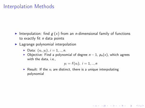
I Interpolation: find g (x) from an n-dimensional family of functionsto exactly fit n data points

I Lagrange polynomial interpolationI Data: (xi , yi ) , i = 1, .., n.I Objective: Find a polynomial of degree n − 1, pn(x), which agrees

with the data, i.e.,yi = f (xi ), i = 1, .., n

I Result: If the xi are distinct, there is a unique interpolatingpolynomial

I Does pn(x) converge to f (x) as we use more points?I No! Consider

f (x) =1

1+ x2

xi = −5,−4, ..., 3, 4, 5

• Does pn(x) converge to f (x) as we use more points?

— No! Consider

f(x)=1

1 + x2xi=−5,−4, ..., 3, 4, 5

Figure 1:

— Why does this fail? because there are zero degrees of freedom? bad choice of points? bad

function?

4

I Why does this fail? because there are zero degrees of freedom? badchoice of points? bad function?

I Hermite polynomial interpolationI Data: (xi , yi , y ′i ) , i = 1, .., n.I Objective: Find a polynomial of degree 2n − 1, p(x), which agrees

with the data, i.e.,

yi = p(xi ), i = 1, .., n

y ′i = p′(xi ), i = 1, .., n

I Result: If the xi are distinct, there is a unique interpolatingpolynomial

I Least squares approximationI Data: A function, f (x).I Objective: Find a function g(x) from a class G that best

approximates f (x), i.e.,

g = arg ming∈G‖f − g‖2

Orthogonal polynomials

I General orthogonal polynomialsI Space: polynomials over domain DI Weighting function: w(x) > 0I Inner product: 〈f , g〉 =

´D f (x)g(x)w(x)dx

I Definition: {φi} is a family of orthogonal polynomials w.r.t w (x) iff

〈φi , φj 〉 = 0, i 6= j

I We can compute orthogonal polynomials using recurrence formulas

φ0(x) = 1

φ1(x) = x

φk+1(x) = (ak+1x + bk)φk(x) + ck+1φk−1(x)

I Chebyshev polynomialsI [a, b] = [−1, 1] and w(x) =

(1− x2)−1/2

I Tn(x) = cos(n cos−1 x)I Recursive definition

T0(x) = 1T1(x) = xTn+1(x) = 2x Tn(x)− Tn−1(x),

I Graphs

• Chebyshev polynomials

— [a, b] = [−1, 1] and w(x) =(1− x2

)−1/2

— Tn(x) = cos(n cos−1 x)

— Recursive definitionT0(x) = 1

T1(x) = x

Tn+1(x) = 2xTn(x)− Tn−1(x),

— Graphs

7

I General intervalsI Few problems have the specific intervals and weights used in

definitionsI One must adapt the polynomials to fit the domain through linear

COV:I Define the linear change of variables that maps the compact interval

[a, b] to [−1, 1]

y = −1 + 2x − ab − a

I The polynomials φ∗i (x) ≡ φi

(−1 + 2 x−a

b−a

)are orthogonal over

x ∈ [a, b] with respect to the weight w∗ (x) ≡(−1 + 2 x−a

b−a

)iff the

φi (y) are orthogonal over y ∈ [−1, 1] w.r.t. w (y)

Regression

I Data: (xi , yi ) , i = 1, .., n.I Objective: Find a function f (x ;β) with β ∈ Rm, m ≤ n, with

yi.= f (xi ), i = 1, .., n.

I Least Squares regression:

minβ∈Rm

∑(yi − f (xi ;β))

2

Algorithm 6.4: Chebyshev Approximation Algorithm in R1

I Objective: Given f (x) on [a, b], find Chebyshev poly approx p(x)I Step 1: Define m ≥ n + 1 Chebyshev interpolation nodes on [−1, 1]:

zk = −cos(2k − 12m

π

), k = 1, · · · ,m.

I Step 2: Adjust nodes to [a, b] interval:

xk = (zk + 1)(

b − a2

)+ a, k = 1, ...,m.

I Step 3: Evaluate f at approximation nodes:

wk = f (xk) , k = 1, · · · ,m.I Step 4: Compute Chebyshev coefficients, ai , i = 0, · · · , n :

ai =

∑mk=1 wkTi (zk)∑mk=1 Ti (zk)2

p(x) =n∑

i=0

aiTi

(2x − ab − a

− 1)

Minmax ApproximationI Data: (xi , yi ) , i = 1, .., n.I Objective: L∞ fit

minβ∈Rm

maxi‖yi − f (xi ;β)‖

I Problem: Difficult to computeI Chebyshev minmax property

Suppose f : [−1, 1]→ R is C k for some k ≥ 1, and let In be the degree npolynomial interpolation of f based at the zeroes of Tn+1(x). Then

‖ f − In ‖∞≤(2π

log(n + 1) + 1)

× (n − k)!n!

(π2

)k(

b − a2

)k

‖ f (k) ‖∞

I Chebyshev interpolation:I converges in L∞; essentially achieves minmax approximationI works even for C 2 and C 3 functionsI easy to computeI does not necessarily approximate f ′ well

Shape Issues

I Approximation methods and shapeI Concave (monotone) data may lead to nonconcave (nonmonotone)

approximations.I Shape problems destabilize value function iteration

Shape Issues

• Approximation methods and shape

— Concave (monotone) data may lead to nonconcave (nonmonotone) approximations.

— Example

— Shape problems destabilize value function iteration

14

Shape-preserving polynomial approximation

I Least squares Chebyshev approximation that preserves increasingconcave shape with Lagrange data (xi , vi )

mincj

m∑i=1

n∑j=0

cjφj (xi )− vi

2

s.t.n∑

j=1

cjφ′j (xi ) > 0,

n∑j=1

cjφ′′j (xi ) < 0, i = 1, . . . ,m.

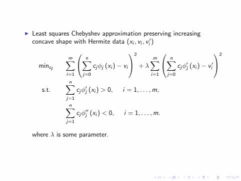
I Least squares Chebyshev approximation preserving increasingconcave shape with Hermite data (xi , vi , v ′i )

mincj

m∑i=1

n∑j=0

cjφj (xi )− vi

2

+ λ

m∑i=1

n∑j=0

cjφ′j (xi )− v ′i

2

s.t.n∑

j=1

cjφ′j (xi ) > 0, i = 1, . . . ,m,

n∑j=1

cjφ′′j (xi ) < 0, i = 1, . . . ,m.

where λ is some parameter.

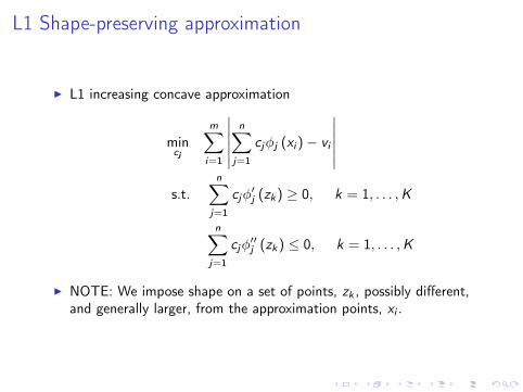
L1 Shape-preserving approximation

I L1 increasing concave approximation

mincj

m∑i=1

∣∣∣∣∣∣n∑

j=1

cjφj (xi )− vi

∣∣∣∣∣∣s.t.

n∑j=1

cjφ′j (zk) ≥ 0, k = 1, . . . ,K

n∑j=1

cjφ′′j (zk) ≤ 0, k = 1, . . . ,K

I NOTE: We impose shape on a set of points, zk , possibly different,and generally larger, from the approximation points, xi .

I This looks like a nondifferentiable problem, but it is not when werewrite it as

mincj ,λi

m∑i=1

λi

s.t.n∑

j=1

cjφ′j (zk) ≥ 0, k = 1, . . . ,K

n∑j=1

cjφ′′j (zk) ≤ 0, k = 1, . . . ,K

−λi ≤n∑

j=1

cjφj (xi )− vi ≤ λi , i = 1, . . . ,m

0 ≤ λi , i = 1, . . . ,m

I Use possibly different points for shape constraints; generally youwant more shape checking points than data points.

I Mathematical justification: semi-infinite programmingI Many other procedures exist for one-dimensional problems, but few

procedures exist for two-dimensional problems

Multidimensional approximation methods

I Lagrange InterpolationI Data: D ≡ {(xi , zi )}Ni=1 ⊂ Rn+m, where xi ∈ Rn and zi ∈ Rm

I Objective: find f : Rn → Rm such that zi = f (xi ).I Need to choose nodes carefully.I Task: Find combinations of interpolation nodes and spanning

functions to produce a nonsingular (well-conditioned) interpolationmatrix.

Tensor products

I General Approach:I If A and B are sets of functions over x ∈ Rn, y ∈ Rm, their tensor

product isA⊗ B = {ϕ(x)ψ(y) | ϕ ∈ A, ψ ∈ B}.

I Given a basis for functions of xi , Φi = {ϕik(xi )}∞k=0, the n-fold tensor

product basis for functions of (x1, x2, . . . , xn) is

Φ =

{n∏

i=1

ϕiki (xi ) | ki = 0, 1, · · · , i = 1, . . . , n

}

I Orthogonal polynomials and Least-square approximationI Suppose Φi are orthogonal with respect to wi (xi ) over [ai , bi ]I Least squares approximation of f (x1, · · · , xn) in Φ is∑

ϕ∈Φ

〈ϕ, f 〉〈ϕ,ϕ〉 ϕ,

where the product weighting function

W (x1, x2, · · · , xn) =n∏

i=1

wi (xi )

defines 〈·, ·〉 over D =∏

i [ai , bi ] in

〈f (x), g(x)〉 =

ˆD

f (x)g(x)W (x)dx .

Algorithm 6.4: Chebyshev Approximation Algorithm in R2

I Objective: Given f (x , y) defined on [a, b]× [c , d ], find its Chebyshevpolynomial approximation p(x , y)

zk = −cos(2k − 12m

π

), k = 1, · · · ,m.

xk = (zk + 1)(

b − a2

)+ a, k = 1, ...,m.

yk = (zk + 1)(

d − c2

)+ c , k = 1, ...,m.

wk,` = f (xk , y`) , k = 1, · · · ,m. , ` = 1, · · · ,m.

p(x , y) =n∑

i=0

n∑j=0

aijTi

(2x − ab − a

− 1)

Tj

(2y − cd − c

− 1)

Polynomials

I Taylor’s theorem for Rn produces the approximation

f (x) .= f (x0) +∑n

i=1∂f∂xi

(x0) (xi − x0i )

+ 12

∑ni1=1

∑ni2=1

∂2f∂xi1∂xik

(x0)(xi1 − x0i1)(xik − x0

ik) + ...

I For k = 1, Taylor’s theorem for n dimensions used the linearfunctions Pn

1 ≡ {1, x1, x2, · · · , xn}I For k = 2, Taylor’s theorem usesPn

2 ≡ Pn1 ∪ {x2

1 , · · · , x2n , x1x2, x1x3, · · · , xn−1xn}.

I In general, the kth degree expansion uses the complete set ofpolynomials of total degree k in n variables.

Pnk ≡ {x

i11 · · · x

inn |

n∑`=1

i` ≤ k, 0 ≤ i1, · · · , in}

I Complete orthogonal basis includes only terms with total degree k orless.

I Sizes of alternative bases

degree k Pnk Tensor Prod.

2 1+ n + n(n + 1)/2 3n

3 1+ n + n(n+1)2 + n2 + n(n−1)(n−2)

6 4n

I Complete polynomial bases contains fewer elements than tensorproducts.

I Asymptotically, complete polynomial bases are as good as tensorproducts.

I For smooth n-dimensional functions, complete polynomials are moreefficient approximations

I ConstructionI Compute tensor product approximation, as in Algorithm 6.4I Drop terms not in complete polynomial basis (or, just compute

coefficients for polynomials in complete basis).I Complete polynomial version is faster to compute since it involves

fewer termsI Almost as accurate as tensor product; in general, degree k + 1

complete is better then degree k tensor product but uses far fewerterms.

Shape Issues

I Much harder in higher dimensionsI No general methodI The L2 and L1 methods generalize to higher dimensions.

I The constraints will be restrictions on directional derivatives in manydirections

I There will be many constraintsI But, these will be linear constraintsI L1 reduces to linear programming; we can now solve huge LP

problems, so don’t worry.