Embed Size (px)
Citation preview
Approximation of functions of large matrices.
Part I. Computational aspects
V. Simoncini
Dipartimento di Matematica, Universita di Bologna
and CIRSA, Ravenna, Italy
1
The problem
Given A ∈ Rn×n, v ∈ R
n and f sufficiently smooth function,
approximate
x = f(A)v
⋆ A large dimension, ‖v‖ = 1
⋆ A sym. pos. (semi)def., or A positive real
⋆ f(A)v vs f(A)
Projection-type methods
K approximation space, m = dim(K) V ∈ Rn×m s.t. K = range(V )
x = f(A)v ≈ xm = V f(V ⊤AV )(V ⊤v)
2
The problem
Given A ∈ Rn×n, v ∈ R
n and f sufficiently smooth function,
approximate
x = f(A)v
⋆ A large dimension, ‖v‖ = 1
⋆ A sym. pos. (semi)def., or A positive real
⋆ f(A)v vs f(A)
Projection-type methods
K approximation space, m = dim(K) V ∈ Rn×m s.t. K = range(V )
x = f(A)v ≈ xm = V f(V ⊤AV )(V ⊤v)
3
Numerical approximation.
f(A)v ≈ x
Important issues:
⋆ Role of f in the approximation quality
⋆ Role of A in the approximation quality
⋆ Efficiency ?
⋆ Measures/Estimates of accuracy?
4
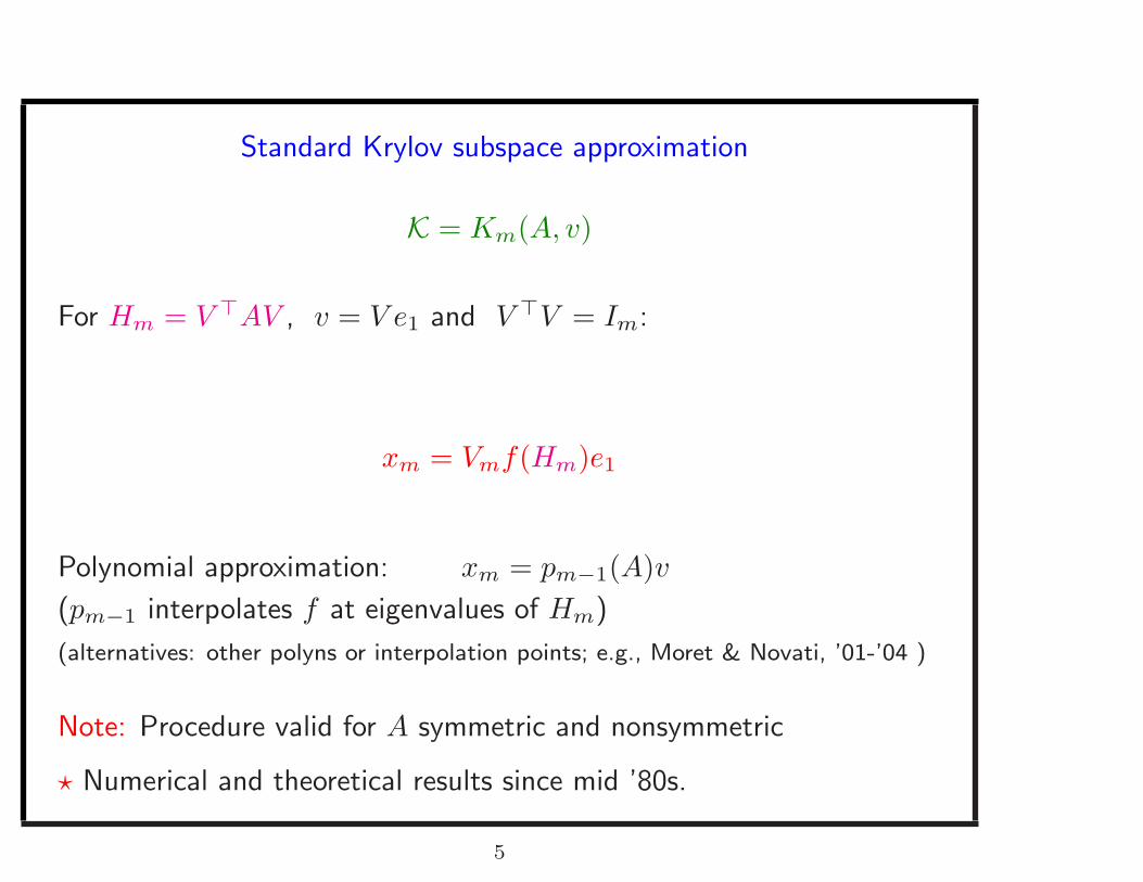
Standard Krylov subspace approximation
K = Km(A, v)
For Hm = V ⊤AV , v = V e1 and V ⊤V = Im:
xm = Vmf(Hm)e1
Polynomial approximation: xm = pm−1(A)v
(pm−1 interpolates f at eigenvalues of Hm)
(alternatives: other polyns or interpolation points; e.g., Moret & Novati, ’01-’04 )
Note: Procedure valid for A symmetric and nonsymmetric
⋆ Numerical and theoretical results since mid ’80s.
5
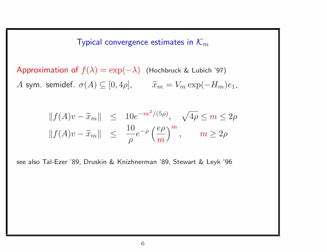
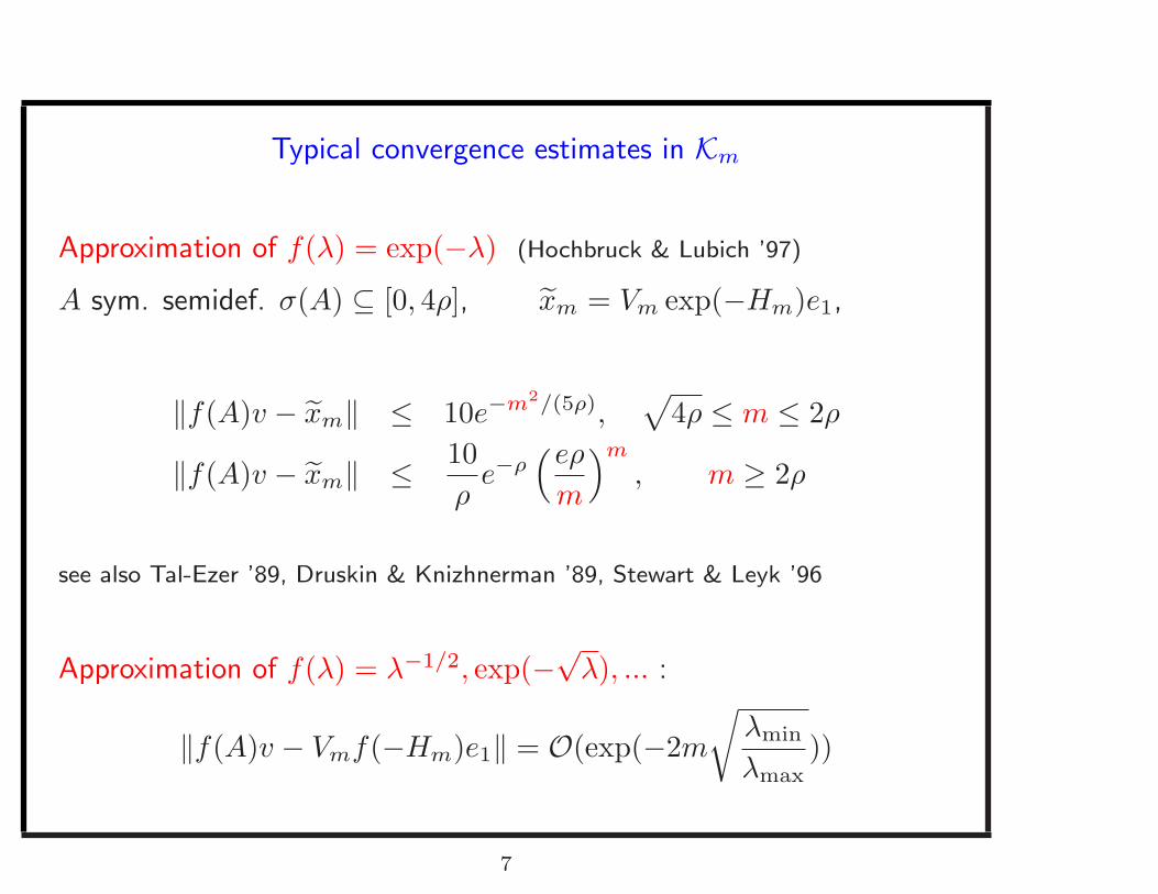
Typical convergence estimates in Km
Approximation of f(λ) = exp(−λ) (Hochbruck & Lubich ’97)
A sym. semidef. σ(A) ⊆ [0, 4ρ], xm = Vm exp(−Hm)e1,
‖f(A)v − xm‖ ≤ 10e−m2/(5ρ),√
4ρ ≤ m ≤ 2ρ
‖f(A)v − xm‖ ≤ 10
ρe−ρ
(eρ
m
)m
, m ≥ 2ρ
see also Tal-Ezer ’89, Druskin & Knizhnerman ’89, Stewart & Leyk ’96
Approximation of f(λ) = λ−1/2, exp(−√
λ), ... :
‖f(A)v − Vmf(−Hm)e1‖ = O(exp(−2m
√λmin
λmax))
6
Typical convergence estimates in Km
Approximation of f(λ) = exp(−λ) (Hochbruck & Lubich ’97)
A sym. semidef. σ(A) ⊆ [0, 4ρ], xm = Vm exp(−Hm)e1,
‖f(A)v − xm‖ ≤ 10e−m2/(5ρ),√
4ρ ≤ m ≤ 2ρ
‖f(A)v − xm‖ ≤ 10
ρe−ρ
(eρ
m
)m
, m ≥ 2ρ
see also Tal-Ezer ’89, Druskin & Knizhnerman ’89, Stewart & Leyk ’96
Approximation of f(λ) = λ−1/2, exp(−√
λ), ... :
‖f(A)v − Vmf(−Hm)e1‖ = O(exp(−2m
√λmin
λmax))
7
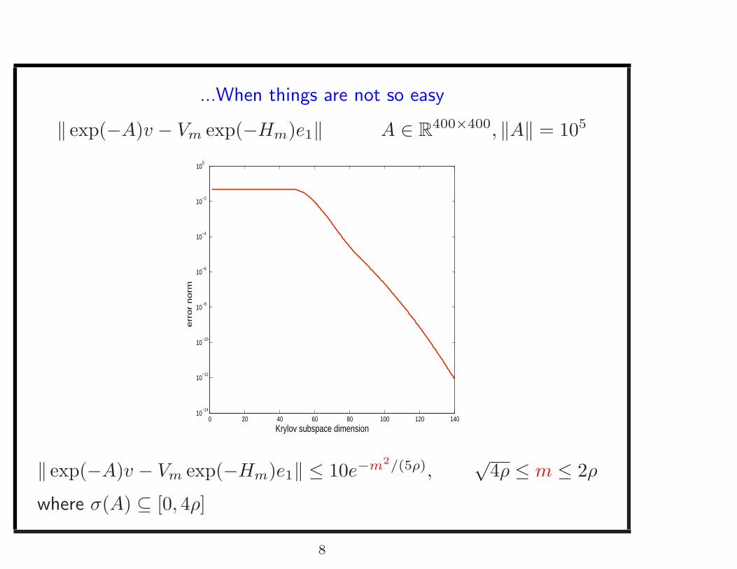
...When things are not so easy
‖ exp(−A)v − Vm exp(−Hm)e1‖ A ∈ R400×400, ‖A‖ = 105
0 20 40 60 80 100 120 14010
−14
10−12
10−10
10−8
10−6
10−4
10−2
100
Krylov subspace dimension
err
or
no
rm
‖ exp(−A)v − Vm exp(−Hm)e1‖ ≤ 10e−m2/(5ρ),√
4ρ ≤ m ≤ 2ρ
where σ(A) ⊆ [0, 4ρ]
8
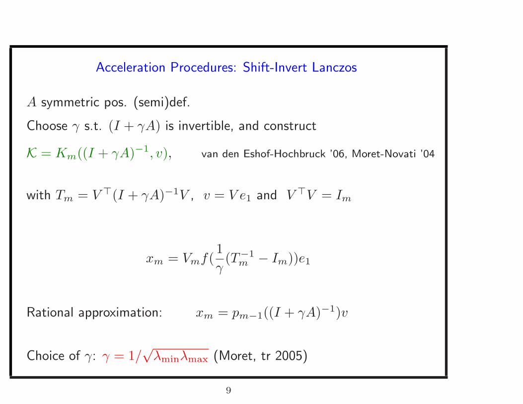
Acceleration Procedures: Shift-Invert Lanczos
A symmetric pos. (semi)def.
Choose γ s.t. (I + γA) is invertible, and construct
K = Km((I + γA)−1, v), van den Eshof-Hochbruck ’06, Moret-Novati ’04
with Tm = V ⊤(I + γA)−1V , v = V e1 and V ⊤V = Im
xm = Vmf(1
γ(T−1
m − Im))e1
Rational approximation: xm = pm−1((I + γA)−1)v
Choice of γ: γ = 1/√
λminλmax (Moret, tr 2005)
9
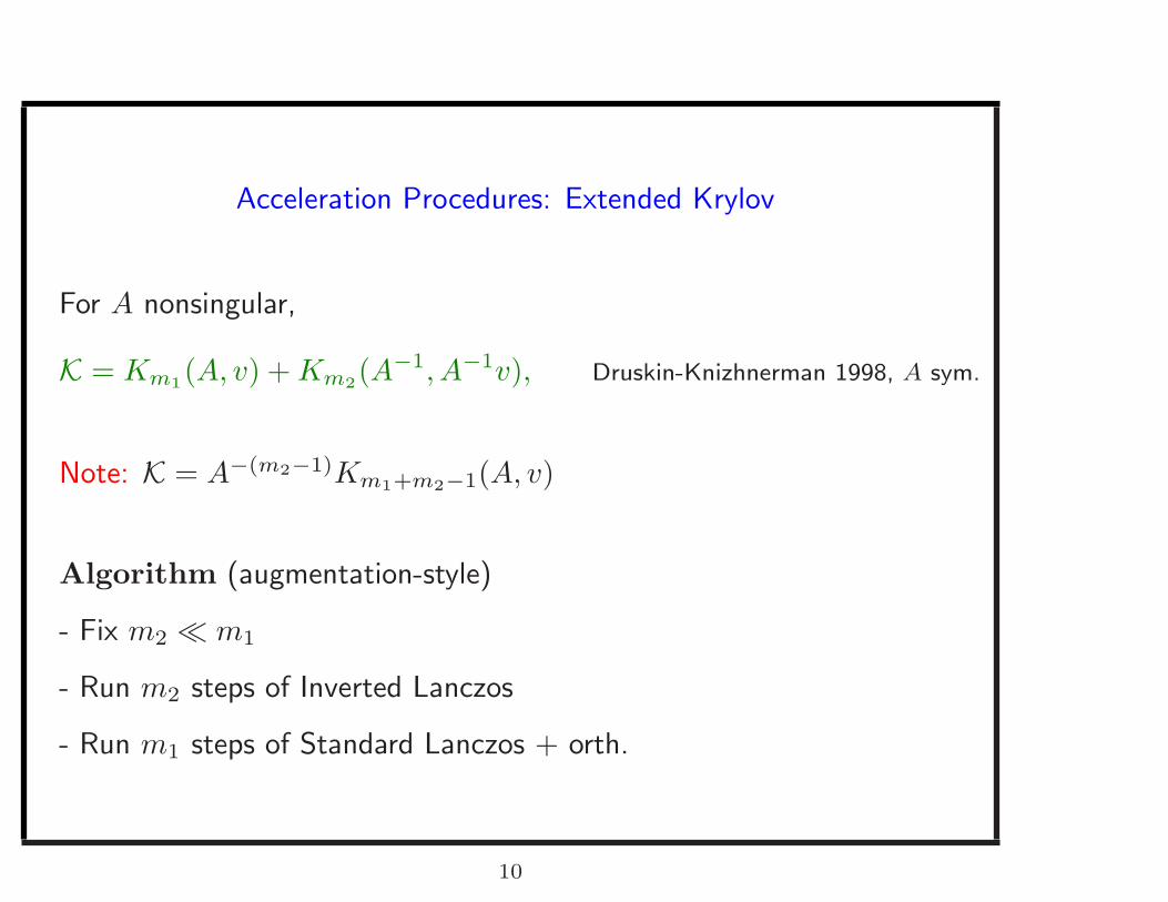
Acceleration Procedures: Extended Krylov
For A nonsingular,
K = Km1(A, v) + Km2
(A−1, A−1v), Druskin-Knizhnerman 1998, A sym.
Note: K = A−(m2−1)Km1+m2−1(A, v)
Algorithm (augmentation-style)
- Fix m2 ≪ m1
- Run m2 steps of Inverted Lanczos
- Run m1 steps of Standard Lanczos + orth.
10
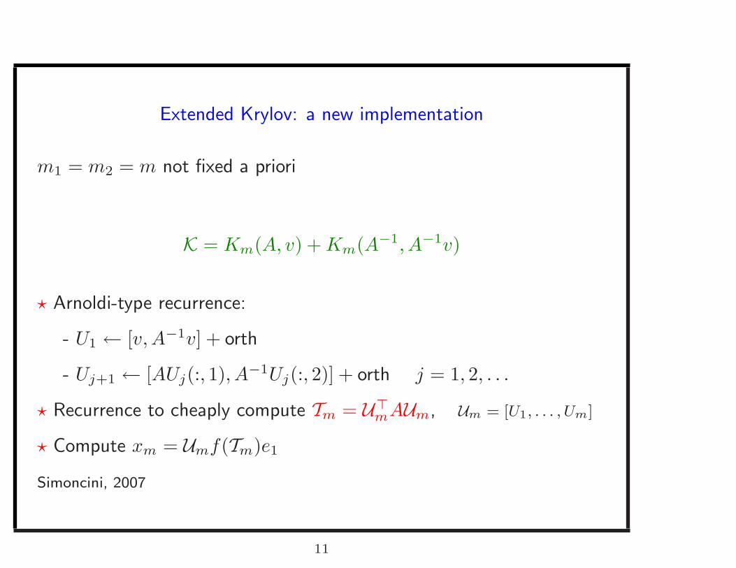
Extended Krylov: a new implementation
m1 = m2 = m not fixed a priori
K = Km(A, v) + Km(A−1, A−1v)
⋆ Arnoldi-type recurrence:
- U1 ← [v, A−1v] + orth
- Uj+1 ← [AUj(:, 1), A−1Uj(:, 2)] + orth j = 1, 2, . . .
⋆ Recurrence to cheaply compute Tm = U⊤mAUm, Um = [U1, . . . , Um]
⋆ Compute xm = Umf(Tm)e1
Simoncini, 2007
11
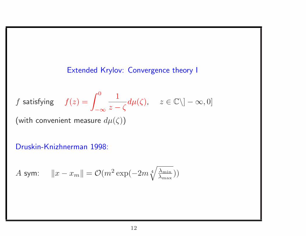
Extended Krylov: Convergence theory I
f satisfying f(z) =
∫ 0
−∞
1
z − ζdµ(ζ), z ∈ C\] −∞, 0]
(with convenient measure dµ(ζ))
Druskin-Knizhnerman 1998:
A sym: ‖x − xm‖ = O(m2 exp(−2m 4
√λmin
λmax
))
12
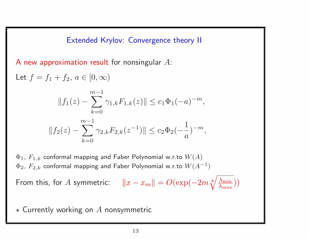
Extended Krylov: Convergence theory II
A new approximation result for nonsingular A:
Let f = f1 + f2, a ∈ [0,∞)
‖f1(z) −m−1∑
k=0
γ1,kF1,k(z)‖ ≤ c1Φ1(−a)−m,
‖f2(z) −m−1∑
k=0
γ2,kF2,k(z−1)‖ ≤ c2Φ2(−1
a)−m,
Φ1, F1,k conformal mapping and Faber Polynomial w.r.to W (A)
Φ2, F2,k conformal mapping and Faber Polynomial w.r.to W (A−1)
From this, for A symmetric: ‖x − xm‖ = O(exp(−2m 4
√λmin
λmax
))
⋆ Currently working on A nonsymmetric
13
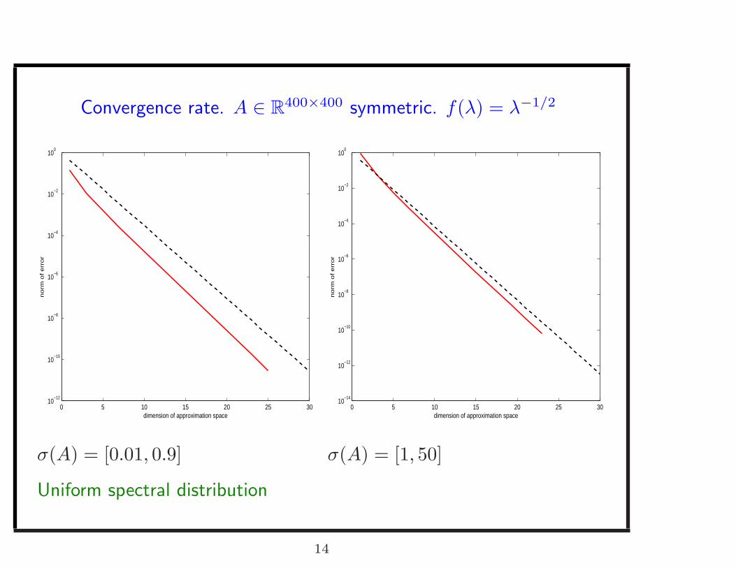
Convergence rate. A ∈ R400×400 symmetric. f(λ) = λ−1/2
0 5 10 15 20 25 3010
−12
10−10
10−8
10−6
10−4
10−2
100
dimension of approximation space
no
rm o
f e
rro
r
σ(A) = [0.01, 0.9]
0 5 10 15 20 25 3010
−14
10−12
10−10
10−8
10−6
10−4
10−2
100
dimension of approximation space
no
rm o
f e
rro
r
σ(A) = [1, 50]
Uniform spectral distribution
14
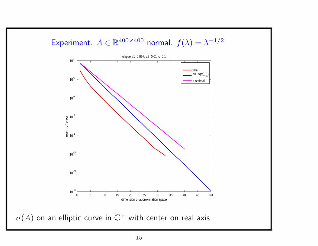
Experiment. A ∈ R400×400 normal. f(λ) = λ−1/2
0 5 10 15 20 25 30 35 40 45 5010
−14
10−12
10−10
10−8
10−6
10−4
10−2
100
dimension of approximation space
no
rm o
f e
rro
r
ellipse a1=0.097, a2=0.01, c=0.1
true a=−sqrt(l
1ln)
a optimal
σ(A) on an elliptic curve in C+ with center on real axis
15
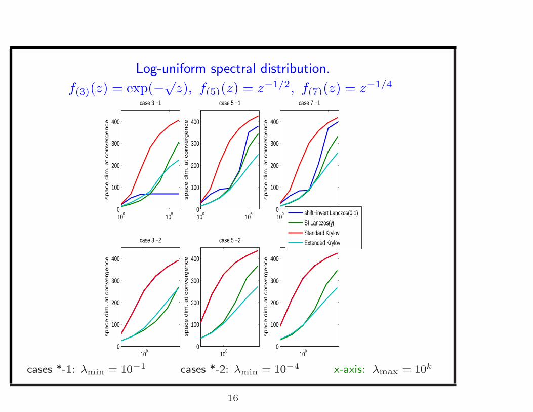
Log-uniform spectral distribution.
f(3)(z) = exp(−√z), f(5)(z) = z−1/2, f(7)(z) = z−1/4
100
105
0
100
200
300
400
sp
ace
dim
. a
t co
nve
rge
nce
case 3 −1
100
0
100
200
300
400
sp
ace
dim
. a
t co
nve
rge
nce
case 3 −2
100
105
0
100
200
300
400
sp
ace
dim
. a
t co
nve
rge
nce
case 5 −1
100
0
100
200
300
400
sp
ace
dim
. a
t co
nve
rge
nce
case 5 −2
100
105
0
100
200
300
400
sp
ace
dim
. a
t co
nve
rge
nce
case 7 −1
100
0
100
200
300
400sp
ace
dim
. a
t co
nve
rge
nce
case 7 −2
shift−invert Lanczos(0.1)
SI Lanczos(γ)Standard Krylov
Extended Krylov
cases *-1: λmin = 10−1 cases *-2: λmin = 10−4 x-axis: λmax = 10k
16
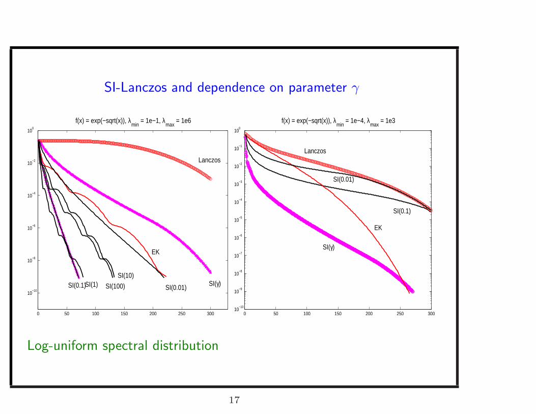
SI-Lanczos and dependence on parameter γ
0 50 100 150 200 250 300
10−10
10−8
10−6
10−4
10−2
100
f(x) = exp(−sqrt(x)), λmin
= 1e−1, λmax
= 1e6
SI(0.1)SI(1) SI(100)
SI(10)
EK
SI(γ)
Lanczos
SI(0.01)
0 50 100 150 200 250 30010
−10
10−9
10−8
10−7
10−6
10−5
10−4
10−3
10−2
10−1
100
f(x) = exp(−sqrt(x)), λmin
= 1e−4, λmax
= 1e3
SI(0.01)
SI(0.1)
SI(γ)
Lanczos
EK
Log-uniform spectral distribution
17
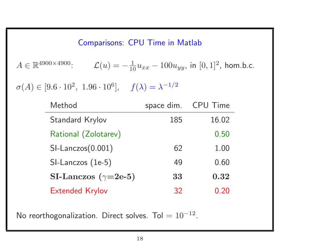
Comparisons: CPU Time in Matlab
A ∈ R4900×4900: L(u) = − 1
10uxx − 100uyy, in [0, 1]2, hom.b.c.
σ(A) ∈ [9.6 · 102, 1.96 · 106], f(λ) = λ−1/2
Method space dim. CPU Time
Standard Krylov 185 16.02
Rational (Zolotarev) 0.50
SI-Lanczos(0.001) 62 1.00
SI-Lanczos (1e-5) 49 0.60
SI-Lanczos (γ=2e-5) 33 0.32
Extended Krylov 32 0.20
No reorthogonalization. Direct solves. Tol = 10−12.
18
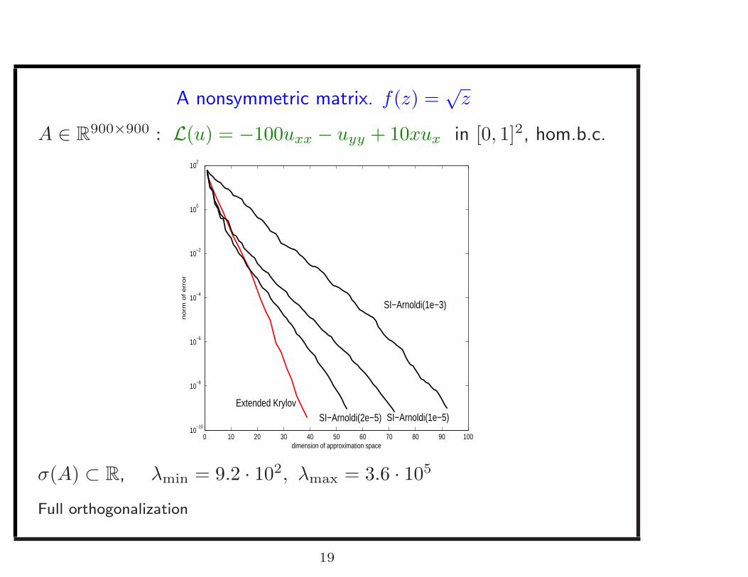
A nonsymmetric matrix. f(z) =√
z
A ∈ R900×900 : L(u) = −100uxx − uyy + 10xux in [0, 1]2, hom.b.c.
0 10 20 30 40 50 60 70 80 90 10010
−10
10−8
10−6
10−4
10−2
100
102
dimension of approximation space
no
rm o
f e
rro
r
SI−Arnoldi(1e−5)
SI−Arnoldi(1e−3)
Extended KrylovSI−Arnoldi(2e−5)
σ(A) ⊂ R, λmin = 9.2 · 102, λmax = 3.6 · 105
Full orthogonalization
19
Conclusions and work in progress
• Great potential of using f(A)v in application problems
• Exploit low cost of using A instead of f(A)
• Further developments in acceleration techniques
• The case of A nonsymmetric (preliminary encouraging tests)
⋆ New implementation of the Extended Krylov method
⋆ Improved convergence bounds for A symmetric
⋆ New convergence results for A nonsymmetric (to be completed)
⋆ Performance:
- Does not depend on parameters
- Competitive for A sym, and nonsym. (preliminary tests)
20
Conclusions and work in progress
• Great potential of using f(A)v in application problems
• Exploit low cost of using A instead of f(A)
• Further developments in acceleration techniques
• The case of A nonsymmetric (preliminary encouraging tests)
⋆ New implementation of the Extended Krylov method
⋆ Improved convergence bounds for A symmetric
⋆ New convergence results for A nonsymmetric (to be completed)
⋆ Performance:
- Does not depend on parameters
- Competitive for A sym, and nonsym. (preliminary tests)
21