Embed Size (px)
Citation preview
April 16, 2009 ATMO/OPTI 656b Kursinski et al. 1
GPS Occultation Introduction GPS Occultation Introduction and Overview and Overview
R. Kursinski
Dept. of Atmospheric Sciences, University of Arizona, Tucson AZ, USA
April 16, 2009 ATMO/OPTI 656b Kursinski et al. 2
Occultation GeometryOccultation Geometry
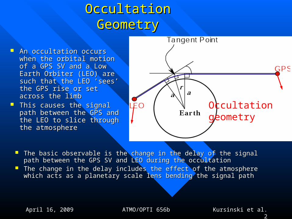
An occultation occurs when An occultation occurs when the orbital motion of a GPS SV the orbital motion of a GPS SV and a Low Earth Orbiter and a Low Earth Orbiter (LEO) are such that the LEO (LEO) are such that the LEO ‘sees’ the GPS rise or set ‘sees’ the GPS rise or set across the limbacross the limb
This causes the signal path This causes the signal path between the GPS and the LEO between the GPS and the LEO to slice through the atmosphereto slice through the atmosphere
Occultation geometry
The basic observable is the change in the delay of the signal path The basic observable is the change in the delay of the signal path between the GPS SV and LEO during the occultationbetween the GPS SV and LEO during the occultation
The change in the delay includes the effect of the atmosphere which acts The change in the delay includes the effect of the atmosphere which acts as a planetary scale lens bending the signal pathas a planetary scale lens bending the signal path
April 16, 2009 ATMO/OPTI 656b Kursinski et al. 3
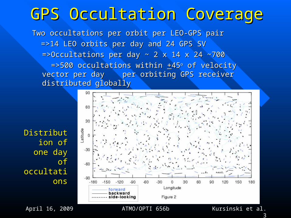
GPS Occultation CoverageGPS Occultation CoverageTwo occultations per orbit per LEO-GPS pairTwo occultations per orbit per LEO-GPS pair
=>14 LEO orbits per day and 24 GPS SV=>14 LEO orbits per day and 24 GPS SV
=>Occultations per day ~ 2 x 14 x 24 ~700=>Occultations per day ~ 2 x 14 x 24 ~700
=>500 occultations within =>500 occultations within ++4545oo of velocity vector per day of velocity vector per day per orbiting GPS receiver distributedper orbiting GPS receiver distributed globallyglobally
Distribution Distribution of one day of of one day of occultationsoccultations
April 16, 2009 ATMO/OPTI 656b Kursinski et al. 4
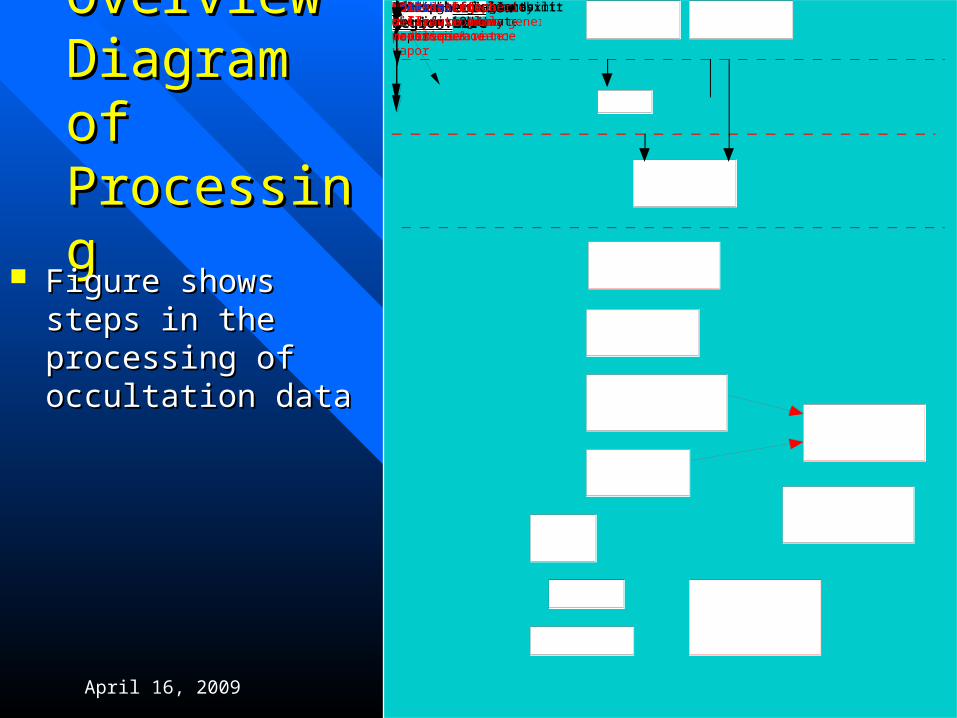
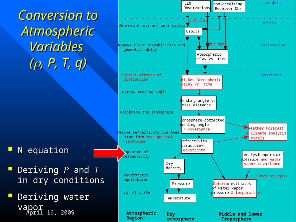
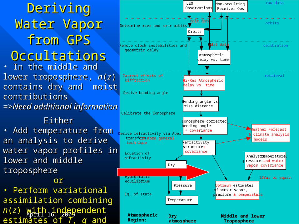
Overview Overview Diagram of Diagram of ProcessingProcessing
Figure shows steps in Figure shows steps in the processing of the processing of occultation dataoccultation data
Remove clock instabilities and geometric delayRefractivity structure + covariance
DrydensityPressureTemperatureOptimum estimates of temperature, pressure & water vapor
HydrostaticequilibriumEq. of stateEquation of refractivityAnalysis temperature, pressure and water vapor + covariance
Middle and lower TroposphereDry atmosphereAtmospheric Region:LEO ObservationsNon-occulting Receiver ObsOrbitsBending angle vs.miss distanceIonosphere corrected bending angle + covariance
Calibrate the Ionosphere Atmospheric delay vs. timeDerive bending angleDetermine rcvr and xmtr orbitsDerive refractivity via Abeltransform or more general technique
Hi-Res Atmospheric delay vs. timeCorrect effects ofDiffraction1DVar or equiv.Weather Forecast & Climate analysis models
raw data orbits calibration retrievaledit dataedit data
April 16, 2009 ATMO/OPTI 656b Kursinski et al. 5
Talk Outline:Talk Outline: Overview of main steps in processing RO signals.Overview of main steps in processing RO signals.
1.1. Occultation GeometryOccultation Geometry
2.2. Abel transform pairAbel transform pair
3.3. Calculation of the bending angles from Doppler.Calculation of the bending angles from Doppler.
4.4. Conversion to atmospheric variables (Conversion to atmospheric variables (, P, T, q), P, T, q)
5.5. Vertical and horizontal resolution of ROVertical and horizontal resolution of RO
6.6. Outline of the main difficulties of RO soundings Outline of the main difficulties of RO soundings (residual ionospheric noise, upper boundary (residual ionospheric noise, upper boundary conditions, multipath, super-refraction)conditions, multipath, super-refraction)
April 16, 2009 ATMO/OPTI 656b Kursinski et al. 6
Abel InversionAbel InversionRemove clock instabilities and geometric delay
Refractivity structure + covariance
Dry density
Pressure
Temperature
Optimum estimates of water vapor, pressure & temperature
Hydrostatic equilibrium
Eq. of state
Equation of refractivity Analysis temperature,
pressure and water vapor + covariance
Middle and lower Troposphere
Dry atmosphere
Atmospheric Region:
LEO Observations
Non-occulting Receiver Obs
Orbits
Bending angle vs. miss distance
Ionosphere corrected bending angle + covariance
Calibrate the Ionosphere
Atmospheric delay vs. time
Derive bending angle
Determine rcvr and xmtr orbits
Derive refractivity via Abel transform or more general technique
Hi-Res Atmospheric delay vs. time
Correct effects of Diffraction
1DVar or equiv.
Weather Forecast & Climate analysis models
raw data
orbits
calibration
retrieval
edit data
edit data
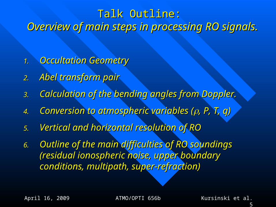
Forward problemForward problem
See also Calc of variations See also Calc of variations (stationary phase) in (stationary phase) in Melbourne et al., 1994Melbourne et al., 1994
Snell’s lawSnell’s law
Forward integral Forward integral
ddnn/d/drr => => ((aa) ) Inverse integral Inverse integral
((aa) => ) => nn((rr))
April 16, 2009 ATMO/OPTI 656b Kursinski et al. 7
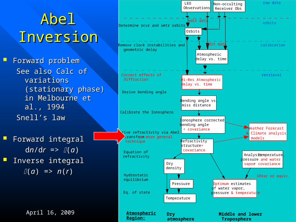
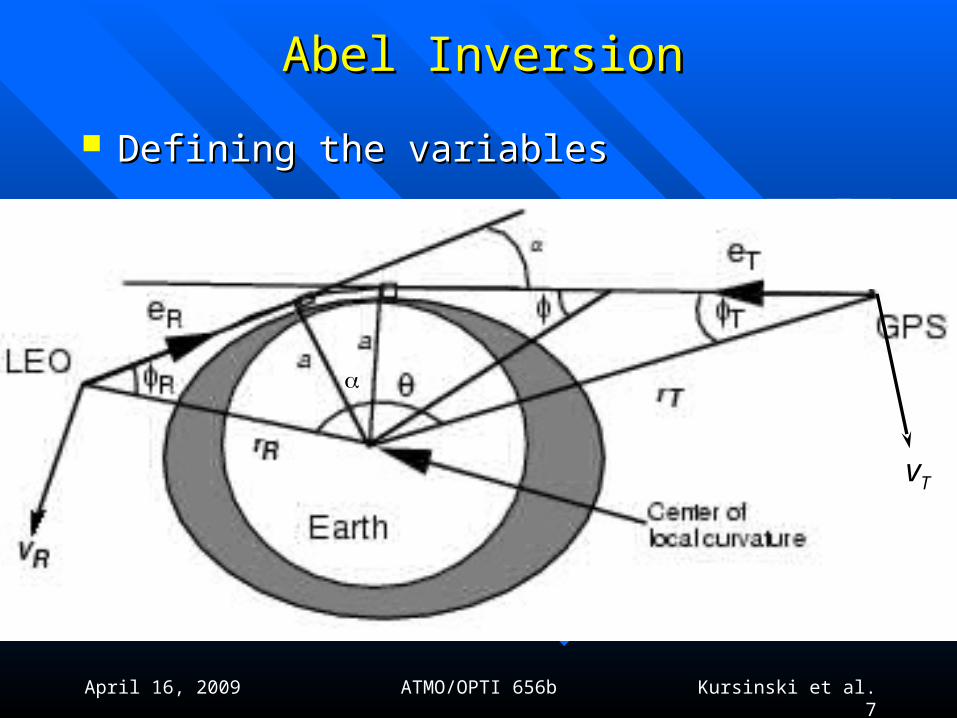
Abel InversionAbel Inversion
Defining the variablesDefining the variables
vT
April 16, 2009 ATMO/OPTI 656b Kursinski et al. 8
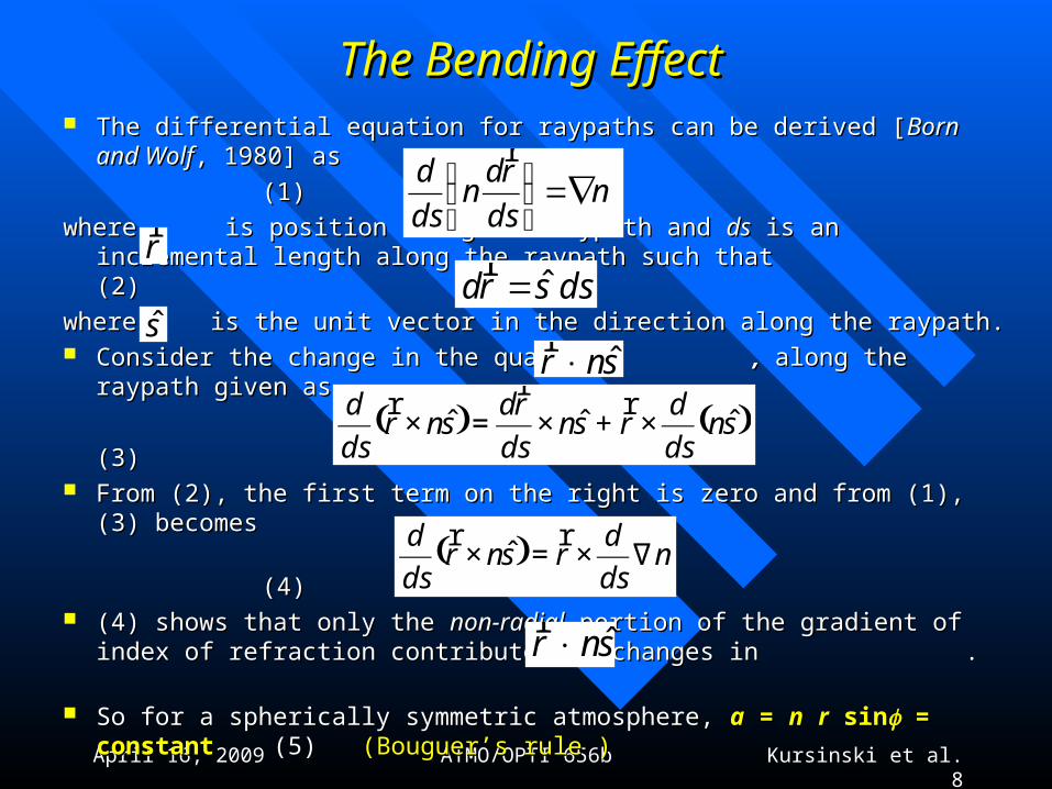
The Bending EffectThe Bending Effect The differential equation for raypaths can be derived [The differential equation for raypaths can be derived [Born and WolfBorn and Wolf, 1980] as, 1980] as
(1)(1)
where is poswhere is posiition along the raypath and tion along the raypath and dsds is an incremental length along the is an incremental length along the raypath such thatraypath such that (2) (2)
where is the unit vector in the direction along the raypath.where is the unit vector in the direction along the raypath. Consider the change in the quantity, Consider the change in the quantity, , , along the raypath given as along the raypath given as
(3)(3) From (2), the first term on the right is zero and from (1), (3) becomesFrom (2), the first term on the right is zero and from (1), (3) becomes
(4)(4) (4) shows that only the (4) shows that only the non-radialnon-radial portion of the gradient of index of refraction portion of the gradient of index of refraction
contributes to changes in . contributes to changes in . So for a spherically symmetric atmosphere, So for a spherically symmetric atmosphere, aa = = nn rr sin sin = constant = constant (5) (5)
(Bouguer’s rule )(Bouguer’s rule )
nds
rdn
ds
d∇=⎟
⎠
⎞⎜⎝
⎛r
dssrd ˆ=rr
r
ssnr ˆ×
r
( ) ( )snds
drsn
ds
rdsnr
ds
dˆˆˆ ×+×=×
rr
r
( ) nds
drsnr
ds
d∇×=×
rrˆ
snr ˆ×r
April 16, 2009 ATMO/OPTI 656b Kursinski et al. 9
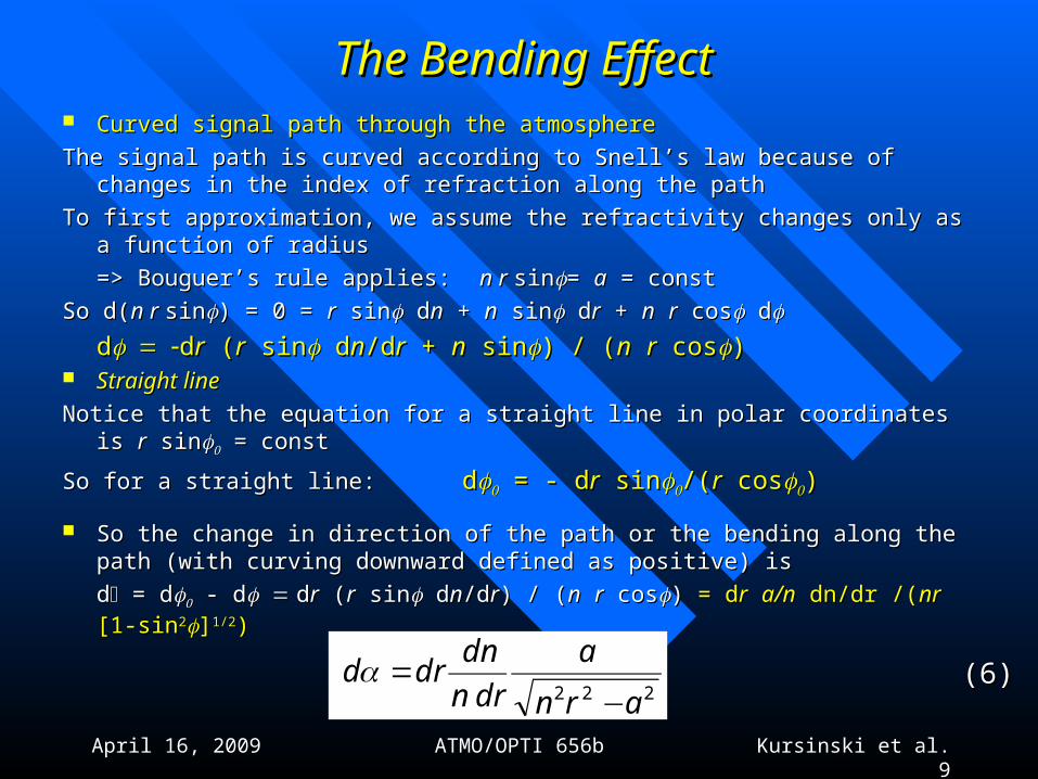
The Bending EffectThe Bending Effect Curved signal path through the atmosphereCurved signal path through the atmosphere
The signal path is curved according to Snell’s law because of changes in the index of The signal path is curved according to Snell’s law because of changes in the index of refraction along the pathrefraction along the path
To first approximation, we assume the refractivity changes only as a function of radius To first approximation, we assume the refractivity changes only as a function of radius
=> Bouguer’s rule applies: => Bouguer’s rule applies: n r n r sinsin= = aa = const = const
So d(So d(n r n r sinsin) = 0 = ) = 0 = rr sin sin d dnn + + nn sin sin d drr + + nn rr cos cos d d
ddddrr ( (rr sin sin d dnn/d/drr + + nn sin sin) / () / (nn rr cos cos)) Straight lineStraight line
Notice that the equation for a straight line in polar coordinates is Notice that the equation for a straight line in polar coordinates is rr sin sin = const = const
So for a straight line: So for a straight line: dd = - d = - drr sin sin/(/(rr cos cos))
So the change in direction of the path or the bending along the path (with curving So the change in direction of the path or the bending along the path (with curving downward defined as positive) is downward defined as positive) is
dd = d = d - d - dddrr ( (rr sin sin d dnn/d/drr) / () / (nn rr cos cos)) = d = drr a/na/n dn/dr /( dn/dr /(nrnr [1-sin [1-sin22]]1/21/2))
222 arn
a
drn
dndrd
−= (6)(6)
April 16, 2009 ATMO/OPTI 656b Kursinski et al. 10
Deducing the Index of Refraction from BendingDeducing the Index of Refraction from Bending
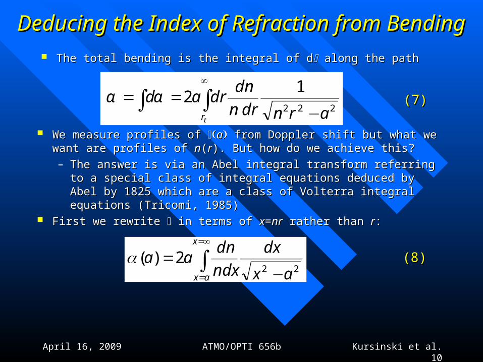
The total bending is the integral of dThe total bending is the integral of d along the path along the path
∫∫∞
−==
tr arndrn
dndrad
222
12αα
We measure profiles of We measure profiles of aa from Doppler shift but what we want are from Doppler shift but what we want are profiles of profiles of nn((rr). But how do we achieve this?). But how do we achieve this?
– The answer is via an Abel integral transform referring to a special The answer is via an Abel integral transform referring to a special class of integral equations deduced by Abel by 1825 which are a class of integral equations deduced by Abel by 1825 which are a class of Volterra integral equations (Tricomi, 1985)class of Volterra integral equations (Tricomi, 1985)
First we rewrite First we rewrite in terms of in terms of xx==nrnr rather than rather than rr::
222)(
ax
dx
ndx
dnaa
x
ax −= ∫
∞=
=
(8)(8)
(7)(7)
April 16, 2009 ATMO/OPTI 656b Kursinski et al. 11
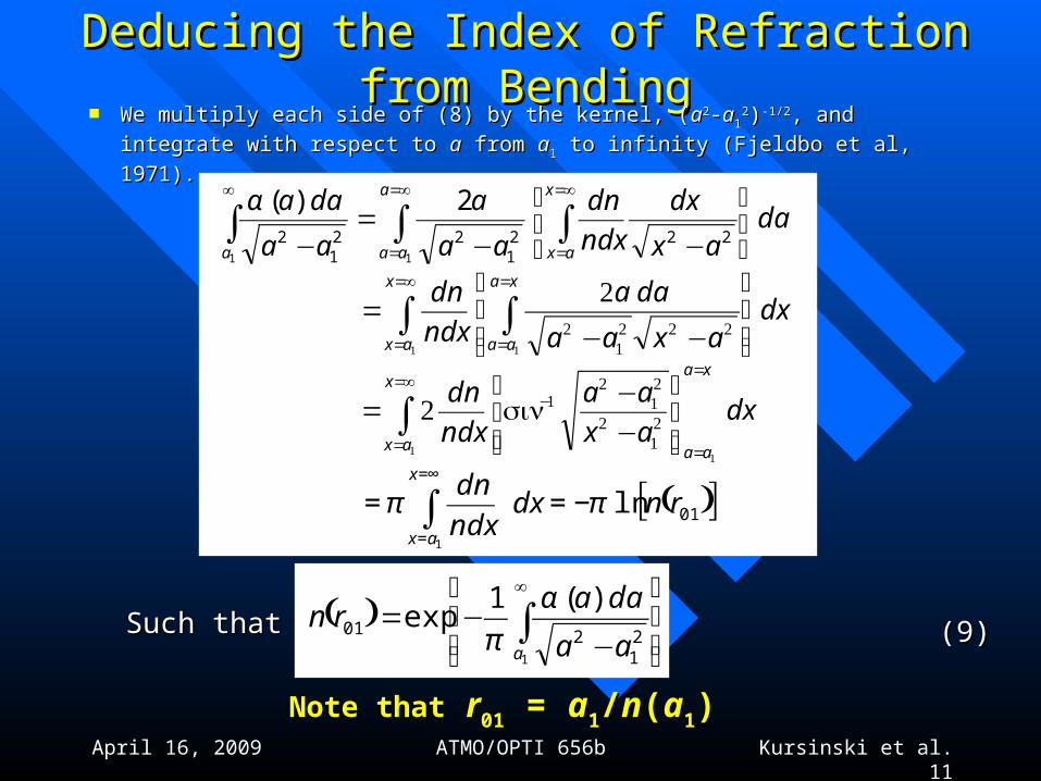
Deducing the Index of Refraction from BendingDeducing the Index of Refraction from Bending We multiply each side of (8) by the kernel, (We multiply each side of (8) by the kernel, (aa22--aa11
22))-1/2-1/2, and integrate with , and integrate with
respect to respect to aa from from aa11 to infinity (Fjeldbo et al, 1971). to infinity (Fjeldbo et al, 1971).
∫ ∫∫∞=
=
∞=
=
∞
⎥⎦
⎤⎢⎣
⎡
−−=
−
a
aa
x
axa
daax
dx
ndx
dn
aa
a
aa
daa
11
2221
221
2
2)(α
dxax
aa
ndx
dnxa
aa
x
ax
=
=
−∞=
= ⎥⎥⎦
⎤
⎢⎢⎣
⎡
−−
= ∫1
1
21
2
21
21sin2
( )[ ]01ln1
rndxndx
dnx
ax
ππ −== ∫∞=
=
dxaxaa
daa
ndx
dn xa
aa
x
ax ⎥⎥⎦
⎤
⎢⎢⎣
⎡
−−= ∫∫
=
=
∞=
= 11
2221
2
2
( )⎥⎥⎦
⎤
⎢⎢⎣
⎡
−−= ∫
∞
1
21
201
)(1exp
a aa
daarn
α
πSuch thatSuch that
Note thatNote that rr0101 = = aa11//nn((aa11))
(9)(9)
April 16, 2009 ATMO/OPTI 656b Kursinski et al. 12
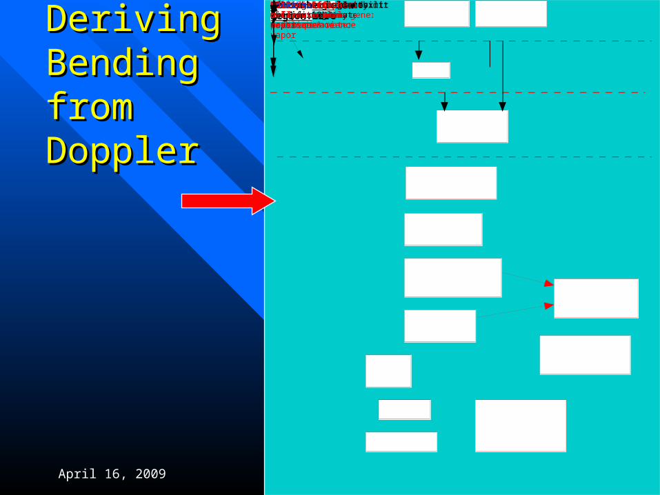
Deriving Deriving Bending from Bending from DopplerDoppler
Remove clock instabilities and geometric delayRefractivity structure + covariance
DrydensityPressureTemperatureOptimum estimates of temperature, pressure & water vapor
HydrostaticequilibriumEq. of stateEquation of refractivityAnalysis temperature, pressure and water vapor + covariance
Middle and lower TroposphereDry atmosphereAtmospheric Region:LEO ObservationsNon-occulting Receiver ObsOrbitsBending angle vs.miss distanceIonosphere corrected bending angle + covariance
Calibrate the Ionosphere Atmospheric delay vs. timeDerive bending angleDetermine rcvr and xmtr orbitsDerive refractivity via Abeltransform or more general technique
Hi-Res Atmospheric delay vs. timeCorrect effects ofDiffraction1DVar or equiv.Weather Forecast & Climate analysis models
raw data orbits calibration retrievaledit dataedit data
April 16, 2009 ATMO/OPTI 656b Kursinski et al. 13
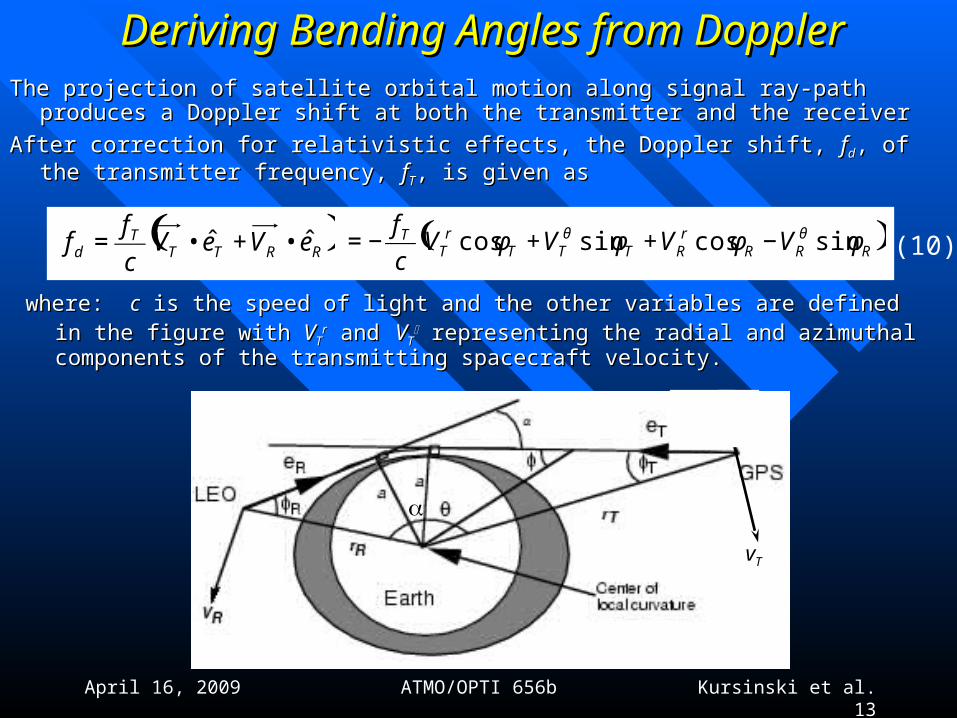
Deriving Bending Angles from DopplerDeriving Bending Angles from DopplerThe projection of satellite orbital motion along signal ray-path produces a Doppler shift at both The projection of satellite orbital motion along signal ray-path produces a Doppler shift at both
the transmitter and the receiverthe transmitter and the receiver
After correction for relativistic effects, the Doppler shift, After correction for relativistic effects, the Doppler shift, ffdd, of the transmitter frequency, , of the transmitter frequency, ffTT, is , is given asgiven as
vT
( )RRTTT
d eVeVc
ff ˆˆ •+•= ( )RRR
rRTTT
rT
T VVVVc
fφφφφ θθ sincossincos −++−=
where: where: cc is the speed of light and the other variables are defined in the figure with is the speed of light and the other variables are defined in the figure with
VVTTrr and and VVTT
representing the radial and azimuthal components of the representing the radial and azimuthal components of the transmitting spacecraft velocity.transmitting spacecraft velocity.
(10)
April 16, 2009 ATMO/OPTI 656b Kursinski et al. 14
Deriving Bending Angles from DopplerDeriving Bending Angles from Doppler
Solve for aSolve for a Under spherical symmetry, Snell's law => Bouguer’s rule (Under spherical symmetry, Snell's law => Bouguer’s rule (Born & WolBorn & Wolf, 1980). f, 1980).
n r n r sin sin = constant = = constant = aa = = n rn rtt
where where rrtt is the radius at the tangent point along the ray path. is the radius at the tangent point along the ray path.
SoSo rrTT sin sin TT = = rrRR sin sin RR = = aa (11)(11)
Given knowledge of the orbital geometry and the center of curvature, we solve Given knowledge of the orbital geometry and the center of curvature, we solve nonlinear equations (10) and (11) iteratively to obtain nonlinear equations (10) and (11) iteratively to obtain TT and and RR andand a a
Solve forSolve forFrom the geometry of the Figure,From the geometry of the Figure, 22 = = TT + + RR + + + +
SoSo = = TT + + RR + + – – (12)(12)
Knowing the geometry which provides Knowing the geometry which provides , the angle between the transmitter and , the angle between the transmitter and the receiver position vectors, we combine the receiver position vectors, we combine TT and and R R in (12) to solve for in (12) to solve for . .
April 16, 2009 ATMO/OPTI 656b Kursinski et al. 15
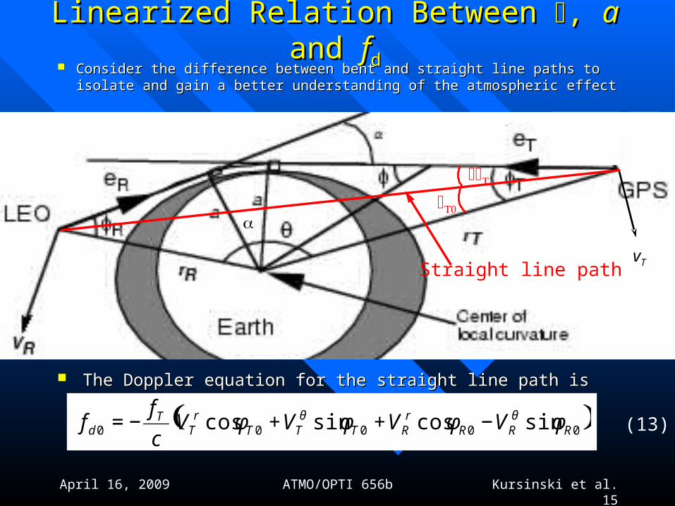
Linearized Relation Between Linearized Relation Between , , aa and and ffdd
Consider the difference between bent and straight line paths to isolate Consider the difference between bent and straight line paths to isolate and gain a better understanding of the atmospheric effectand gain a better understanding of the atmospheric effect
vT
The Doppler equation for the straight line path is The Doppler equation for the straight line path is
( )00000 sincossincos RRRr
RTTTr
TT
d VVVVc
ff φφφφ θθ −++−=
Straight line path
(13)
April 16, 2009 ATMO/OPTI 656b Kursinski et al. 16
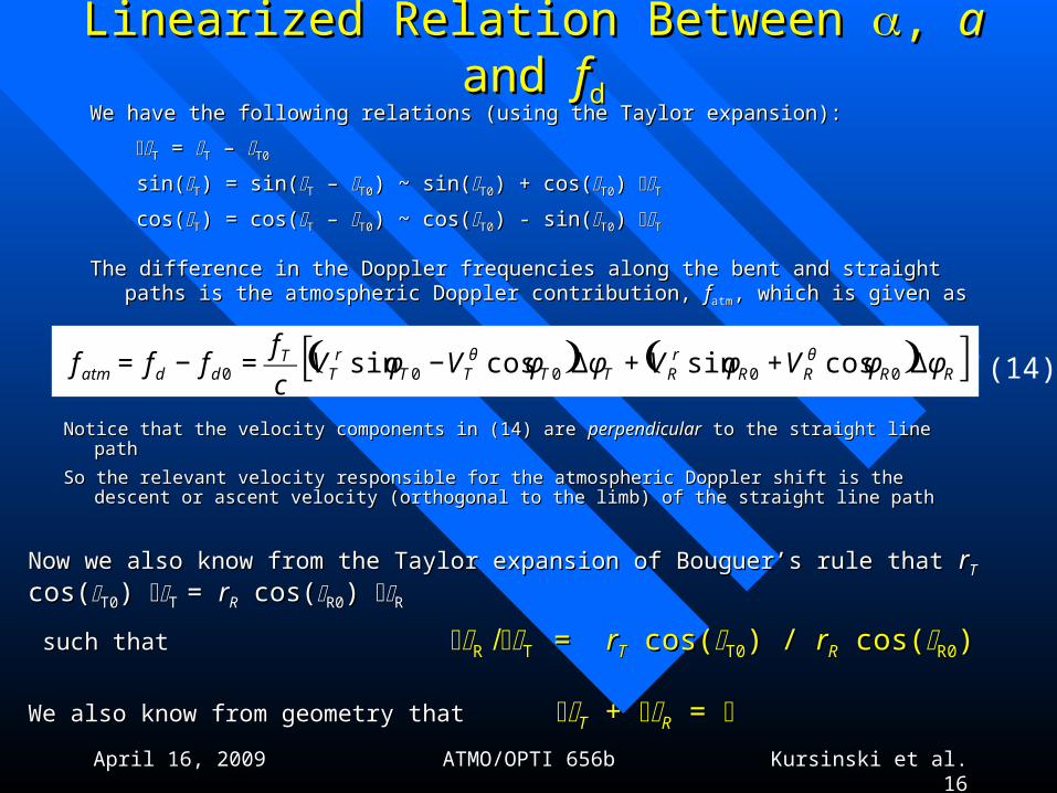
We have the following relations (using the Taylor expansion):We have the following relations (using the Taylor expansion):
TT = = TT – – T0T0
sin(sin(TT) = sin() = sin(TT – – T0T0) ~ sin() ~ sin(T0T0) + cos() + cos(T0T0) ) TT
cos(cos(TT) = cos() = cos(TT – – T0T0) ~ cos() ~ cos(T0T0) - sin() - sin(T0T0) ) TT
The difference in the Doppler frequencies along the bent and straight paths is the atmospheric The difference in the Doppler frequencies along the bent and straight paths is the atmospheric Doppler contribution, Doppler contribution, ffatmatm, which is given as, which is given as
Linearized Relation Between Linearized Relation Between , , aa and and ffdd
( ) ( )[ ]RRRRr
RTTTTr
TT
ddatm VVVVc
ffff φφφφφφ θθ Δ++Δ−=−= 00000 cossincossin
Notice that the velocity components in (14) are Notice that the velocity components in (14) are perpendicularperpendicular to the straight line path to the straight line path
So the relevant velocity responsible for the atmospheric Doppler shift is the descent or ascent So the relevant velocity responsible for the atmospheric Doppler shift is the descent or ascent velocity (orthogonal to the limb) of the straight line pathvelocity (orthogonal to the limb) of the straight line path
(14)
Now we also know from the Taylor expansion of Bouguer’s rule that Now we also know from the Taylor expansion of Bouguer’s rule that rrTT cos( cos(T0T0) ) T T = = rrRR cos( cos(R0R0) ) RR
such thatsuch that R R T T = = rrTT cos( cos(T0T0) / ) / rrRR cos( cos(R0R0))
We also know from geometry that We also know from geometry that TT + + RR = =
April 16, 2009 ATMO/OPTI 656b Kursinski et al. 17
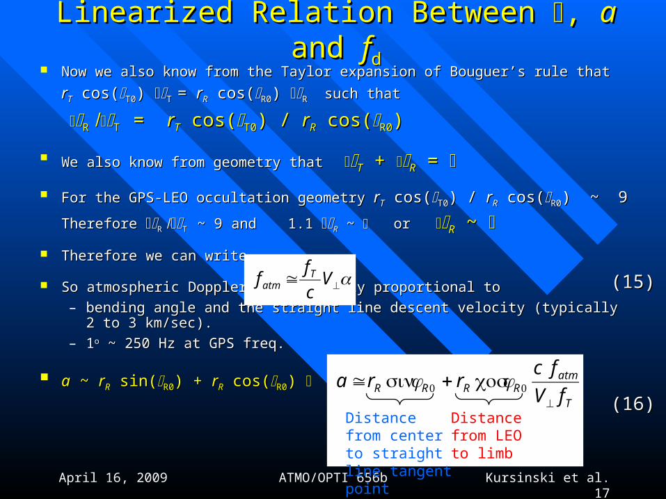
Now we also know from the Taylor expansion of Bouguer’s rule that Now we also know from the Taylor expansion of Bouguer’s rule that
rrTT cos( cos(T0T0) ) T T = = rrRR cos( cos(R0R0) ) RR such that such that
R R T T = = rrTT cos( cos(T0T0) / ) / rrRR cos( cos(R0R0))
We also know from geometry that We also know from geometry that TT + + RR = =
For the GPS-LEO occultation geometry For the GPS-LEO occultation geometry rrTT cos( cos(T0T0) / ) / rrRR cos( cos(R0R0) ~ 9) ~ 9
Therefore Therefore R R T T ~ 9 ~ 9 and and 1.1 1.1 RR ~ ~ or or RR ~ ~
Therefore we can writeTherefore we can write
So atmospheric Doppler is ~ linearly proportional to So atmospheric Doppler is ~ linearly proportional to
– bending angle and the straight line descent velocity (typically 2 to 3 km/sec).bending angle and the straight line descent velocity (typically 2 to 3 km/sec).
– 11oo ~ 250 Hz at GPS freq. ~ 250 Hz at GPS freq.
aa ~ ~ rrRR sin( sin(R0R0) + ) + rrRR cos( cos(R0R0) )
Linearized Relation Between Linearized Relation Between , , aa and and ffdd
⊥≅ Vc
ff T
atm
T
atmRRRR fV
fcrra
⊥
+≅ cossin φφ
Distance from center to straight line tangent point
Distance from LEO to limb
(15)(15)
(16)(16)
April 16, 2009 ATMO/OPTI 656b Kursinski et al. 18
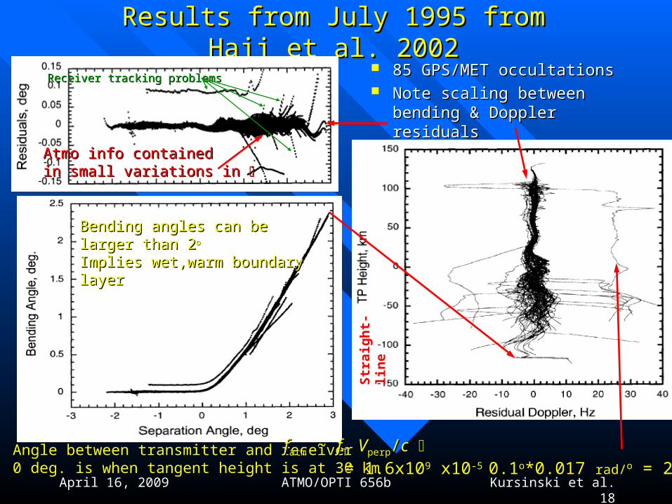
Results from July 1995 from Hajj et al. 2002Results from July 1995 from Hajj et al. 2002 85 GPS/MET occultations85 GPS/MET occultations Note scaling between Note scaling between
bending & Doppler residualsbending & Doppler residuals
Angle between transmitter and receiverAngle between transmitter and receiver0 deg. is when tangent height is at 30 km0 deg. is when tangent height is at 30 km
Receiver tracking problemsReceiver tracking problems
ffatmatm ~ ~ ffTT VVperpperp//cc = 1.6x10= 1.6x1099 x10 x10-5 -5 0.10.1oo*0.017 *0.017 rad/rad/oo = 27 Hz = 27 Hz
Bending angles can be larger than 2Bending angles can be larger than 2oo
Implies wet,warm boundary layerImplies wet,warm boundary layer
Str
aig
ht-
lin
e
Atmo info contained Atmo info contained in small variations in in small variations in
April 16, 2009 ATMO/OPTI 656b Kursinski et al. 19
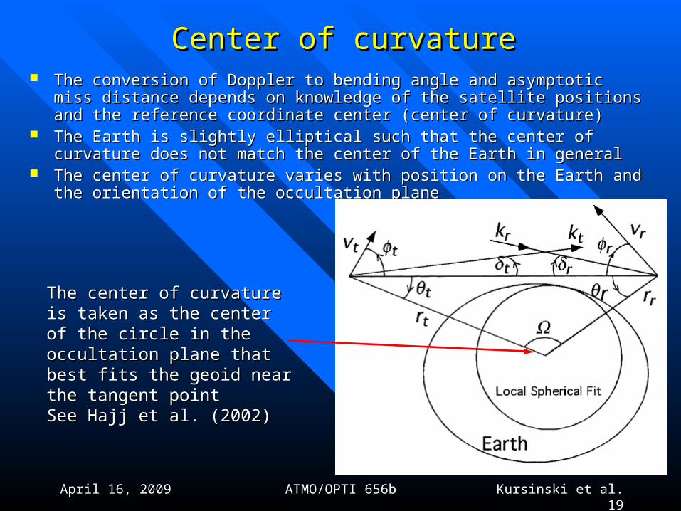
Center of curvatureCenter of curvature The conversion of Doppler to bending angle and asymptotic miss distance depends on The conversion of Doppler to bending angle and asymptotic miss distance depends on
knowledge of the satellite positions and the reference coordinate center (center of knowledge of the satellite positions and the reference coordinate center (center of curvature)curvature)
The Earth is slightly elliptical such that the center of curvature does not match the The Earth is slightly elliptical such that the center of curvature does not match the center of the Earth in generalcenter of the Earth in general
The center of curvature varies with position on the Earth and the orientation of the The center of curvature varies with position on the Earth and the orientation of the occultation planeoccultation plane
The center of curvature is taken as The center of curvature is taken as the center of the circle in the the center of the circle in the occultation plane that best fits the occultation plane that best fits the geoid near the tangent point geoid near the tangent point See Hajj et al. (2002)See Hajj et al. (2002)
April 16, 2009 ATMO/OPTI 656b Kursinski et al. 20
Conversion to Conversion to Atmospheric Atmospheric
Variables Variables ((, P, T, q), P, T, q)
Remove clock instabilities and geometric delay
Refractivity structure + covariance
Dry density
Pressure
Temperature
Optimum estimates of water vapor, pressure & temperature
Hydrostatic equilibrium
Eq. of state
Equation of refractivity Analysis temperature,
pressure and water vapor + covariance
Middle and lower Troposphere
Dry atmosphere
Atmospheric Region:
LEO Observations
Non-occulting Receiver Obs
Orbits
Bending angle vs. miss distance
Ionosphere corrected bending angle + covariance
Calibrate the Ionosphere
Atmospheric delay vs. time
Derive bending angle
Determine rcvr and xmtr orbits
Derive refractivity via Abel transform or more general technique
Hi-Res Atmospheric delay vs. time
Correct effects of Diffraction
1DVar or equiv.
Weather Forecast & Climate analysis models
raw data
orbits
calibration
retrieval
edit data
edit data
N equationN equation
Deriving Deriving PP and and TT in in dry conditionsdry conditions
Deriving water vaporDeriving water vapor
April 16, 2009 ATMO/OPTI 656b Kursinski et al. 21
Conversion to Atmospheric Variables (Conversion to Atmospheric Variables (, P, T, q), P, T, q)
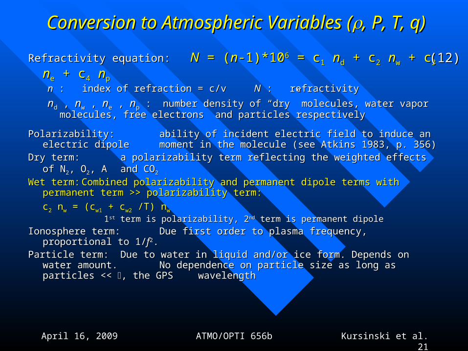
Refractivity equation: Refractivity equation: NN = ( = (nn-1)*10-1)*1066 = c = c11 nndd + c + c22 nnww + c + c3 3 nnee + c + c44 nnpp
nn : index of refraction = c/v : index of refraction = c/v NN : refractivity : refractivity
nndd , , nnww , , nnee , , nnpp : number density of “dry” molecules, water vapor molecules, free : number density of “dry” molecules, water vapor molecules, free electrons electrons and particles respectivelyand particles respectively
Polarizability: Polarizability: ability of incident electric field to induce an electric dipole ability of incident electric field to induce an electric dipole moment in the molecule (see Atkins 1983, p. 356)moment in the molecule (see Atkins 1983, p. 356)
Dry term: Dry term: a polarizability term reflecting the weighted effects of Na polarizability term reflecting the weighted effects of N 22, O, O22, A , A and COand CO22
Wet term:Wet term: Combined polarizability and permanent dipole terms with Combined polarizability and permanent dipole terms with permanent term >> polarizability term:permanent term >> polarizability term:
cc22 n nww = (c = (cw1w1 + c + cw2w2 /T) n /T) nww
11stst term is polarizability, 2 term is polarizability, 2ndnd term is permanent dipole term is permanent dipole
Ionosphere term:Ionosphere term: Due first order to plasma frequency, proportional to 1/Due first order to plasma frequency, proportional to 1/ ff22..Particle term:Particle term: Due to water in liquid and/or ice form. Depends on water amount. Due to water in liquid and/or ice form. Depends on water amount.
No dependence on particle size as long as particles << No dependence on particle size as long as particles << , the GPS , the GPS wavelengthwavelength
(12)(12)
April 16, 2009 ATMO/OPTI 656b Kursinski et al. 22
Conversion to atmospheric variables (Conversion to atmospheric variables (, P, T, q), P, T, q)
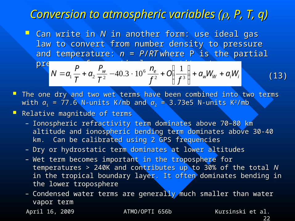
Can write in Can write in NN in another form: use ideal gas law to convert from in another form: use ideal gas law to convert from number density to pressure and temperature: number density to pressure and temperature: nn = = PP//RT RT where P is the where P is the partial pressure of a particular constituentpartial pressure of a particular constituent
The one dry and two wet terms have been combined into two terms with The one dry and two wet terms have been combined into two terms with aa11 = =
77.6 N-units K/mb and 77.6 N-units K/mb and aa22 = 3.73e5 N-units K = 3.73e5 N-units K22/mb/mb
Relative magnitude of termsRelative magnitude of terms
– Ionospheric refractivity term dominates above 70–80 km altitude and Ionospheric refractivity term dominates above 70–80 km altitude and ionospheric bending term dominates above 30-40 km. Can be calibrated ionospheric bending term dominates above 30-40 km. Can be calibrated using 2 GPS frequenciesusing 2 GPS frequencies
– Dry or hydrostatic term dominates at lower altitudesDry or hydrostatic term dominates at lower altitudes
– Wet term becomes important in the troposphere for temperatures > 240K Wet term becomes important in the troposphere for temperatures > 240K and contributes up to 30% of the total and contributes up to 30% of the total NN in the tropical boundary layer. It in the tropical boundary layer. It often dominates bending in the lower troposphereoften dominates bending in the lower troposphere
– Condensed water terms are generally much smaller than water vapor termCondensed water terms are generally much smaller than water vapor term
iiWwew WaWa
fO
f
n
T
Pa
T
PaN ++⎟⎟
⎠
⎞⎜⎜⎝
⎛+×−+= 32
6221
113.4 (13)(13)
April 16, 2009 ATMO/OPTI 656b Kursinski et al. 23
Dry and Wet Contributions to RefractivityDry and Wet Contributions to Refractivity
Example of refractivity from Hilo radiosondeExample of refractivity from Hilo radiosonde• Water contributes up to one third of the total refractivityWater contributes up to one third of the total refractivity
April 16, 2009 ATMO/OPTI 656b Kursinski et al. 24
Deriving Temperature & PressureDeriving Temperature & Pressure
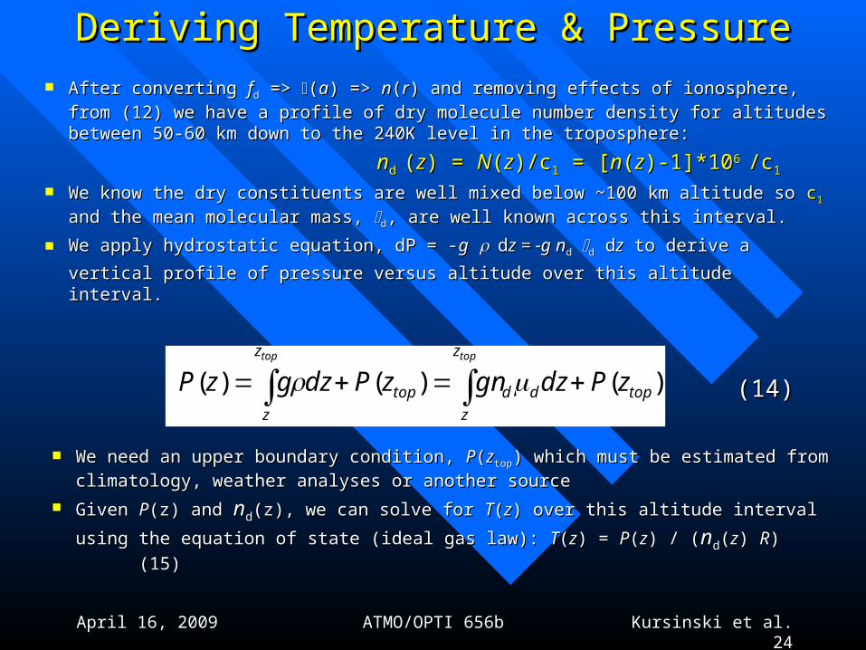
After converting After converting ffdd => => ((aa) => ) => nn((rr) and removing effects of ionosphere, from ) and removing effects of ionosphere, from
(12) we have a profile of dry molecule number density for altitudes between 50-(12) we have a profile of dry molecule number density for altitudes between 50-60 km down to the 240K level in the troposphere:60 km down to the 240K level in the troposphere:
nnd d ((zz) = ) = NN((zz)/c)/c11 = [ = [nn((zz)-1]*10)-1]*106 6 /c/c11
We know the dry constituents are well mixed below ~100 km altitude so We know the dry constituents are well mixed below ~100 km altitude so cc11 and and
the mean molecular mass, the mean molecular mass, dd, are well known across this interval., are well known across this interval.
We apply hydrostatic equation, dP = -We apply hydrostatic equation, dP = -gg ddz = -g nz = -g ndd dd d dzz to derive a vertical to derive a vertical
profile of pressure versus altitude over this altitude interval.profile of pressure versus altitude over this altitude interval.
)()()( top
z
z
ddtop
z
z
zPdzgnzPdzgzPtoptop
+=+= ∫∫ μ
We need an upper boundary condition, We need an upper boundary condition, PP((zztoptop) which must be estimated from ) which must be estimated from
climatology, weather analyses or another sourceclimatology, weather analyses or another source
Given Given PP(z) and (z) and nndd(z), we can solve for (z), we can solve for TT((zz) over this altitude interval using the ) over this altitude interval using the
equation of state (ideal gas law): equation of state (ideal gas law): TT((zz) = ) = PP((zz) / () / (nndd((zz) ) RR)) (15)(15)
(14)(14)
April 16, 2009 ATMO/OPTI 656b Kursinski et al. 25
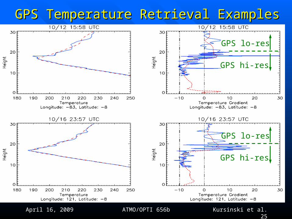
GPS Temperature Retrieval ExamplesGPS Temperature Retrieval Examples
GPS lo-res
GPS hi-res
GPS lo-res
GPS hi-res
26
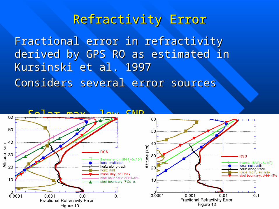
Refractivity ErrorRefractivity Error
Fractional error in refractivity derived by GPS RO as Fractional error in refractivity derived by GPS RO as estimated in Kursinski et al. 1997estimated in Kursinski et al. 1997
Considers several error sourcesConsiders several error sources
Solar max, low SNR Solar min, high SNRSolar max, low SNR Solar min, high SNR
April 16, 2009 ATMO/OPTI 656b Kursinski et al. 27
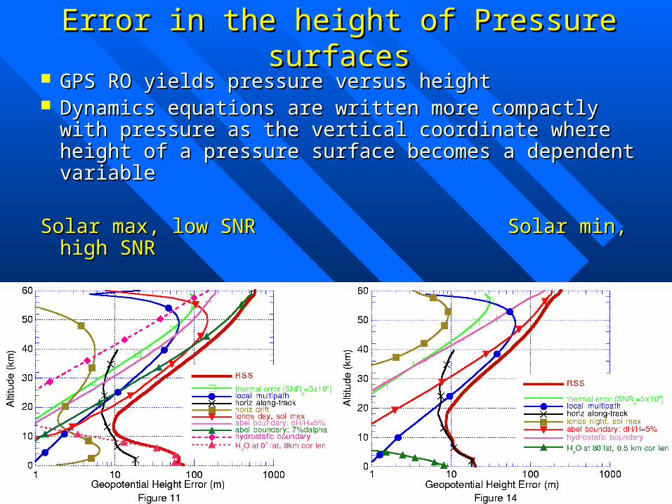
Error in the height of Pressure surfacesError in the height of Pressure surfaces GPS RO yields pressure versus heightGPS RO yields pressure versus height Dynamics equations are written more compactly with Dynamics equations are written more compactly with
pressure as the vertical coordinate where height of a pressure as the vertical coordinate where height of a pressure surface becomes a dependent variablepressure surface becomes a dependent variable
Solar max, low SNR Solar min, high SNRSolar max, low SNR Solar min, high SNR

April 16, 2009 ATMO/OPTI 656b Kursinski et al. 28
GPSRO Temperature AccuracyGPSRO Temperature Accuracy
Temperature is proportional to Pressure/DensityTemperature is proportional to Pressure/Density So So TT/T = /T = PP/P - /P - // Very accurate in upper troposphere/lower troposphere (UTLS)Very accurate in upper troposphere/lower troposphere (UTLS)
Solar max, low SNR Solar min, high SNRSolar max, low SNR Solar min, high SNR
April 16, 2009 ATMO/OPTI 656b Kursinski et al. 29
Deriving Water Deriving Water Vapor from GPS Vapor from GPS
OccultationsOccultations Remove clock instabilities and geometric delay
Refractivity structure + covariance
Dry density
Pressure
Temperature
Optimum estimates of water vapor, pressure & temperature
Hydrostatic equilibrium
Eq. of state
Equation of refractivity Analysis temperature,
pressure and water vapor + covariance
Middle and lower Troposphere
Dry atmosphere
Atmospheric Region:
LEO Observations
Non-occulting Receiver Obs
Orbits
Bending angle vs. miss distance
Ionosphere corrected bending angle + covariance
Calibrate the Ionosphere
Atmospheric delay vs. time
Derive bending angle
Determine rcvr and xmtr orbits
Derive refractivity via Abel transform or more general technique
Hi-Res Atmospheric delay vs. time
Correct effects of Diffraction
1DVar or equiv.
Weather Forecast & Climate analysis models
raw data
orbits
calibration
retrieval
edit data
edit data
• In the middle and lower In the middle and lower troposphere, troposphere, nn((zz) contains dry and ) contains dry and moist contributionsmoist contributions=>Need additional information=>Need additional information
Either Either • Add temperature from an Add temperature from an analysis to derive water vapor analysis to derive water vapor profiles in lower and middle profiles in lower and middle tropospheretroposphere
or or • Perform variational assimilation Perform variational assimilation combining combining nn((zz) with independent ) with independent estimates of estimates of TT, , qq and and PPsurfacesurface and and
covariances of each covariances of each
April 16, 2009 ATMO/OPTI 656b Kursinski et al. 30
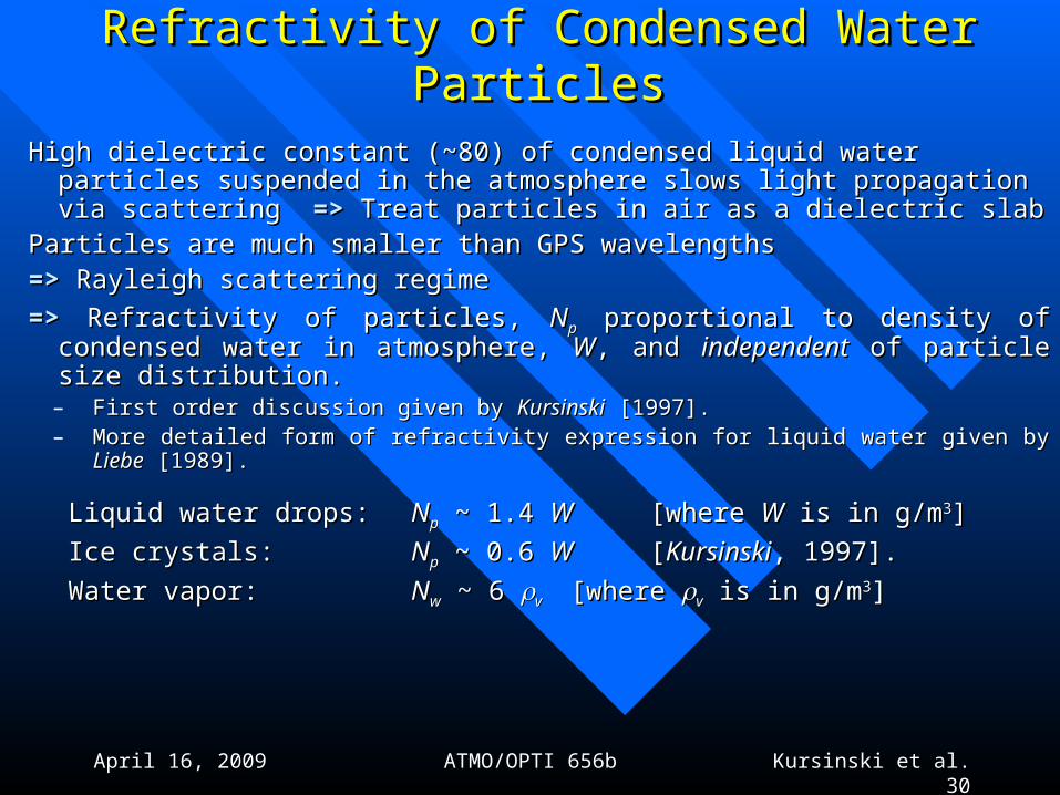
Refractivity of Condensed WaterRefractivity of Condensed Water ParticlesParticles
High dielectric constant (~80) of condensed liquid water particles suspended High dielectric constant (~80) of condensed liquid water particles suspended in the atmosphere slows light propagation via scattering in the atmosphere slows light propagation via scattering =>=> Treat particles Treat particles in air as a dielectric slabin air as a dielectric slab
Particles are much smaller than GPS wavelengths Particles are much smaller than GPS wavelengths =>=> Rayleigh scattering regime Rayleigh scattering regime
=>=> Refractivity of particles, Refractivity of particles, NNpp proportional to density of condensed water in proportional to density of condensed water in atmosphere, atmosphere, WW, and , and independentindependent of particle size distribution. of particle size distribution. – First order discussion given by First order discussion given by KursinskiKursinski [1997]. [1997]. – More detailed form of refractivity expression for liquid water given by More detailed form of refractivity expression for liquid water given by LiebeLiebe [1989]. [1989].
Liquid water drops:Liquid water drops: NNpp ~ 1.4 ~ 1.4 WW [where [where WW is in g/m is in g/m33] ]
Ice crystals:Ice crystals: NNpp ~ 0.6 ~ 0.6 WW [[KursinskiKursinski, 1997]. , 1997].
Water vapor:Water vapor: NNww ~ 6 ~ 6 vv [where [where vv is in g/m is in g/m33]]
April 16, 2009 ATMO/OPTI 656b Kursinski et al. 31
=>=> Same amount of water in vapor phase creates Same amount of water in vapor phase creates ~ 4.4 * refractivity of same amount of liquid water ~ 4.4 * refractivity of same amount of liquid water ~ 10 * refractivity of same amount of water ice~ 10 * refractivity of same amount of water ice
Liquid water content of clouds is generally less than 10% of water Liquid water content of clouds is generally less than 10% of water vapor content (particularly for horizontally extended clouds)vapor content (particularly for horizontally extended clouds)
=>=> Liquid water refractivity generally less than 2.2% of water vapor Liquid water refractivity generally less than 2.2% of water vapor refractivityrefractivity
=>=> Ice clouds generally contribute small fraction of water vapor Ice clouds generally contribute small fraction of water vapor refractivity at altitudes where water vapor contribution is already smallrefractivity at altitudes where water vapor contribution is already small
Clouds will Clouds will veryvery slightly increase apparent water vapor content slightly increase apparent water vapor content
Refractivity of Condensed Water ParticlesRefractivity of Condensed Water Particles
April 16, 2009 ATMO/OPTI 656b Kursinski et al. 32
Deriving Humidity from GPS RODeriving Humidity from GPS RO Two basic approachesTwo basic approaches
– Direct method: use Direct method: use NN & & TT profiles and hydrostatic B.C. profiles and hydrostatic B.C.– Variational method: use Variational method: use NN, , TT & & qq profiles and hydrostatic B.C. profiles and hydrostatic B.C.
with error covariances to update estimates of with error covariances to update estimates of TT, , qq and and PP.. Direct MethodDirect Method
– Theoretically less accurate than variational approachTheoretically less accurate than variational approach– Simple error modelSimple error model– (largely) insensitive to NWP model humidity errors(largely) insensitive to NWP model humidity errors
Variational MethodVariational Method– Theoretically more accurate than simple method because of Theoretically more accurate than simple method because of
inclusion of apriori moisture informationinclusion of apriori moisture information– Sensitive to unknown model humidity errors and biasesSensitive to unknown model humidity errors and biases
Since we are evaluating a model we want water vapor estimates Since we are evaluating a model we want water vapor estimates as independent as possible from modelsas independent as possible from models
=> We use the Direct Method=> We use the Direct Method
April 16, 2009 ATMO/OPTI 656b Kursinski et al. 33
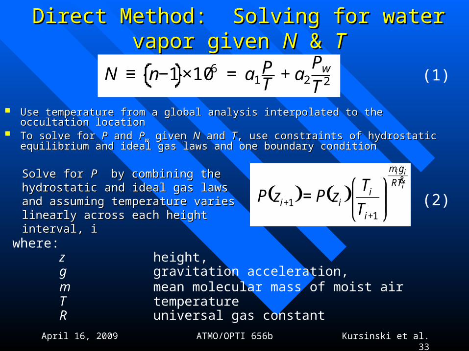
Direct Method: Solving for water vapor Direct Method: Solving for water vapor given given NN & & TT
Use temperature from a global analysis interpolated to the occultation Use temperature from a global analysis interpolated to the occultation locationlocation
To solve for To solve for PP and and PPww given given NN and and TT, use constraints of hydrostatic , use constraints of hydrostatic equilibrium and ideal gas laws and one boundary conditionequilibrium and ideal gas laws and one boundary condition
where:z height,g gravitation acceleration,m mean molecular mass of moist airT temperatureR universal gas constant
(2)
Solve for Solve for PP by combining the by combining the hydrostatic and ideal gas laws and hydrostatic and ideal gas laws and assuming temperature varies assuming temperature varies linearly across each height interval, linearly across each height interval, ii
( ) ( ) i
ii
TR
gm
i
iii T
TzPzP
&
⎟⎟⎠
⎞⎜⎜⎝
⎛=
++
11
N ≡ n−1 ×106 = a1
PT
+ a2Pw
T2 (1)
April 16, 2009 ATMO/OPTI 656b Kursinski et al. 34
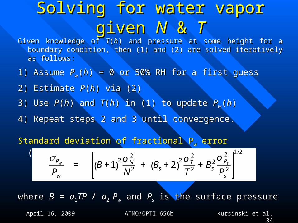
Solving for water vapor given Solving for water vapor given NN & & TTGiven knowledge of Given knowledge of TT((hh) and pressure at some height for a boundary ) and pressure at some height for a boundary
condition, then (1) and (2) are solved iteratively as follows:condition, then (1) and (2) are solved iteratively as follows:
1) Assume 1) Assume PPww((hh) = 0 or 50% RH for a first guess) = 0 or 50% RH for a first guess
2) Estimate 2) Estimate PP((hh) via (2)) via (2)
3) Use 3) Use PP((hh) and ) and TT((hh) in (1) to update ) in (1) to update PPww((hh))
4) Repeat steps 2 and 3 until convergence.4) Repeat steps 2 and 3 until convergence.
Standard deviation of fractional PStandard deviation of fractional Pww error error (Kursinski et al., 1995):(Kursinski et al., 1995):
where where BB = = aa11TP TP / / aa2 2 PPww and and PPss is the surface pressure is the surface pressure
€
σ Pw
Pw
= B +1( )2 σ N
2
N 2+ Bs + 2( )
2 σ T2
T 2+ Bs
2 σ Ps
2
Ps2
⎡
⎣ ⎢
⎤
⎦ ⎥
1/ 2
April 16, 2009 ATMO/OPTI 656b Kursinski et al. 35
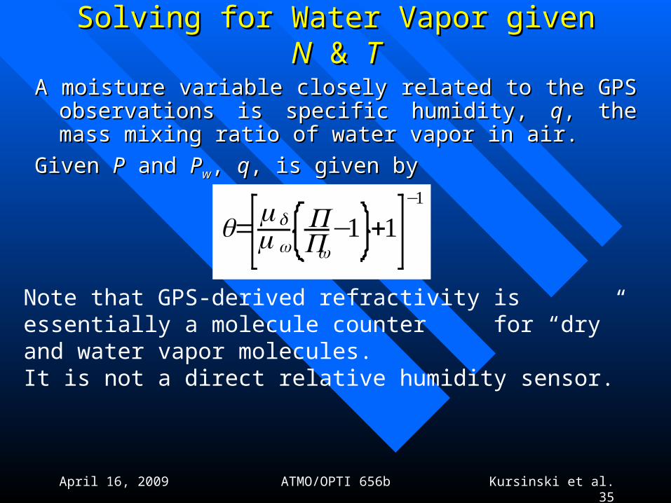
A moisture variable closely related to the GPS observations is A moisture variable closely related to the GPS observations is specific humidity, specific humidity, qq, the mass mixing ratio of water vapor in , the mass mixing ratio of water vapor in air. air.
Given Given PP and and PPww, , qq, is given by, is given by
q=md
mwPPw
−1 +1−1
Solving for Water Vapor given Solving for Water Vapor given NN & & TT
Note that GPS-derived refractivity is essentially a molecule counter for “dry” and water vapor molecules.
It is not a direct relative humidity sensor.
April 16, 2009 ATMO/OPTI 656b Kursinski et al. 37
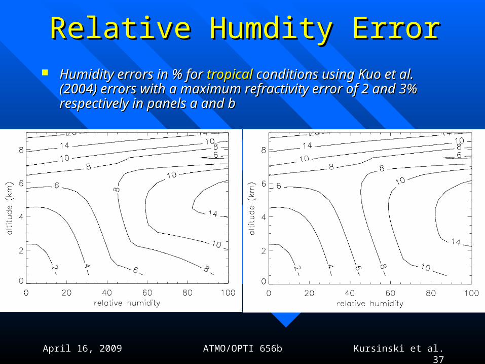
Relative Humdity ErrorRelative Humdity Error Humidity errors in % for Humidity errors in % for tropicaltropical conditions using Kuo et al. (2004) conditions using Kuo et al. (2004)
errors with a maximum refractivity error of 2 and 3% respectively in errors with a maximum refractivity error of 2 and 3% respectively in panels a and bpanels a and b
April 16, 2009 ATMO/OPTI 656b Kursinski et al. 38
Given the GPS observations alone, we have an Given the GPS observations alone, we have an underdeterminedunderdetermined problem in solving for problem in solving for PPww
Previously, we assumed knowledge of temperature to provide the Previously, we assumed knowledge of temperature to provide the missing information & solve this problem.missing information & solve this problem.
However, temperature estimates have errors that we should However, temperature estimates have errors that we should incorporate into our estimateincorporate into our estimate
If we combine If we combine aprioriapriori estimates of temperature estimates of temperature andand water from a water from a forecast or analysis with the GPS refractivity estimates we create forecast or analysis with the GPS refractivity estimates we create an an overdeterminedoverdetermined problem problem
=> => We can use a least squares approach to find the optimal We can use a least squares approach to find the optimal solutions for solutions for TT, , PPww and and P.P.
Variational Estimation of WaterVariational Estimation of Water
April 16, 2009 ATMO/OPTI 656b Kursinski et al. 39
Variational Estimation of WaterVariational Estimation of Water
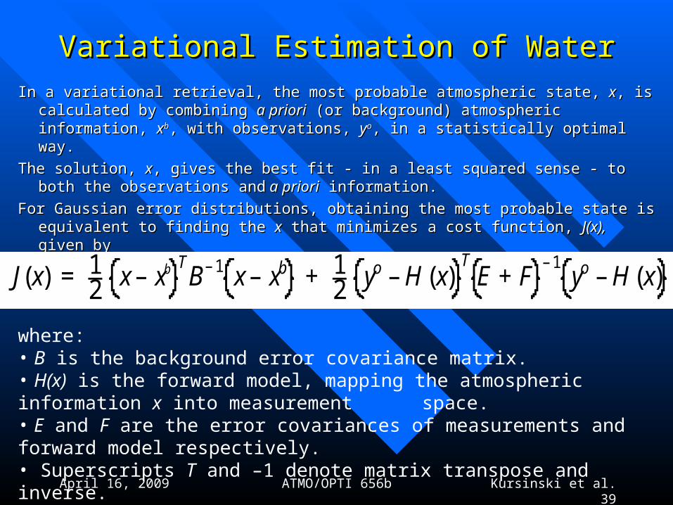
In a variational retrieval, the most probable atmospheric state, In a variational retrieval, the most probable atmospheric state, xx, is calculated by , is calculated by combining combining a prioria priori (or background) atmospheric information, (or background) atmospheric information, xxbb, with , with observations, observations, yyoo, in a statistically optimal way. , in a statistically optimal way.
The solution, The solution, xx, gives the best fit - in a least squared sense - to both the observations , gives the best fit - in a least squared sense - to both the observations andand a priori a priori information. information.
For Gaussian error distributions, obtaining the most probable state is equivalent to For Gaussian error distributions, obtaining the most probable state is equivalent to finding the finding the xx that minimizes a cost function, that minimizes a cost function, J(x),J(x), given by given by
J(x) = 12 x – xb T
B– 1 x – xb + 12 yo – H (x)
TE + F
– 1yo – H (x)
where:• B is the background error covariance matrix.• H(x) is the forward model, mapping the atmospheric information x into measurement space.• E and F are the error covariances of measurements and forward model respectively. • Superscripts T and –1 denote matrix transpose and inverse.
April 16, 2009 ATMO/OPTI 656b Kursinski et al. 40
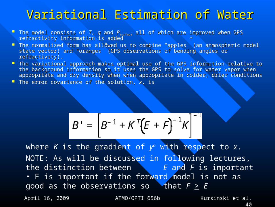
The model consists of The model consists of TT, , qq and and PPsurfacesurface all of which are improved when GPS refractivity all of which are improved when GPS refractivity information is addedinformation is added
The normalized form has allowed us to combine “apples” (an atmospheric model state The normalized form has allowed us to combine “apples” (an atmospheric model state vector) and “oranges” (GPS observations of bending angles or refractivity). vector) and “oranges” (GPS observations of bending angles or refractivity).
The variational approach makes optimal use of the GPS information relative to the The variational approach makes optimal use of the GPS information relative to the background information so it uses the GPS to solve for water vapor when appropriate and background information so it uses the GPS to solve for water vapor when appropriate and dry density when when appropriate in colder, drier conditionsdry density when when appropriate in colder, drier conditions
The error covariance of the solution, The error covariance of the solution, xx, is, is
Variational Estimation of WaterVariational Estimation of Water
B' = B– 1 + K T E + F
– 1K
– 1
where K is the gradient of yo with respect to x.
NOTE: As will be discussed in following lectures, the distinction between E and F is important
• F is important if the forward model is not as good as the observations so that F > E
April 16, 2009 ATMO/OPTI 656b Kursinski et al. 41
Variational Estimation of Water: Variational Estimation of Water: Advantages & DisadvantagesAdvantages & Disadvantages
The solution is theoretically better than the solution The solution is theoretically better than the solution assuming only temperatureassuming only temperature
The solution is limited to the model levels and GPS The solution is limited to the model levels and GPS generally has higher vertical resolution than modelsgenerally has higher vertical resolution than models
The solution is as good as its assumptionsThe solution is as good as its assumptions
– Unbiased aprioriUnbiased apriori
– Correct error covariancesCorrect error covariances Model constraints are significant in defining the apriori Model constraints are significant in defining the apriori
water estimates and may therefore yield unwanted model water estimates and may therefore yield unwanted model biases in the resultsbiases in the results
Temperature approach provides more independent Temperature approach provides more independent estimate of water vaporestimate of water vapor
April 16, 2009 ATMO/OPTI 656b Kursinski et al. 42
Vertical and Horizontal Resolution of ROVertical and Horizontal Resolution of RO
Resolution associated with distributed Resolution associated with distributed bending along the raypathbending along the raypath
Diffraction limited vertical resolutionDiffraction limited vertical resolution Horizontal resolutionHorizontal resolution
April 16, 2009 ATMO/OPTI 656b Kursinski et al. 43
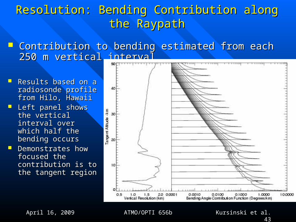
Resolution: Bending Contribution along the RaypathResolution: Bending Contribution along the Raypath
Contribution to bending estimated from each 250 m vertical Contribution to bending estimated from each 250 m vertical intervalinterval
Results based on a Results based on a radiosonde profile from radiosonde profile from Hilo, HawaiiHilo, Hawaii
Left panel shows the Left panel shows the vertical interval over vertical interval over which half the bending which half the bending occursoccurs
Demonstrates how Demonstrates how focused the focused the contribution is to the contribution is to the tangent regiontangent region
April 16, 2009 ATMO/OPTI 656b Kursinski et al. 44
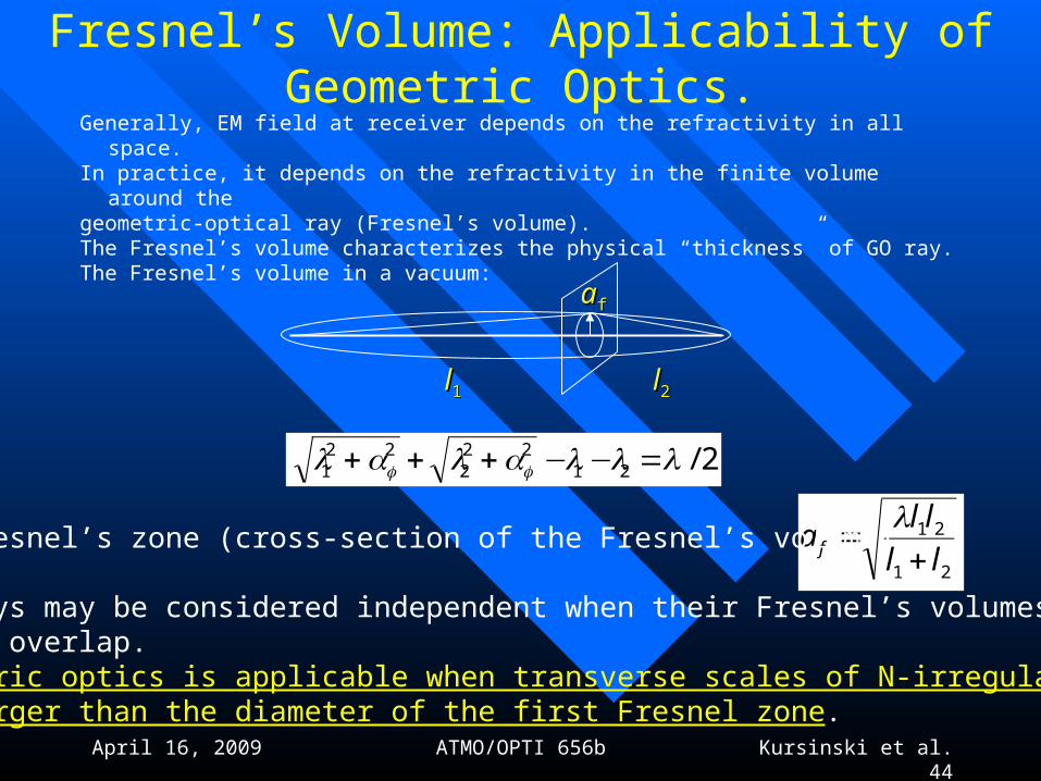
Fresnel’s Volume: Applicability of Geometric Optics.Generally, EM field at receiver depends on the refractivity in all space.In practice, it depends on the refractivity in the finite volume around thegeometric-optical ray (Fresnel’s volume).The Fresnel’s volume characterizes the physical “thickness” of GO ray.The Fresnel’s volume in a vacuum:
aaff
ll22ll11
2/2122
222
1 λ=−−+++ llalal ff
21
21
ll
lla f +
=λ
The Fresnel’s zone (cross-section of the Fresnel’s volume):
Two rays may be considered independent when their Fresnel’s volumesdo not overlap.Geometric optics is applicable when transverse scales of N-irregularitiesare larger than the diameter of the first Fresnel zone.
April 16, 2009 ATMO/OPTI 656b Kursinski et al. 45
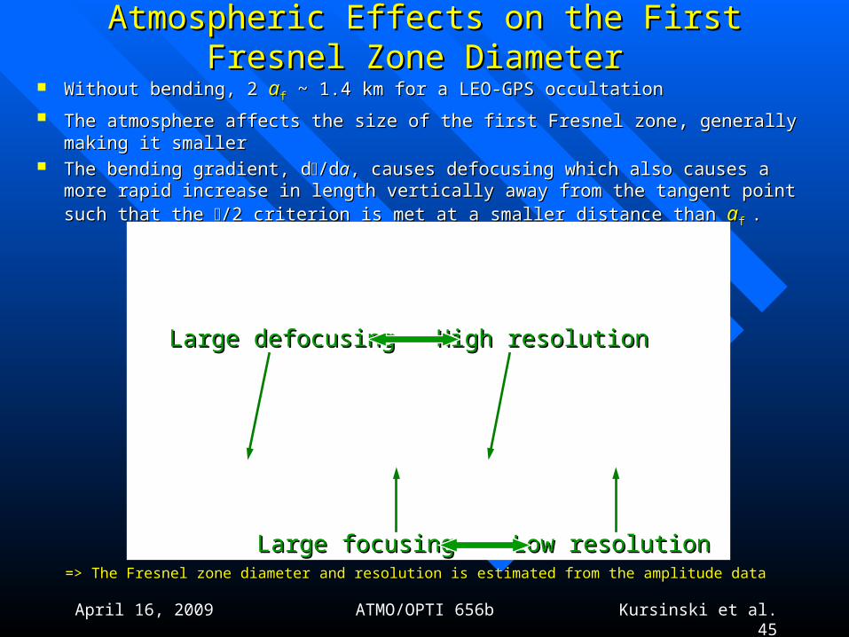
Atmospheric Effects on the First Fresnel Zone Diameter Atmospheric Effects on the First Fresnel Zone Diameter
Without bending, 2 Without bending, 2 aaff ~ 1.4 km for a LEO-GPS occultation ~ 1.4 km for a LEO-GPS occultation
The atmosphere affects the size of the first Fresnel zoneThe atmosphere affects the size of the first Fresnel zone ,, generally making it smaller generally making it smaller The bending gradient, dThe bending gradient, d/d/daa, causes defocusing which also causes a more rapid , causes defocusing which also causes a more rapid
increase in length vertically away from the tangent point such that the increase in length vertically away from the tangent point such that the /2 criterion is /2 criterion is met at a smaller distance than met at a smaller distance than aaff . .
=> The Fresnel zone diameter and resolution is estimated from the amplitude data=> The Fresnel zone diameter and resolution is estimated from the amplitude data
Large defocusingLarge defocusing High resolutionHigh resolution
Large focusingLarge focusing Low resolutionLow resolution
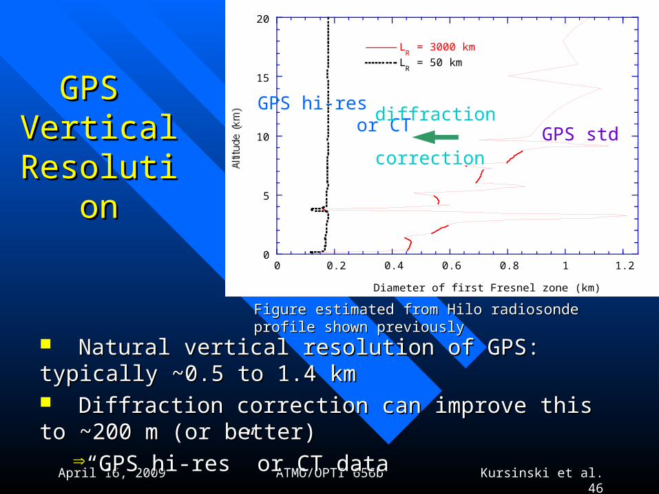
April 16, 2009 ATMO/OPTI 656b Kursinski et al. 46
GPS GPS Vertical Vertical
ResolutionResolution
0 0.2 0.4 0.6 0.8 1 1.20
5
10
15
20
LR = 3000 km
LR = 50 km
Diameter of first Fresnel zone (km)
GPS std
GPS hi-res or CT
Natural vertical resolution of GPS: typically ~0.5 to 1.4 km Natural vertical resolution of GPS: typically ~0.5 to 1.4 km Diffraction correction can improve this to ~200 m (or better)Diffraction correction can improve this to ~200 m (or better)
““GPS hi-res” or CT data GPS hi-res” or CT data
diffraction
correction
Figure estimated from Hilo radiosonde profile shown previouslyFigure estimated from Hilo radiosonde profile shown previously
April 16, 2009 ATMO/OPTI 656b Kursinski et al. 47
Horizontal ResolutionHorizontal Resolution
Different approaches to estimating itDifferent approaches to estimating it
– Gaussian horizontal bending contribution:Gaussian horizontal bending contribution: ++300 km300 km
– Horizontal interval of half the bending occurs: ~300 kmHorizontal interval of half the bending occurs: ~300 km
– Horizontal interval of natural Fresnel zone: Horizontal interval of natural Fresnel zone: ~250 km~250 km
– Horizontal interval of diffraction corrected, Horizontal interval of diffraction corrected,
200 m Fresnel zone: (Probably not realistic) 200 m Fresnel zone: (Probably not realistic) ~100 km ~100 km
Overall approximate estimate is ~ 300 kmOverall approximate estimate is ~ 300 km
April 16, 2009 ATMO/OPTI 656b Kursinski et al. 48
Intro to Difficulties of RO soundingsIntro to Difficulties of RO soundings
Residual ionospheric noiseResidual ionospheric noise Multipath, Multipath, SuperrefractionSuperrefraction Upper boundary conditionsUpper boundary conditions
April 16, 2009 ATMO/OPTI 656b Kursinski et al. 49
Ionospheric Ionospheric CorrectionCorrection
Remove clock instabilities and geometric delayRefractivity structure + covariance
DrydensityPressureTemperatureOptimum estimates of temperature, pressure & water vapor
HydrostaticequilibriumEq. of stateEquation of refractivityAnalysis temperature, pressure and water vapor + covariance
Middle and lower TroposphereDry atmosphereAtmospheric Region:LEO ObservationsNon-occulting Receiver ObsOrbitsBending angle vs.miss distanceIonosphere corrected bending angle + covariance
Calibrate the Ionosphere Atmospheric delay vs. timeDerive bending angleDetermine rcvr and xmtr orbitsDerive refractivity via Abeltransform or more general technique
Hi-Res Atmospheric delay vs. timeCorrect effects ofDiffraction1DVar or equiv.Weather Forecast & Climate analysis models
raw data orbits calibration retrievaledit dataedit data
April 16, 2009 ATMO/OPTI 656b Kursinski et al. 50
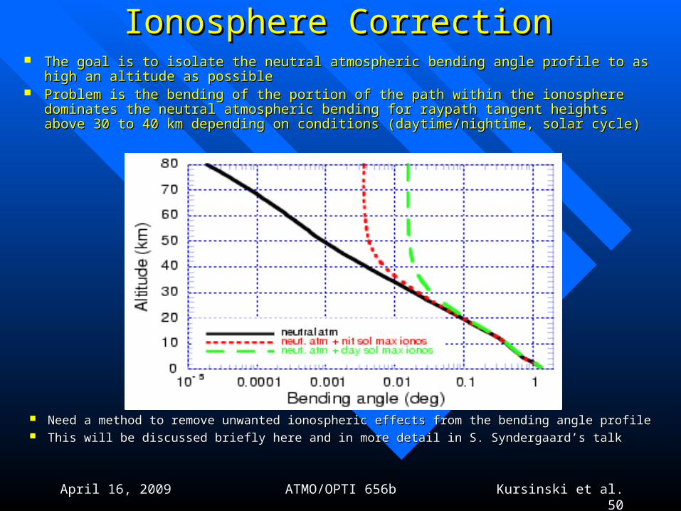
Ionosphere CorrectionIonosphere Correction The goal is to isolate the neutral atmospheric bending angle profile to as high an altitude as possibleThe goal is to isolate the neutral atmospheric bending angle profile to as high an altitude as possible Problem is the bending of the portion of the path within the ionosphere dominates the neutral Problem is the bending of the portion of the path within the ionosphere dominates the neutral
atmospheric bending for raypath tangent heights above 30 to 40 km depending on conditions atmospheric bending for raypath tangent heights above 30 to 40 km depending on conditions (daytime/nightime, solar cycle)(daytime/nightime, solar cycle)
Need a method to remove unwanted ionospheric effects from the bending angle profileNeed a method to remove unwanted ionospheric effects from the bending angle profile This will be discussed briefly here and in more detail in S. Syndergaard’s talkThis will be discussed briefly here and in more detail in S. Syndergaard’s talk
April 16, 2009 ATMO/OPTI 656b Kursinski et al. 51
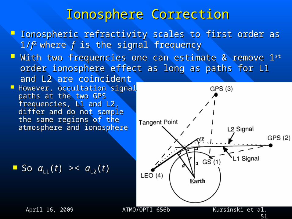
Ionosphere CorrectionIonosphere Correction Ionospheric refractivity scales to first order as 1/Ionospheric refractivity scales to first order as 1/ff2 2 where where ff is the is the
signal frequencysignal frequency With two frequencies one can estimate & remove 1With two frequencies one can estimate & remove 1stst order order
ionosphere effect as long as paths for L1 and L2 are coincidentionosphere effect as long as paths for L1 and L2 are coincident
So So aaL1L1((tt) >< ) >< aaL2L2((tt))
However, occultation signal However, occultation signal paths at the two GPS paths at the two GPS frequencies, L1 and L2, differ frequencies, L1 and L2, differ and do not sample the same and do not sample the same regions of the atmosphere and regions of the atmosphere and ionosphereionosphere
April 16, 2009 ATMO/OPTI 656b Kursinski et al. 52
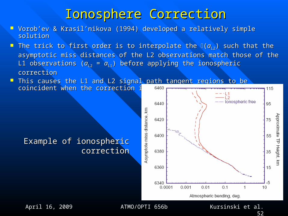
Vorob’ev & Krasil’nikova (1994) developed a relatively simple solution Vorob’ev & Krasil’nikova (1994) developed a relatively simple solution
The trick to first order is to interpolate the The trick to first order is to interpolate the ((aaL2L2) such that the asymptotic ) such that the asymptotic
miss distances of the L2 observations match those of the L1 observations miss distances of the L2 observations match those of the L1 observations ((aaL2L2 = = aaL1L1) before applying the ionospheric correction) before applying the ionospheric correction
This causes the L1 and L2 signal path tangent regions to be coincident This causes the L1 and L2 signal path tangent regions to be coincident when the correction is appliedwhen the correction is applied
Ionosphere CorrectionIonosphere Correction
Example of ionospheric correctionExample of ionospheric correction

53
Refractivity ErrorRefractivity Error
Fractional error in refractivity derived by GPS RO as Fractional error in refractivity derived by GPS RO as estimated in Kursinski et al. 1997estimated in Kursinski et al. 1997
Considers several error sourcesConsiders several error sources
Solar max, low SNR Solar min, high SNRSolar max, low SNR Solar min, high SNR
April 16, 2009 ATMO/OPTI 656b Kursinski et al. 54
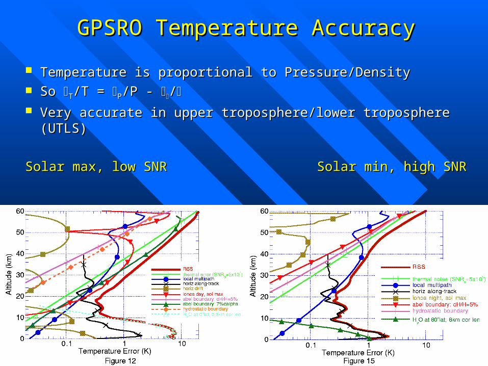
GPSRO Temperature AccuracyGPSRO Temperature Accuracy
Temperature is proportional to Pressure/DensityTemperature is proportional to Pressure/Density So So TT/T = /T = PP/P - /P - // Very accurate in upper troposphere/lower troposphere (UTLS)Very accurate in upper troposphere/lower troposphere (UTLS)
Solar max, low SNR Solar min, high SNRSolar max, low SNR Solar min, high SNR
April 16, 2009 ATMO/OPTI 656b Kursinski et al. 55
Reducing the ionospheric effect of the solar cycleReducing the ionospheric effect of the solar cycle
With the current ionospheric calibration approach, a subtle With the current ionospheric calibration approach, a subtle systematic ionospheric residual effect is left in the bending systematic ionospheric residual effect is left in the bending angle profileangle profile
This effect is large compared to predicted decadal climate This effect is large compared to predicted decadal climate signatures ~0.1K/decadesignatures ~0.1K/decade
The residual ionosphere effect is due to an overcorrection of The residual ionosphere effect is due to an overcorrection of the ionospheric effectthe ionospheric effect
This causes the ionospherically corrected bending angle to This causes the ionospherically corrected bending angle to change sign and become slightly negative.change sign and become slightly negative.
This negative bending can be averaged and subtracted from the This negative bending can be averaged and subtracted from the bending angle profile to largely remove the biasbending angle profile to largely remove the bias
This idea needs further work but appears promisingThis idea needs further work but appears promising
April 16, 2009 ATMO/OPTI 656b Kursinski et al. 56
Upper Boundary ConditionsUpper Boundary Conditions
We have two upper boundary conditions to contend with: We have two upper boundary conditions to contend with: the Abel integral and the hydrostatic integral.the Abel integral and the hydrostatic integral.
For the Abel, we can either extrapolate the bending angle For the Abel, we can either extrapolate the bending angle profile to higher altitudes or combine the data with profile to higher altitudes or combine the data with climatological or weather analysis informationclimatological or weather analysis information
Hydrostatic integral requires knowledge of pressure near the Hydrostatic integral requires knowledge of pressure near the stratopause. Typical approach is to use an estimate of stratopause. Typical approach is to use an estimate of temperature combined with refractivity derived from GPS temperature combined with refractivity derived from GPS to determine pressure.to determine pressure.
Problem with using a climatology is it may introduce a biasProblem with using a climatology is it may introduce a bias Also a basic challenge is to determine, based on the data Also a basic challenge is to determine, based on the data
accuracy, at what altitude to start the abel and hydrostatic accuracy, at what altitude to start the abel and hydrostatic integralsintegrals
April 16, 2009 ATMO/OPTI 656b Kursinski et al. 57
Atmospheric MultipathAtmospheric Multipath
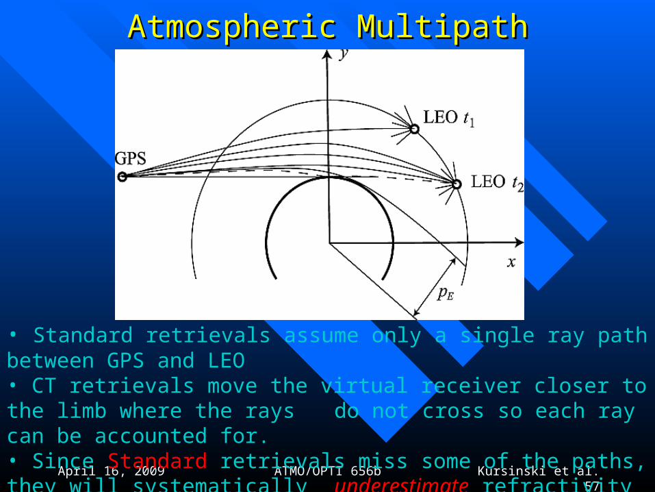
• Standard retrievals assume only a single ray path between GPS and LEO• CT retrievals move the virtual receiver closer to the limb where the rays
do not cross so each ray can be accounted for.• Since Standard retrievals miss some of the paths, they will systematically
underestimate refractivity in regions where multipath occurs.
April 16, 2009 ATMO/OPTI 656b Kursinski et al. 58
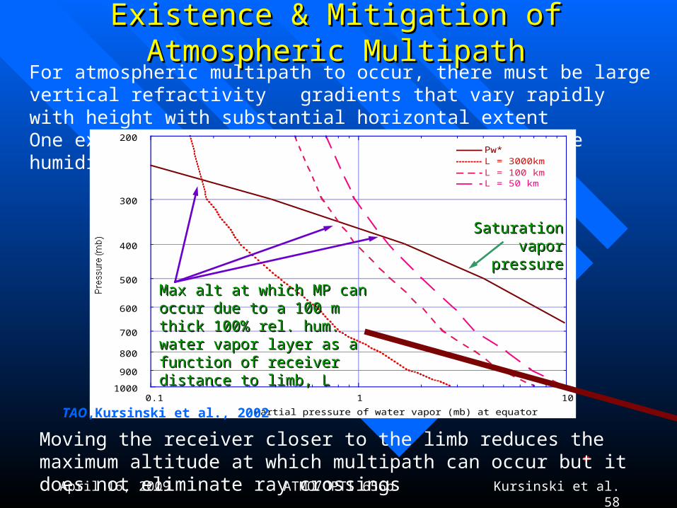
Existence & Mitigation of Atmospheric MultipathExistence & Mitigation of Atmospheric MultipathFor atmospheric multipath to occur, there must be large vertical refractivity gradients that vary rapidly with height with substantial horizontal extent One expects multipath in regions of high absolute humidity
0.1 1 10
200
300
400
500
600
700
800
900
1000
Pw*L = 3000kmL = 100 kmL = 50 km
Partial pressure of water vapor (mb) at equator
Pressure (mb)
Saturation vapor Saturation vapor pressurepressure
Moving the receiver closer to the limb reduces the maximum altitude at which multipath can occur but it does not eliminate ray crossings
TAO,Kursinski et al., 2002
Max alt at which MP can occur due Max alt at which MP can occur due to a 100 m thick 100% rel. hum. to a 100 m thick 100% rel. hum. water vapor layer as a function of water vapor layer as a function of receiver distance to limb, Lreceiver distance to limb, L
April 16, 2009 ATMO/OPTI 656b Kursinski et al. 59
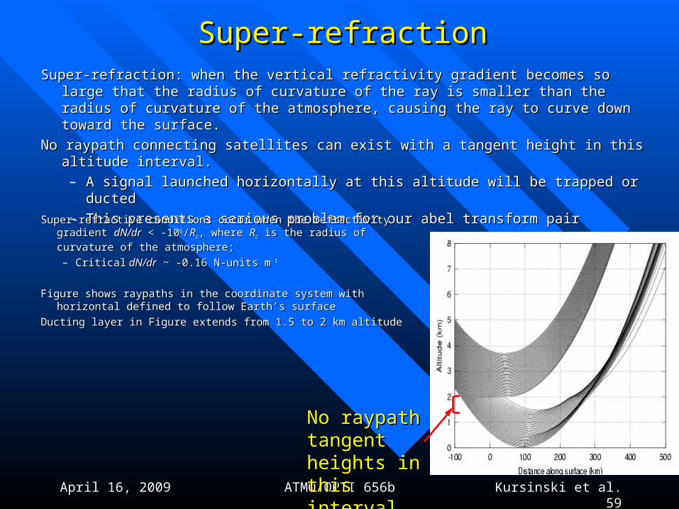
Super-refractionSuper-refractionSuper-refraction: when the vertical refractivity gradient becomes so large that the radius Super-refraction: when the vertical refractivity gradient becomes so large that the radius
of curvature of the ray is smaller than the radius of curvature of the atmosphere, of curvature of the ray is smaller than the radius of curvature of the atmosphere, causing the ray to curve down toward the surface. causing the ray to curve down toward the surface.
No raypath connecting satellites can exist with a tangent height in this altitude interval. No raypath connecting satellites can exist with a tangent height in this altitude interval.
– A signal launched horizontally at this altitude will be trapped or ductedA signal launched horizontally at this altitude will be trapped or ducted
– This presents a serious problem for our abel transform pairThis presents a serious problem for our abel transform pair
Super-refractive conditions occur when the refractivity gradient Super-refractive conditions occur when the refractivity gradient dN/drdN/dr < -10< -1066//RRcc, where , where RRcc is the radius of curvature of the atmosphere; is the radius of curvature of the atmosphere;
– CriticalCritical dN/dr dN/dr ~ -0.16 N-units m ~ -0.16 N-units m-1-1
Figure shows raypaths in the coordinate system with horizontal Figure shows raypaths in the coordinate system with horizontal defined to follow Earth’s surfacedefined to follow Earth’s surface
Ducting layer in Figure extends from 1.5 to 2 km altitudeDucting layer in Figure extends from 1.5 to 2 km altitude
No raypath No raypath tangent heights tangent heights in this intervalin this interval
April 16, 2009 ATMO/OPTI 656b Kursinski et al. 60
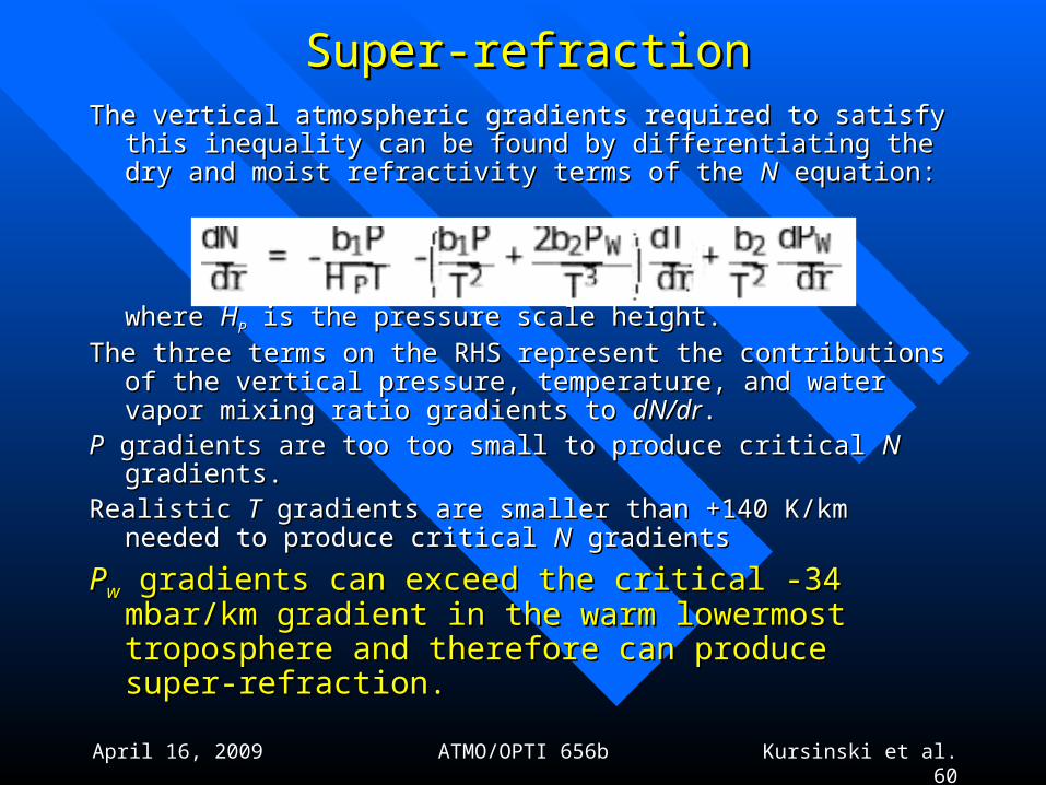
Super-refractionSuper-refractionThe vertical atmospheric gradients required to satisfy this inequality can The vertical atmospheric gradients required to satisfy this inequality can
be found by differentiating the dry and moist refractivity terms of the be found by differentiating the dry and moist refractivity terms of the NN equation: equation:
where where HHPP is the pressure scale height. is the pressure scale height.
The three terms on the RHS represent the contributions of the vertical The three terms on the RHS represent the contributions of the vertical pressure, temperature, and water vapor mixing ratio gradients to pressure, temperature, and water vapor mixing ratio gradients to dN/drdN/dr. .
PP gradients are too too small to produce critical gradients are too too small to produce critical NN gradients. gradients. Realistic Realistic TT gradients are smaller than +140 K/km needed to produce gradients are smaller than +140 K/km needed to produce
critical critical NN gradients gradients
PPww gradients can exceed the critical -34 mbar/km gradient in gradients can exceed the critical -34 mbar/km gradient in the warm lowermost troposphere and therefore can the warm lowermost troposphere and therefore can produce super-refraction.produce super-refraction.
April 16, 2009 ATMO/OPTI 656b Kursinski et al. 61
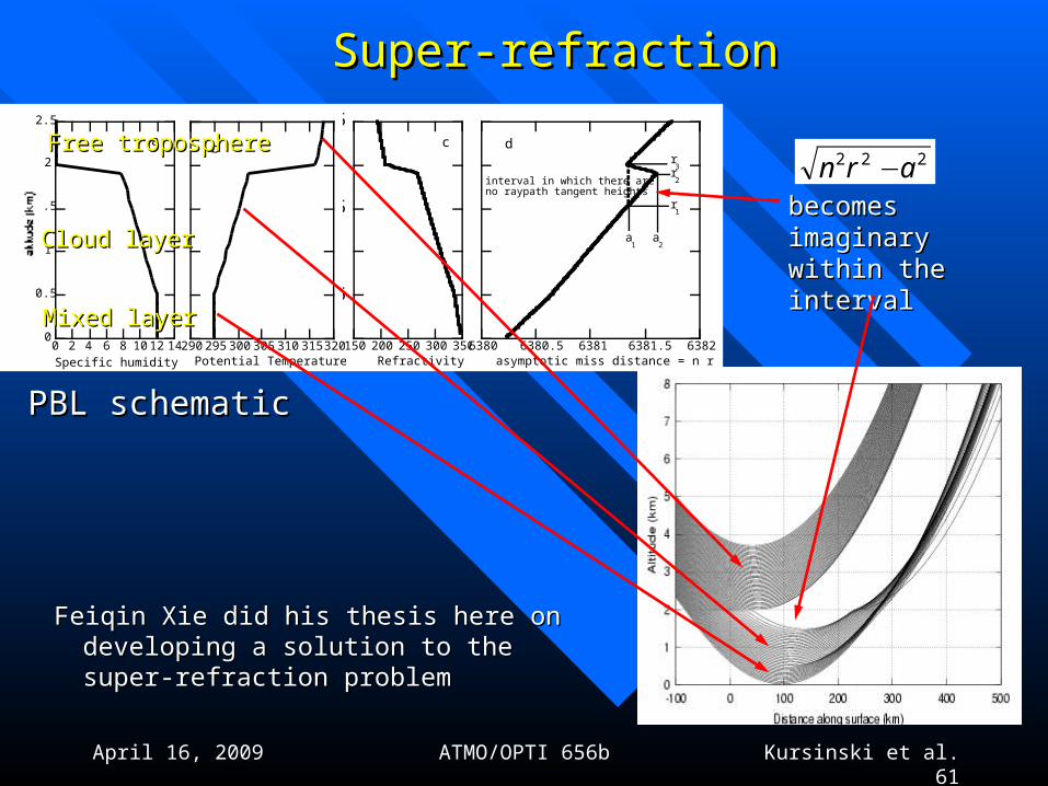
PBL schematicPBL schematic
0 2 4 6 8 10 12 140
0.5
1
1.5
2
2.5
Specific humidity (g/kg)
altitude (km)
a
290 295 300 305 310 315 320Potential Temperature (K)
b
6380 6380.5 6381 6381.5 6382asymptotic miss distance = n r (in km)
interval in which there are no raypath tangent heights
r1
r2
r3
a1
a2
d
150 200 250 300 3500
0.5
1
1.5
2
2.5
Refractivity
c
Super-refractionSuper-refraction
becomes becomes imaginary within imaginary within the intervalthe interval
222 arn −
Feiqin Xie did his thesis here on developing a Feiqin Xie did his thesis here on developing a solution to the super-refraction problemsolution to the super-refraction problem
Free troposphereFree troposphere
Mixed layerMixed layer
Cloud layerCloud layer
April 16, 2009 ATMO/OPTI 656b Kursinski et al. 62
Occultation Features SummaryOccultation Features Summary
Occultation signal is a point source Occultation signal is a point source Fresnel Diffraction limited vertical resolutionFresnel Diffraction limited vertical resolution Very high vertical resolutionVery high vertical resolution
We control the signal strength and therefore have much more We control the signal strength and therefore have much more control over the SNR than passive systemscontrol over the SNR than passive systems
Very high precision at high vertical resolution Very high precision at high vertical resolution
Self calibrating techniqueSelf calibrating technique
Source frequency and amplitude are measured immediately Source frequency and amplitude are measured immediately before or after each occultation so there is no long term driftbefore or after each occultation so there is no long term drift
Very high accuracyVery high accuracy
April 16, 2009 ATMO/OPTI 656b Kursinski et al. 63
Occultation Features SummaryOccultation Features Summary
Simple and direct retrieval concept
Known point source rather than unknown distributed source that must be solved for
Unique relation between variables of interest and observations (unlike passive observations)
Retrievals are independent of models and initial guesses
Height is independent variable
Recovers geopotential height of pressure surfaces remotely completely independent of radiosondes
April 16, 2009 ATMO/OPTI 656b Kursinski et al. 64
Occultation Features SummaryOccultation Features Summary
Microwave system Can see into and below clouds, see cloud base and multiple cloud layers Retrievals only slightly degraded in cloudy conditions Allows all weather global coverage with high accuracy and vertical resolution
Complementary to Passive Sounders
Limb sounding geometry and occultation properties complement passive sounders used operationally