APS MAG Oct 1999

8/13/2019 APS MAG Oct 1999

http://slidepdf.com/reader/full/aps-mag-oct-1999 1/23

Fractal Antenna Engineering: The Theory and

Design of Fractal Antenna Arrays

Douglas H. Werner', Randy L. Haup?,

and Pingjuan L. WerneJ

'Communications and Space Sciences LaboratoryThe Pennsylvania State University

Department of Electrical Engineering

21 1A Electrical E ngineering East

University Park, PA 16802

E-mail: [email protected]

2Department of E lectrical Engineering

Utah State University

Logan, UT 84322-4 120

Tel: (435) 797-2840

Fax: (435) 797-3054

E-mail: [email protected] or [email protected]

3The Pennsylvania State University

College of Engineering

DuBois, PA 15801

E-mail: [email protected]

Keywords: Fractals; antenna arrays; antenna theory; antenna

radiation patterns; frequency-independent antennas; log-periodicantennas; low-sidelobe antennas; array thinning; array signal

processing

1. Abstract

A fractal is a recursively generated object having a fractionaldimension. Many objects, including antennas, can be designed

using the recursive nature of a fractal. In this article, we provide a

comprehensive overview of recent developments in the field of

fractal antenna engineering, with particular emphasis placed o n the

theory and design of fractal arrays. We introduce some important

properties of fractal arrays, including the frequency-independent

multi-band characteristics, schemes for realizing low-sidelobe

designs, systematic approaches to thinning, and the ability to

develop rapid beam-forming algorithms by exploiting the recursive

nature of fractals. These arrays have fractional dimensions that are

found from the generating subarray used to recursively create the

fractal array. Our research is in its infancy, but the results so far are

intriguing, and may have future practical applications.

2. Introduction

he term fructal, which means broken or irregular fragments,T as originally coined by M andelbrot [11 to de scribe a family

of complex shapes that possess an inherent self-similarity in theirgeometrical structure. Since the pioneering work of Mandelbrotand others, a wide variety of applications for fractals has been

found in many branches of science and engineering. One such area

isfructul electrodynamics [2-61, in which fra ctal geome try is com-

bined with electromagnetic theory for the purpose of investigating

a new class of radiation, propagation, and scattering problems. One

of the m ost promising areas of fractal electrodynamics research isin its application to antenna theory and design.

Traditional approaches to the analysis and design of antenna

systems have their foundation in Euclidean geometry. There has

been a considerable amount of recent interest, however, in the pos-

sibility of developing new types of antennas that employ fractal

rather than Euclidean geometric concepts in their design. We refer

to this new and rapidly growing field of research asfructal antenna

engineering. There are primarily two active areas of research in

fractal antenna engineering, which include the study of fractal-

shaped antenna elements, as well as the use of fractals in antenna

arrays. The purpose of this article is to provide an overview ofrecent developments in the theory and design of fractal antenna

arrays.

The first application of fractals to the field of antenna theory

was reported by Kim and Jaggard [7 ] . They introduced a method-

ology for designing low-sidelobe arrays that is based on the theory

of random fractals. The subject of time-harmonic and time-

dependent radiation by bifractal dipole arrays was addressed in [8].

It was shown that, w hereas the time-harmonic far-field response .of

a bifractal array of Hertzian dipoles is also a bifractal, its time-

dependen t far-field response is a unifractal. La &takia et al. [9]

demonstrated that the diffracted field of a self-similar fractal screenalso exhibits self-similarity. This finding was based on results

obtained using a particular example of a fractal screen, constructedfrom a Sierpinski carpet. Diffraction from Sierpinski-carpet aper-

tures has also been considered in [6] , [lo], and [ l l ] . The relatedproblems of diffraction by fractally serrated apertures and Cantor

targets have be en inves tigated in [12-171.

/E€€ ntennas a nd Propagation Magazine, Vol. 41, No. 5,October I999 1045-9243/99/$10.0001999 IEEE 37

mailto:[email protected]








8/13/2019 APS MAG Oct 1999


The fact that self-scaling arrays can produce fractal radiation

patterns was first established in [181. This was accomplished by

studying the properties of a special type of nonuniform linear

array, called a Weierstrass array, which has self-scaling element

spacings and curren t distributions. It was late r shown in [19] how a

synthesis technique could b e developed for Weierstrass arrays that

would yield radiation patterns having a certain desired fractal

dimension. This work was later extended to the case of concentric-

ring arrays by Liang et al. [20]. Applications of fractal concepts tothe design of multi-band Koch arrays, as well as to low-sidelobe

Cantor arrays, are discussed in [21]. A more general fractal geo-

metric interpretation of classical frequency-independent antenna

theory has been offered in [22]. Also introduced in [22] is a design

methodology for multi-band W eierstrass fractal arrays. Other types

of fractal array configurations that have been considered include

planar Sierpinski carpets [23-251 and concentric-ring Cantor arrays

[261.3.1 Cantor linear arrays

t

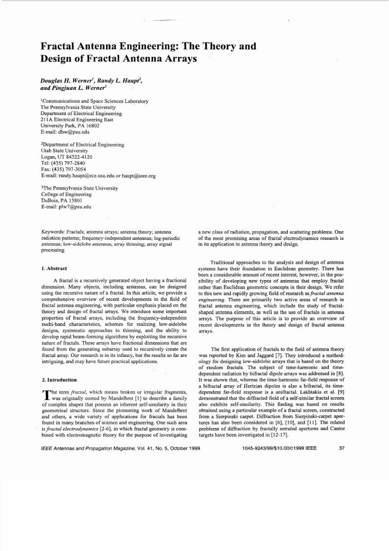
Figure 1. The geom etry for a linear array of uniformly spaced

isotropic sources.

The theoretical foundation for the study of deterministic

h c t a l arrays is developed in Section 3 of this article. In particular,

a specialized pattern-multiplication theorem for fractal arrays is

introduced. Various types of fractal array configuration are also

considered in Section 3, including Cantor linear arrays and

Sierpinski carpet planar arrays. Finally, a more general and sys-tematic approach to the design of deterministic fractal arrays is

outlined in Section 4. This generalized approach is then used to

show that a wide variety of practical array designs may be recur-

sively constructed using a concentric-ring circular subarray gen-erator.

A linear array of isotropic elements, uniformly spaced a dis-

tance d apart along the z axis, is shown in Figure 1. The array fac-

tor corresponding to this linear array may b e expressed in the form

[27,281

3. Deterministic fractal arrays

A rich class of fractal arrays exists that can be formed recur-

sively through the repetitive application of a generating subarray.

A generating subarray is a small array at scale one ( P = 1) used toconstruct larger arrays at higher scales (i.e., P > 1 . In many cases,

the generating subarray has elements that are turned on and off in a

certain pattern. A set formula for copying, scaling, and translationof the generating subarray is then followed in order to produce the

fractal array. Hence, fractal arrays that are created in this manner

will be com posed of a sequence of self-similar subarrays. In other

words, they m ay be conveniently thought of as arrays of arrays [6].

The array factor for a fractal array of this type may be

expresse d in the general form [23-2.51

P

p=l

AF, ( w )=n A( dP- w)7

where GA(y) epresents the array factor associated with the gen-

erating subarray. The parameter 6 is a scale or expansion factor

that governs how large the array grows with each recursive appli-cation of the generating subarray. The expression for the fractal

array factor given in Equation (1) is simply the product of scaled

versions of a generating subarray factor. Therefore, we may regard

Equation (1) as representing a formal statement of the pattern-

multiplication theorem for fractal arrays. Applications of this spe-

cialized pattern-multiplication theorem to the analysis and design

of linear as well as planar fractal arrays will be considered in the

following sections.

where

y = kd [COSBCOS Bo]

and

These arrays become fractal-like when appropriate elements are

turned off or removed, such that

if element n is turned on

if element n is turned off.n {i,Hence, fractal arrays produced by following this procedure belong

to a special category of thinned arrays.

One of the simplest schemes for constructing a fractal linear

array follows the recipe for the Cantor set [29]. Cantor linear arrays

were first proposed and studied in [21] for their potential use in the

design of low-sidelobe arrays. Som e other aspects of Cantor arrays

have been investigated more rec ently in [23-251.

The basic triadic Cantor array may be created by starting with

a three-element generating subarray, and then applying it repeat-

edly over P scales of growth. The generating subarray in this case

has three uniformly spaced elements, with the center element

turned off or removed, i.e., 101. The triadic Cantor array is gener-

ated recursively by replacing 1 by 101 and 0 by 000 at each stage

of the construction. For example, at the second stage of construc-

tion ( P 2 ), the array pattern would look like

38 /€€€Antennas and Propagation Magazine, Vol. 41, No. 5, October 1999

8/13/2019 APS MAG Oct 1999


1 0 1 0 0 0 1 0 1 ,

and at the third stage ( P = 3 ), we would have. . , .

1 0 1 0 0 0 1 0 , 1 0 0 0 0 0 0 0 0 0 1 0 1 0 0 0 1 0 1 .

The array factor of the three-element generating subarray with the

representation 101 is

G A ( v ) = 2 c o s ( y ) , ( 6 )

which m ay be derived from Equation (2) by setting N = 1, I , = 0 ,

and 1, 1 . Substituting Equation (6) into Equation ( I ) and choos-

ing an expansion factor of three (i.e., S = 3) results in an expres-

sion for the C antor array factor given by

-0 .4

-2 -1.5 .l -0.5 0 0.5 1 1.5 2P A

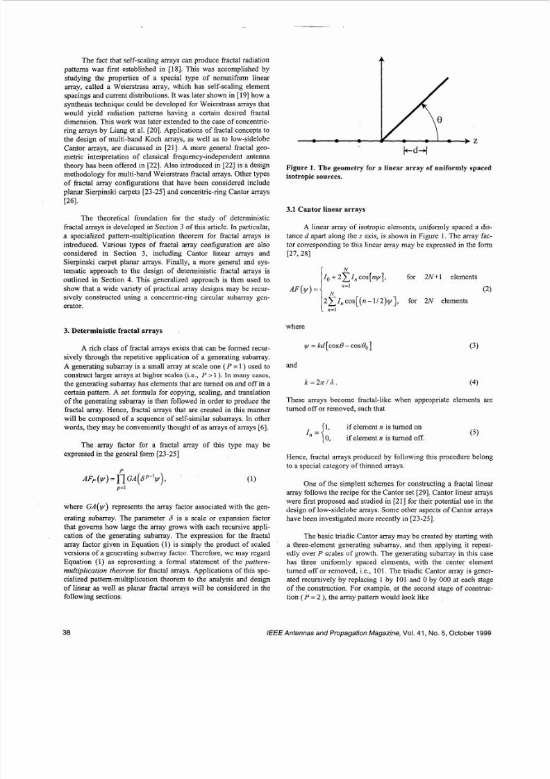
A ( i y ) =n A(3p- 'y ) = i c 0 ~ ( 3 ~ - l i y ) , (7) Figure 2c. A plot of the triadic Cantor fractal array factor for

the th i rd s tage o f g rowth , P = 3 . The array facto r is=l=l

c o s ( ~ ) c o s ( 3 ~ ) c o s ( 9 ~ ) .

1

0 9

0 8

0 7

0 6

0 5

O d

0 3

0 2

0 1

0

-2 - 1 5 - 1 - 0 5 0 0 5 1 1 5 2

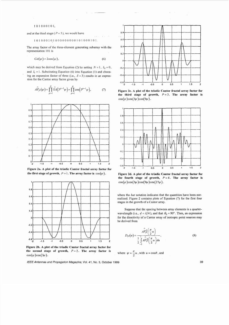
.2 -1.5 -1 -0.5 0 0.5 1 1.5 2Figure 2a. A plot of the triadic Cantor fractal array factor for

the first stage of growth, P = I . The array facto r is c os(y ) . Figure 2d. Azplot of the triadic Cantor fractal array factor for

th e fo u r th st ag e of g row th, P = 4 . T h e a r r ay f ac to r is

cos(v/)cos(3v/)cos(91r/)cos(27ry).

_---- . where the hat notation indicates that the quantities have been nor-malized. Figure 2 contains plots of Equation (7) for the first fourstages in the gro wth of a Ca ntor array.

-- Suppose that the spacing between array elements is a quarter-

wavelength (i.e., d = R / 4 ) , and that Bo = 90 . Then, an expression

for the directivity of a Cantor array of isotropic point sources may

be derived from

-2 -1.5 - 1 -0.5 0 0.5 1 1.5 2

Figure 2b. A plo t o f the t r iad ic Can to r f ractal array facto r fo r

the second stage of growth, P = 2 . The array facto r i s 7Twhere ry = U , with u = c o s @ ,and

c o s ( ~ ) c o s3 4 . 2

IEEE Antennas and Propagation Magazine, Vol. 41, No. 5, October 1999 39

8/13/2019 APS MAG Oct 1999


(9)

Substituting Equation (9) into Equation (8) and using the fact that

~ f @ + c o s ( 3 P - ' n U ) ] d u = I-I p=l

leads to the following convenient representation for the directivity:

p=l / 2

D ~ ( U ) = ~ [ l + c o s ( 3 ~ - ~ ~ u ) ]2 p n c o s 2 3 -',U . (11)p=l

Finally, it is easily demonstrated from Equation (1 1) that the

maxim um value o f directivity for the Cantor array is

D, = D, (0)= 2', where P = 1,2,.. (12)

or

D p (d B )=3 . 0 1 P , w h ere P =1 , 2 .... (13)

Locations o f nulls in the radiation pattern are easy to com pute

from the product form of the array factor, Equation ( 1 ) . Forinstance, at a given scale P , the nulls in the radiation pattern of

Equation (9) occur when

cos[qzu)0

Solving Equation (14) for U yields

U[ = +(2k - )(1/3)'-' , where k = 1,2,. . , 3'-' + 1)/2. (15)

Hence , from this we m ay easily conc lude that the radiation patterns

produced by triadic Cantor arrays will have a total of 3'- + I

nulls.

Th e generating subarray for the triadic C antor array discussed

above is actually a special case of a more general family of uni-form Ca ntor arrays. The generating subarray factor for this general

class of uniform Ca ntor arrays may be expressed in the form

where

S = 2 n + 1 a n d n = l , 2 , ... (17)

Hence, by substituting Equation (16) into Equation (I) , it follows

that these uniform Cantor arrays have fractal array factor repre-sentations given by [21,23-251

For n = I (6 3 ) , the generating subarray has a pattern 101 such

that Equation (18) reduces to the result for the standard triadic

Cantor array found in Equation ( 7 ) . The generating subarray pat-

tern for the next case, in which n = 2 6 5 ), is 10101 and, like-

wise, when n = 3 ( 6 = 7 ) , the array pattern is 1010101.The fractal

dimension D of these uniform Cantor arrays can be calculated as

P I 1

This suggests that D = 0.6309 for n = 1, D = 0.6826 for n = 2 ,

and D = 0.7124 for n = 3 .

As before, if it is assumed that d = /3/4 and 8, = 90°, then the

directivity for these uniform Cantor arrays may be expressed as

[23-251

r

where use has been m ade of the fact that

The correspo nding expression for maxim um directivity is

, where P= l , 2 ,..., ( 2 2 )

zot0 ' . ' ' . ' ' ' '

Theta (degrees)

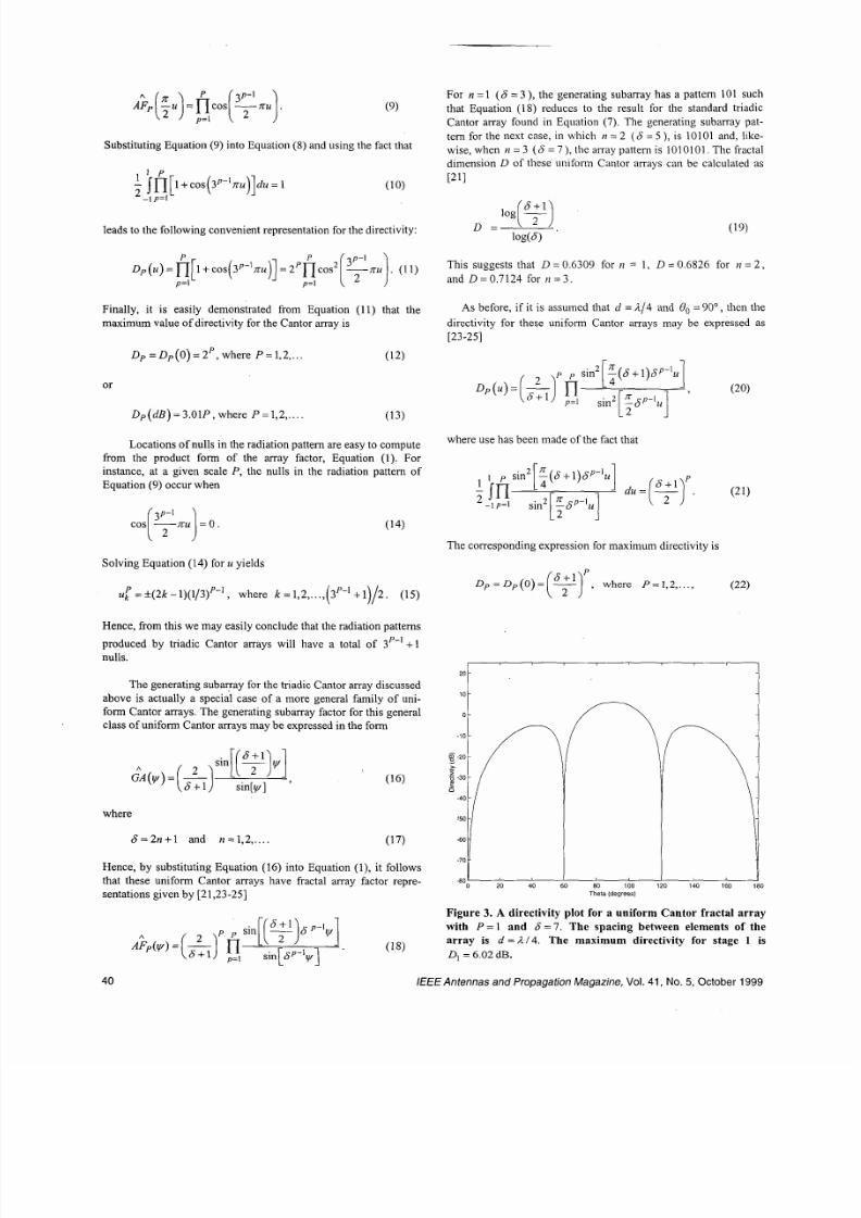
Figure 3. A directivity plot for a uniform Cantor fractal array

with P = l and 6= 7 . The spacing between elements of the

array is d = 1 / 4 . The maximum directivity for stage 1 is

D , = 6.02 dB.

40 /€€€Antennas and Propagation Magazine, Vol. 41, No. 5 , October 1999

8/13/2019 APS MAG Oct 1999


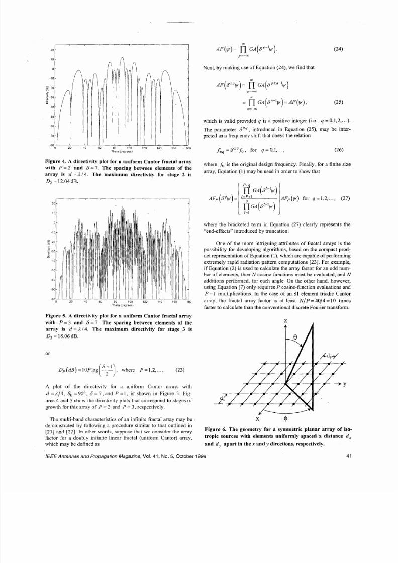
Figure 4. A directivity plot for a uniform Cantor fractal array

with P = 2 and 6 = 7 . The spacing between elements of the

array is d = 1 1 4 . The maximum directivity for stage 2 is

0 2 = 12.04dB.

20

10

-10

g -20->

2 30

-40

-50

-60

-70

20 40 60 80 100 120 140 160 180-80

Theta (degrees)

Figure 5. A directivity plot for a uniform C antor fractal array

with P = 3 and 6 = 7 . The spacing between elements of the

array is d = / 2 / 4 . The maximum directivity for stage 3 is

4 = 18.06 dB.

or

, where P=1 ,2 .... (23)

A plot of the directivity for a uniform Cantor array, with

d = 1 1 4 , 0, = 90°, 6 7 , and P = 1, is' shown in Figure 3. Fig-

ures 4 and 5 show the directivity plots that correspond to stages of

growth for this array of P = 2 and P = 3 , respectively.

The multi-band characteristics of an infinite fractal array may bedemonstrated by following a procedure similar to that outlined in

[21] and [22]. In other words, suppose that we consider the array

factor for a doubly infinite linear fractal (uniform Cantor) array,which may be defined as

p=-m

Next, by making use of Equation (24 ), we find that

n=-m

which is valid provided q is a positive integer (i.e., q = 0,1,2,...).

The parameter 6 4, introduced in Equation (25), may be inter-

preted a s a frequency shift that obeys the relation

where fo s the original design frequency. Finally, for a finite size

array, Equation (1) may be used in order to show that

~

IEEE Antennas and Propagation Magazine, Vol. 41, No. 5, October 1999 41

where the bracketed term in Equation (27) clearly represents the

"end-effects'' introduced by truncation.

One of the more intriguing attributes of fractal arrays is thepossibility for developing algorithms, based on the compact prod-

uct representa tion of Equation ( l) , which are capable of performing

extreme ly rapid radiation pattern computations [23]. For example,

if Equation (2) is used to calculate the array factor for an odd num-

ber of elements, then N cosine functions must be evaluated, and N

additions performed, for each angle. On the other hand, however,

using Equation (7) only requires P cosine-function evaluations and

P - 1 multiplications. In the case of an 81 element triadic Cantor

array, the fractal array factor is at least N I P = 40/4=10 times

faster to ca lculate than the conventional dis crete Fourier transform.

X 4Figure 6. The geometry for a symmetric planar array of iso-

tropic sources with elements uniformly spaced a distance d,

and d, apart in the x and y directions, respectively.

8/13/2019 APS MAG Oct 1999


3.2 Sierpinski carpet arrays

The previous section presented an application of fractal geo-

metric concepts to the analysis and design of thinned linear arrays.

In this section, these techniques are extended to include the more

general case of fractal planar arrays. A symmetric planar array of

isotropic sources, with elements uniformly spaced a distance d,

and d, apart in the x and y directions, respectively, is shown in

Figure 6. It is well known that the array factor for this type of pla-

nar array configuration may be expressed in the following way[28]:

AF(V,?V,) =

where

i 1=2m=2

(28)for ( 2 ~1)2 elements

As before, these arrays can be made fractal-like by following a

systema tic thinning procedure, wh ere

(31)1, if elem ent ( m ,n ) is turned on

0, if element ( m , n ) is turned off1, =

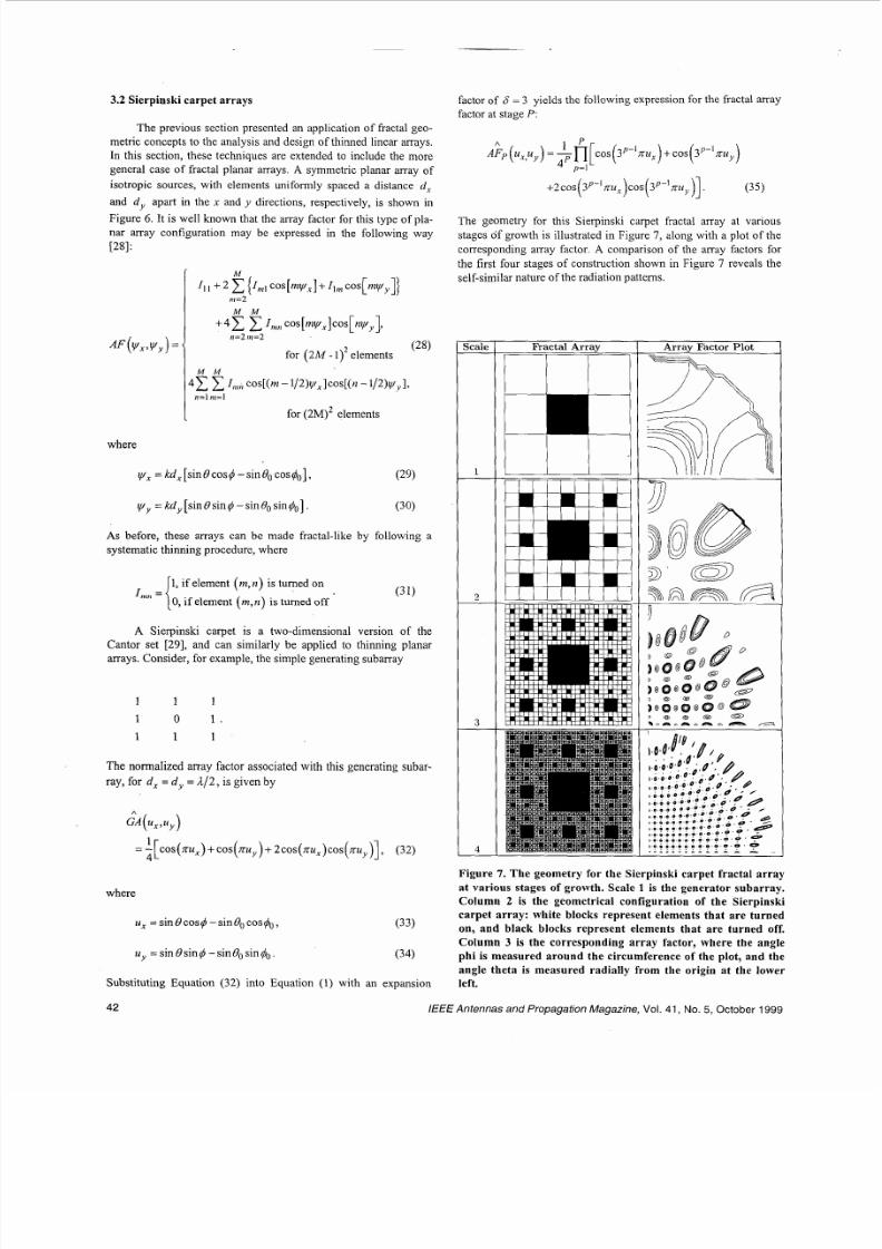
A Sierpinski carpet is a two-dimensional version of theCantor set [29], and can similarly be applied to thinning planararrays. Consider, for exam ple, the simple generating subarray

1 1 1

1 0 1 .

1 1 1

The normalized array factor associated with this generating subar-

ray, for d, = d, = L/2 , is given by

&i, , U,

4= -[cos n u X )+ cos (m y 2 C O S X U , ) cos( U , ] , (32)

where

U, = s in 0 co s4 - ineocos$o, (33)

U , =sin0sinq5-si110~sinq5~. (34)

Substituting Equation (32) into Equation (1) with an expansion

factor of 6 3 yields the follow ing expression for the fractal array

factor at stage P:

A ~ , , ( U , , U ~ )~ ~ [ ~ o s [ 3 ~ ~ ' n r r , ) + c o s ( 3 ~ ~ ' s ~P

p=I

+ 2 c o s ( 3 p - ' s U , ) c o s ( 3 ~ - ' s L ~ y] ( 3 5 )

The geometry for this Sierpinski carpet fractal array at various

stages of growth is illustrated in Figure 7, along with a plot of the

corresponding array factor. A comparison of the array factors for

the first four stages of construction shown in Figure 7 reveals the

self-similar nature of the radiation pattern s.

Scale I Fractal ArravI I I I I

1 l L

L

3

4

l l l l l l l l l l

Arrav Factor Plot

Figure 7. The geometry for the Sierpinski carpet fractal array

at various stages of growth. Scale 1 is the generator subarray.

Column 2 is the geometrical configuration of the Sierpinski

carpet array: white b locks represent elements that are turned

on, and black blocks represent elements that are turned off.

Column 3 is the corresponding array factor, where the angle

phi is m easured around the circumference of the plot, and the

angle theta is measured radially from the origin at the lower

left.

42 /€€€Antennasand Propagation Magazine,Vol. 41, No. 5, October 1999

8/13/2019 APS MAG Oct 1999


An expression for the directivity of the Sierpinski carpet array,

for the case in which Bo = 0 ,may be obtained from

A

where

which follows directly from Equation (35) . The double integral

that appears in the denominator of Equation (36) does not have a

closed-form solution in this case, and therefore must be evaluated

numerically. However, this technique for evaluating the directivity

is much more computationally efficient than the alternative

approach, which involves making use of the Fourier-series repre-

sentation for the Sierpinski carpet array factor given by Equa-

tions (28) and (31), with

yy = n s i n B s i n $ , (39)

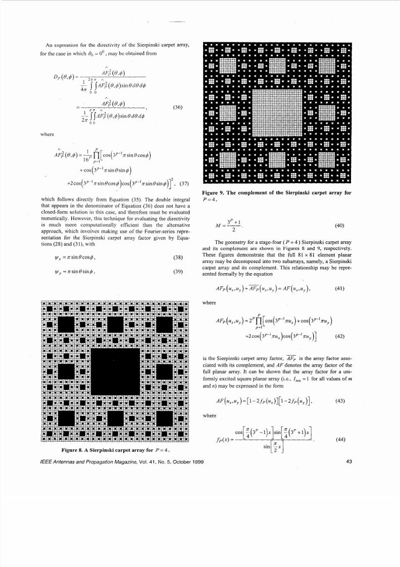
Figure 8. A Sierpinski carpet array for P = 4 .

Figure 9. The complement of the Sierpinski carpet array for

P=4

The geometry for a stage-four ( P = 4) ierpinski carpet arrayand its complement are shown in Figures 8 and 9, respectively.

These figures demonstrate that the full 81 x 81 element planar

array may be decomposed into two subarrays, namely, a Sierpinski

carpet array and its complement. This relationship may be repre-

sented forma lly by the equation

where

AF, (u,,uy) = Yfi[ cos(3p-'7ru,) + cos(3p-'7ruy)p = l

+2cos(3p~ nux)cos(3p~ nuy)] (42)

is the Sierpinski carpet array factor, is the array factor asso-

ciated with its complement, and AF denotes the array factor of the

full planar array. It can be shown that the array factor for a uni-

formly excited square planar array (i.e., I,,,, = 1 for all values of m

and n) may be expressed in the form

where

L L J

IEEE Antennas and Propagation Magazine, Vol. 41 , No. 5 , October 1999 43

8/13/2019 APS MAG Oct 1999


Finally, by using Equation (43) together with Equation (42), an

expression for the complementary array factor % may be

obtained directly from Equation (41). Plots of the directivity for a

P = 4 Sierpinski carpet array and its complement are shown in

Figures 10 and 11, respectively.

The multi-band nature o f the planar Sierpinski carpet arrays may

be easily demonstrated by generalizing the argument presented in

the previous section for linear Cantor arrays. Hence, for doubly

infinite carpets, we have

from which we conclude that

/1F(6'9y,,6'9y,,)= A F ( y , , y , , ) for q = O , I , .... (46)

4. Th e concentric circular ring subarray generator

4.1 Theory

An alternative design methodology for the mathematical con-

struction of fractal arrays will be introduced in this section. The

technique is very general, and consequently provides much more

flexibility in the design of fractal arrays when compared to other

approaches previously considered in the literature [2 1, 23-26]. This

is primarily due to the fact that the generator, in this case, is based

on a concentric circular ring array.

The generating array factor for the concentric circular ring

array may be expressed in the form [30]

ni=l n=l

(47)

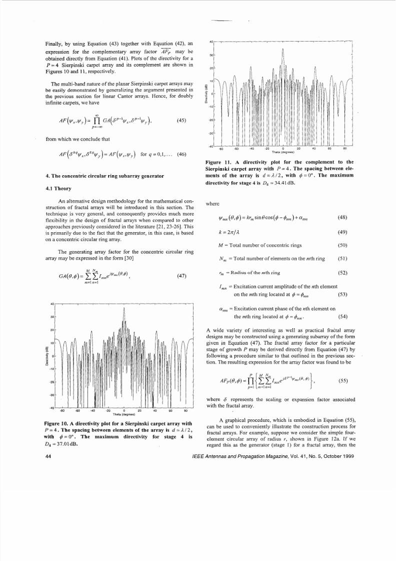
20

10 ig5 0-

-10

-20

-30

-80 -60 .40 -20 0 20 40 60 80-40

Theta (degrees)

Figure 10. A directivity plot for a Sierpinski carpet array with

P = 4 . The spacing between elements of the array is d = A 2 ,

with 4 = O o The maximum directivity for stage 4 is

0 4 = 37.01dB. I;

40

10

-i

=

$ 0

-10

-20

-30

-80 -60-40

-40 -20

Theta (degrees)

0 PO 40 60 80

Figure 11. A directivity plot for the complement to the

Sierpinski carpet array with P = 4 . The spacing between ele-

ments of the array is d = / 2 / 2 , with = O o . The maximum

directivity for stage 4 is D4 34.41 dB.

where

M = Total number of concentric rings ( 5 0 )

Nn , Total number of elements on the mth ring ( 5 1 )

( 5 2 ), =Radius of the mth ring

I,, = Excitation current am plitude of the nth element

on the mth ring located at # = &,,, (53)

a,, = Excitation current phase of the nth element on

the nith ring located at q = 4,,,, . (54)

A wide variety of interesting as well as practical fractal array

designs may be constructed using a generating subarray of the form

given in Equation (47). The fractal array factor for a particular

stage of growth P may be derived directly from Equation (47) by

following a procedure similar to that outlined in the previous sec-

tion. The resulting expression for the array factor was found to be

where 6 represents the scaling or expansion factor associated

with the fractal array.

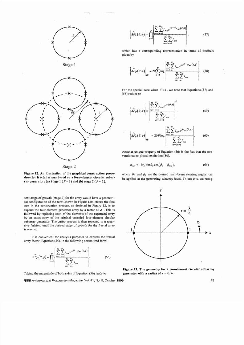
A graphical procedure, which is embodied in Equation (55),

can be used to conveniently illustrate the construction process for

fractal arrays. For exam ple, suppose we consider the simple four-element circular array of radius Y, shown in Figure 12a. If weregard this as the generator (stage 1) for a fractal array, then the

44 /€€€Antennas and Propagation Magazine, Vol. 41, No. 5, October 1999

8/13/2019 APS MAG Oct 1999


Stage 1

Stage 2

Figure 12. An illustration of the graphical construction proce-dure for fractal arrays based on a four-elemen t circular subar-

ray generator: (a) Stage 1 (P 1) and (b) stage 2 (P 2.

next stage of growth (stage 2) for the array would have a geometri-

cal configuration of the form shown in Figure 12b. Hence the first

step in the construction process, as depicted in Figure 12 , is to

expand the four-element generator array by a factor of 6 ,This is

followed by replacing each of the elements of the expanded array

by an exact copy of the original unscaled four-element circular

subarray generator. The entire process is then repeated in a recur-

sive fashion, until the desired stage of growth for the fractal array

is reached.

It is convenient for analysis purposes to express the fractal

array factor, Equation ( 5 5 ) , in the following normalized form:

Taking the magnitude of both sides of Equation ( 5 6 ) eads to

I m= l n = l I

which has a corresponding representation in terms of decibels

given by

For the special case when 6 = 1, we note that Equations ( 5 7 ) and

(58) reduce to

Another unique property of Equation ( 5 6 ) s the fact that the con-

ventional co-phasal excitation [30],

where So and q+ are the desired main-beam steering angles, canbe applied at the generating subarray level. To see this, we recog-

YT+ X

1

Figure 13. Th e geometry for a two-element circular subarray

generator with a radius of r = z 14.

IEEEAntennas and Propagation Magazine, Vol. 41, No.5,October 1999 45

8/13/2019 APS MAG Oct 1999


.-

1 2

cp

1

t

1 3

I cp

cp

3 1

I I

t& 4.

2Stage 1

Y

t

Y A

fcp

1 4 6 4 1

L-h&+I+- - + I t $+I

.

2 2 2

Stage 4

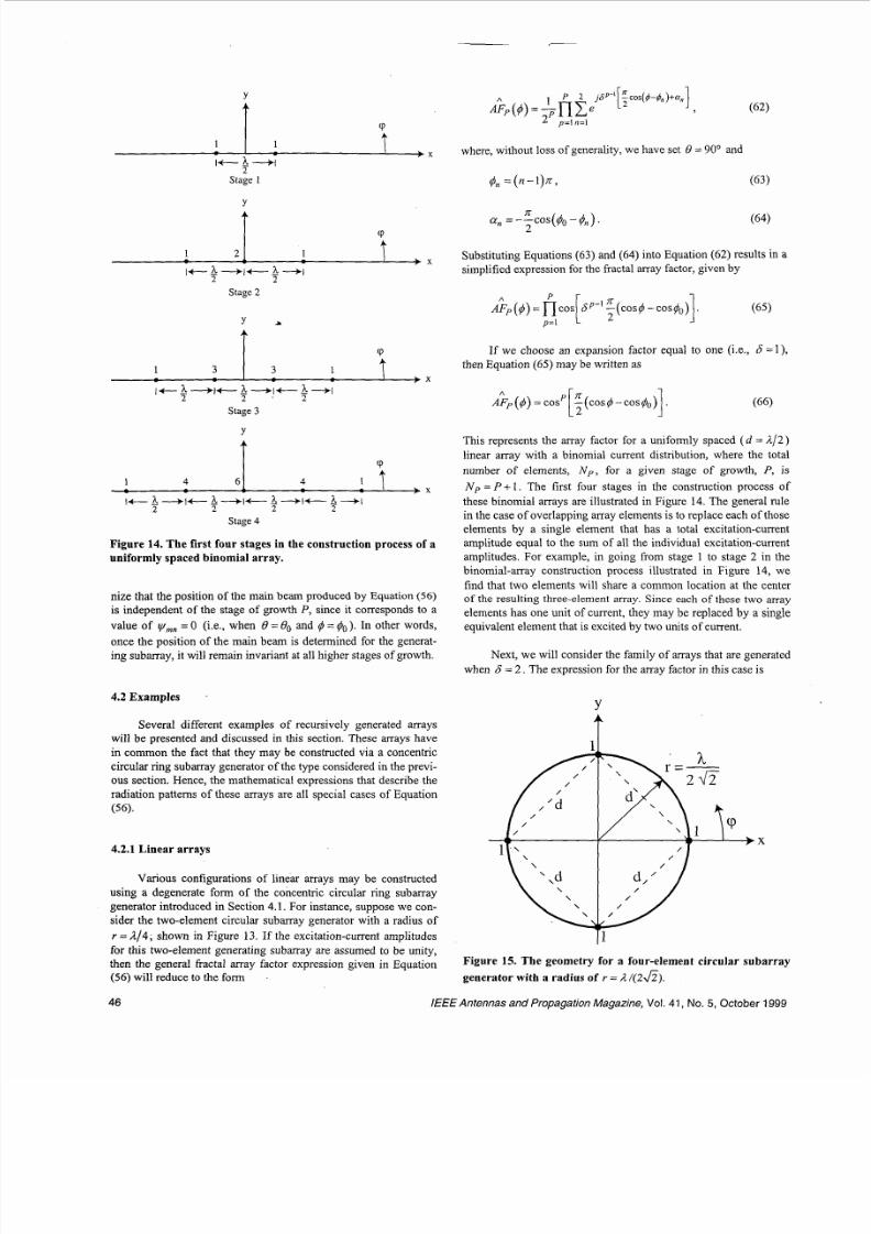
Figure 14. The first four stages in the construction process of a

uniformly spaced binomial array.

nize that the position of the main beam produced by Equation (56)

is independent of the stage of growth P, since it corresponds to a

value of ymn 0 (i.e., when B =So and 4 = q 5 0 . In other words,once the position of the main beam is determined for the generat-

ing subarray, it will rema in invariant at all higher stages of growth.

4.2 Examples

Several different examples of recursively generated arrays

will be presented and discussed in this section. These arrays have

in comm on the fact that they may be constructed via a concentric

circular ring subarray generator of the type considered in the previ-

ous section. Hence, the mathematical expressions that describe the

radiation patterns of these arrays are all special cases of Equation

(56).

4.2.1 Linear arrays

Various configurations of linear arrays may be constructed

using a degenerate form of the concentric circular ring subarray

generator introduced in Section 4.1. For instance, suppose we con-

sider the two-element circular subarray generator with a radius of

Y = L/4; shown in Figure 13 . If the excitation-current amplitudes

for this two-element generating subarray are assumed to be unity,

then the general fractal array factor expression given in Equation(56) will reduce to the form -

where, without loss of generality, we have set 8 = 90 and

Substituting Equations (63) and (64) into Equation (62) results in a

simplified ex pression for the fractal array factor, given by

( 6 5 )p [ ;

;&) = n c o s 6 P - l - (cos+ -COSq50) .p = l

If we choose an expansion factor equal to one (i.e., 6 =1),

then Equation (65) may be written as

> b) = co sp ~ (co s4 -co sq 5 o )

[ 2

This represents the array factor for a uniformly spaced ( d = A / 2 )

linear array with a binomial current distribution, where the total

number of elements, N p , for a given stage of growth, P, is

N p = P + . The first four stages in the construction process of

these binomial arrays are illustrated in Figure 14. The general rule

in the case of overlapping array elements is to replace each of those

elements by a single element that has a total excitation-current

amplitude equal to the sum of all the individual excitation-current

amplitudes. For example, in going from stage 1 to stage 2 in the

binomial-array construction process illustrated in Figure 14, w e

find that two elements will share a com mon location at the centerof the resulting three-element array. Since each of these two array

elements has one unit of c urrent, they may be replaced by a single

equivalent element that is excited by two units of current.

Next, w e will consider the fam ily of arrays that are generated

when 6= 2 . The expression for the array factor in this case is

i

Figure 15. The geometry for a four-element circular subarray

generator with a radius of r = z ?A).

46 IEEE Antennas and Propagation Magazine, Vol. 41, No. 5, October 1999

8/13/2019 APS MAG Oct 1999


Stage 1

.1 *1

'1 '1

Stage 2

*1 *2

2 .4

'1 *2

Stage 3

*1 *3 *3

*3 *9 *9

*3 -9 '9

-1 -3 '3

'2

'1

Stage4

.1 4 '6 *4

'4 '16 '24 '16

.1

-3

*3

(67)A ;p (4 )=n co s=l [ ;p - ~ - ( c o s ~ - c o s ~ o ),

which results from a sequence of uniformly excited, equally spaced

( d = A/2) arrays. Hence, for a given stage of growth P, these

arrays will contain a total of N p =2' elements, spaced a half-

wavelength apart, with uniform current excitations. Finally, the last

case that will be considered in this section corresponds to a choice

of 6 = 3 . This particular choice for the expansion factor gives rise

to the family o f triadic Cantor arrays, which have already been dis-

cussed in Section 3.1. These arrays contain a total of N p = 2

elements, and have current excitations which follow a uniform

distribution. However, the resulting arrays in this case are non-uniformly spaced. This can be interpreted as being the result of athinning process, in which certain elements have been systemati-

cally removed from a uniformly spaced array in accordance with

the standard Cantor construction procedure. The Cantor array fac-tor may be expressed in the form

p [ ;

; p ( 4 ) = n c o s 3 p - ' - ( c o s ~ - c o s ~ o ) ,p=l

which follows directly from Equation (65) when 6 = 3

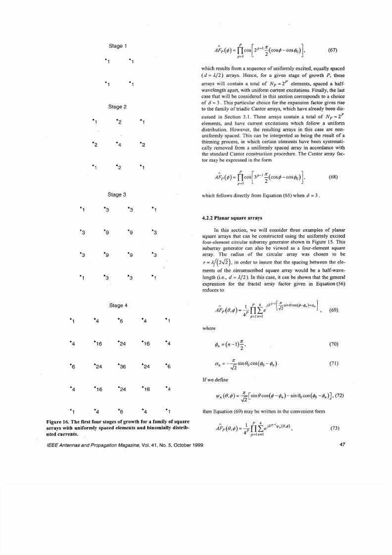
4.2.2 Planar square arrays

In this section, we will consider three examples of planar

square arrays that can be constructed using the uniformly excitedfour-element circular subarray generator shown in Figure 15. This

subarray generator can also be viewed as a four-element square

array. The radius of the circular array was chosen to be

r = A 2 2 , n order to insure that the spacing between the ele-

ments of the circumscribed square array would be a half-wave-

length (i.e., d = A/2). n this case, it can be shown that the general

expression for the fractal array factor given in Equation(56)reduces to

A J

where

7c

4n=(n - I ) - ,2

If we define

*4 '16 24 '16 *4

vn e, = _If_ [ in 0cos(4 -&)- in Bo cos(40 n ] , 72)J5

*4 *6 *4 '1 then Equation (69) may be written in the convenient form

(73)l P 4= - n ~ , j 6 ~ - ' v n ( ~ , b ) ,

Figure 16. The first four stages of growth for a family of squarearrays with uniformly spaced elements and binom ially distrib-

IEEE Antennas and Propagation Magazine, Vol. 41, o. 5,October 1999

uted currents. 4p p=l n=l

47

8/13/2019 APS MAG Oct 1999


where

cCI)

c.-

2 -40.

Now suppose we consider the case where the expansion fac-

tor 6 = 1.Substituting this value of 6 into Equation (73) leads to

The first four stages of growth for this array arc illustrated in Fig-

ure 16. The pattern that emerges clearly shows that this construc-tion process yields a family of square arrays, with uniformly

' spaced elements ( d = /2/2) and binomially distributed currents. For

a given stage of growth P, the corresponding array will have a total

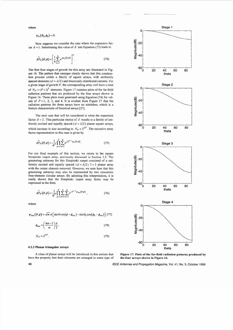
of N p = ( P + elements. Figure 17 contains plots of the far-field

radiation patterns that are produced by the four arrays shown in

Figure 16. These plots were generated using Equation (74) for val-

ues of P = l , 2, 3, and 4. It is evident from Figure 17 that the

radiation patterns for these arrays have no sidelobes, which is afeature characteristic of binomial arrays [27].

The next case that will be considered is when the expansion

factor 6 = 2 . This particular choice of esults in a family of uni-

formly excited and equally spaced ( d = /2/2) planar square arrays,

which increase in size according to N p = 2". The recurs ive array

factor representation in.this case is given by

For our final example of this section, we return to the squareSierpinski carpet array,previously discussed in Section 3.2. The

generating subarray for this Sierpinski carpet consisted of a uni-

formly excited and equally spaced ( d = A / 2 ) 3 x 3 planar array

with the center element removed. However, we note here that thisgenerating subarray may also be represented by two concentric

four-element circular arrays. By adopting this interpretation, it is

easily shown that the Sierpinski carpet array factor may beexpressed in the form

where

N~ = 23p. (79)

4.2.3 Planar triangular arrays

A class of planar arrays will be introduced in this section thathave the property that their elements are arranged in some type of

Stage 1

-600 20 40 60 80

theta

Stage 3

0

g 20

a,

U

c.-g-405

-600 20 40 60 80

theta

Stage 4

-600 20 40 60 80

theta

Figure 17. Plots of the far-field radiation patterns produced bythe four arrays shown in Figure 16.

48 IEEE Antennas and Propagation Magazine, Vol. 41, No. 5,October 1999

8/13/2019 APS MAG Oct 1999


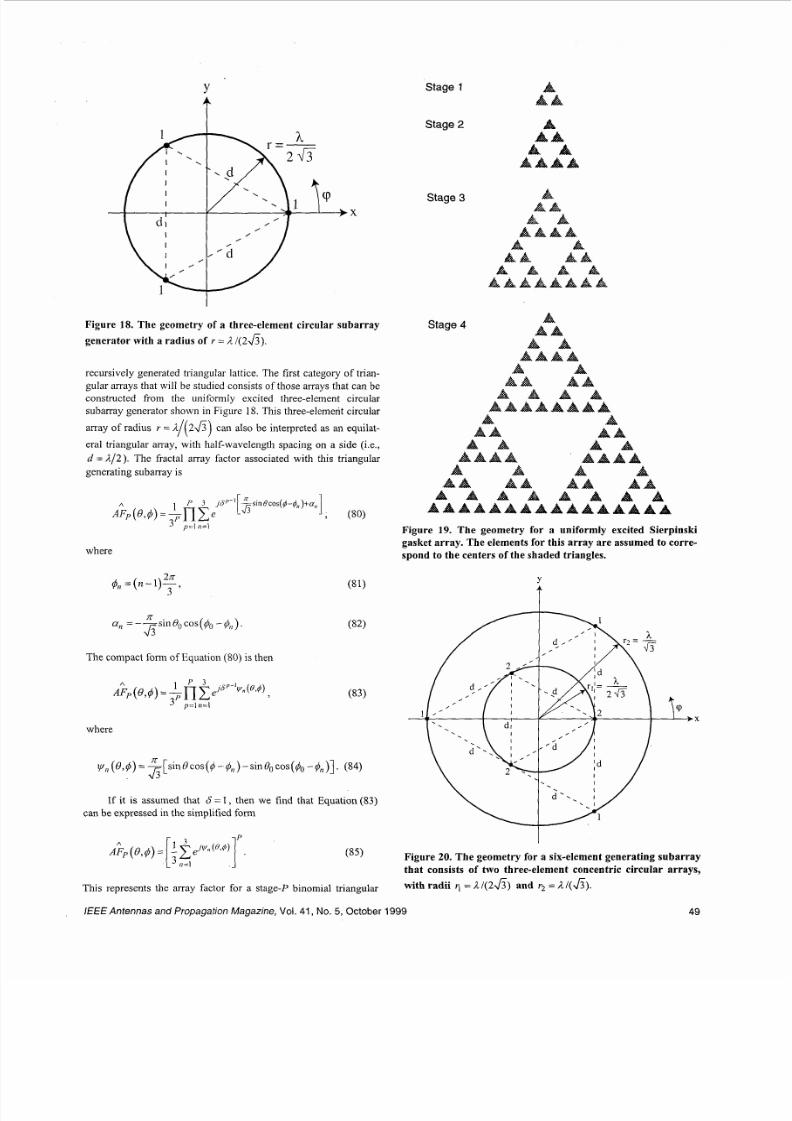
Figure 18. Th e geometry of a three-element circular subarr ay

generato r with a rad ius o f Y = A/(2 ) .

recursively generated triangular lattice. The first category of trian-gular arrays that will be studied c onsists of those arrays that can be

constructed from the uniformly excited three-element circular

subarray generator shown in Figure 18. This three-element circular

array of radius Y = A/( 2&) can also be interpreted as an equilat-

eral triangular array, with half-wavelength spacing on a side (i.e.,

d = A / 2 ) . The fractal array factor associated with this triangular

generating subarray is

p=l,,=I

where

2z

3(II,=(E-')--.

an - -s1n~~cos(4 , , -#,,).

J

The compact form of Equation (80) is then

where

If it is assumed that 6 I , then we find that Equation(83)

can be expressed in the simplified form

85)

This represents the array factor for a stage? binomial triangular

Stage 1

Stage 2

Stage 3

Figure 19. The geometry for a uniformly excited Sierpinski

gasket array . Th e elements fo r th is arr ay are assumed to corre-

spond to the cente rs of the shaded triangles.

F ig u re 20. Th e geometry fo r a s ix -element generat ing suba rray

that consists of two three-element concentric circular arrays,

with radii r, = A/(2 ) a n d r2 = A/( ).

/€€€Antennas and Propagation Magazine, Vol. 41, No. 5, October 1999 49

8/13/2019 APS MAG Oct 1999


Stage 3

Stage 1

Stage 2

Stage 4

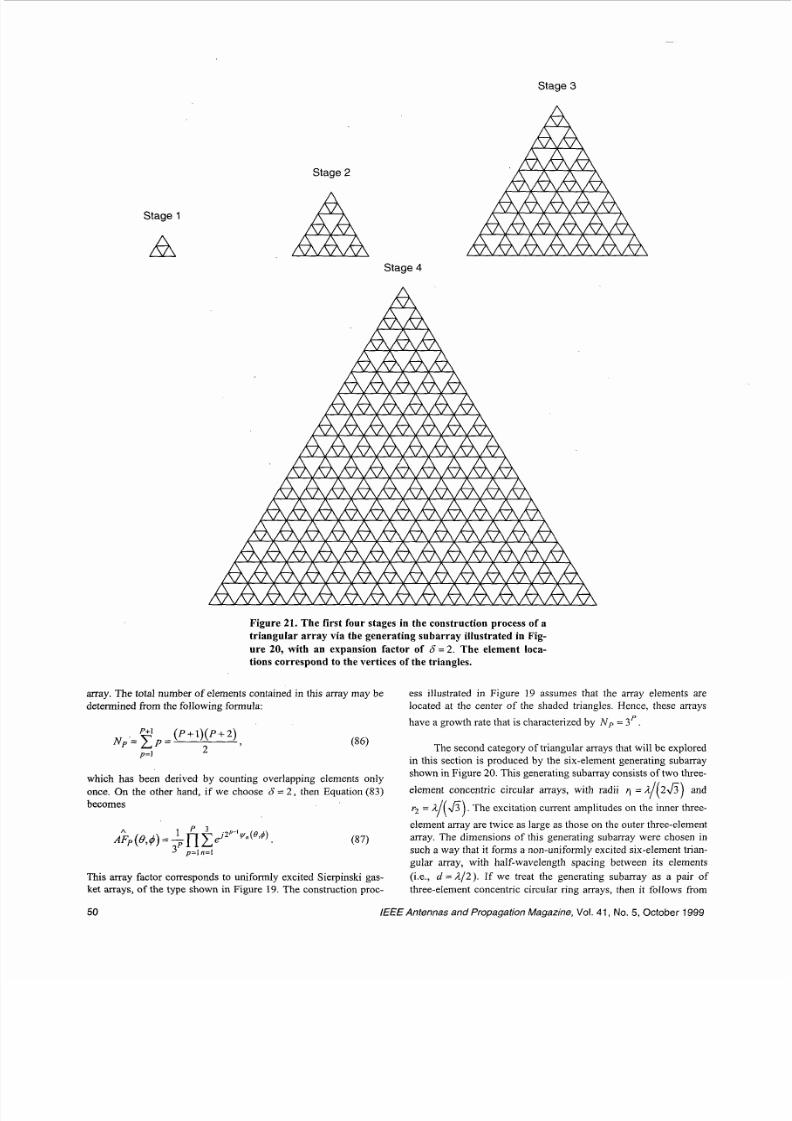
Figure 21. The first four stages in the construction process of a

triangular array via the generating subarray illustrated in Fig-

ure 20, with an expansion factor of 6 = 2 . The element loca-

tions correspond to the vertices of the triangles.

array. The total number of elements contained in this array may be

determined from the following formula:

ess illustrated in Figure 19 assumes that the array elements are

located at the center of the shaded triangles. Hence, these arrays

have a growth rate that is characterized by N P = 3'.

p+l ( P + l ) ( P + 2 )N p . = c p = -I

p=lL

which has been derived by counting overlapping elements only

once. On the other hand, if we choose 6 = 2 , then Equation (83)

becomes

This array factor corresponds to uniformly excited Sierpinski gas-ket arrays, of the type shown in Figure 19. The construction proc-

The second category of triangular arrays that will be explored

in this section is produced by the six-element generating subarray

shown in Figure 20 . This generating subarray c onsists of two three-

element concentric circular arrays, with radii r = d 2 3

r2 = d/(6 .he excitation current amplitudes on the inner three-

element array are twice as large as those on the outer three-element

array. The dimensions of this generating subarray were chosen in

such a way that it forms a non-uniformly excited six-element tnan-gular array, with half-wavelength spacing between its elements

(i.e., d = d/2) . If we treat the generating subarray as a pair of

three-element concentric circular ring arrays, then it follows from

/( J nd

50 IEEEAntennas and Propagation Magazine, Vol. 41, No. 5,October 1999

8/13/2019 APS MAG Oct 1999


8/13/2019 APS MAG Oct 1999


Stage 1 YO r

-600 20 40 60 80

theta

t

Stage 2

Figure 25. The geometry for a uniformly excited six-element

circular subarray generator of radius r = ;1/2.

-60 10 20 40 60 80

theta

Stage 3

-60'0 20 40 60 80

theta

Stage 4

0

isg 20a,m

z0

c.-

(d -40H

-6020 40 60 80

theta

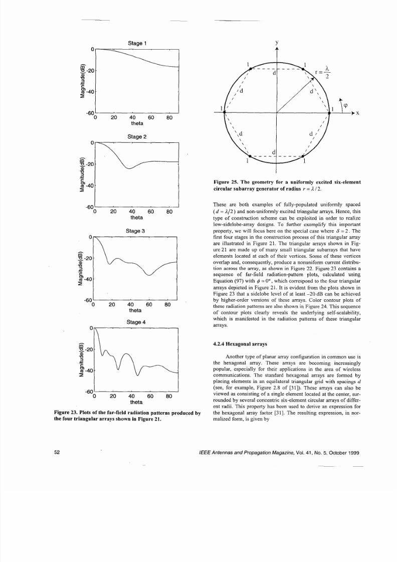
Figure 23. Plots of the far- field radiation patterns produced by

the four triangular arrays show n in Figure 21.

These are both examples of fully-populated uniformly spaced

( d = ;1/2) and non-uniformly excited triangular arrays. He nce, this

type of construction scheme can be exploited in order to realize

low-sidelobe-array designs. To further exemplify this important

property, we will focus here on the special case where 6 = 2 . The

first four stages in the construction process of this triangular a rray

are illustrated in Figure 21 . The triangular arrays shown in Fig-

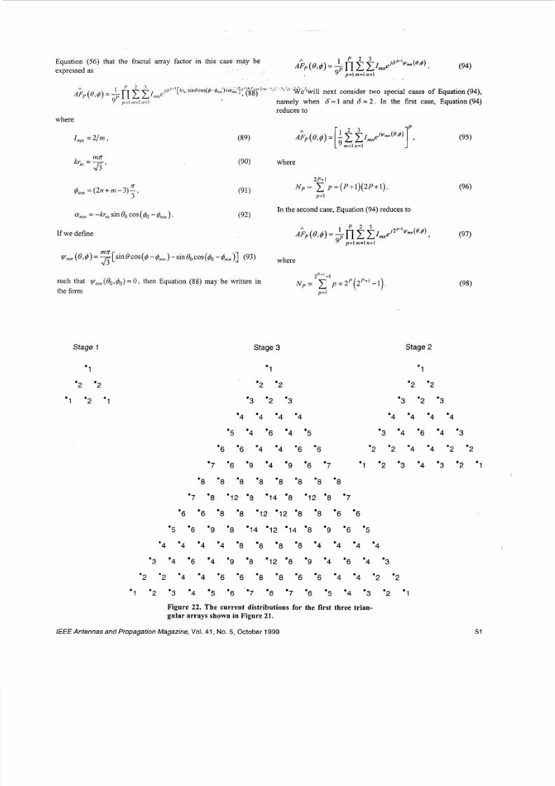
ure 21 are made up of many small triangular subarrays that have

elements located at each of their vertices. Some of these vertices

overlap and, consequently, produce a nonuniform current distribu-tion across the array, as shown in Figure 22. Figure 23 contains a

sequence of far-field radiation-pattern plots, calculated using

Equation (97) with q5 = 0 ,which correspond to the four triangular

arrays depicted in Figure 21 . It is evident from the plots shown in

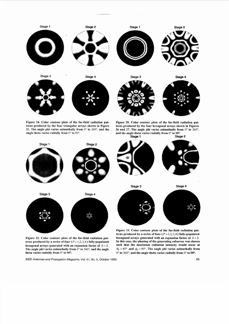
Figure 23 that a sidelobe level of at least -20 dB can be achievedby higher-order versions of these arrays. Color contour plots of

these radiation patterns are also show n in Figure 24. This sequence

of contour plots clearly reveals the underlying self-scalability,

which is manifested in the radiation patterns of these triangulararrays.

4.2.4 Hexagonal arrays

Another type of planar array configuration in comm on use is

the hexagonal array. These arrays are becoming increasinglypopular, especially for their applications in the area of wireless

communications. The standard hexagonal arrays are formed byplacing elements in an equilateral triangular grid with spacings d

(see, for example, Figure 2.8 of [31]). These arrays can also be

viewed as consisting of a single element located at the center, sur-

rounded by se veral concentric six-element circular arrays of differ-

ent radii, This property has been used to derive an expression forthe hexagonal array factor [31]. The resulting expression, in nor-

malized form, is given by

52 IEEE Antennas and Propagation Magazine, Vol. 41, No. 5, October 1999

__

8/13/2019 APS MAG Oct 1999


Stage 1 Stage 2 Stage I Stage 2

Stage 3 Stage4 Stage 3 Stage4

Figure 24. Color c ontour plots of the far-field radiation pa t-

terns produced by the four triangular arrays shown in Figure

21. The angle phi varies azimuthally from 0 to 360", and the ,

angle theta varies radially from 0 to 90 .

Figure 29. Color contour plots of the far-field radiation pat-

terns produced by the four hexagonal arra ys shown in Figures26 and 27. The angle phi varies azimuthally from 0 to 360",

and the angle theta varies radially from 0 to 90 .

Stage 1 Stage 2

Stage 1

Stage 3

Stage 3 Stage 4

Stage 4


terns produced by a series of four ( P 1,2,3,4) fully-populated


terns produced by a series of four ( P 1,2,3,4) fully-populated

hexagonal a rra ys generated with an expansion factor of = 2.

The angle phi varies azimuthally from 0 to 360", and the angle

theta varies radially from 0 to 90 .

hexagonal a rrays generated with an expansion factor of = 2.In this case, the phasing of the genera ting subarray was chosensuch that the maximum radiation intensity would occur at

60 = 45 an d 40= 90". Th e angle phi varies azimuthally from

0 to 360", and the angle theta varies radially from 0 to 90°.

IEEE Antennas and Propagation Magazine, Vol. 41 , No. 5, October 1999 53

8/13/2019 APS MAG Oct 1999


Stage 1

0

Stage 2 Stage 4

Stage 3

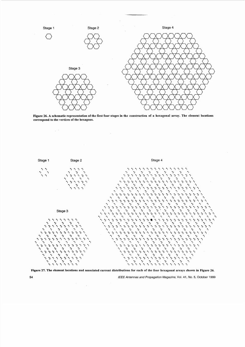
Figure 26. A schematic representationof the first four stages in the construction of a hexagonal array. The element locationscorrespond to the vertices of the hexagons.

Stage 1 Stage 2

.1 'I *l1 1 1

-1 '1 '1 -1

*1 'I '1 2 '1 ' 4'1 'I '1 '1

'I '2 'I -1 '2 'I

1 2 '

-1 *1 -1 -1

Stage 3

Stage 4

*1 -1 *1 *1 *1 *I *I 1 1 *I *I *I -1 *I '1 1

'1 '2 '2 '2 2 '2 '2 -1

-1 '2 -1 -1 3 3 -1 -1 3 3 -1 '1 3 -3 -1 ' '2 '1

-1 -1 2 '2 '2 2 '2 -1 -1

'1 -2 *3 '2 -1 3 3 *I 3 '5 '5 3 -1 3 3 1 '2 3 '2 -1

-1 2 '1 2 3 '2 *1 '1 3 '5 3 3 3 '1 *I '2 3 '2 -1 '2 *I

*1 '1 -1 1 '2 *2, 2 '2 *I '1 -1 -1

*I '2 3 '2 3 4 3 '1 3 '5 3 3 '5 3 *1 '2 3 '4 3 2 3 2 *1

-1 -1 3 3 3 3 '2 '2 3 3 3 3 *I *1

'1 3 3 3 '5 '5 3 '2 3 '5 3 3 3 1

-1 '2 -1 '2 3 -2 -1 2 3 4 3 '2 3 '2 '1 -1 '2 3 2 3 4 3 '2 -1 3 '2 *I '2 '1.

'1 '1 q *I -1 '1 *I 1 '1 '1 '1 '1 *I '1 '1 '1

-1 -2 -1 2 3 2 *1 -2 3 4 3 '2 3 *1 '1 '2 3 '2 3 '4 3 '2 '1 3 '2 *I '2 -1

'1 3 3 '5 '5 3 :2 3 '5 3 3 3 *I

-1 '1 3 3 3 3 2 '2 3 3 3 3 *1 -1

'1 3 3 '2 '4 6 4 '2 3 3 '1

*I 3 3 '4 '6 4 3 5 '1

*1 '2 -1 -2 '6 3 '2 '5 4 *1 3 '5 '5 3 *1 4 '5 3 6 '5 '2 -1 '2 *1

'1 '2 3 '2 '1 4 '5 '2 3 '6 5 '2 '1 3 3 '1 2 5 6 3 '2 5 '4 '1 '2 3 2 '1

'1 '2 3 2 ' 4 '5 '2 3 '6 '5 '2 -1 3 3 '1 '2 '5 '6 3 '2 '5 4 '1 '2 3 '2 '1

1 '2 1 '2 '6 3 '2 4 '1 3 '5 '5 3 '1 '4 '5 '2 3 '6 '2 *I '2 '1-1 3 '5 3 4 '6 '4 3 '5 3 '1

'1 '2 3 '2 3 4 '1 3 3 3 3 1 '2 3 '4 3 '2 3 2 *I

*1 '1 ' -1 '2 '2 '2 -2 4 -1 '1 -1

*1 2 '1 3 2 '1 -1 3 3 '5 3 -1 -1 '2 3 -2 '1 -1

-1 2 3 '2 '1 3 3 1 3 5 3 '1 3 3 -1 '2 3 -2 -1

-1 '1 '2 '2 '2 2 -1 1

-1 2 '1 '1 3 3 *1 '1 3 3 *1 ' 3 3 '1 -1 2 -1

*1 '2 2 '2 2 '2 2 '1

1 1 -1 *1 'I 1 -1 *I -1 '1 '1 *I -1 *I -1 -1

*I 3 3 '2 '4 4 2 3 3 '1

Figure 27. The element locations and associated current distributions for each of the four hexagonal arrays shown in Figure 26.

IEEE Antennas and Propagation Magazine,Vol. 41, No. 5 , October 19994

8/13/2019 APS MAG Oct 1999


8/13/2019 APS MAG Oct 1999


Stage 1

=K

z -40.

r

Stage 1

-6020 40 60 80

Theta (Degrees)

Stage 2

-60 I0 20 40 60 80

Theta (Degrees)

Stage 3

WU

t

H

0 20 40 60 80

Theta (Degrees)

0

iss 20WU

c

.-9 40H

Stage 4

-600 20 40 60 80

Theta (Degrees)

Stage 2

Theta (Degrees)

Stage 3

Theta (Degrees)

Stage 4

O 7

20a,U

Kc

.-2 40

-600 20 40 60 80

Theta (Degrees)

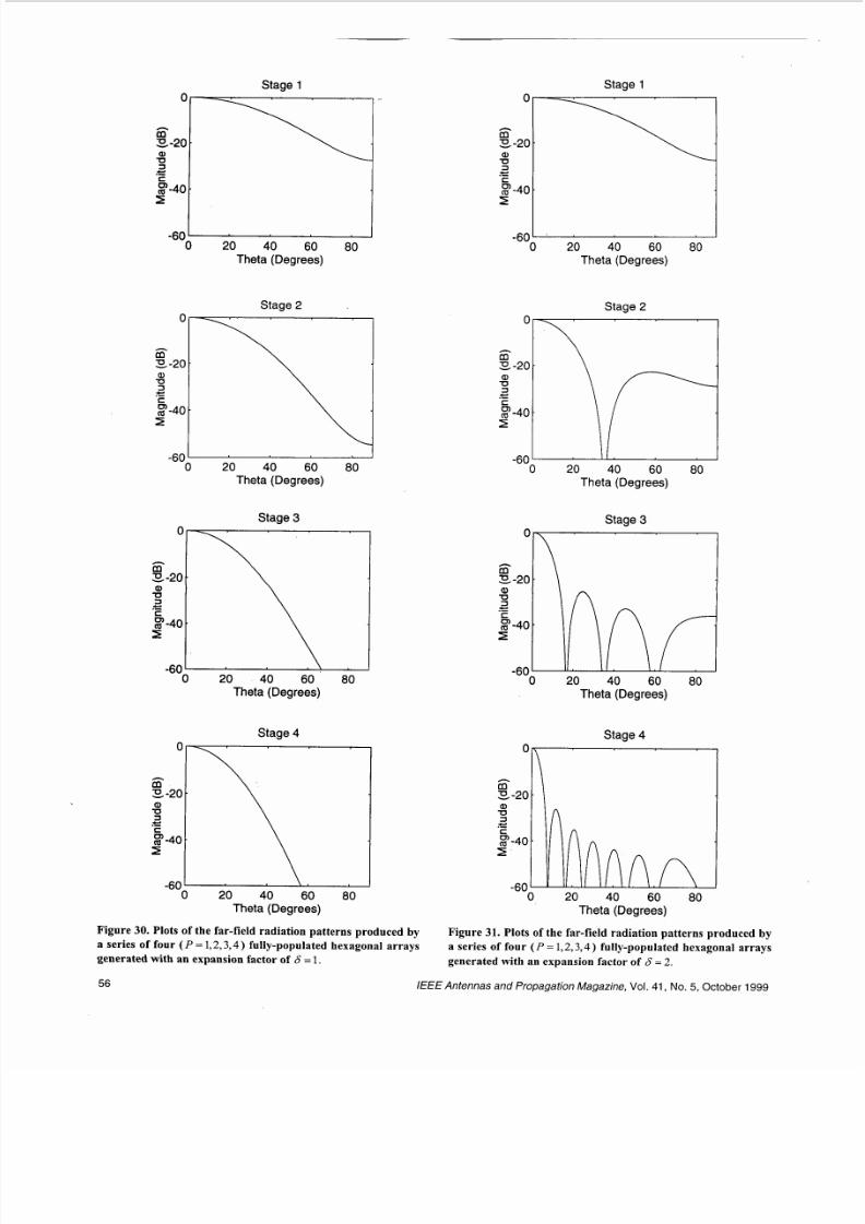
Figure 30. Plots of the far-field radiation patterns produced by

a series of four ( P = 1,2 ,3 ,4) fully-populated hexagonal arrays

generated with an ex pansion factor of 6 = 1.

56

Figure 31. Plots of the far-field radiation patterns produced by

a series of four ( P = 1,2 ,3 ,4) fully-populated hexagonal arrays

generated with an expan sion factor of 6 = 2.

/€€€Antennas and Propagation Magazine, Vol. 4 1, No. 5, October 1999

8/13/2019 APS MAG Oct 1999


These arrays increase in size at a rate that obeys the relationship

Np = 3 P ( P + I ) + (1 - 6 p , ) ,

where 6,, epresen ts the Kronecker de lta function, defined by

1, P = l

0, P # l ’

Pl =

In other words, every time this fractal array evolves from one stage

to the next, the number of concentric hexagonal subarrays con-

tained in it increases by one.

The second special case of interest to be considered in this

section results when a choice of 6 = 2 is made. Substituting this

value of 6 into Equation (107) yields an expression for the recur-

sive hexagonal array factor given by

p = l n = l

where

Clearly, by comparing Equation (1 13) with Equation (1 lo ), we

conclude that these recursive arrays will grow at a much faster rate

than those generated by a choice of 6 = 1. Schematic representa-

tions of the first four stages in the construction process of thesearrays are illustrated in Figure 26, where the element locations cor-

respond to the vertices of the hexagons. Figure 27 shows the ele-

ment locations and associated current distributions for each of thefour hexagonal arrays depicted in Figure 26. Figures26 and 27

indicate that the hexagonal arrays that result from the recursive

construction process with 6 = 2 have some elements missing, i.e.,

they are thinned. This is a potential advantage o f these arrays fromthe design point of view, since they may be realized with fewer

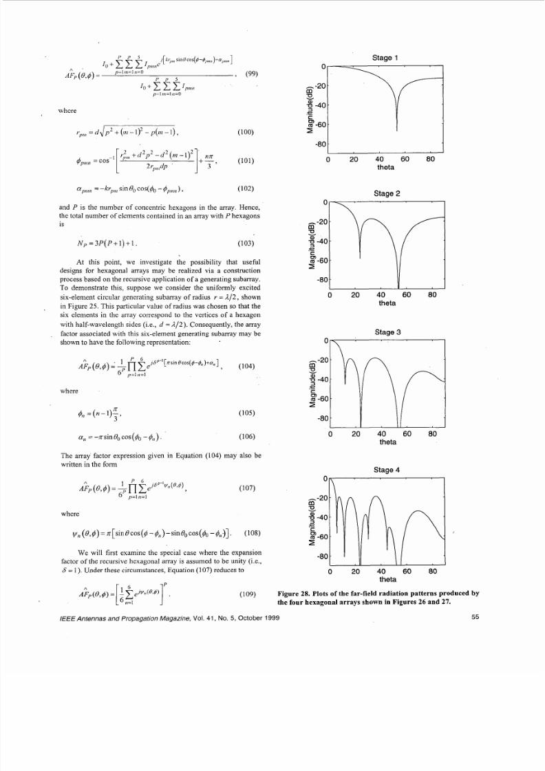
elements. Another advantage of these arrays are that they possess

low sidelobe levels, as indicated by the set of radiation pattern

slices for q5 = 9 0 ” , shown in Figure 28. Full color contour plots of

these radiation patterns have also been included in Figure 29.

Finally, we note that the compact product form of the array factor

given in Equation (112) offers a significant advantage in terms of

computational efficiency, when compared to the conventional hex-agonal array factor representation of Equation (99), especially for

large arrays. This is a direct consequence of the recursive nature of

these arrays, and may be exploited to develop rapid beam-forming

algorithms.

It is interesting to look at what happens to these arrays when

an element with two units of current is added to the center of thehexagonal generating subarray shown in Figure 25. Under thesecircumstances, the expression for the array factor given in Equa-

tion (107) must be modified in the following way:

Plots o f several radiation patterns c alculated from Equation (1 14)

with 6 = 1 and 6 2 are shown in Figures 30 and 3 1, respectively.

These plots indicate that a further reduction in sidelobe levels may

be achieved by including a central element in the generating subar-

ray of Figure 25. Figure 32 contains a series of color contour plotsthat show how the radiation pattern intensity evolves for a choice

of 6 2 . Finally, a series of color contour plots of the radiation

intensity for this array are shown in Figure 33, where the phasing

of the generating subarray has been chosen so as to produce a

main-beam maximum at 19,= 45” and q5 = 9 0 ” .

5. Conclusions

Fractal antenna engineering represents a relatively new field

of research that combines attributes of fractal geometry with

antenna theory. Research in this area has recently yielded a richclass of new designs for antenna elements as well as arrays. The

overall objective of this article has been to develop the theoretical

foundation required for the analysis and design of fractal arrays. It

has been demonstrated here that there are several desirable proper-

ties of fractal arrays, including frequency-independent multi-band

behavior, schemes for realizing low-sidelobe designs, systematic

approaches to thinning, and the ability to develop rapid beam-

forming algorith ms by exploiting the recursive nature of fractals.

6. Acknowledgments

The authors gratefully acknowledge the assistance provided

by Waroth Kuhirun, David Jones, and Rodney Martin.

7. References

1 . B. B. M andelbrot, The Fractal Geo me ty of Nature, New Y ork,

W. H. Freeman, 1983.

2. D. L. Jaggard, “On Fractal Electrodynamics,” in H. N. Kritikos

and D. L. Jaggard (eds.), Recent Advances in ElectromagneticTheory, New York, Springer-Verlag, 1990, pp. 183-224.

3. D. L. Jaggard, “Fractal Electrodynamics and Modeling,” in H. L.Bertoni and L. B. Felson (eds.), Directions in Electromagnetic

Wave Modeling, New York, Plenum Publishing Co., 1991, pp.

435-446.

4. D. L. Jaggard, “Fractal Electrodynamics: Wave InteractionsWith Discretely Self-similar Structures,” in C. Baum and H.

Kritikos (eds.), Electromagnetic Symmetry, Washington DC,

Taylor and Fra ncis Publishers , 1995, pp. 231-281.

5. D. H. Werner, “An Overview of Fractal Electrodynamics

Research,” in Proceedings of the 11th Annual Review of Progress

in Applied Computational Electromagnetics (ACES), Volume II,

(Naval Postgraduate School, Monterey, CA, March, 1995), pp.

964-969.

6. D. L. Jaggard, “Fractal Electrodynamics: From Super Antennasto Superlattices,” in J. L. Vehel, E. Lutton, and C. Tricot (eds.),

Fractals in Engineering, New York, Springer-Verlag, 1997, pp.

204-221.

7. Y. Kim and D. L. Jaggard, “The Fractal Random Array,” Pro-

ceedings of the IEEE, 74, 9, 1986, pp.1278-1280. ,

/€€€Antennas and Propagation Magazine, Vol. 41, No. 5, October 1999 57

8/13/2019 APS MAG Oct 1999


8/13/2019 APS MAG Oct 1999


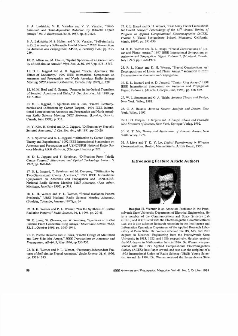
Univ ersity Applied Rese arch Laboratory Outstanding PublicationAward. He has also received several Letters of Commendation

fiom the Pennsylvania State University Department of ElectricalEng ine eri ng for outstanding teach ing and research. Dr.;:Werner is

an Associate Editor of Radio Science, a Senior Member of theIEEE, a member of the American Geophysical Union,

USNCAJRSI Commissions B and G, the Applied Computational

Electromagnetics Society (ACES), Eta Kappa Nu, Tau Beta Pi, and

Sigma Xi. He has published numerous technical papers and pro-ceedings articles, and is the author of six book chapters. His

research interests include theoretical and computational electro-magnetics with applications to antenna theory and design, micro-

waves, wireless and personal communication systems, electromag-

netic wave interactions with complex materials, fractal and knot

electrodynamics, and genetic algorithms.

Randy Haupt is Professor and Department Head in the

Electrical and Computer Engineeiing Department at Utah StateUniversity, Logan, Utah. He has a PhD in Electrical Engineering

from the University of Michigan, an M S in Electrical Engineering

from Northeastern University, an MS in Engineering Managementfrom Western New England College, and a BS in Electrical Engi-

neering from the USAF Academy. Dr. Haupt was a project engi-neer for the OTH-B radar and a research antenna engineer for

Rome Air Development Center. Prior to coming to Utah State, hewas Chair and a Professor in the Electrical Engineering Depart-ment of the University of Nevada, Reno, and a Professor of Elec-

trical Engineering at the USAF Academy. His research interestsinclude genetic algorithms, antennas, radar, numerical methods,signal processing, fractals, and chaos. He was the Federal Engineer

of the Year in 1993, and is a member of Tau Beta Pi, Eta Kappa

Nu, USNCKJRSI Commission B, and the Electromagnetics Acad-

emy. He has eight patents, and is co-author of the book Practical

Genetic Algorithms (John Wiley & Sons, January 1998).

Pingjuan L. Werner received her PhD degree from Perm

State University in 1991. She is currently an Associate Professorwith the College o f Engineering, Penn State. Her research interests

include antennas, wave propagation, genetic-algorithm applicationsin electromagnetics, and fractal electrodynamics. She is a member

of the IEEE, Eta Kappa Nu, Tau Beta Pi, and Sigm a Xi. .E’

11111111111111111111lllllllllllllllllllllllllllllllllllllllllllllllllllllllll

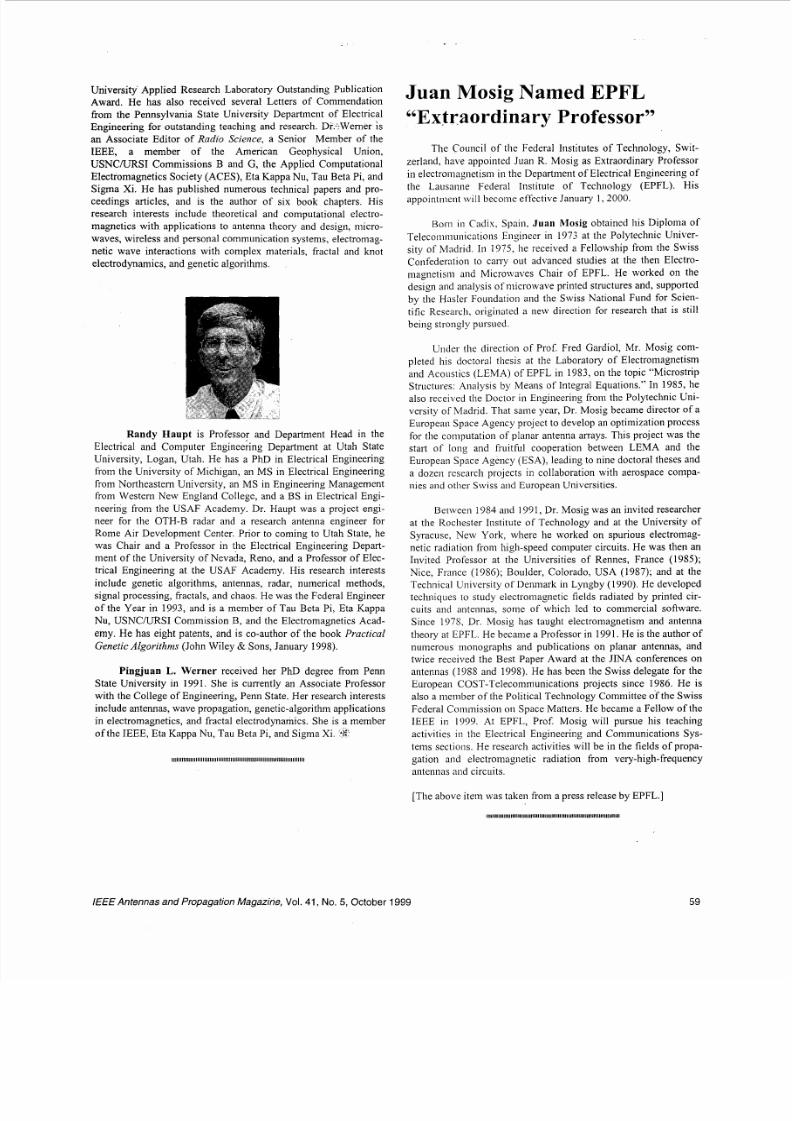
Juan Mosig Named EPFL

“Extraordinary Professor”

The Council of the Federal Institutes of Technology, Swit-

zerland, have appointed Juan R. Mosig as Extraordinary Professor

i n electromagnetism in the Department of Electrical Engineering of

the Lausanne Federal Institute of Technology (EPFL). Hisappointment \vi11 become effective January I , 2000.

Born i n Cadix, Spain, Juan Rlosig obtained his Diploma of

Telecommunications Engineer i n 1973 at the Polytechnic Univer-sity of Madrid. In 1975, he received a Fellowship from the Swiss

Confederation to carry out advanced studies at the then Electro-

magnetism and Microwaves Chair of EPFL. He worked on the

design and analysis of microwave printed structures and, supported

by the Hasler Foundation and the Swiss National Fund for Scien-

tific Research, originated a new direction for research that is still

being strongly pursued.

Under the direction of Prof. Fred Gardiol, Mr. Mosig com-

pleted his doctoral thesis at the Laboratory of Electromagnetism

and Acoustics (LEMA) of EPFL in 1983, on the topic “MicrostripStructures: Analysis by Means o f Integral Equations.” In 1985, he

also received the Doctor in Engineering from the Polytechnic Uni-versity o f Madrid. That same year, Dr. Mosig became director of aEuropean Spa ce Agency project to develop an optimization process

for the computation of planar a ntenna arrays. This project was the

start of long and fruitful cooperation between LEMA and the

European Space Agency (ESA ), leading to nine doctoral theses and

a dozen research projects i n collaboration with aerospace conipa-nies and other Swiss and European Universities.

Between 1984 and 1991, Dr. Mosig was an invited researcher

at the Rochester Institute of Technology and at the University ofSyracuse, New York, where he worked on spurious electromag-

netic radiation from high-speed computer circuits. He was then anInvited Professor at the Universities of Rennes, France (1985);

Nice, France (1986); Boulder, Colorado, USA (1987); and at theTechnical University of Denmark in L yngby (1990). He developed

techniques to study electromagnetic fields radiated by printed cir-cuits and antennas, some of which led to commercial software.

Since 1978, Dr. Mosig has taught electromagnetism and antenna

theory at EPFL. He became a Professor in 1991. He is the author of

numerous monographs and publications on planar antennas, andtwice received the Best Paper Award at the JINA conferences onantennas (1988 and 1998). He has been the Swiss delegate for the

European COST-Telecommunications projects since 1986. He is

also a member of the Political Technology Committee of th e Swiss

Federal Commission on Space Matters. He became a Fellow of theIEEE i n 1999. At EPFL, Prof. Mosig will pursue his teaching

activities i n the Electrical Engineering and Communications Sys-

tems sections. He research activities will be in the fields of propa-

gation and electromagnetic radiation from very-high-frequencyantennas and circuits.

[The above item was taken from a press release by EPFL.]

11111111111111111111 l l l l l l l l l l l l l l l l l l l l l l l l l l l l l l l l l l l l l l l l l l l l l l l l l l l l l l l

IEEEAntennas and Propagation Magazine, Vol. 41, No. 5,October 1999 59

Documents

APS MAG Oct 1999