Aquarius sea surface salinity optimal interpolation analysis

Oleg Melnichenko, Peter Hacker, Nikolai Maximenko, Gary Lagerloef, and James Potemra

IPRC Technical Note No. 6

October 7, 2014

Table of Content 1. Introduction…………………………………………………………… 2 2. Satellite data and data processing……………………………………... 3

2.1. Aquarius SSS data……………………………………………… 3 2.2. Data quality control…………………………………………….. 4 2.3. Bias correction…………………………………………………. 4 2.4. Filtering………………………………………………………… 6

3. General description of OI algorithm………………………………….. 6 4. Specifics………………………………………………………………. 8

4.1. First guess……………………………………………………… 8 4.2 Signal statistics…………………………………………………. 8 4.3. Error statistics………………………………………………….. 9 4.4. Implementation………………………………………………… 10

5. Global OI SSS fields………………………………………………….. 10 6. Validation……………………………………………………………... 13 7. Access to the data……………………………………………………... 15 8. Copyright and terms of use…………………………………………… 16 9. Acknowledgements…………………………………………………… 16 9. References…………………………………………………………….. 17

2

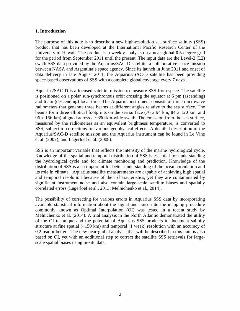
1. Introduction The purpose of this note is to describe a new high-resolution sea surface salinity (SSS) product that has been developed at the International Pacific Research Center of the University of Hawaii. The product is a weekly analysis on a near-global 0.5-degree grid for the period from September 2011 until the present. The input data are the Level-2 (L2) swath SSS data provided by the Aquarius/SAC-D satellite, a collaborative space mission between NASA and Argentina’s space agency. Since its launch in June 2011 and onset of data delivery in late August 2011, the Aquarius/SAC-D satellite has been providing space-based observations of SSS with a complete global coverage every 7 days.

Aquarius/SAC-D is a focused satellite mission to measure SSS from space. The satellite is positioned on a polar sun-synchronous orbit crossing the equator at 6 pm (ascending) and 6 am (descending) local time. The Aquarius instrument consists of three microwave radiometers that generate three beams at different angles relative to the sea surface. The beams form three elliptical footprints on the sea surface (76 x 94 km, 84 x 120 km, and 96 x 156 km) aligned across a ~390-km-wide swath. The emission from the sea surface, measured by the radiometers as an equivalent brightness temperature, is converted to SSS, subject to corrections for various geophysical effects. A detailed description of the Aquarius/SAC-D satellite mission and the Aquarius instrument can be found in Le Vine et al. (2007); and Lagerloef et al. (2008).

SSS is an important variable that reflects the intensity of the marine hydrological cycle. Knowledge of the spatial and temporal distribution of SSS is essential for understanding the hydrological cycle and for climate monitoring and prediction. Knowledge of the distribution of SSS is also important for better understanding of the ocean circulation and its role in climate. Aquarius satellite measurements are capable of achieving high spatial and temporal resolution because of their characteristics, yet they are contaminated by significant instrument noise and also contain large-scale satellite biases and spatially correlated errors (Lagerloef et al., 2013; Melnichenko et al., 2014).

The possibility of correcting for various errors in Aquarius SSS data by incorporating available statistical information about the signal and noise into the mapping procedure commonly known as Optimal Interpolation (OI) was tested in a recent study by Melnichenko et al. (2014). A trial analysis in the North Atlantic demonstrated the utility of the OI technique and the potential of Aquarius SSS products to document salinity structure at fine spatial (~150 km) and temporal (1 week) resolution with an accuracy of 0.2 psu or better. The new near-global analysis that will be described in this note is also based on OI, yet with an additional step to correct the satellite SSS retrievals for large-scale spatial biases using in-situ data.

3

2. Satellite SSS data, data quality control and correction for satellite biases

2.1. Aquarius SSS data

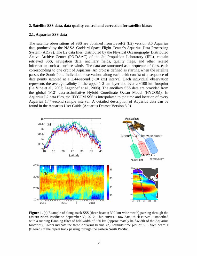
The satellite observations of SSS are obtained from Level-2 (L2) version 3.0 Aquarius data produced by the NASA Goddard Space Flight Center’s Aquarius Data Processing System (ADPS). The L2 data files, distributed by the Physical Oceanography Distributed Active Archive Center (PO.DAAC) of the Jet Propulsion Laboratory (JPL), contain retrieved SSS, navigation data, ancillary fields, quality flags, and other related information such as surface winds. The data are structured as a sequence of files, each corresponding to one orbit of Aquarius. An orbit is defined as starting when the satellite passes the South Pole. Individual observations along each orbit consist of a sequence of data points sampled at a 1.44-second (~10 km) interval. Each individual observation represents the average salinity in the upper 1-2 cm layer and over a ~100 km footprint (Le Vine et al., 2007; Lagerloef et al., 2008). The ancillary SSS data are provided from the global 1/12o data-assimilative Hybrid Coordinate Ocean Model (HYCOM). In Aquarius L2 data files, the HYCOM SSS is interpolated to the time and location of every Aquarius 1.44-second sample interval. A detailed description of Aquarius data can be found in the Aquarius User Guide (Aquarius Dataset Version 3.0).

Figure 1. (a) Example of along-track SSS (three beams; 390-km-wide swath) passing through the eastern North Pacific on September 30, 2012. Thin curves – raw data; thick curves – smoothed with a running Hanning filter of half-width of ~60 km (approximately half-width of the Aquarius footprint). Colors indicate the three Aquarius beams. (b) Latitude-time plot of SSS from beam 1 (filtered) of the repeat track passing through the eastern North Pacific.

10 15 20 25 30 35 4033

33.5

34

34.5

35

35.5

36

−160 −140 −120 −100 −80−60

−40

−20

0

20

40

60

(a)

10°N

20°N

30°N

40°N

S O N D J F M A M J J A S O N D J F M A M J J A S O N D

2012 20132011

33

34

35

36

(b)

96x156 km

Aquarius

3 beams, 390 km wide swath

76x94 km 84x120 km Latitude

4

An example of L2 SSS data is shown in Figure 1, illustrating that there are at least two types of errors in the SSS retrievals. A significant source of error is the accuracy of individual measurements along the satellite tracks. An important aspect of this error is its random character and a very short wavelength. This short-wavelength noise is essentially ‘white’ in nature and can effectively be suppressed by, for example, filtering the data along track such as shown in Figure 1 (heavy lines). Of much greater concern are differences between the three beams, which can be as large as 0.5-0.8 psu and appear to be correlated over large distances along the satellite tracks. This type of error is also illustrated by Figure 1. During the satellite pass over the eastern North Pacific on April 21, 2012, the middle beam (red) delivered systematically lower SSS as compared to the other two beams. Such inter-beam biases are likely a manifestation of residual geophysical corrections. Because the three radiometer beams view the ocean surface at slightly different angles, each beam is affected by geophysical errors differently (Lagerloef et al., 2013).

2.2. Data quality control

In order to produce the gridded product, the L2 SSS data are first checked for quality. All observations are discarded if they fail any of the following quality flags: 7 (direct solar flux contamination), 8 (reflected solar flux contamination), 9 (sun glint), 12 (non-nominal navigation), 13 (radiometer telemetry), 14 (roughness correction failure), 16 (pointing anomaly), 17 (brightness temperature consistency), 19 (radio-frequency interference (RFI)), and 21 (reflected radiation from Moon or Galaxy). In the case of flags 19 and 21, the data are excluded from the analysis if the conditions indicated by the flags are either moderate or severe. For other flags, only severe conditions are taken into account. Also excluded from the analysis are data points that are contaminated by land (land fraction > 0.005), sea ice (sea ice fraction > 0.005), sampled during high wind (wind speed > 15 m/s) and/or in cold water (SST < 5oC). A detailed description of the Aquarius quality flags including recommended thresholds can be found in the Aquarius User Guide (Aquarius Dataset Version 3.0).

2.3. Bias correction

The next step in data processing consists of a large-scale adjustment of the satellite data relative to in-situ data. Analysis of long time series of Aquarius SSS data revealed that satellite retrievals have large-scale biases relative to in-situ data (Hacker et al. 2014). Their spatial distribution show clear zonality with large negative biases (up to 0.4 psu) in the tropics and positive biases in mid- and high-latitudes (Hacker et al., 2014; Meissner et al., 2014). The causes of the biases in Aquarius data are only partially understood, but may be related to SST-dependent errors in the dielectric constant and the model for atmospheric absorption, which are part of the retrieval algorithm (Meissner et al., 2014).

5

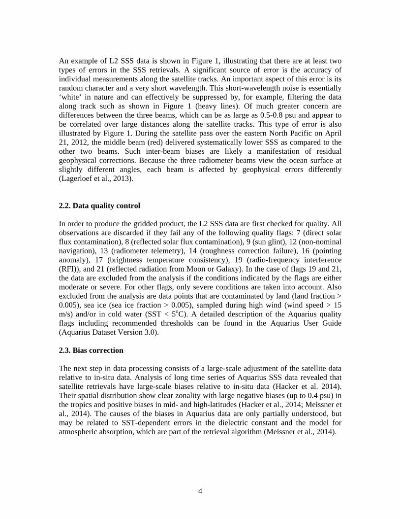
Figure 2. Mean spatial bias correction fields (psu) for Aquarius ascending (left) and descending (right) data; beam 1 (top), beam 2 (center), and beam 3 (bottom). Although the recent version of Aquarius data (3.0) includes an SST-adjusted SSS, the OI analysis described in this note utilizes standard SSS retrievals and implements an independent bias-correction algorithm. The SST-adjusted SSS, provided by the ADPS, is not utilized for the following reasons. First, the correction for the SST-dependent bias (in the form of quadratic regression on SST) has been developed using HYCOM SSS as a reference (Meissner et al., 2014) and thus can be subject to the model biases and uncertainties, arising from misrepresented physics, large gaps in the in-situ data coverage (in the case of data assimilation), errors in boundary conditions, etc. Second, the correction model uses ancillary SST fields, which are based on satellite SST observations optimally interpolated on a regular grid and which, in turn, include some sort of bias adjustment (Reynolds et al., 2007). In addition, SST fields exhibit patterns of strong seasonal cycle, which are not the same for SSS due to different natures of the forcing. As a result, the SST-dependent adjustment may introduce some false signals to the seasonal cycle in SSS. Finally, there are strong SST fronts, particularly in the tropics and along strong boundary currents, which are not necessarily associated with SSS fronts. In such

0 60 120 180 240 300 0 60

−60

−40

−20

0

20

40

60

0 60 120 180 240 300 0 60

−60

−40

−20

0

20

40

60

0 60 120 180 240 300 0 60

−60

−40

−20

0

20

40

60

(a)

(b)

(c)

0 60 120 180 240 300 0 60

−60

−40

−20

0

20

40

60

−0.2

−0.1

0

0.1

0.2

0 60 120 180 240 300 0 60

−60

−40

−20

0

20

40

60

−0.2

−0.1

0

0.1

0.2

0 60 120 180 240 300 0 60

−60

−40

−20

0

20

40

60

−0.2

−0.1

0

0.1

0.2

(d)

(e)

(f)

6

cases, the SST-dependent adjustment may cause appearance of false SSS fronts or distort the true signal.

In the OI analysis, satellite biases are corrected relative to in-situ salinity data collected by Argo floats. The bias fields were constructed by differencing the Argo- and Aquarius-derived SSS fields. The latter were derived using only ascending or only descending satellite observations and also separately for each of the three Aquarius beans. For this purpose, because of the large spatial structure of the biases (Hacker et al., 2014), the large-scale SSS fields from Aquarius were constructed by bin-averaging of raw Aquarius observations within 4ox4o spatial bins centered on a global grid with the grid spacing of 2o in both longitude and latitude directions. The Argo-derived fields, which we regard as the “ground truth” at large spatial scales, are monthly-mean SSS fields obtained with variational interpolation of Argo buoy measurements (APDRC product). Only systematic, time-averaged biases are taken into account. Thus, there are six bias fields, shown in Figure 2. In order to remove the unwanted small-scale signals, arising primarily from irregular sampling, the bias fields were smoothed with a two-dimensional running Hanning window of half-width of 10o, generally consistent with the smoothness properties of the Argo-derived salinity fields.

The bias-adjusted satellite observations adjS are determined from the retrieved values

obsS as SSS obsadj Δ−= , (1)

where the bias SΔ is determined by interpolating the bias fields, shown in Figure 2, into the locations of the satellite measurements according to the corresponding Aquarius beam and ascending/descending mode. 3.4. Filtering

The final step in data preparation consists of filtering the data along track as described in Melnichenko et al. (2014). The filter is a low pass Hanning filter of half-width of ~60 km (six times the along-track sampling), which has been found to perform quite efficiently to considerably reduce high-frequency instrument noise, yet preserve the ocean signal from over-smoothing (Melnichenko et al., 2014). An example is presented in Figure 1a. According to the degree of filtering, the SSS data are then sub-sampled every third point along track.

3. General description of OI algorithm

The interpolation expression for OI with N observations can be written as (Bretherton et al., 1976; Le Traon et al., 1998):

∑∑= =

− −+=N

i

N

ji

obsixjijxx SSCASS

1 1

010 )(ˆ , (2)

7

where xS is the interpolated value (or estimate) at the grid point x ; 0xS is the forecast

(or “first guess”) value at the grid point x ; obsiS is the measured value at the observation

point i : iiobsi SS ε+= , where iε is random measurement error; 0

iS is the forecast value at the observation point i ; A is the NN × covariance matrix of the data ><+>−−=< jijjiiij SSSSA εε))(( 00 ; (3) and C is the joint covariance of the data and the field to be estimated >−−=< ))(( 00

jjxxxj SSSSC . (4) In (3) and (4), it is assumed (as is usually reasonable) that the errors and the field are not correlated. Analysis of Aquarius along track SSS data (e.g., Figure 1) reveals that there are long-wavelength errors, referred to here as inter-beam biases, which are correlated over long distances along the satellite tracks. To incorporate statistical information on these errors into the OI scheme, we adopt the idea that has originally been developed for altimeter applications (e.g., Le Traon et al. 1998) and introduce the error covariance model for the Aquarius data in the form

22Lwijji σσδεε +>=< -if data points ji, are on the same track and

beam, and in the same cycle, and 2

wijji σδεε >=< -otherwise,

where ijδ is the Kronecker delta, 2wσ is the variance of the uncorrelated (white) noise,

and 2Lσ is the variance of the long-wavelength (along-track) error.

Thus, the algorithm allows two types of random errors to contribute to the elements of the error covariance matrix: the white noise (diagonal elements), representing uncorrelated errors, and the long-wavelength error (off-diagonal elements), representing inter-beam biases that correlate over long distances along the satellite tracks. Each Aquarius beam is modeled as having independent errors.

The OI analysis is determined relative to the first guess field, which is assumed to be a good approximation of the true state. The estimate and the observations are then equal to the first guess plus small increments. In this way, the grid point analysis consists of interpolation of the first-guess field to the observation points followed by interpolation of the differences between the observed and first-guess values back to the grid point. The grid point analysis is completed by adding the analysis increment to the first guess.

8

4. Specifics

The OI method assumes that the first guess and statistics of the field to be analyzed are known a priory. These parameters are the following.

4.1. First guess

The first guess fields are derived from monthly-mean SSS fields produced by the APDRC with variational interpolation of Argo buoy measurements. An example for the first week of September 2011 is presented in Figure 3a. The Argo-derived SSS fields are chosen because they are independent of the analysis of the satellite data and provide unbiased estimates of the first guess as compared to, say, climatological fields, which can be biased at large-scales due to the presence of significant trends related to climate change or due to their reliance on highly inhomogeneous multi-type-instrument historical data.

4.2. Signal statistics

The normalized spatial covariance of weekly SSS anomalies is described by the Gaussian function of the form )//exp(),( 2222

yyxxyx RrRrrrC −−= , (5)

where xr and yr are spatial lags in the zonal and meridional directions, respectively, and

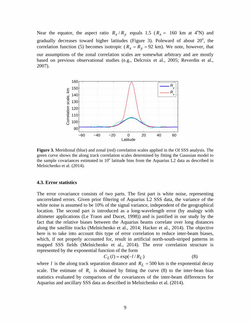
xR and yR are the zonal and meridional correlation scales. This particular form of the correlation structure is chosen because the associated spectrum is positive everywhere and because the resulting covariance matrixes are always positive definite (Weber and Talkner, 1993), which is a strict requirement on the choice of a possible analytical form of the correlation function in the OI analysis (Gandin, 1965; Bretherton et al., 1976). Both the zonal and meridional correlation scales in Eq. (5) are allowed to vary with latitude. The meridional scales have been determined by fitting the Gaussian model to the sample covariances estimated in 10o latitude bins from the Aquarius L2 data as described in Melnichenko et al. (2014). Based on the observed structure (Figure 3), the latitudinal dependency of yR is modeled by the following functional form

92))225/)4(exp(14)( 2 +−−= yyRy km, (6) where y is latitude in degrees. Thus, the meridional scales are somewhat larger in the tropics (106 km at 4oN) than at high latitudes (92 km). The zonal correlation scales at mid- and high latitudes are set to equal the meridional scales, while in the tropics they are scaled to represent the zonal elongation of correlation as follows )1)25.56/)4(exp(5.0)(()( 2 +−−= yyRyR yx . (7)

9

−60 −40 −20 0 20 40 60

90

100

110

120

130

140

150

160

Latitude

Cor

rela

tion

scal

e, k

m

R

y

Rx

Near the equator, the aspect ratio yx RR / equals 1.5 ( =xR 160 km at 4oN) and gradually decreases toward higher latitudes (Figure 3). Poleward of about 20o, the correlation function (5) becomes isotropic ( == yx RR 92 km). We note, however, that our assumptions of the zonal correlation scales are somewhat arbitrary and are mostly based on previous observational studies (e.g., Delcroix et al., 2005; Reverdin et al., 2007). Figure 3. Meridional (blue) and zonal (red) correlation scales applied in the OI SSS analysis. The green curve shows the along track correlation scales determined by fitting the Gaussian model to the sample covariances estimated in 10o latitude bins from the Aquarius L2 data as described in Melnichenko et al. (2014). 4.3. Error statistics

The error covariance consists of two parts. The first part is white noise, representing uncorrelated errors. Given prior filtering of Aquarius L2 SSS data, the variance of the white noise is assumed to be 10% of the signal variance, independent of the geographical location. The second part is introduced as a long-wavelength error (by analogy with altimeter applications (Le Traon and Ducet, 1998)) and is justified in our study by the fact that the relative biases between the Aquarius beams correlate over long distances along the satellite tracks (Melnichenko et al., 2014; Hacker et al., 2014). The objective here is to take into account this type of error correlation to reduce inter-beam biases, which, if not properly accounted for, result in artificial north-south-striped patterns in mapped SSS fields (Melnichenko et al., 2014). The error correlation structure is represented by the exponential function of the form

)/exp()( LL RllC −= (8) where l is the along track separation distance and =LR 500 km is the exponential decay scale. The estimate of LR is obtained by fitting the curve (8) to the inter-bean bias statistics evaluated by comparison of the covariances of the inter-beam differences for Aquarius and ancillary SSS data as described in Melnichenko et al. (2014).

10

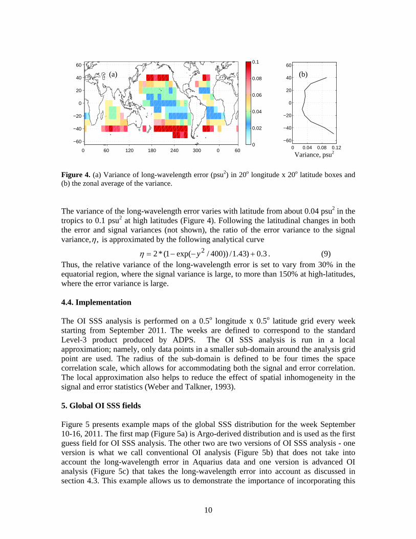
Figure 4. (a) Variance of long-wavelength error (psu2) in 20o longitude x 20o latitude boxes and (b) the zonal average of the variance. The variance of the long-wavelength error varies with latitude from about 0.04 psu2 in the tropics to 0.1 psu2 at high latitudes (Figure 4). Following the latitudinal changes in both the error and signal variances (not shown), the ratio of the error variance to the signal variance, ,η is approximated by the following analytical curve

3.0)43.1/))400/exp(1(*2 2 +−−= yη . (9) Thus, the relative variance of the long-wavelength error is set to vary from 30% in the equatorial region, where the signal variance is large, to more than 150% at high-latitudes, where the error variance is large. 4.4. Implementation

The OI SSS analysis is performed on a 0.5o longitude x 0.5o latitude grid every week starting from September 2011. The weeks are defined to correspond to the standard Level-3 product produced by ADPS. The OI SSS analysis is run in a local approximation; namely, only data points in a smaller sub-domain around the analysis grid point are used. The radius of the sub-domain is defined to be four times the space correlation scale, which allows for accommodating both the signal and error correlation. The local approximation also helps to reduce the effect of spatial inhomogeneity in the signal and error statistics (Weber and Talkner, 1993).

5. Global OI SSS fields

Figure 5 presents example maps of the global SSS distribution for the week September 10-16, 2011. The first map (Figure 5a) is Argo-derived distribution and is used as the first guess field for OI SSS analysis. The other two are two versions of OI SSS analysis - one version is what we call conventional OI analysis (Figure 5b) that does not take into account the long-wavelength error in Aquarius data and one version is advanced OI analysis (Figure 5c) that takes the long-wavelength error into account as discussed in section 4.3. This example allows us to demonstrate the importance of incorporating this

0 60 120 180 240 300 0 60

−60

−40

−20

0

20

40

60

0

0.02

0.04

0.06

0.08

0.1

0 0.04 0.08 0.12

−60

−40

−20

0

20

40

60

(a) (b)

Variance, psu2

11

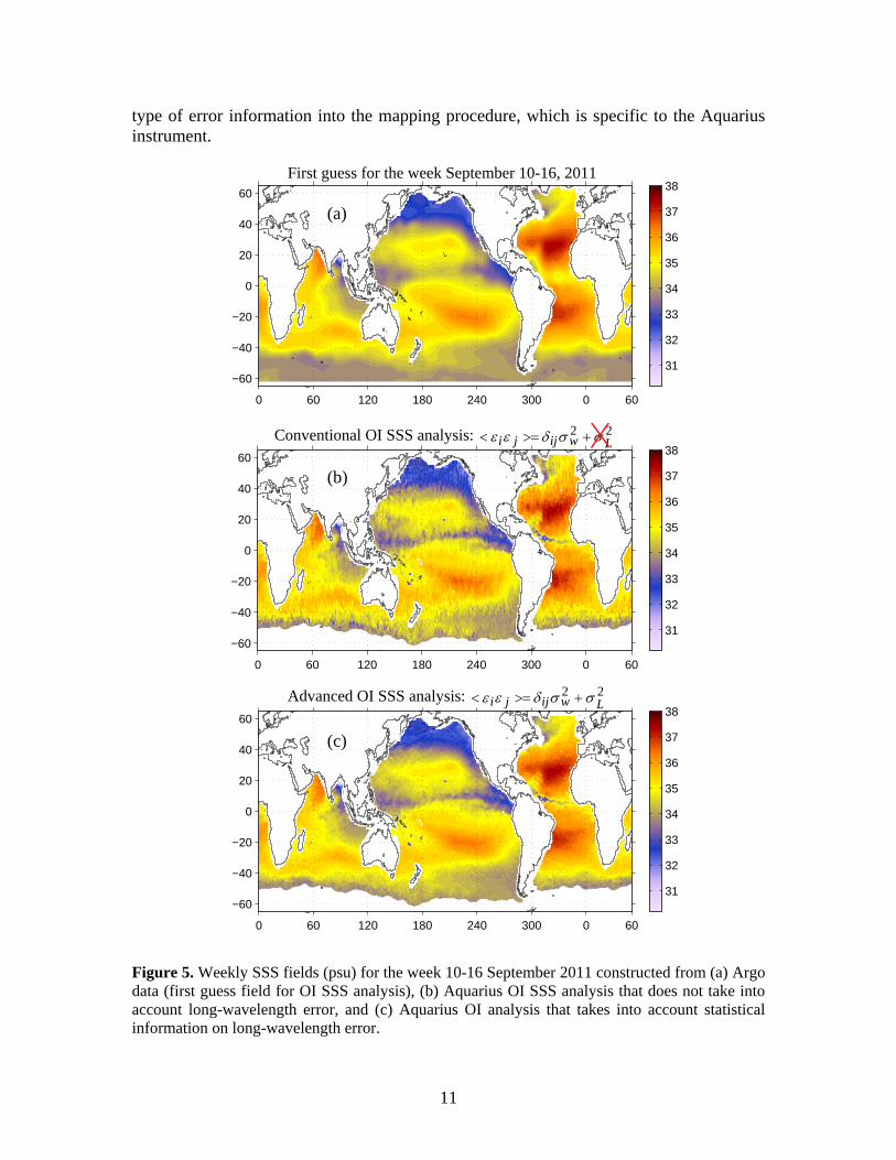
type of error information into the mapping procedure, which is specific to the Aquarius instrument. Figure 5. Weekly SSS fields (psu) for the week 10-16 September 2011 constructed from (a) Argo data (first guess field for OI SSS analysis), (b) Aquarius OI SSS analysis that does not take into account long-wavelength error, and (c) Aquarius OI analysis that takes into account statistical information on long-wavelength error.

0 60 120 180 240 300 0 60

−60

−40

−20

0

20

40

60

31

32

33

34

35

36

37

38Advanced OI SSS analysis: 22

Lwijji σσδεε +>=<

0 60 120 180 240 300 0 60

−60

−40

−20

0

20

40

60

31

32

33

34

35

36

37

38Conventional OI SSS analysis: 22

Lwijji σσδεε +>=<

0 60 120 180 240 300 0 60

−60

−40

−20

0

20

40

60

31

32

33

34

35

36

37

38First guess for the week September 10-16, 2011

(c)

(b)

(a)

12

0 60 120 180 240 300 0 60

−60

−40

−20

0

20

40

60

0.05

0.1

0.15

0.2

0.25

0.3

0.35

0.4

0.45

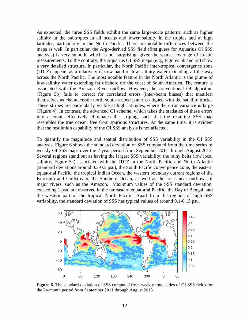
As expected, the three SSS fields exhibit the same large-scale patterns, such as higher salinity in the subtropics in all oceans and lower salinity in the tropics and at high latitudes, particularly in the North Pacific. There are notable differences between the maps as well. In particular, the Argo-derived SSS field (first guess for Aquarius OI SSS analysis) is very smooth, which is not surprising, given the sparse coverage of in-situ measurements. To the contrary, the Aquarius OI SSS maps (e.g., Figures 5b and 5c) show a very detailed structure. In particular, the North Pacific inter-tropical convergence zone (ITCZ) appears as a relatively narrow band of low-salinity water extending all the way across the North Pacific. The most notable feature in the North Atlantic is the plume of low-salinity water extending far offshore off the coast of South America. The feature is associated with the Amazon River outflow. However, the conventional OI algorithm (Figure 5b) fails to correct for correlated errors (inter-beam biases) that manifest themselves as characteristic north-south-striped patterns aligned with the satellite tracks. These stripes are particularly visible at high latitudes, where the error variance is large (Figure 4). In contrast, the advanced OI scheme, which takes the statistics of these errors into account, effectively eliminates the striping, such that the resulting SSS map resembles the true ocean, free from spurious structures. At the same time, it is evident that the resolution capability of the OI SSS analysis is not affected. To quantify the magnitude and spatial distribution of SSS variability in the OI SSS analysis, Figure 6 shows the standard deviation of SSS computed from the time series of weekly OI SSS maps over the 2-year period from September 2011 through August 2013. Several regions stand out as having the largest SSS variability: the rainy belts (low local salinity, Figure 5c) associated with the ITCZ in the North Pacific and North Atlantic (standard deviations around 0.3-0.5 psu), the South Pacific convergence zone, the eastern equatorial Pacific, the tropical Indian Ocean, the western boundary current regions of the Kuroshio and Gulfstream, the Southern Ocean, as well as the areas near outflows of major rivers, such as the Amazon. Maximum values of the SSS standard deviation, exceeding 1 psu, are observed in the far eastern equatorial Pacific, the Bay of Bengal, and the western part of the tropical North Pacific. Apart from the regions of high SSS variability, the standard deviation of SSS has typical values of around 0.1-0.15 psu. Figure 6. The standard deviation of SSS computed from weekly time series of OI SSS fields for the 24-month period from September 2011 through August 2013.

13

−0.04

−0.02

0

0.02

0.04

Mea

n D

iffer

ence

, psu

(a)

0.1

0.15

0.2

0.25

0.3

RM

SD

, psu

S O N D J F M A M J J A S O N D J F M A M J J A S O N D J F M2011 2012 2013

(b)

6. Validation

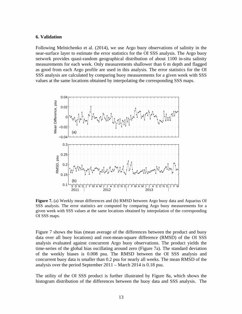
Following Melnichenko et al. (2014), we use Argo buoy observations of salinity in the near-surface layer to estimate the error statistics for the OI SSS analysis. The Argo buoy network provides quasi-random geographical distribution of about 1100 in-situ salinity measurements for each week. Only measurements shallower than 6 m depth and flagged as good from each Argo profile are used in this analysis. The error statistics for the OI SSS analysis are calculated by comparing buoy measurements for a given week with SSS values at the same locations obtained by interpolating the corresponding SSS maps. Figure 7. (a) Weekly mean differences and (b) RMSD between Argo buoy data and Aquarius OI SSS analysis. The error statistics are computed by comparing Argo buoy measurements for a given week with SSS values at the same locations obtained by interpolation of the corresponding OI SSS maps. Figure 7 shows the bias (mean average of the differences between the product and buoy data over all buoy locations) and root-mean-square difference (RMSD) of the OI SSS analysis evaluated against concurrent Argo buoy observations. The product yields the time-series of the global bias oscillating around zero (Figure 7a). The standard deviation of the weekly biases is 0.008 psu. The RMSD between the OI SSS analysis and concurrent buoy data is smaller than 0.2 psu for nearly all weeks. The mean RMSD of the analysis over the period September 2011 – March 2014 is 0.18 psu. The utility of the OI SSS product is further illustrated by Figure 8a, which shows the histogram distribution of the differences between the buoy data and SSS analysis. The

14

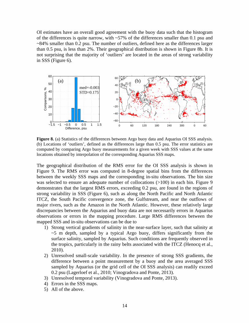
OI estimates have an overall good agreement with the buoy data such that the histogram of the differences is quite narrow, with ~57% of the differences smaller than 0.1 psu and ~84% smaller than 0.2 psu. The number of outliers, defined here as the differences larger than 0.5 psu, is less than 2%. Their geographical distribution is shown in Figure 8b. It is not surprising that the majority of ‘outliers’ are located in the areas of strong variability in SSS (Figure 6).

Figure 8. (a) Statistics of the differences between Argo buoy data and Aquarius OI SSS analysis. (b) Locations of ‘outliers’, defined as the differences large than 0.5 psu. The error statistics are computed by comparing Argo buoy measurements for a given week with SSS values at the same locations obtained by interpolation of the corresponding Aquarius SSS maps.

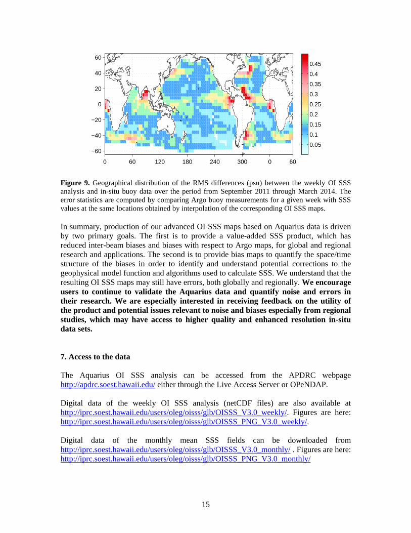
The geographical distribution of the RMS error for the OI SSS analysis is shown in Figure 9. The RMS error was computed in 8-degree spatial bins from the differences between the weekly SSS maps and the corresponding in-situ observations. The bin size was selected to ensure an adequate number of collocations (>100) in each bin. Figure 9 demonstrates that the largest RMS errors, exceeding 0.2 psu, are found in the regions of strong variability in SSS (Figure 6), such as along the North Pacific and North Atlantic ITCZ, the South Pacific convergence zone, the Gulfstream, and near the outflows of major rivers, such as the Amazon in the North Atlantic. However, these relatively large discrepancies between the Aquarius and buoy data are not necessarily errors in Aquarius observations or errors in the mapping procedure. Large RMS differences between the mapped SSS and in-situ observations can be due to

1) Strong vertical gradients of salinity in the near-surface layer, such that salinity at ~5 m depth, sampled by a typical Argo buoy, differs significantly from the surface salinity, sampled by Aquarius. Such conditions are frequently observed in the tropics, particularly in the rainy belts associated with the ITCZ (Henocq et al., 2010).

2) Unresolved small-scale variability. In the presence of strong SSS gradients, the difference between a point measurement by a buoy and the area averaged SSS sampled by Aquarius (or the grid cell of the OI SSS analysis) can readily exceed 0.2 psu (Lagerloef et al., 2010; Vinogradova and Ponte, 2013).

3) Unresolved temporal variability (Vinogradova and Ponte, 2013). 4) Errors in the SSS maps. 5) All of the above.

−1.5 −1 −0.5 0 0.5 1 1.50

10

20

30

40

50

60

Difference, psu

Com

paris

ons,

%

0 60 120 180 240 300 0 60

−60

−40

−20

0

20

40

60(a) (b)

med=-0.003 STD=0.175

15

0 60 120 180 240 300 0 60

−60

−40

−20

0

20

40

60

0.05

0.1

0.15

0.2

0.25

0.3

0.35

0.4

0.45

Figure 9. Geographical distribution of the RMS differences (psu) between the weekly OI SSS analysis and in-situ buoy data over the period from September 2011 through March 2014. The error statistics are computed by comparing Argo buoy measurements for a given week with SSS values at the same locations obtained by interpolation of the corresponding OI SSS maps. In summary, production of our advanced OI SSS maps based on Aquarius data is driven by two primary goals. The first is to provide a value-added SSS product, which has reduced inter-beam biases and biases with respect to Argo maps, for global and regional research and applications. The second is to provide bias maps to quantify the space/time structure of the biases in order to identify and understand potential corrections to the geophysical model function and algorithms used to calculate SSS. We understand that the resulting OI SSS maps may still have errors, both globally and regionally. We encourage users to continue to validate the Aquarius data and quantify noise and errors in their research. We are especially interested in receiving feedback on the utility of the product and potential issues relevant to noise and biases especially from regional studies, which may have access to higher quality and enhanced resolution in-situ data sets. 7. Access to the data The Aquarius OI SSS analysis can be accessed from the APDRC webpage http://apdrc.soest.hawaii.edu/ either through the Live Access Server or OPeNDAP. Digital data of the weekly OI SSS analysis (netCDF files) are also available at http://iprc.soest.hawaii.edu/users/oleg/oisss/glb/OISSS_V3.0_weekly/. Figures are here: http://iprc.soest.hawaii.edu/users/oleg/oisss/glb/OISSS_PNG_V3.0_weekly/. Digital data of the monthly mean SSS fields can be downloaded from http://iprc.soest.hawaii.edu/users/oleg/oisss/glb/OISSS_V3.0_monthly/ . Figures are here: http://iprc.soest.hawaii.edu/users/oleg/oisss/glb/OISSS_PNG_V3.0_monthly/

16

8. Copyright and terms of use The Aquarius OI SSS dataset is open for free unrestricted use. The dataset is a research quality product. Errors reported to the authors by users will be published and corrected in the next update of the dataset. Use of the dataset should be acknowledged as follows: “This study used Aquarius sea surface salinity optimal interpolation analysis provided by APDRC/IPRC of the University of Hawaii”. Reference to this technical paper: Melnichenko, O., P. Hacker, N. Maximenko, G. Lagerloef, and J. Potemra: Aquarius sea surface salinity optimal interpolation analysis, IPRC Technical Note No. 6, October 7, 2014, 18p. Comments, questions regarding the Aquarius OI SSS dataset and requests for the data can be directed to any of the authors: Oleg Melnichenko Email: oleg@hawaii.edu Tel: 1-808-956-0747 Peter Hacker Email: phacker@hawaii.edu Nikolai Maximenko Email: maximenk@hawaii.edu Gary Lagerloef Earth and Space Research Email: lager@esr.org James Potemra Email: jimp@hawaii.edu

9. Acknowledgements This project was supported by the National Aeronautic and Space Administration (NASA) Ocean Salinity Science Team through grant NNX12AK52G and grant NNX12AK52G. Additional support was provided by the Japan Agency for Marine-Earth Science and Technology (JAMSTEC), by NASA through grant NNX07AG53G, and by National Oceanic and Atmospheric Administration through grant NA17RJ1230 through their sponsorship of research activities at the International Pacific Research Center (IPRC). The Argo data were collected and made freely available by the International Argo Program and the national programs that contribute to it (http://www.argo.ucsd.edu).

17

The Argo Program is part of the Global Ocean Observing System. The authors acknowledge the many constructive dialogues with the members of the Aquarius calibration/validation team.

10. References Aquarius User Guide (Aquarius Dataset Version 3.0), 2 June 2014, Document AQ-010-

UG-0008, available at: ftp://podaac-ftp.jpl.nasa.gov/allData/aquarius/docs/v3/AQ-010-UG-0008_AquariusUserGuide_DatasetV3.0.pdf

Bretherton, F. P., R.E Davis, and C.B. Fandry, 1976: A technique for objective analysis

and design of oceanographic experiments applied to MODE-73, Deep Sea Res., 23, 559-582.

Delcroix, T., M.J. McPhaden, A. Dessier, and Y. Gouriou, 2005: Time and space scales

for sea surface salinity in the tropical ocean, Deep-Sea Res. I, 52, 787-813. Gandin, L.S., 1965: Objective Analysis of Meteorological Fields, 242 pp, Israel Program

for Scientific Translation, Jerusalem. Hacker, P., O. Melnichenko, N. Maximenko, and J. Potemra, 2014: Aquarius Sea Surface

Salinity Observations for Global and Regional Studies: Error Analysis and Applications, 2014 Ocean Sciences Meeting, February 23-28, 2014, Honolulu, Hawaii; e-poster, available at: http://www.eposters.net/pdfs/aquarius-sea-surface-salinity-observations-for-global-and-regional-studies-error-analysis-and.pdf.

Henocq, C., J. Boutin, F. Petitcolin, G. Reverdin, S. Arnault, and P. Lattes, 2010: Vertical

variability of Near-Surface Salinity in the Tropics: Consequences for L-Band Radiometer Calibration and Validation, J. Atmos. Oceanic Technol., 27, 192-209.

Lagerloef, G., F.R. Colomb, D. LeVine, F. Wentz, S. Yueh, C. Ruf, J. Lilly, J. Gunn, Y.

Chao, A. deCharon, G. Feldman, and C. Swift, 2008: The Aquarius/SAC-D Mission: Designed to meet the salinity remote-sensing challenge, Oceanography, 20, 68-81.

Lagerloef, G., H.-Y. Kao, O. Melnichenko, P. Hacker, Eric Hackert, Y. Chao, K. Hilburn,

T. Meissner, S. Yueh, L. Hong, and T. Lee, 2013: Aquarius salinity Validation Analysis, Aquarius project document AQ-014-PS-0016, JPL, 18 February 2013, available at ftp://podaac-ftp.jpl.nasa.gov/allData/aquarius/docs/v2/AQ-014-PS-0016_AquariusSalinityDataValidationAnalysis_DatasetVersion2.0.pdf.

Lagerloef, G., J. Boutin, Y. Chao, T. Delcroix, J. Font, P. Niiler, N. Reul, S. Riser, R.

Schmitt, D. Stammer, and F. Wentz, 2010: Resolving the global surface salinity field and variability by blending satellite and in situ observations, In Proceedings of

18

OceanObs’09: Sustained Ocean Observations and Information for Society (Vol. 2), Venice, Italy, 21-25 September 2009, Hall, J., Harrison, D.E. & Stammer, D. Eds., ESA Publication WPP-306, doi:105270/OceanObs09.cwp.51.

Le Traon, P.Y., F. Nadal, and N. Ducet, 1998: An improved mapping method of

multisatellite altimeter data, J. Atmos. Oceanic Technol., 15, 522-534. Le Vine, D.M., G.S.E. Lagerloef, F.R. Colomb, S.H. Yueh, and F.A. Pellerano, 2007:

Aquarius: An instrument to monitor sea surface salinity from Space, IEEE Transactions on Geoscience and Remote Sensing, 45, 2040-2050.

Meissner, T., F. Wentz, D. LeVine, and J. Scott, 2014: Addendum III to ATBD, 4 June

2011, available at: ftp://podaac-ftp.jpl.nasa.gov/allData/aquarius/docs/v3/AQ-014-PS-0017_AquariusATBD_Level2_Addendum3_DatasetVersion3.0.pdf

Melnichenko, O., P. Hacker, N. Maximenko, G. Lagerloef, and J. Potemra, 2014: Spatial

Optimal Interpolation of Aquarius Sea Surface Salinity: Algorithms and Implementation in the North Atlantic, J. Atmos. Oceanic Technol., 31, 1583-1600.

Reynolds, R.W., T.M. Smith, C. Liu, D.B. Chelton, K.S. Casey, and M. Schlax, 2007:

Daily High-Resolution-Blended Analyses for Sea Surface Temperature, J. Clim., 20, 5473-5496.

Reverdin, G., E. Kestenare, C. Frankignoul, and T. Delcroix, 2007: Surface salinity in the

Atlantic Ocean (30oS-50oN), Prog. Oceanogr., 73, 311-340. Vinogradova, N. T., and R.M. Ponte, 2013: Small-scale variability in sea surface salinity

and implications for satellite-derived measurements, J. Atmos. Oceanic Technol., 30, 2689-2694.

Weber, R.O., and P. Talkner, 1993: Some Remarks on Spatial Correlation Function

Models, Mon. Wea. Rev., 121, 2611-2617.