AQWA: Adaptive Query­Workload­Aware Partitioning ofBig Spatial Data

Ahmed M. Aly1, Mohamed S. Hassan1, Ahmed R. Mahmood1, Walid G. Aref1,Hazem Elmeleegy2, Mourad Ouzzani3

1Purdue University, West Lafayette, IN2Turn Inc., Redwood City, CA

3Qatar Computing Research Institute, Doha, Qatar1{aaly, msaberab, aref, amahmoo}@cs.purdue.edu,2hazem.elmeleegy@turn.com, 3mouzzani@qf.org.qa

ABSTRACTThe unprecedented spread of location-aware devices has resultedinto a plethora of location-based services in which huge amountsof spatial data need to be efficiently processed. To process large-scale data, MapReduce has become the de facto framework forlarge-scale computing clusters. Existing cluster-based systems forprocessing spatial data are oblivious to query-workload, and henceare not able to consistently provide good performance. The reasonis that typical spatial query-workloads exhibit skewed access pat-terns, where certain spatial areas receive queries more frequentlythan others. To close this gap, we present AQWA, an adaptive andquery-workload-aware data partitioning mechanism that minimizesthe processing time of spatial queries over large-scale spatial data.AQWA does not assume prior knowledge of the query-workload.Instead, AQWA adapts to the query-workload, and in an onlinefashion. As queries get processed, the data partitions are incremen-tally updated. With extensive experiments using real spatial data ofBillions of points from OpenStreetMap, and thousands of spatialrange and k-nearest-neighbor queries executed over a cluster run-ning Hadoop, we demonstrate that AQWA can achieve orders ofmagnitude gain in query performance compared to standard spatialpartitioning structures.

1. INTRODUCTIONThe ubiquity of location-aware devices, e.g., smartphones and

GPS-devices, has led to a large variety of location-based servicesin which large amounts of geo-tagged information are created ev-ery day. Meanwhile, the MapReduce framework [10] has provento be very successful in processing large datasets on large clusters,particularly after the massive deployments reported by companieslike Facebook, Google, and Yahoo!. Moreover, tools built on top ofHadoop [34], the open-source implementation of Mapreduce, e.g.,Pig [25], Hive [31], Cheetah [6], and Pigeon [12], make it easier forusers to engage with Hadoop and run queries using high-level lan-guages. However, one of the main issues with MapReduce is that

Permission to make digital or hard copies of all or part of this work forpersonal or classroom use is granted without fee provided that copies arenot made or distributed for profit or commercial advantage and that copiesbear this notice and the full citation on the first page. To copy otherwise, torepublish, to post on servers or to redistribute to lists, requires prior specificpermission and/or a fee. Articles from this volume were invited to presenttheir results at The xth International Conference on Very Large Data Bases.Proceedings of the VLDB Endowment, Vol. X, No. YCopyright 20xy VLDB Endowment 2150­8097/11/XX... $ 10.00.

executing a query usually involves scanning very large amounts ofdata that can lead to high response times. Not enough attention hasbeen devoted to addressing this issue in the context of spatial data.

As noted in several research efforts, e.g., [26, 32, 8], account-ing for the query-workload can achieve significant performancegains. In particular, regions of space that are queried with highfrequency need to be aggressively partitioned in comparison to theother less popular regions. This fine-grained partitioning of thein-high-demand data can result in significant savings in query pro-cessing time.

Existing cluster-based systems for processing spatial data em-ploy traditional spatial indexing methods that can effectively parti-tion the data into multiple buckets, but that are not query-workloadaware. For instance, SpatialHadoop [11, 13] supports both space-partitioning as well as data-partitioning schemes to handle spatialdata on Hadoop. However, both partitioning schemes are static anddo not adapt to changes in query-workload.

In this paper, we present AQWA, an adaptive and query-workload aware data partitioning mechanism that minimizes thequery processing time of spatial queries over large-scale spatialdata. An important characteristic of AQWA is that it does not pre-sume any knowledge of the query-workload. Instead, AQWA candetect, in an online fashion, the pattern(s) of the query-workload,e.g., when certain spatial regions get queried more frequently thanother spatial regions. Accordingly, AQWA reorganizes the data ina way that better serves the execution of the queries by minimizingthe amount of data to be scanned. Furthermore, AQWA can adaptto changes in the query-workload. Instead of recreating the parti-tions from scratch, which is a costly operation because it requiresreading and writing the entire data, AQWA incrementally updatesthe partitioning of the data in an online fashion.

Observe that the number of ways one can partition the underlyingspatial data is large. Finding the boundaries of the partitions thatwould result in good performance gains for a given query-workloadis challenging. The process of searching for the optimal partition-ing involves excessive use of two operations: 1) Finding the num-ber of points in a given region, and 2) Finding the number of queriesthat overlap a given region. A straightforward way to support thesetwo operations is to scan the whole data (in case of Operation 1)and all queries in the workload (in case of Operation 2), which isquite costly. The reason is that: i) we are dealing with big data inwhich scanning the whole data is costly, and ii) the two operationsare to be repeated multiple times in order to find the best partition-ing. To address this challenge, AQWA employes various optimiza-tions to support the above two operations efficiently. In particular,AQWA maintains a set of compact aggregate information about the

data distribution as well as the query-workload. This aggregate in-formation is kept in main-memory, and hence it enables AQWA toefficiently perform its adaptive repartitioning decisions.

Unlike traditional spatial index structures that can have un-bounded decomposition until the finest granularity of data isreached in each split (i.e., block), AQWA tries to limit the num-ber of partitions (i.e., files) because allowing too many small par-titions can be very harmful to the overall health of a computingcluster. The metadata of the partitions is usually managed in a cen-tralized shared resource. For instance, the name node is a central-ized resource in Hadoop that manages the metadata of the files inthe Hadoop Distributed File System (HDFS), and handles the filerequests across the whole cluster. Hence, the name node is a criti-cal component in Hadoop, and if overloaded with too many (small)files, it slows down the overall cluster (e.g., see [2, 18, 22, 33,35]). Being of vital importance to a Hadoop cluster, the latest re-leases of Hadoop try to maintain more than one replica of the namenode in order to increase the cluster availability in case of failures.However, replication of the name node does not help distribute theoverhead of maintaining the data partitions, and hence in AQWA,we limit the number of data partitions in order to overcome thischallenge.

AQWA employs a simple yet powerful cost function that modelsthe cost of executing the queries and also associates with each datapartition the corresponding cost. To incrementally update the datapartitions and maintain a limited number of partitions, AQWA se-lects some partition(s) to be split (if queried with high frequency)and other partition(s) to be merged (if queried with low frequency).To efficiently select the best data partitions to split and merge,AQWA maintains dual priority queues in main-memory; one pri-ority queue stores the cost gain corresponding to splitting a datapartition (a max-heap), and the other priority queue stores the costloss corresponding to merging data partitions (a min-heap).

AQWA is resilient to abrupt or temporary changes in the work-load. Based on the cost model, an invariant relationship guards theoperation of the dual priority queues to make sure that no redundantsplit/merge operations take place. However, when the workloadpermanently shifts from one hotspot area (i.e., one that receivesqueries more frequently, e.g., downtown area) to another hotspotarea, AQWA is able to react to that change and update the partition-ing accordingly. To achieve that, AQWA employs a time-fadingcounting mechanism that alleviates the weights corresponding toolder query-workloads.

In summary, the contributions of the paper are as follows.

• We introduce AQWA, a new dynamic data partitioningscheme that is query-workload-aware. AQWA is able to:1) partition the data without prior knowledge of the query-workload, 2) incrementally update the partitions (accordingto the workload) rather than rebuilding the partitions fromscratch, and 3) automatically adapt to changes in the work-load, e.g., when the workload shifts over time from one spa-tial hotspot to another hotspot.

• We present efficient algorithms for supporting two basic op-erations that are at the core of AQWA’s partitioning mecha-nism, namely finding the number of points in a given region,and finding the number of queries in a workload that overlapa given region.

• We adopt a cost-based dual priority queue mechanism thatmanages the process of repartitioning the data by taking intoconsideration the cost saving/loss associated with each pos-sible split/merge of a data partition.

• We evaluate the performance of AQWA on a Hadoop clusterby executing various query-workloads of spatial range andk-nearest-neighbor queries over 2.7 Billion points of Open-StreetMap [1] data. Experimental results demonstrate up totwo orders of magnitude improvement in query performancein comparison to standard spatial data partitioning structures,e.g., uniform grid or k-d tree partitioning.

The rest of this paper proceeds as follows. Section 2 discussesthe related work. Section 3 gives an overview of the problem,the proposed solution, and the cost model. Section 4 introducesAQWA along with its partition construction algorithms and its self-organizing mechanisms in response to query-workload changes.Section 5 provides an experimental study of the performance ofAQWA. Section 6 includes concluding remarks.

2. RELATED WORKWork related to AQWA can be categorized into three main cate-

gories: 1) centralized data indexing, 2) data indexing in distributedplatforms, and 3) query-workload awareness in database systems.

In centralized indexing, e.g., B-tree [7], R-tree [17, 19, 4], Quad-tree [30], Interval-tree [9], k-d tree [5], the goal is to split the datain a centralized index that resides in one machine. Most of the in-dexes in this category aim at distributing the size of the data amonga set of blocks, without accounting for the query-workload. Inmost cases, there is no restriction on the number of blocks thatcan be used. Consequently, in these indexes, the structure of theindex can have unbounded decomposition until the finest granular-ity of data is reached in each split (i.e., block). For instance, theR-tree recursively splits the data into rectangles until the numberof points in each rectangle is less/greater than a certain threshold.This model of unbounded decomposition works well for any query-workload distribution; the very fine granularity of the splits enablesany query to retrieve its required data by scanning minimal amountof data with very little redundancy. However, as explained in Sec-tion 1, in a typical distributed file system, e.g., HDFS, it is impor-tant to limit the number of files (i.e., partitions) because allowingtoo many small partitions can be very harmful to the overall healthof a computing cluster (e.g., see [2, 18, 22, 33, 35]). Therefore,AQWA keeps the number of partitions below a certain limit.

In the second category, distributed indexing, e.g., [11, 14, 15, 16,21, 23, 24], the goal is to split the data in a distributed file systemin a way that optimizes the distributed query processing by mini-mizing the I/O overhead. Unlike the centralized indexes, indexes inthis category are usually geared towards fulfilling the requirementsof the distributed file system, e.g., the number of splits (e.g., blocksin Hadoop) being within a certain bound. For instance, the Eagle-Eyed Elephant (E3) framework [14] avoids scans of data partitionsthat are irrelevant to the query at hand. However, E3 considersonly one-dimensional data, and hence is not suitable for spatialtwo-dimensional data/queries. [11, 13] present Spatial Hadoop;a system that processes spatial two-dimensional data using two-dimensional Grids or R-Trees. A similar effort in [21] addresseshow to build R-Tree-like indexes in Hadoop for spatial data. How-ever, none of these efforts is query-workload aware. [28, 27, 20]decluster spatial data into multiple disks to achieve good load bal-ancing in order to reduce the response time for range and partialmatch queries. However, their proposed data declustering schemesare not adaptive to the underlying query-workload.

In the third category, query-workload awareness in databasesystems, several research efforts have emphasized on the im-portance of taking the query-workload into consideration whendesigning the database and when indexing the data. [26, 8]

/ 3611

kd-tree

AggregateStatistics

Raw Data

Initialization

Data partitions in distributed file system

Queries

Partition Manager

Dual Priority

Queues

Split-Queue Merge-Queue

Main-MemoryStructures

Figure 1: An overview of AQWA.

present query-workload aware data partitioning mechanisms in dis-tributed shared-nothing platforms. However, these mechanisms aregeared towards one-dimensional data and do not suit spatial two-dimensional data. [32] presents a query-workload aware indexingscheme for continuously moving objects. However, [32] assumesa centralized platform, and hence the proposed indexing schemecannot be directly applied to distributed file systems, e.g., HDFS.

3. PRELIMINARIES

3.1 OverviewWe consider range and k-nearest-neighbor queries over a set, say

S, of data points in the two-dimensional space. Our goal is to parti-tion S into a given number of partitions, say P partitions, such thatthe amount of data scanned by the queries is minimized, and hencethe cost of executing the queries is minimized as well. The valueof P is a system parameter.

Figure 1 gives an overview of AQWA that is composed of threemain components: 1) a k-d tree decomposition1 of the data, whereeach leaf node is a partition in the distributed file system, 2) a setof main-memory aggregates to maintain statistics about the distri-bution of the data and the queries, and 3) dual priority queues thatmaintain information about the partitions. Three main processesdefine the interactions among the components of AQWA, namely,Initialization, Query Execution, and Repartitioning.

• Initialization: During this phase, we collect statistics aboutthe data distribution, and accordingly, create an initial parti-tioning layout. Thus, the initialization consists of two stepsthat are repeated only once:

1. Counting: We collect regional (spatial) statistics aboutthe data. In particular, we divide the space into a grid,say G, of n rows and m columns. Each grid cell, sayG[i, j], will contain the total number of points whosecoordinates are inside the boundaries of G[i, j]. Thegrid is kept in main-memory and is used later on to findthe number of points in a given region in O(1).

2. Initial Partitioning: Based on the counts determinedin the Counting step, we identify the best partitioning

1The ideas presented in this paper do not assume a specific datastructure and are applicable to R-Tree or quadtree decompositions.

layout that evenly distributes the points in a kd-tree de-composition. We create the partitions using a MapRe-duce job that reads the entire data and assigns each datapoint to its corresponding partition.

• Query Execution: This process selects the partitions thatare relevant to, i.e., overlap, the invoked query. Then, theselected partitions are passed as input to a MapReduce jobto determine the actual data points that belong to the answerof the query. Afterwards, the query is logged into the samegrid that maintains the counts of points. The entries in thedual priority queues are also updated accordingly. After thisupdate, we may (or may not) take a decision to repartitionthe data as we explain next.

• Repartitioning: Based on the history of the query-workloadas well as the distribution of the data, we determine the parti-tion(s) that, if altered (i.e., further decomposed), would resultinto better execution time of the queries. If we find any suchpartitions, we reshuffle the partitioning layout.

While the Initialization and Query Execution phases can be im-plemented in a straightforward way, the Repartitioning phase raisesthe following performance challenges:

• Overhead of Rewriting: If the process of altering the par-titioning layout reconstructs the partitions from scratch, itwould be very inefficient because it will have to reread andrewrite the entire data. Hence, we propose an incrementalmechanism to alter only a minimal number of partitions.

• Efficient Search: We repeatedly search for the best change todo in the partitioning in order to achieve good query perfor-mance. The search space is large, and hence, we need an ef-ficient way to determine the partitions to be further split andhow/where the split should take place. We present efficienttechniques for supporting two basic operations, namely, find-ing the number of points in a given region, and finding thenumber of queries in a workload that overlap a given region.These two operations are at the core of the process of find-ing the best partitioning layout as they are repeated multipletimes during the search process. In particular, we maintainmain-memory aggregate statistics about the data distributionbased on the Counting stage. We also maintain similar aggre-gate statistics about the query-workload distribution. Theseaggregates enable AQWA to efficiently determine the parti-tioning layout via main-memory lookups.

• Workload Changes and Thrashing Avoidance: AQWA needsto efficiently adapt to changes in the query-workload. How-ever, we need to ensure that AQWA is resilient to sudden andtemporary changes in the query-workload. AQWA should berobust to avoid unnecessary repartitioning of the data, andhence avoid thrashing, i.e., avoid the case where the samepartitions get split and merged successively. At the sametime, AQWA should respond to permanent changes in thequery-workload, and accordingly alter the partitions.

• Keeping a Limited Number of Partitions: For practical con-siderations, it is important to limit the number of partitionsbecause allowing too many small partitions can introduce aperformance bottleneck (e.g., see [2, 18, 22, 33, 35]). Hence,we need to ensure that our incremental partitioning schemekeeps the number of partitions constant. Dual priority queuesare kept in main-memory to ensure that for every partition tobe split, there are two partitions to be merged, and hence theoverall number of partitions remains constant.

/ 79

Objective

7

3

7

1

00 01

10 11

c points per quadrant

q1 q2

q3

(a) Query-workload.

/ 79

Objective

9

2c points

2c points

3

7

1

Cost = 2c ⨉ (7 + 3 + 1) + 2c ⨉ 7 = 36c

q1 q2

q3

(b) Configuration of horizontal partitions.

/ 79

Objective

8

Cost = 2c ⨉ (7+3+1) + 2c ⨉ 1 = 24c

2c points 2c points

3

7

1q1 q2

q3

(c) Configuration of vertical partitions.

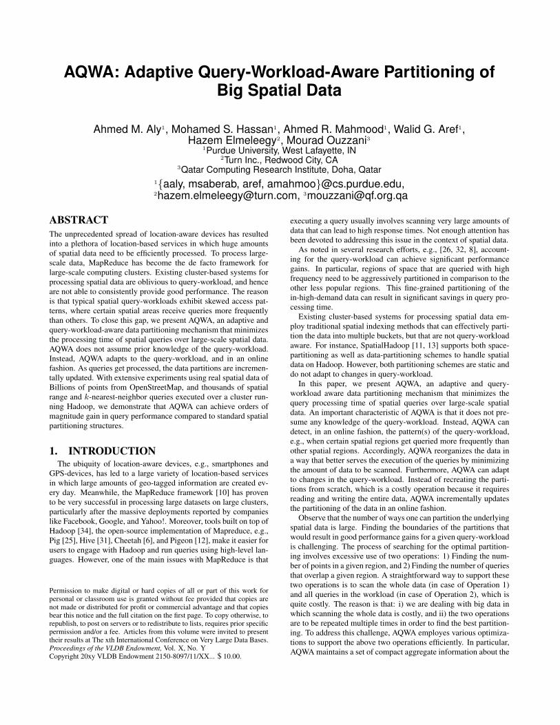
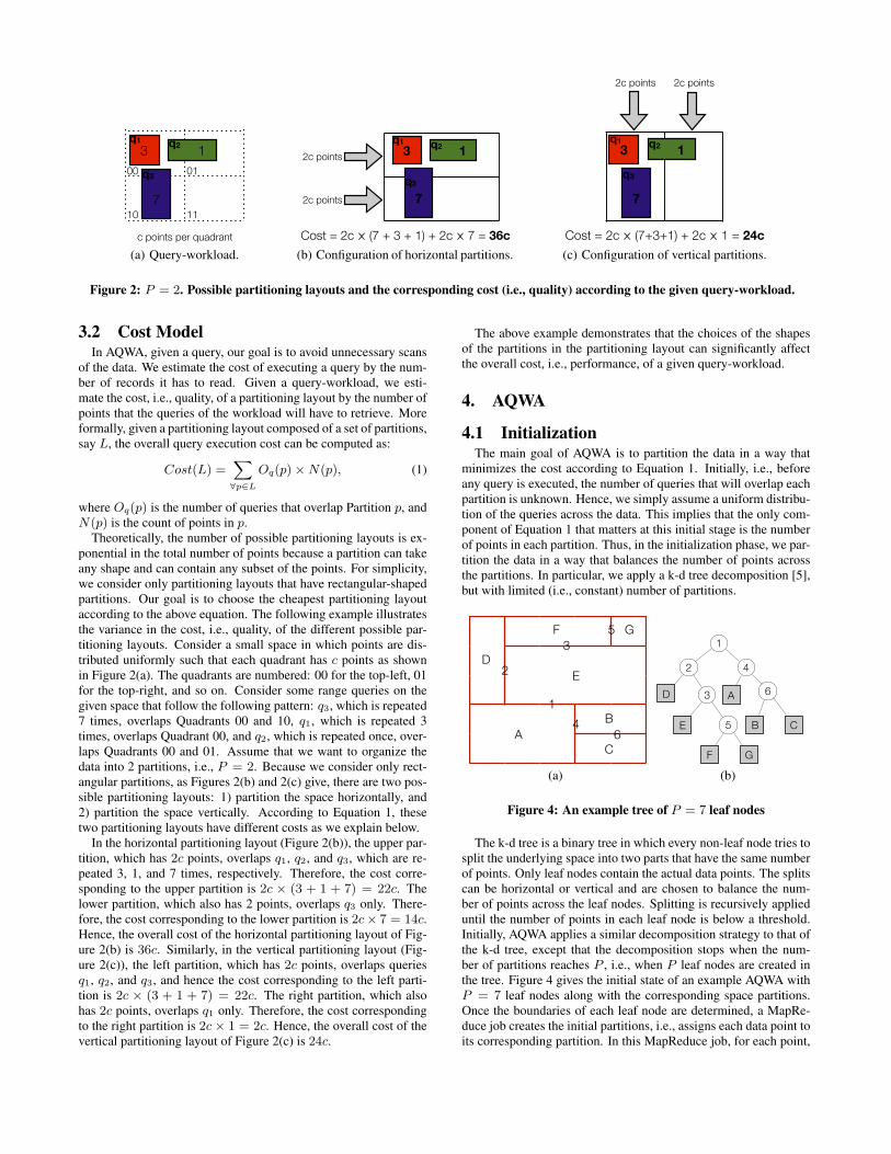
Figure 2: P = 2. Possible partitioning layouts and the corresponding cost (i.e., quality) according to the given query-workload.

3.2 Cost ModelIn AQWA, given a query, our goal is to avoid unnecessary scans

of the data. We estimate the cost of executing a query by the num-ber of records it has to read. Given a query-workload, we esti-mate the cost, i.e., quality, of a partitioning layout by the number ofpoints that the queries of the workload will have to retrieve. Moreformally, given a partitioning layout composed of a set of partitions,say L, the overall query execution cost can be computed as:

Cost(L) =∑∀p∈L

Oq(p)×N(p), (1)

where Oq(p) is the number of queries that overlap Partition p, andN(p) is the count of points in p.

Theoretically, the number of possible partitioning layouts is ex-ponential in the total number of points because a partition can takeany shape and can contain any subset of the points. For simplicity,we consider only partitioning layouts that have rectangular-shapedpartitions. Our goal is to choose the cheapest partitioning layoutaccording to the above equation. The following example illustratesthe variance in the cost, i.e., quality, of the different possible par-titioning layouts. Consider a small space in which points are dis-tributed uniformly such that each quadrant has c points as shownin Figure 2(a). The quadrants are numbered: 00 for the top-left, 01for the top-right, and so on. Consider some range queries on thegiven space that follow the following pattern: q3, which is repeated7 times, overlaps Quadrants 00 and 10, q1, which is repeated 3times, overlaps Quadrant 00, and q2, which is repeated once, over-laps Quadrants 00 and 01. Assume that we want to organize thedata into 2 partitions, i.e., P = 2. Because we consider only rect-angular partitions, as Figures 2(b) and 2(c) give, there are two pos-sible partitioning layouts: 1) partition the space horizontally, and2) partition the space vertically. According to Equation 1, thesetwo partitioning layouts have different costs as we explain below.

In the horizontal partitioning layout (Figure 2(b)), the upper par-tition, which has 2c points, overlaps q1, q2, and q3, which are re-peated 3, 1, and 7 times, respectively. Therefore, the cost corre-sponding to the upper partition is 2c × (3 + 1 + 7) = 22c. Thelower partition, which also has 2 points, overlaps q3 only. There-fore, the cost corresponding to the lower partition is 2c× 7 = 14c.Hence, the overall cost of the horizontal partitioning layout of Fig-ure 2(b) is 36c. Similarly, in the vertical partitioning layout (Fig-ure 2(c)), the left partition, which has 2c points, overlaps queriesq1, q2, and q3, and hence the cost corresponding to the left parti-tion is 2c × (3 + 1 + 7) = 22c. The right partition, which alsohas 2c points, overlaps q1 only. Therefore, the cost correspondingto the right partition is 2c× 1 = 2c. Hence, the overall cost of thevertical partitioning layout of Figure 2(c) is 24c.

The above example demonstrates that the choices of the shapesof the partitions in the partitioning layout can significantly affectthe overall cost, i.e., performance, of a given query-workload.

4. AQWA

4.1 InitializationThe main goal of AQWA is to partition the data in a way that

minimizes the cost according to Equation 1. Initially, i.e., beforeany query is executed, the number of queries that will overlap eachpartition is unknown. Hence, we simply assume a uniform distribu-tion of the queries across the data. This implies that the only com-ponent of Equation 1 that matters at this initial stage is the numberof points in each partition. Thus, in the initialization phase, we par-tition the data in a way that balances the number of points acrossthe partitions. In particular, we apply a k-d tree decomposition [5],but with limited (i.e., constant) number of partitions.

/ 79

k-d Tree Variant

19x

y

Split one cell at a time

Stop when there are k partitions

1

2

3

4

5

6A

B

C

D

E

F G

(a)/ 79

k-d Tree Variant

19

1

2

D A

B C

F G

E

3

5

4

6

(b)

Figure 4: An example tree of P = 7 leaf nodes

The k-d tree is a binary tree in which every non-leaf node tries tosplit the underlying space into two parts that have the same numberof points. Only leaf nodes contain the actual data points. The splitscan be horizontal or vertical and are chosen to balance the num-ber of points across the leaf nodes. Splitting is recursively applieduntil the number of points in each leaf node is below a threshold.Initially, AQWA applies a similar decomposition strategy to that ofthe k-d tree, except that the decomposition stops when the num-ber of partitions reaches P , i.e., when P leaf nodes are created inthe tree. Figure 4 gives the initial state of an example AQWA withP = 7 leaf nodes along with the corresponding space partitions.Once the boundaries of each leaf node are determined, a MapRe-duce job creates the initial partitions, i.e., assigns each data point toits corresponding partition. In this MapReduce job, for each point,

/ 79

Number of points in p

47

+ + + ++ + + ++ + + ++ + + ++ + + ++ + + ++ + + ++ + + +

++++++++

(a) Horizontal aggregation. / 79

Number of points in p

48

+++

+

+

+++

+

+

+++

+

+

+++

+

+

+++

+

+

+++

+

+

+++

+

+

+++

+

+

(b) Vertical aggregation. / 79

Number of points in p

49

Sum

(c) Sum after aggregation. / 79

Number of points in p

55

+

+

-

-

O(1) p

(b, r)

(t, l)

(d) O(1) lookups.

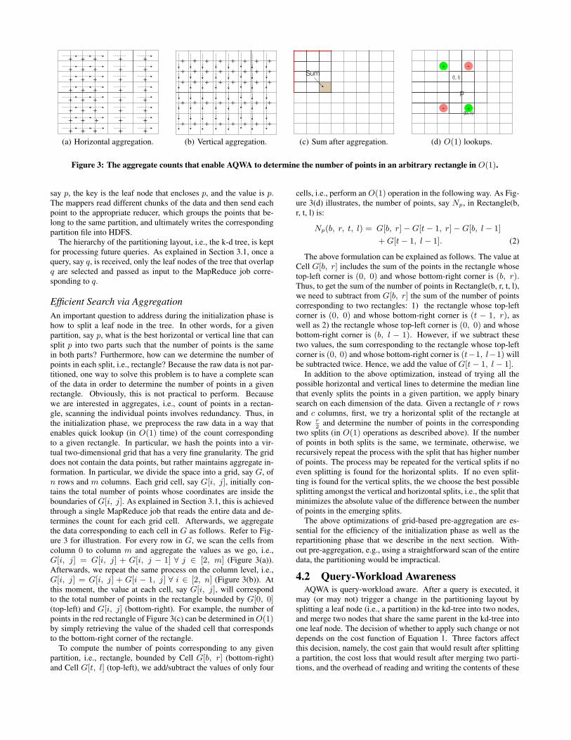
Figure 3: The aggregate counts that enable AQWA to determine the number of points in an arbitrary rectangle in O(1).

say p, the key is the leaf node that encloses p, and the value is p.The mappers read different chunks of the data and then send eachpoint to the appropriate reducer, which groups the points that be-long to the same partition, and ultimately writes the correspondingpartition file into HDFS.

The hierarchy of the partitioning layout, i.e., the k-d tree, is keptfor processing future queries. As explained in Section 3.1, once aquery, say q, is received, only the leaf nodes of the tree that overlapq are selected and passed as input to the MapReduce job corre-sponding to q.

Efficient Search via AggregationAn important question to address during the initialization phase ishow to split a leaf node in the tree. In other words, for a givenpartition, say p, what is the best horizontal or vertical line that cansplit p into two parts such that the number of points is the samein both parts? Furthermore, how can we determine the number ofpoints in each split, i.e., rectangle? Because the raw data is not par-titioned, one way to solve this problem is to have a complete scanof the data in order to determine the number of points in a givenrectangle. Obviously, this is not practical to perform. Becausewe are interested in aggregates, i.e., count of points in a rectan-gle, scanning the individual points involves redundancy. Thus, inthe initialization phase, we preprocess the raw data in a way thatenables quick lookup (in O(1) time) of the count correspondingto a given rectangle. In particular, we hash the points into a vir-tual two-dimensional grid that has a very fine granularity. The griddoes not contain the data points, but rather maintains aggregate in-formation. In particular, we divide the space into a grid, say G, ofn rows and m columns. Each grid cell, say G[i, j], initially con-tains the total number of points whose coordinates are inside theboundaries of G[i, j]. As explained in Section 3.1, this is achievedthrough a single MapReduce job that reads the entire data and de-termines the count for each grid cell. Afterwards, we aggregatethe data corresponding to each cell in G as follows. Refer to Fig-ure 3 for illustration. For every row in G, we scan the cells fromcolumn 0 to column m and aggregate the values as we go, i.e.,G[i, j] = G[i, j] + G[i, j − 1] ∀ j ∈ [2, m] (Figure 3(a)).Afterwards, we repeat the same process on the column level, i.e.,G[i, j] = G[i, j] + G[i − 1, j] ∀ i ∈ [2, n] (Figure 3(b)). Atthis moment, the value at each cell, say G[i, j], will correspondto the total number of points in the rectangle bounded by G[0, 0](top-left) and G[i, j] (bottom-right). For example, the number ofpoints in the red rectangle of Figure 3(c) can be determined in O(1)by simply retrieving the value of the shaded cell that correspondsto the bottom-right corner of the rectangle.

To compute the number of points corresponding to any givenpartition, i.e., rectangle, bounded by Cell G[b, r] (bottom-right)and Cell G[t, l] (top-left), we add/subtract the values of only four

cells, i.e., perform an O(1) operation in the following way. As Fig-ure 3(d) illustrates, the number of points, say Np, in Rectangle(b,r, t, l) is:

Np(b, r, t, l) = G[b, r]−G[t− 1, r]−G[b, l − 1]

+G[t− 1, l − 1]. (2)

The above formulation can be explained as follows. The value atCell G[b, r] includes the sum of the points in the rectangle whosetop-left corner is (0, 0) and whose bottom-right corner is (b, r).Thus, to get the sum of the number of points in Rectangle(b, r, t, l),we need to subtract from G[b, r] the sum of the number of pointscorresponding to two rectangles: 1) the rectangle whose top-leftcorner is (0, 0) and whose bottom-right corner is (t − 1, r), aswell as 2) the rectangle whose top-left corner is (0, 0) and whosebottom-right corner is (b, l − 1). However, if we subtract thesetwo values, the sum corresponding to the rectangle whose top-leftcorner is (0, 0) and whose bottom-right corner is (t−1, l−1) willbe subtracted twice. Hence, we add the value of G[t− 1, l − 1].

In addition to the above optimization, instead of trying all thepossible horizontal and vertical lines to determine the median linethat evenly splits the points in a given partition, we apply binarysearch on each dimension of the data. Given a rectangle of r rowsand c columns, first, we try a horizontal split of the rectangle atRow r

2and determine the number of points in the corresponding

two splits (in O(1) operations as described above). If the numberof points in both splits is the same, we terminate, otherwise, werecursively repeat the process with the split that has higher numberof points. The process may be repeated for the vertical splits if noeven splitting is found for the horizontal splits. If no even split-ting is found for the vertical splits, the we choose the best possiblesplitting amongst the vertical and horizontal splits, i.e., the split thatminimizes the absolute value of the difference between the numberof points in the emerging splits.

The above optimizations of grid-based pre-aggregation are es-sential for the efficiency of the initialization phase as well as therepartitioning phase that we describe in the next section. With-out pre-aggregation, e.g., using a straightforward scan of the entiredata, the partitioning would be impractical.

4.2 Query­Workload AwarenessAQWA is query-workload aware. After a query is executed, it

may (or may not) trigger a change in the partitioning layout bysplitting a leaf node (i.e., a partition) in the kd-tree into two nodes,and merge two nodes that share the same parent in the kd-tree intoone leaf node. The decision of whether to apply such change or notdepends on the cost function of Equation 1. Three factors affectthis decision, namely, the cost gain that would result after splittinga partition, the cost loss that would result after merging two parti-tions, and the overhead of reading and writing the contents of these

partitions. Below, we explain each of these factors in detail.

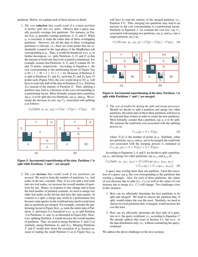
1. The cost reduction that would result if a certain partitionis further split into two splits. Observe that a query usu-ally partially overlaps few partitions. For instance, in Fig-ure 5(a), q1 partially overlaps partitions A, D, and E. Whenq1 is executed, it reads the entire data of these overlappingpartitions. However, not all the data in these overlappingpartitions is relevant, i.e., there are some points that are re-dundantly scanned in the map phase of the MapReduce jobcorresponding to q1. Thus, it would be beneficial w.r.t. q1 tofurther decompose, i.e., split, Partitions A, D, and E so thatthe amount of irrelevant data to be scanned is minimized. Forexample, assume that Partitions A, E, and D contain 20, 30,and 15 points, respectively. According to Equation 1, thecost corresponding to the partitioning layout of Figure 5(a)is 20× 1 + 30× 1 + 15× 1 = 65. However, if Partition Eis split to Partitions E1 and E2, such that E1 and E2 have 15points each (Figure 5(b)), the cost would drop to 50; q1 willhave to read only half of the data in Partition E (i.e., PartitionE2) instead of the entirety of Partition E. Thus, splitting apartition may lead to a decrease in the cost corresponding toa partitioning layout. More formally, assume that a partition,say p, is to be split into two Partitions, say p1 and p2. We es-timate the decrease in cost, say Cd, associated with splittingp as follows:

Cd(Split, p, p1, p2) = C(p)− C(p1)− C(p2). (3)

/ 79

k-d Tree Variant

20x

y

Split one cell at a time

Stop when there are k partitions

A

B

C

D

E

F G

q1

(a) / 79

k-d Tree Variant

21x

y

Split one cell at a time

Stop when there are k partitions

A BC

D E1

F G

q1 E2

(b)

Figure 5: Incremental repartitioning of the data. Partition E issplit while Partitions B and C are merged.

2. The cost increase that would result if two partitions aremerged. We need to keep the number of partitions, i.e., leafnodes in the tree, constant. Thus, if we ever split a leaf nodeinto two leaf nodes, we increase the overall number of parti-tions by one. Hence, in response to this change and to keepthe total number of partition constant, we need to merge twoother leaf nodes in the kd-tree that have the same parent. Incontrast to a split, a merge may result in a performance lossbecause some queries in the workload may need to read moredata as partitions get merged. For example, consider the par-titioning layout in Figure 6(a). q3 reads the entire data of Par-tition A, and hence it is beneficial w.r.t. q3 to split PartitionA to Partitions A1 and A2 as illustrated in Figure 6(b). How-ever, splitting Partition A would increase the overall numberof partitions. Thus, we need to merge Partitions F and G (orsimilarly, merge Partitions E1 and E2). Merging PartitionsF and G would slow down the execution of q2 because in-stead of reading the small Partition G as in Figure 6(a), q2

will have to read the entirety of the merged partition, i.e.,Partition FG. Thus, merging two partitions may lead to anincrease in the cost corresponding to a partitioning layout.Similarly to Equation 3, we estimate the cost loss, say Ci,associated with merging two partitions, say p1 and p2, into asingle partition, say p as:

Ci(Merge, p1, p2, p) = C(p)− C(p1)− C(p2). (4)

/ 79

k-d Tree Variant

22x

y

Split one cell at a time

Stop when there are k partitions

A BC

D E1

F G

q1 E2

q2

q3

(a) / 79

k-d Tree Variant

23x

y

Split one cell at a time

Stop when there are k partitions

A1 BC

D E1

FG

q1E2

q2

q3

A2

(b)

Figure 6: Incremental repartitioning of the data. Partition A issplit while Partitions F and G are merged.

3. The cost of read/write during the split and merge processes.Should we decide to split a partition and merge two otherpartitions, the entire data of these three partitions will have tobe read and then written in order to create the new partitions.More formally, assume that a partition, say p, is to be split.We estimate the read/write cost associated with the splittingprocess as:

Crw(p) = 2×N(p), (5)

where N(p) is the number of points in p. Similarly, whentwo partitions, say p1 and p2, are to be merged, the read/writecost associated with the merging process is estimated asCrw(p1, p2) = 2×N(p1) + 2×N(p2).

According to Equations 3, 4, and 5, we decide to split a partition,say ps, and merge two other partitions, say pm1 and pm2 if:

Cd(Split, ps, ps1, ps2) > [Ci(Merge, pm1, pm2, pm)

+ Crw(ps) + Crw(pm1, pm2)]. (6)

A query may overlap more than one partition. Upon the execu-tion of a query, say q, the cost corresponding to the partitions thatoverlap q changes. Also, for each of these partitions, the valuesof cost decrease due to split (i.e., Cd) as well as the values of costincrease due to merge (i.e., Ci) will change. Two challenges existin this situation:

1. How can we efficiently determine the best partitions to besplit and merged? We need to choose the partition that, ifsplit, would reduce the cost the most. Similarly, we need tochoose two leaf partitions that, if merged, would increase thecost the least.

2. How can we efficiently determine the best split of a parti-tion w.r.t. the query-workload, i.e., according to Equation 1?We already address this issue in Section 4.1, but w.r.t. tothe data distribution only, i.e., without considering the query-workload.

We address the above challenges in the next sections.

/ 7945

Proposed Solution (Invariant)

min-heap

max-heap

Merge Performance-Loss: Split Performance-Gain:

>Invariant

Cd(Ps) - 2⨉N(Ps)Ci(Pm1, Pm2) - 2⨉[N(Pm1)+N(Pm2)]

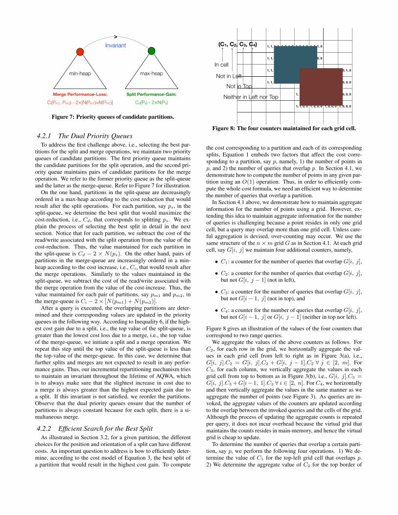
Figure 7: Priority queues of candidate partitions.

4.2.1 The Dual Priority QueuesTo address the first challenge above, i.e., selecting the best par-

titions for the split and merge operations, we maintain two priorityqueues of candidate partitions. The first priority queue maintainsthe candidate partitions for the split operation, and the second pri-ority queue maintains pairs of candidate partitions for the mergeoperation. We refer to the former priority queue as the split-queueand the latter as the merge-queue. Refer to Figure 7 for illustration.

On the one hand, partitions in the split-queue are decreasinglyordered in a max-heap according to the cost reduction that wouldresult after the split operations. For each partition, say ps, in thesplit-queue, we determine the best split that would maximize thecost-reduction, i.e., Cd, that corresponds to splitting ps. We ex-plain the process of selecting the best split in detail in the nextsection. Notice that for each partition, we subtract the cost of theread/write associated with the split operation from the value of thecost-reduction. Thus, the value maintained for each partition inthe split-queue is Cd − 2 × N(ps). On the other hand, pairs ofpartitions in the merge-queue are increasingly ordered in a min-heap according to the cost increase, i.e., Ci, that would result afterthe merge operations. Similarly to the values maintained in thesplit-queue, we subtract the cost of the read/write associated withthe merge operation from the value of the cost-increase. Thus, thevalue maintained for each pair of partitions, say pm1 and pm2, inthe merge-queue is Ci − 2× [N(pm1) +N(pm2)].

After a query is executed, the overlapping partitions are deter-mined and their corresponding values are updated in the priorityqueues in the following way. According to Inequality 6, if the high-est cost gain due to a split, i.e., the top value of the split-queue, isgreater than the lowest cost loss due to a merge, i.e., the top valueof the merge-queue, we initiate a split and a merge operation. Werepeat this step until the top value of the split-queue is less thanthe top-value of the merge-queue. In this case, we determine thatfurther splits and merges are not expected to result in any perfor-mance gains. Thus, our incremental repartitioning mechanism triesto maintain an invariant throughout the lifetime of AQWA, whichis to always make sure that the slightest increase in cost due toa merge is always greater than the highest expected gain due toa split. If this invariant is not satisfied, we reorder the partitions.Observe that the dual priority queues ensure that the number ofpartitions is always constant because for each split, there is a si-multaneous merge.

4.2.2 Efficient Search for the Best SplitAs illustrated in Section 3.2, for a given partition, the different

choices for the position and orientation of a split can have differentcosts. An important question to address is how to efficiently deter-mine, according to the cost model of Equation 3, the best split ofa partition that would result in the highest cost gain. To compute

/ 79

Number of regions Overlapping with pInserting a region

66

1, 1, 1, 1 1, 0, 1, 0 1, 0, 1, 0 1, 0, 1, 0

1, 1, 0, 0 1, 0, 0, 0 1, 0, 0, 0 1, 0, 0, 0

1, 1, 0, 0 1, 0, 0, 0 2, 1, 1, 1 2, 0, 1, 0 1, 0, 1, 0 1, 0, 1, 0

1, 1, 0, 0 1, 0, 0, 0 2, 1, 0, 0 2, 0, 0, 0 1, 0, 0, 0 1, 0, 0, 0

1, 1, 0, 0 1, 0, 0, 0 1, 0, 0, 0 1, 0, 0, 0

1, 1, 0, 0 1, 0, 0, 0 1, 0, 0, 0 1, 0, 0, 0

(C1, C2, C3, C4)

In cell

Not in Left

Not in Top

Neither in Left nor Top

Figure 8: The four counters maintained for each grid cell.

the cost corresponding to a partition and each of its correspondingsplits, Equation 1 embeds two factors that affect the cost corre-sponding to a partition, say p, namely, 1) the number of points inp, and 2) the number of queries that overlap p. In Section 4.1, wedemonstrate how to compute the number of points in any given par-tition using an O(1) operation. Thus, in order to efficiently com-pute the whole cost formula, we need an efficient way to determinethe number of queries that overlap a partition.

In Section 4.1 above, we demonstrate how to maintain aggregateinformation for the number of points using a grid. However, ex-tending this idea to maintain aggregate information for the numberof queries is challenging because a point resides in only one gridcell, but a query may overlap more than one grid cell. Unless care-ful aggregation is devised, over-counting may occur. We use thesame structure of the n×m grid G as in Section 4.1. At each gridcell, say G[i, j] we maintain four additional counters, namely,

• C1: a counter for the number of queries that overlap G[i, j],

• C2: a counter for the number of queries that overlap G[i, j],but not G[i, j − 1] (not in left),

• C3: a counter for the number of queries that overlap G[i, j],but not G[i− 1, j] (not in top), and

• C4: a counter for the number of queries that overlap G[i, j],but not G[i− 1, j] or G[i, j − 1] (neither in top nor left).

Figure 8 gives an illustration of the values of the four counters thatcorrespond to two range queries.

We aggregate the values of the above counters as follows. ForC2, for each row in the grid, we horizontally aggregate the val-ues in each grid cell from left to right as in Figure 3(a), i.e.,G[i, j].C2 = G[i, j].C2 + G[i, j − 1].C2 ∀ j ∈ [2, m]. ForC3, for each column, we vertically aggregate the values in eachgrid cell from top to bottom as in Figure 3(b), i.e., G[i, j].C3 =G[i, j].C3 +G[i− 1, 1].C3 ∀ i ∈ [2, n]. For C4, we horizontallyand then vertically aggregate the values in the same manner as weaggregate the number of points (see Figure 3). As queries are in-voked, the aggregate values of the counters are updated accordingto the overlap between the invoked queries and the cells of the grid.Although the process of updating the aggregate counts is repeatedper query, it does not incur overhead because the virtual grid thatmaintains the counts resides in main-memory, and hence the virtualgrid is cheap to update.

To determine the number of queries that overlap a certain parti-tion, say p, we perform the following four operations. 1) We de-termine the value of C1 for the top-left grid cell that overlaps p.2) We determine the aggregate value of C2 for the top border of

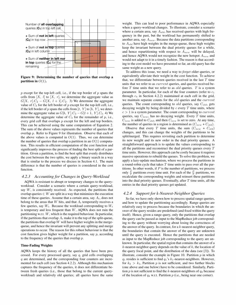
/ 79

Finding the Number of Regions Overlapping with p

71

Number of all overlapping queries (C1) in top left cell

+ Sum of not in left queries (C2) in top row

+ Sum of not in top queries (C3) in left column

+ Sum of neither in left nor in top queries (C4) for the remaining

Figure 9: Determining the number of queries that overlap apartition in O(1).

p except for the top-left cell, i.e., if the top border of p spans thecells from [X, l] to [X, r], we determine the aggregate value asG[X, r].C2 − G[X, l + 1].C2. 3) We determine the aggregatevalue of C3 for the left border of p except for the top-left cell, i.e.,if the left border of p spans the cells from [t, Y ] to [b, Y ], we deter-mine the aggregate value as G[b, Y ].C3 −G[t+1, Y ].C3. 4) Wedetermine the aggregate value of C4 for the remainder of p, i.e.,every grid cell that overlaps p except for the left and top borders.This can be achieved using the same computation of Equation 2.The sum of the above values represents the number of queries thatoverlap p. Refer to Figure 9 for illustration. Observe that each ofthe above values is computed in O(1). Thus, we can determinethe number of queries that overlap a partition in an O(1) computa-tion. This results in efficient computation of the cost function andsignificantly improves the process of finding the best split of a par-tition. Given a partition, to find the best split that evenly distributesthe cost between the two splits, we apply a binary search in a waythat is similar to the process we discuss in Section 4.1. The maindifference is that the number of queries is considered in the costfunction.

4.2.3 Accounting for Changes in Query­WorkloadAQWA is resistant to abrupt or temporary changes to the query-

workload. Consider a scenario where a certain query-workload,say W , is consistently received. As expected, the partitions thatoverlap queries ∈ W are split in a way that minimizes the executiontime of these queries. Assume that a certain area, say At, does notbelong to the areas that W hits, and that At temporarily receives afew queries, say Wt. Because the workload corresponding to Wt

is temporary and less frequent than W , AQWA does not ruin thepartitioning w.r.t. W , which is the required behaviour. In particular,if the partitions that overlap At make it to the top of the split-queue,the partitions that overlap W will have higher weights in the merge-queue, and hence the invariant will prevent any splitting and mergeoperations to occur. The reason for this robust behaviour is that thecost function gives higher weight for a partition, say p, accordingto the frequency of the queries that overlap p.

Time-Fading WeightsAQWA keeps the history of all the queries that have been pro-cessed. For every processed query, say q, grid cells overlappingq are determined, and the corresponding four counters are incre-mented for each cell (see Section 4.2.2). Although this mechanismcaptures the frequency of the queries, it does not differentiate be-tween fresh queries (i.e., those that belong to the current query-workload) and relatively old queries; all queries have the same

weight. This can lead to poor performance in AQWA especiallywhen a query-workload changes. To illustrate, consider a scenariowhere a certain area, say Aold, has received queries with high fre-quency in the past, but the workload has permanently shifted toanother area, say Anew. Because the data partitions correspondingto Aold have high weights in the merge-queue, these high weightskeep the invariant between the dual priority queues for a while,and hence repartitioning with respect to Anew will be delayed,and hence AQWA would not recognize the new hotspot Anew andwould not adapt to it in a timely fashion. The reason is that accord-ing to the cost model we have presented so far, an old query has thesame weight as a new query.

To address this issue, we need a way to forget older queries, orequivalently alleviate their weight in the cost function. To achievethat, we differentiate between queries received in the last T timeunits that we refer to as current queries, and queries received be-fore T time units that we refer to as old queries. T is a systemparameter. In particular, for each of the four counters (refer to c1through c4 in Section 4.2.2) maintained at each cell in the grid,we maintain separate counts for the old queries and the currentqueries. The count corresponding to old queries, say Cold, getsdecaying weight by being divided by c every T time units, wherec > 1 is a system parameter. The count corresponding to currentqueries, say Cnew, has no decaying weight. Every T time units,Cnew is added to Cold, and then Cnew is set to zero. At any time,the number of queries in a region is determined as (Cnew + Cold).

Observe that every T time units, the sum (Cnew + Cold)changes, and this can change the weights of the partitions to besplit/merged. This requires revisiting each partition to determineits new weight and its new order in the dual priority queues. Astraightforward approach is to update the values corresponding toall the partitions and reconstruct the dual priority queues every Ttime units. However, this approach can be costly because it requiresmassive operations to rebuild the queues. To solve this problem, weapply a lazy-update mechanism, where we process the partitions ina round-robin cycle that takes T time units to pass over all the par-titions. In other words, if P is the number of partitions, we processonly P

Tpartitions every time unit. For each of the P

Tpartitions, we

recalculate the corresponding weights and reinsert these partitionsinto the dual priority queues. Eventually, after T time units, all theentries in the dual priority queues get updated.

4.2.4 Support for k­Nearest­Neighbor QueriesSo far, we have only shown how to process spatial range queries,

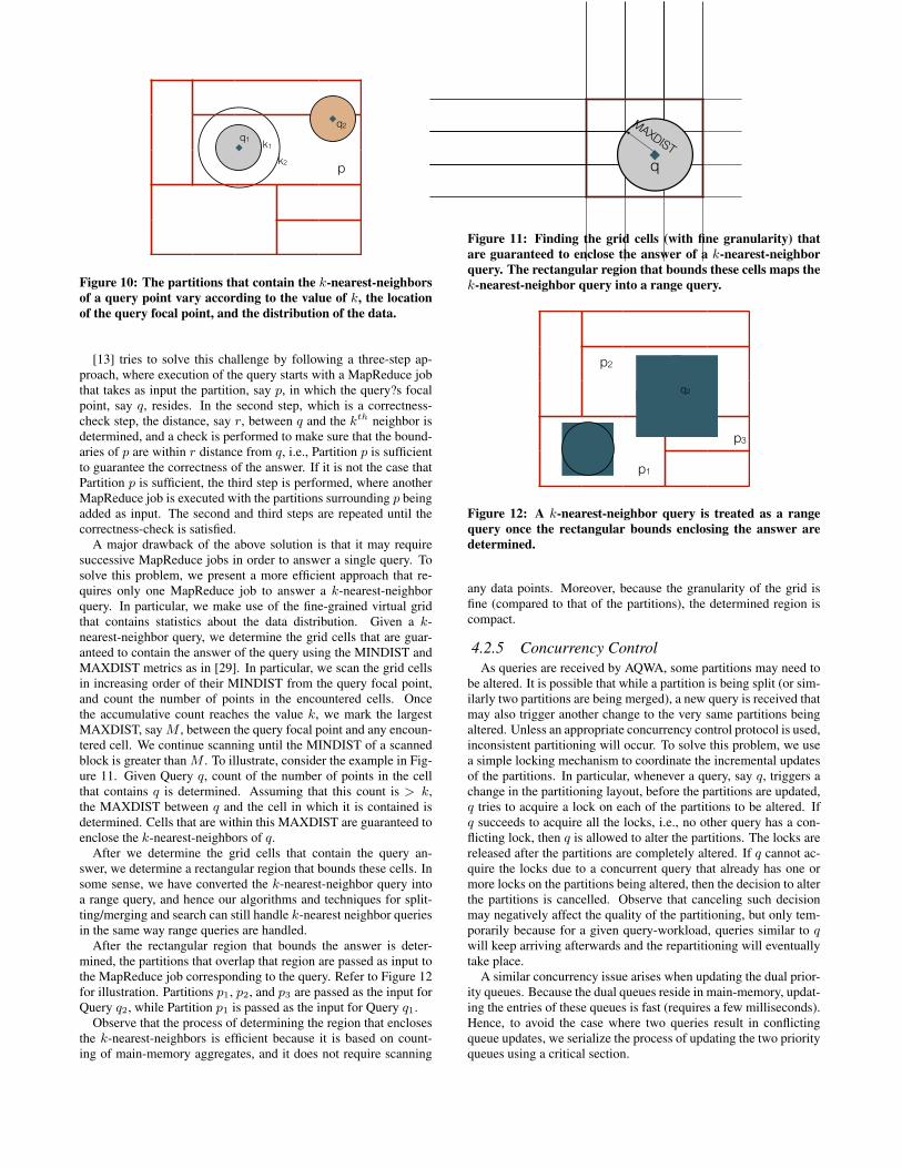
and how to update the partitioning accordingly. Range queries arerelatively easy to process because the boundaries in which the an-swer of the query resides are predefined (and fixed within the queryitself). Hence, given a range query, only the partitions that overlapthe query can be passed as input to the MapReduce job correspond-ing to the query without worrying about losing the correctness ofthe answer of the query. In contrast, for a k-nearest-neighbor query,the boundaries that contain the answer of the query are unknownuntil the query is executed. Hence the partitions that are neededas input to the MapReduce job corresponding to the query are un-known. In particular, the spatial region that contains the answer of ak-nearest-neighbor query depends on the value of k, the location ofthe query focal point, and the distribution of the data (see [3]). Toillustrate, consider the example in Figure 10. Partition p in whichq1 resides is sufficient to find q1’s k1-nearest-neighbors. However,for k2 > k1, Partition p is not sufficient, and two further blocks(one above and one below) have to be considered. Similarly, Parti-tion p is not sufficient to find the k-nearest-neighbors of q2 becauseof the location of q2 w.r.t. Partition p (i.e., being near one corner).

/ 796

AQWA - Support for kNN Queries

k1

k2

q1

q2

p

Figure 10: The partitions that contain the k-nearest-neighborsof a query point vary according to the value of k, the locationof the query focal point, and the distribution of the data.

[13] tries to solve this challenge by following a three-step ap-proach, where execution of the query starts with a MapReduce jobthat takes as input the partition, say p, in which the query?s focalpoint, say q, resides. In the second step, which is a correctness-check step, the distance, say r, between q and the kth neighbor isdetermined, and a check is performed to make sure that the bound-aries of p are within r distance from q, i.e., Partition p is sufficientto guarantee the correctness of the answer. If it is not the case thatPartition p is sufficient, the third step is performed, where anotherMapReduce job is executed with the partitions surrounding p beingadded as input. The second and third steps are repeated until thecorrectness-check is satisfied.

A major drawback of the above solution is that it may requiresuccessive MapReduce jobs in order to answer a single query. Tosolve this problem, we present a more efficient approach that re-quires only one MapReduce job to answer a k-nearest-neighborquery. In particular, we make use of the fine-grained virtual gridthat contains statistics about the data distribution. Given a k-nearest-neighbor query, we determine the grid cells that are guar-anteed to contain the answer of the query using the MINDIST andMAXDIST metrics as in [29]. In particular, we scan the grid cellsin increasing order of their MINDIST from the query focal point,and count the number of points in the encountered cells. Oncethe accumulative count reaches the value k, we mark the largestMAXDIST, say M , between the query focal point and any encoun-tered cell. We continue scanning until the MINDIST of a scannedblock is greater than M . To illustrate, consider the example in Fig-ure 11. Given Query q, count of the number of points in the cellthat contains q is determined. Assuming that this count is > k,the MAXDIST between q and the cell in which it is contained isdetermined. Cells that are within this MAXDIST are guaranteed toenclose the k-nearest-neighbors of q.

After we determine the grid cells that contain the query an-swer, we determine a rectangular region that bounds these cells. Insome sense, we have converted the k-nearest-neighbor query intoa range query, and hence our algorithms and techniques for split-ting/merging and search can still handle k-nearest neighbor queriesin the same way range queries are handled.

After the rectangular region that bounds the answer is deter-mined, the partitions that overlap that region are passed as input tothe MapReduce job corresponding to the query. Refer to Figure 12for illustration. Partitions p1, p2, and p3 are passed as the input forQuery q2, while Partition p1 is passed as the input for Query q1.

Observe that the process of determining the region that enclosesthe k-nearest-neighbors is efficient because it is based on count-ing of main-memory aggregates, and it does not require scanning

/ 79

AQWA - Support for kNN Queries

8

MINDISTScan &

Counting

MAXDIST

q

Figure 11: Finding the grid cells (with fine granularity) thatare guaranteed to enclose the answer of a k-nearest-neighborquery. The rectangular region that bounds these cells maps thek-nearest-neighbor query into a range query.

/ 799

AQWA - Support for kNN Queries

It’s not a map-only jobCan we ignore communication cost?

q1

q2

p2

p1

p3

Figure 12: A k-nearest-neighbor query is treated as a rangequery once the rectangular bounds enclosing the answer aredetermined.

any data points. Moreover, because the granularity of the grid isfine (compared to that of the partitions), the determined region iscompact.

4.2.5 Concurrency ControlAs queries are received by AQWA, some partitions may need to

be altered. It is possible that while a partition is being split (or sim-ilarly two partitions are being merged), a new query is received thatmay also trigger another change to the very same partitions beingaltered. Unless an appropriate concurrency control protocol is used,inconsistent partitioning will occur. To solve this problem, we usea simple locking mechanism to coordinate the incremental updatesof the partitions. In particular, whenever a query, say q, triggers achange in the partitioning layout, before the partitions are updated,q tries to acquire a lock on each of the partitions to be altered. Ifq succeeds to acquire all the locks, i.e., no other query has a con-flicting lock, then q is allowed to alter the partitions. The locks arereleased after the partitions are completely altered. If q cannot ac-quire the locks due to a concurrent query that already has one ormore locks on the partitions being altered, then the decision to alterthe partitions is cancelled. Observe that canceling such decisionmay negatively affect the quality of the partitioning, but only tem-porarily because for a given query-workload, queries similar to qwill keep arriving afterwards and the repartitioning will eventuallytake place.

A similar concurrency issue arises when updating the dual prior-ity queues. Because the dual queues reside in main-memory, updat-ing the entries of these queues is fast (requires a few milliseconds).Hence, to avoid the case where two queries result in conflictingqueue updates, we serialize the process of updating the two priorityqueues using a critical section.

5. EXPERIMENTSIn this section, we evaluate the performance of AQWA. We real-

ize a cluster-based test bed in which we implement AQWA as wellas the uniform grid and a static k-d tree partitioning. We choosethese two structures because we want to contrast the performance ofAQWA against two different extreme partitioning schemes: 1) purespatial decomposition, i.e., when using a Grid, and 2) data decom-position, i.e., when using a k-d tree. Experiments are conducted ona 16-node cluster running Hadoop over Red Hat Enterprise Linux6.4. Each node in the cluster has four 1TB hard drives, 8GB ofRAM, and 4 cores Intel(R) Xeon(R) E31240 @3.30GHz. Thenodes of the cluster are all connected with 1Gbps networking.

We use a real spatial dataset from OpenStreetMap [1]. The num-ber of data points in the dataset is 2.7 Billion points. The format ofeach point is simply comma-separated longitude-latitude. We usevarious query-workloads that were selected to follow the spatialdistribution of the data. The intuition behind selecting the query-workload is that certain areas that have high density are likely toreceive more queries than less dense areas. Hence, we generated10 different query-workloads that focus on 10 dense spatial areas.We use range and k-nearest-neighbor queries.

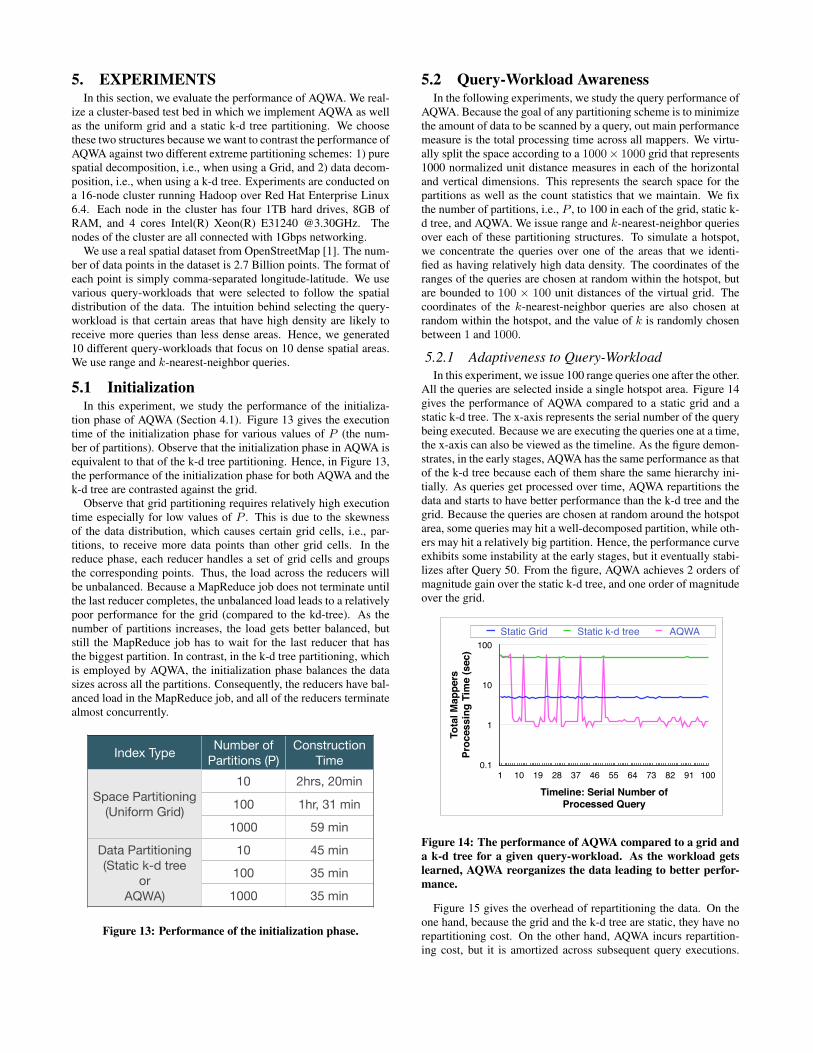
5.1 InitializationIn this experiment, we study the performance of the initializa-

tion phase of AQWA (Section 4.1). Figure 13 gives the executiontime of the initialization phase for various values of P (the num-ber of partitions). Observe that the initialization phase in AQWA isequivalent to that of the k-d tree partitioning. Hence, in Figure 13,the performance of the initialization phase for both AQWA and thek-d tree are contrasted against the grid.

Observe that grid partitioning requires relatively high executiontime especially for low values of P . This is due to the skewnessof the data distribution, which causes certain grid cells, i.e., par-titions, to receive more data points than other grid cells. In thereduce phase, each reducer handles a set of grid cells and groupsthe corresponding points. Thus, the load across the reducers willbe unbalanced. Because a MapReduce job does not terminate untilthe last reducer completes, the unbalanced load leads to a relativelypoor performance for the grid (compared to the kd-tree). As thenumber of partitions increases, the load gets better balanced, butstill the MapReduce job has to wait for the last reducer that hasthe biggest partition. In contrast, in the k-d tree partitioning, whichis employed by AQWA, the initialization phase balances the datasizes across all the partitions. Consequently, the reducers have bal-anced load in the MapReduce job, and all of the reducers terminatealmost concurrently.

/ 114

Index Construction (Initialization)

Index Type Number of Partitions (P)

Construction Time

Space Partitioning(Uniform Grid)

10 2hrs, 20min

100 1hr, 31 min

1000 59 min

Data Partitioning(Static k-d tree

or AQWA)

10 45 min

100 35 min

1000 35 min

Figure 13: Performance of the initialization phase.

5.2 Query­Workload AwarenessIn the following experiments, we study the query performance of

AQWA. Because the goal of any partitioning scheme is to minimizethe amount of data to be scanned by a query, out main performancemeasure is the total processing time across all mappers. We virtu-ally split the space according to a 1000× 1000 grid that represents1000 normalized unit distance measures in each of the horizontaland vertical dimensions. This represents the search space for thepartitions as well as the count statistics that we maintain. We fixthe number of partitions, i.e., P , to 100 in each of the grid, static k-d tree, and AQWA. We issue range and k-nearest-neighbor queriesover each of these partitioning structures. To simulate a hotspot,we concentrate the queries over one of the areas that we identi-fied as having relatively high data density. The coordinates of theranges of the queries are chosen at random within the hotspot, butare bounded to 100 × 100 unit distances of the virtual grid. Thecoordinates of the k-nearest-neighbor queries are also chosen atrandom within the hotspot, and the value of k is randomly chosenbetween 1 and 1000.

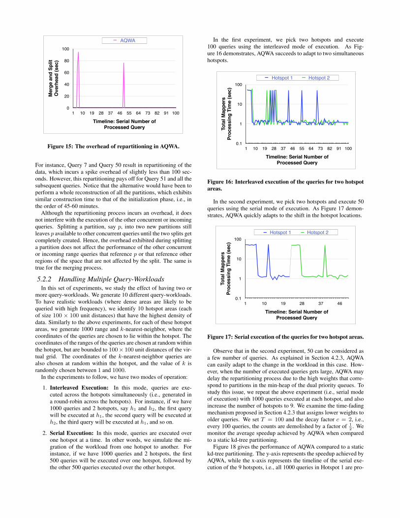
5.2.1 Adaptiveness to Query­WorkloadIn this experiment, we issue 100 range queries one after the other.

All the queries are selected inside a single hotspot area. Figure 14gives the performance of AQWA compared to a static grid and astatic k-d tree. The x-axis represents the serial number of the querybeing executed. Because we are executing the queries one at a time,the x-axis can also be viewed as the timeline. As the figure demon-strates, in the early stages, AQWA has the same performance as thatof the k-d tree because each of them share the same hierarchy ini-tially. As queries get processed over time, AQWA repartitions thedata and starts to have better performance than the k-d tree and thegrid. Because the queries are chosen at random around the hotspotarea, some queries may hit a well-decomposed partition, while oth-ers may hit a relatively big partition. Hence, the performance curveexhibits some instability at the early stages, but it eventually stabi-lizes after Query 50. From the figure, AQWA achieves 2 orders ofmagnitude gain over the static k-d tree, and one order of magnitudeover the grid.

i Grid kd Dynamic Grid kd Dynamic

1 5.126 58.437 53.591 5126 58437 535912 4.825 48.831 50.981 4825 48831 509813 5.124 49.489 49.732 5124 49489 497324 4.821 50.046 50.653 4821 50046 506535 5.125 48.237 50.08 5125 48237 500806 4.823 47.146 56.107 4823 47146 561077 4.825 49.158 1.509 4825 49158 15098 4.52 47.312 1.209 4520 47312 12099 4.826 48.841 1.207 4826 48841 120710 5.128 48.556 1.511 5128 48556 151111 4.825 48.838 1.207 4825 48838 120712 4.839 48.868 56.051 4839 48868 5605113 5.125 48.838 1.207 5125 48838 120714 4.825 48.528 1.207 4825 48528 120715 4.522 48.227 1.206 4522 48227 120616 4.822 47.928 1.207 4822 47928 120717 4.941 48.868 1.206 4941 48868 120618 4.521 48.818 0.906 4521 48818 90619 4.823 50.161 0.904 4823 50161 90420 4.823 47.954 1.509 4823 47954 150921 4.827 48.056 1.207 4827 48056 120722 4.836 49.253 1.208 4836 49253 120823 5.125 49.159 56.689 5125 49159 5668924 5.128 48.829 1.509 5128 48829 150925 4.823 48.52 1.207 4823 48520 120726 4.823 47.912 1.208 4823 47912 120827 4.821 49.126 1.509 4821 49126 150928 4.83 47.934 1.208 4830 47934 120829 4.829 48.56 51.58 4829 48560 5158030 5.123 47.64 0.907 5123 47640 90731 4.827 50.218 0.905 4827 50218 90532 4.821 48.525 1.206 4821 48525 120633 5.127 49.168 1.207 5127 49168 120734 4.822 48.387 1.207 4822 48387 120735 4.822 48.826 1.207 4822 48826 120736 4.823 49.364 1.208 4823 49364 120837 4.52 47.624 1.205 4520 47624 120538 5.238 47.978 1.207 5238 47978 120739 4.916 49.127 55.478 4916 49127 5547840 4.525 49.448 1.208 4525 49448 120841 5.126 48.829 1.51 5126 48829 151042 4.823 48.29 0.906 4823 48290 90643 4.822 47.917 1.206 4822 47917 120644 4.824 48.536 1.207 4824 48536 120745 4.821 49.372 0.905 4821 49372 90546 4.821 47.929 1.208 4821 47929 120847 5.125 49.436 1.206 5125 49436 120648 4.829 48.831 1.206 4829 48831 120649 4.825 47.06 1.207 4825 47060 120750 4.823 50.078 54.62 4823 50078 5462051 4.822 48.524 1.51 4822 48524 151052 4.826 48.235 1.554 4826 48235 155453 4.824 48.217 1.207 4824 48217 120754 4.824 47.991 1.209 4824 47991 120955 4.822 48.526 1.208 4822 48526 120856 4.825 48.837 1.209 4825 48837 120957 5.251 48.521 1.208 5251 48521 120858 4.823 49.429 1.297 4823 49429 129759 4.824 47.616 1.207 4824 47616 120760 4.823 48.888 1.336 4823 48888 133661 4.825 47.928 1.207 4825 47928 120762 4.823 48.613 1.207 4823 48613 120763 4.824 47.929 1.207 4824 47929 120764 4.825 48.64 1.207 4825 48640 120765 4.825 48.912 1.207 4825 48912 120766 5.125 48.354 1.546 5125 48354 154667 4.827 48.232 1.509 4827 48232 150968 4.52 48.899 0.906 4520 48899 90669 4.52 48.859 1.207 4520 48859 120770 4.824 48.53 1.207 4824 48530 120771 5.128 48.275 1.208 5128 48275 120872 4.821 47.621 1.206 4821 47621 120673 4.95 49.441 1.209 4950 49441 120974 4.825 48.29 1.207 4825 48290 120775 4.52 49.444 1.208 4520 49444 120876 4.825 48.538 1.207 4825 48538 120777 5.124 47.011 1.51 5124 47011 151078 4.881 48.524 1.207 4881 48524 120779 4.824 47.926 1.207 4824 47926 120780 4.825 47.947 0.906 4825 47947 90681 4.823 47.63 1.208 4823 47630 120882 4.826 48.566 1.206 4826 48566 120683 4.826 49.452 1.509 4826 49452 150984 4.826 49.124 1.508 4826 49124 150885 4.821 48.517 1.208 4821 48517 120886 4.824 49.453 1.208 4824 49453 120887 5.123 49.499 1.509 5123 49499 150988 4.823 48.82 0.906 4823 48820 90689 4.822 48.526 1.207 4822 48526 120790 4.822 49.745 0.906 4822 49745 906

HD

FS M

B R

ead

1

10

100

1000

10000

Number of Queries Processed1

Grid kd

HD

FS M

B R

ead

1

10

100

1000

10000

Number of Queries Processed1 21 41 61 81

Grid kd

Tota

l Map

pers

Pr

oces

sing

Tim

e (s

ec)

0.1

1

10

100

Timeline: Serial Number of Processed Query

1 10 19 28 37 46 55 64 73 82 91 100

Static Grid Static k-d tree AQWA

�1

Figure 14: The performance of AQWA compared to a grid anda k-d tree for a given query-workload. As the workload getslearned, AQWA reorganizes the data leading to better perfor-mance.

Figure 15 gives the overhead of repartitioning the data. On theone hand, because the grid and the k-d tree are static, they have norepartitioning cost. On the other hand, AQWA incurs repartition-ing cost, but it is amortized across subsequent query executions.

i Grid kd Dynamic Grid kd Dynamic

1 0 0 0 02 0 0 0 03 0 0 0 04 0 0 0 05 0 0 73.629 736296 0 0 94.877 948777 0 0 0 08 0 0 0 09 0 0 0 010 0 0 0 011 0 0 0 012 0 0 0 013 0 0 0 014 0 0 0 015 0 0 0 016 0 0 0 017 0 0 0 018 0 0 0 019 0 0 0 020 0 0 0 021 0 0 0 022 0 0 0 023 0 0 0 024 0 0 0 025 0 0 0 026 0 0 0 027 0 0 0 028 0 0 0 029 0 0 0 030 0 0 0 031 0 0 0 032 0 0 0 033 0 0 0 034 0 0 0 035 0 0 0 036 0 0 0 037 0 0 0 038 0 0 0 039 0 0 0 040 0 0 0 041 0 0 0 042 0 0 0 043 0 0 0 044 0 0 0 045 0 0 0 046 0 0 0 047 0 0 0 048 0 0 0 049 0 0 0 050 0 0 76.124 7612451 0 0 0 052 0 0 0 053 0 0 0 054 0 0 0 055 0 0 0 056 0 0 0 057 0 0 0 058 0 0 0 059 0 0 0 060 0 0 0 061 0 0 0 062 0 0 0 063 0 0 0 064 0 0 0 065 0 0 0 066 0 0 0 067 0 0 0 068 0 0 0 069 0 0 0 070 0 0 0 071 0 0 0 072 0 0 0 073 0 0 0 074 0 0 0 075 0 0 0 076 0 0 0 077 0 0 0 078 0 0 0 079 0 0 0 080 0 0 0 081 0 0 0 082 0 0 0 083 0 0 0 084 0 0 0 085 0 0 0 086 0 0 0 087 0 0 0 088 0 0 0 089 0 0 0 090 0 0 0 0

HDFS

MB

Read

1

10

100

1000

10000

Number of Queries Processed1

Grid kd

HDFS

MB

Read

1

10

100

1000

10000

Number of Queries Processed1 21 41 61 81

Grid kd

Mer

ge a

nd S

plit

Ove

rhea

d (s

ec)

0

20

40

60

80

100

Timeline: Serial Number ofProcessed Query

1 10 19 28 37 46 55 64 73 82 91 100

AQWA

�1

Figure 15: The overhead of repartitioning in AQWA.

For instance, Query 7 and Query 50 result in repartitioning of thedata, which incurs a spike overhead of slightly less than 100 sec-onds. However, this repartitioning pays off for Query 51 and all thesubsequent queries. Notice that the alternative would have been toperform a whole reconstruction of all the partitions, which exhibitssimilar construction time to that of the initialization phase, i.e., inthe order of 45-60 minutes.

Although the repartitioning process incurs an overhead, it doesnot interfere with the execution of the other concurrent or incomingqueries. Splitting a partition, say p, into two new partitions stillleaves p available to other concurrent queries until the two splits getcompletely created. Hence, the overhead exhibited during splittinga partition does not affect the performance of the other concurrentor incoming range queries that reference p or that reference otherregions of the space that are not affected by the split. The same istrue for the merging process.

5.2.2 Handling Multiple Query­WorkloadsIn this set of experiments, we study the effect of having two or

more query-workloads. We generate 10 different query-workloads.To have realistic workloads (where dense areas are likely to bequeried with high frequency), we identify 10 hotspot areas (eachof size 100 × 100 unit distances) that have the highest density ofdata. Similarly to the above experiments, for each of these hotspotareas, we generate 1000 range and k-nearest-neighbor, where thecoordinates of the queries are chosen to lie within the hotspot. Thecoordinates of the ranges of the queries are chosen at random withinthe hotspot, but are bounded to 100× 100 unit distances of the vir-tual grid. The coordinates of the k-nearest-neighbor queries arealso chosen at random within the hotspot, and the value of k israndomly chosen between 1 and 1000.

In the experiments to follow, we have two modes of operation:

1. Interleaved Execution: In this mode, queries are exe-cuted across the hotspots simultaneously (i.e., generated ina round-robin across the hotspots). For instance, if we have1000 queries and 2 hotspots, say h1 and h2, the first querywill be executed at h1, the second query will be executed ath2, the third query will be executed at h1, and so on.

2. Serial Execution: In this mode, queries are executed overone hotspot at a time. In other words, we simulate the mi-gration of the workload from one hotspot to another. Forinstance, if we have 1000 queries and 2 hotspots, the first500 queries will be executed over one hotspot, followed bythe other 500 queries executed over the other hotspot.

In the first experiment, we pick two hotspots and execute100 queries using the interleaved mode of execution. As Fig-ure 16 demonstrates, AQWA succeeds to adapt to two simultaneoushotspots.

i Grid kd Dynamic Grid Hotspot 2 Hotspot 11 0 52.179 52.179 52179 521792 0 51.592 51.592 51592 515923 0 49.478 49.478 49478 494784 0 50.392 50.392 50392 503925 0 48.826 48.826 48826 488266 0 1.207 55.845 1207 558457 0 1.207 1.207 1207 12078 0 0.904 0.905 904 9059 0 1.51 0.905 1510 90510 0 1.511 0.907 1511 90711 0 1.208 1.207 1208 120712 0 1.509 1.333 1509 133313 0 0.905 0.906 905 90614 0 1.208 1.511 1208 151115 0 1.51 1.509 1510 150916 0 1.509 1.207 1509 120717 0 1.209 1.347 1209 134718 0 1.509 0.905 1509 90519 0 1.355 1.811 1355 181120 0 0.904 50.392 904 5039221 0 1.51 0.905 1510 90522 0 1.207 1.208 1207 120823 0 1.509 50.392 1509 5039224 0 50.392 0.905 50392 90525 0 1.207 1.207 1207 120726 0 50.392 50.392 50392 5039227 0 1.206 0.905 1206 90528 0 50.392 50.392 50392 5039229 0 1.51 50.392 1510 5039230 0 1.207 0.906 1207 90631 0 1.316 1.207 1316 120732 0 1.207 1.508 1207 150833 0 1.207 1.51 1207 151034 0 1.207 1.209 1207 120935 0 0.906 0.905 906 90536 0 1.207 1.207 1207 120737 0 1.208 0.906 1208 90638 0 1.207 1.206 1207 120639 0 1.51 1.51 1510 151040 0 1.205 1.206 1205 120641 0 50.392 1.207 50392 120742 0 0.905 1.51 905 151043 0 0.906 1.208 906 120844 0 1.51 1.207 1510 120745 0 1.209 1.206 1209 120646 0 1.207 1.512 1207 151247 0 1.207 1.207 1207 120748 0 1.207 1.207 1207 120749 0 1.206 1.206 1206 120650 0 0.905 0.905 905 90551 0 1.208 1.206 1208 120652 0 0.907 0.905 907 90553 0 1.207 1.208 1207 120854 0 50.392 1.513 50392 151355 0 1.21 1.208 1210 120856 0 1.207 1.207 1207 120757 0 1.206 1.512 1206 151258 0 1.208 1.511 1208 151159 0 0.906 1.208 906 120860 0 0.906 1.206 906 120661 0 1.207 0.905 1207 90562 0 1.208 1.207 1208 120763 0 0.905 1.207 905 120764 0 1.208 1.207 1208 120765 0 1.209 1.207 1209 120766 0 1.207 1.661 1207 166167 0 0.908 1.51 908 151068 0 1.208 0.907 1208 90769 0 50.392 0.905 50392 90570 0 1.206 1.205 1206 120571 0 0.905 0.905 905 90572 0 1.207 1.207 1207 120773 0 0.906 1.508 906 150874 0 0.906 0.908 906 90875 0 1.208 0.904 1208 90476 0 1.814 1.207 1814 120777 0 1.207 1.508 1207 150878 0 1.207 1.208 1207 120879 0 1.206 1.207 1206 120780 0 0.905 1.518 905 151881 0 1.207 1.207 1207 120782 0 1.207 0.907 1207 90783 0 0.906 1.206 906 120684 0 0.905 1.206 905 120685 0 1.208 1.513 1208 151386 0 1.208 0.905 1208 90587 0 1.207 1.206 1207 120688 0 1.207 1.206 1207 120689 0 1.509 1.208 1509 120890 0 1.207 1.208 1207 1208

HD

FS M

B R

ead

0.1

1

10

100

1000

10000

Number of Queries Processed1

Grid kd

HD

FS M

B R

ead

0.1

1

10

100

1000

10000

Number of Queries Processed1 21 41 61 81

Grid kd

Tota

l Map

pers

Pr

oces

sing

Tim

e (s

ec)

0.1

1

10

100

Timeline: Serial Number ofProcessed Query

1 10 19 28 37 46 55 64 73 82 91 100

Hotspot 1 Hotspot 2

�1

Figure 16: Interleaved execution of the queries for two hotspotareas.

In the second experiment, we pick two hotspots and execute 50queries using the serial mode of execution. As Figure 17 demon-strates, AQWA quickly adapts to the shift in the hotspot locations.

i Grid kd Dynamic kd Dynamic1 0 52.179 0 521792 0 51.592 0 515923 0 49.478 0 494784 0 50.392 0 503925 0 48.826 0 488266 0 55.845 0 558457 0 1.51 0 15108 0 1.208 0 12089 0 1.206 0 120610 0 1.207 0 120711 0 1.209 0 120912 0 55.617 0 5561713 0 1.508 0 150814 0 0.905 0 90515 0 1.208 0 120816 0 0.905 0 90517 0 1.51 0 151018 0 1.208 0 120819 0 1.51 0 151020 0 1.207 0 120721 0 1.208 0 120822 0 1.208 0 120823 0 0 49.774 4977424 0 0 49.432 4943225 0 0 49.751 4975126 0 0 50.123 5012327 0 0 48.87 4887028 0 0 1.51 151029 0 0 1.207 120730 0 0 1.207 120731 0 0 1.208 120832 0 0 1.207 120733 0 0 1.335 133534 0 0 1.207 120735 0 0 1.206 120636 0 0 1.509 150937 0 0 1.207 120738 0 0 1.208 120839 0 0 48.87 4887040 0 0 1.207 120741 0 0 1.51 151042 0 0 1.509 150943 0 0 1.207 120744 0 0 1.207 120745 0 0 0.906 90646 0 0 1.509 150947 0 0 1.509 150948 0 0 1.208 120849 0 0 1.207 120750 0 0 1.51 151051 0 0 052 0 0 053 0 0 054 0 0 055 0 0 056 0 0 057 0 0 058 0 0 059 0 0 060 0 0 061 0 0 062 0 0 063 0 0 064 0 0 065 0 0 066 0 0 067 0 0 068 0 0 069 0 0 070 0 0 071 0 0 072 0 0 073 0 0 074 0 0 075 0 0 076 0 0 077 0 0 078 0 0 079 0 0 080 0 0 081 0 0 082 0 0 083 0 0 084 0 0 085 0 0 086 0 0 087 0 0 088 0 0 089 0 0 090 0 0 0

HD

FS M

B R

ead

0.1

1

10

100

1000

10000

Number of Queries Processed1

Grid kd

HD

FS M

B R

ead

0.1

1

10

100

1000

10000

Number of Queries Processed1 21 41 61 81

Grid kd

Tota

l Map

pers

Pr

oces

sing

Tim

e (s

ec)

0.1

1

10

100

Timeline: Serial Number of Processed Query

1 10 19 28 37 46

Hotspot 1 Hotspot 2

�1

Figure 17: Serial execution of the queries for two hotspot areas.

Observe that in the second experiment, 50 can be considered asa few number of queries. As explained in Section 4.2.3, AQWAcan easily adapt to the change in the workload in this case. How-ever, when the number of executed queries gets large, AQWA maydelay the repartitioning process due to the high weights that corre-spond to partitions in the min-heap of the dual priority queues. Tostudy this issue, we repeat the above experiment (i.e., serial modeof execution) with 1000 queries executed at each hotspot, and alsoincrease the number of hotspots to 9. We examine the time-fadingmechanism proposed in Section 4.2.3 that assigns lower weights toolder queries. We set T = 100 and the decay factor c = 2, i.e.,every 100 queries, the counts are demolished by a factor of 1

2. We

monitor the average speedup achieved by AQWA when comparedto a static kd-tree partitioning.

Figure 18 gives the performance of AQWA compared to a statickd-tree partitioning. The y-axis represents the speedup achieved byAQWA, while the x-axis represents the timeline of the serial exe-cution of the 9 hotspots, i.e., all 1000 queries in Hotspot 1 are pro-

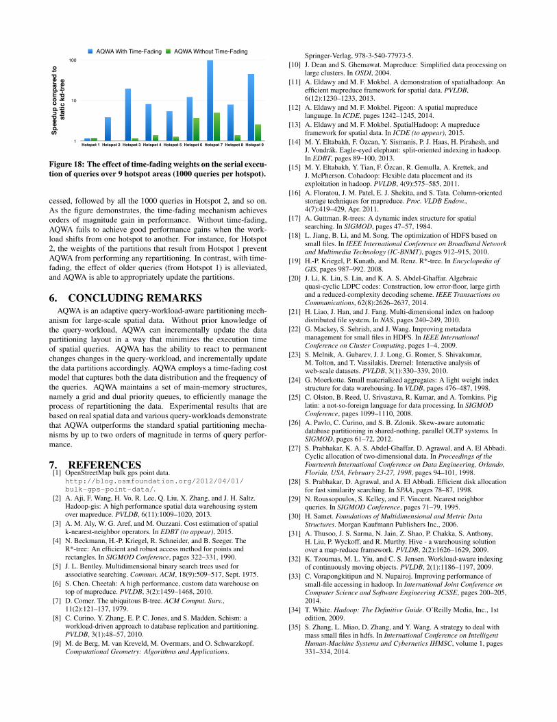
Table 1

Hotspot Static Index AQWA - No Archiving AQWA - With Archiving

Hotspot 1 7.281758808945E+126.05955656489E+12 6.145923441066E+12 1.20169829771647E+00 1.184811180740E+00

Hotspot 2 4.0728392064E+104.07083910185E+10 1.0468119712E+10 1.00049132488412E+00 3.8907075181E+00

Hotspot 3 2.2709691E+101.9296823088E+10 1.162396378E+09 1.17686164693723E+00 1.95369595344696E+01

Hotspot 4 6.3971465413E+104.5900609602E+10 7.891851193E+09 1.3936953336E+00 8.1060151602633E+00

Hotspot 5 4.6909550272E+103.6329262166E+10 8.65201464E+09 1.2912332229E+00 5.42180662237067E+00

Hotspot 6 1.44701390702E+113.9070188043E+10 1.1804809673E+10 3.70362667675784E+00 1.2257833434872E+01

Hotspot 7 4.0489734392E+108.101815728E+09 4.07324298E+08 4.99761235645818E+00 9.9404171542941E+01

Hotspot 8 7.3534957532E+105.327497592E+10 9.385507942E+09 1.38029076995592E+00 7.83494702539563E+00

Hotspot 9 3.2711398194E+101.259623537E+10 7.20873523E+08 2.59691862156749E+00 4.53774443786861E+01

10

Spee

dup

com

pare

d to

sta

tic k

d-tr

ee

1

10

100

Hotspot 1 Hotspot 2 Hotspot 3 Hotspot 4 Hotspot 5 Hotspot 6 Hotspot 7 Hotspot 8 Hotspot 9

AQWA With Time-Fading AQWA Without Time-Fading

Serial

�1

Figure 18: The effect of time-fading weights on the serial execu-tion of queries over 9 hotspot areas (1000 queries per hotspot).

cessed, followed by all the 1000 queries in Hotspot 2, and so on.As the figure demonstrates, the time-fading mechanism achievesorders of magnitude gain in performance. Without time-fading,AQWA fails to achieve good performance gains when the work-load shifts from one hotspot to another. For instance, for Hotspot2, the weights of the partitions that result from Hotspot 1 preventAQWA from performing any repartitioning. In contrast, with time-fading, the effect of older queries (from Hotspot 1) is alleviated,and AQWA is able to appropriately update the partitions.

6. CONCLUDING REMARKSAQWA is an adaptive query-workload-aware partitioning mech-

anism for large-scale spatial data. Without prior knowledge ofthe query-workload, AQWA can incrementally update the datapartitioning layout in a way that minimizes the execution timeof spatial queries. AQWA has the ability to react to permanentchanges changes in the query-workload, and incrementally updatethe data partitions accordingly. AQWA employs a time-fading costmodel that captures both the data distribution and the frequency ofthe queries. AQWA maintains a set of main-memory structures,namely a grid and dual priority queues, to efficiently manage theprocess of repartitioning the data. Experimental results that arebased on real spatial data and various query-workloads demonstratethat AQWA outperforms the standard spatial partitioning mecha-nisms by up to two orders of magnitude in terms of query perfor-mance.

7. REFERENCES[1] OpenStreetMap bulk gps point data.

http://blog.osmfoundation.org/2012/04/01/bulk-gps-point-data/.

[2] A. Aji, F. Wang, H. Vo, R. Lee, Q. Liu, X. Zhang, and J. H. Saltz.Hadoop-gis: A high performance spatial data warehousing systemover mapreduce. PVLDB, 6(11):1009–1020, 2013.

[3] A. M. Aly, W. G. Aref, and M. Ouzzani. Cost estimation of spatialk-nearest-neighbor operators. In EDBT (to appear), 2015.

[4] N. Beckmann, H.-P. Kriegel, R. Schneider, and B. Seeger. TheR*-tree: An efficient and robust access method for points andrectangles. In SIGMOD Conference, pages 322–331, 1990.

[5] J. L. Bentley. Multidimensional binary search trees used forassociative searching. Commun. ACM, 18(9):509–517, Sept. 1975.

[6] S. Chen. Cheetah: A high performance, custom data warehouse ontop of mapreduce. PVLDB, 3(2):1459–1468, 2010.

[7] D. Comer. The ubiquitous B-tree. ACM Comput. Surv.,11(2):121–137, 1979.

[8] C. Curino, Y. Zhang, E. P. C. Jones, and S. Madden. Schism: aworkload-driven approach to database replication and partitioning.PVLDB, 3(1):48–57, 2010.

[9] M. de Berg, M. van Kreveld, M. Overmars, and O. Schwarzkopf.Computational Geometry: Algorithms and Applications.

Springer-Verlag, 978-3-540-77973-5.[10] J. Dean and S. Ghemawat. Mapreduce: Simplified data processing on

large clusters. In OSDI, 2004.[11] A. Eldawy and M. F. Mokbel. A demonstration of spatialhadoop: An

efficient mapreduce framework for spatial data. PVLDB,6(12):1230–1233, 2013.

[12] A. Eldawy and M. F. Mokbel. Pigeon: A spatial mapreducelanguage. In ICDE, pages 1242–1245, 2014.

[13] A. Eldawy and M. F. Mokbel. SpatialHadoop: A mapreduceframework for spatial data. In ICDE (to appear), 2015.

[14] M. Y. Eltabakh, F. Ozcan, Y. Sismanis, P. J. Haas, H. Pirahesh, andJ. Vondrak. Eagle-eyed elephant: split-oriented indexing in hadoop.In EDBT, pages 89–100, 2013.

[15] M. Y. Eltabakh, Y. Tian, F. Ozcan, R. Gemulla, A. Krettek, andJ. McPherson. Cohadoop: Flexible data placement and itsexploitation in hadoop. PVLDB, 4(9):575–585, 2011.

[16] A. Floratou, J. M. Patel, E. J. Shekita, and S. Tata. Column-orientedstorage techniques for mapreduce. Proc. VLDB Endow.,4(7):419–429, Apr. 2011.

[17] A. Guttman. R-trees: A dynamic index structure for spatialsearching. In SIGMOD, pages 47–57, 1984.

[18] L. Jiang, B. Li, and M. Song. The optimization of HDFS based onsmall files. In IEEE International Conference on Broadband Networkand Multimedia Technology (IC-BNMT), pages 912–915, 2010.

[19] H.-P. Kriegel, P. Kunath, and M. Renz. R*-tree. In Encyclopedia ofGIS, pages 987–992. 2008.

[20] J. Li, K. Liu, S. Lin, and K. A. S. Abdel-Ghaffar. Algebraicquasi-cyclic LDPC codes: Construction, low error-floor, large girthand a reduced-complexity decoding scheme. IEEE Transactions onCommunications, 62(8):2626–2637, 2014.

[21] H. Liao, J. Han, and J. Fang. Multi-dimensional index on hadoopdistributed file system. In NAS, pages 240–249, 2010.

[22] G. Mackey, S. Sehrish, and J. Wang. Improving metadatamanagement for small files in HDFS. In IEEE InternationalConference on Cluster Computing, pages 1–4, 2009.

[23] S. Melnik, A. Gubarev, J. J. Long, G. Romer, S. Shivakumar,M. Tolton, and T. Vassilakis. Dremel: Interactive analysis ofweb-scale datasets. PVLDB, 3(1):330–339, 2010.

[24] G. Moerkotte. Small materialized aggregates: A light weight indexstructure for data warehousing. In VLDB, pages 476–487, 1998.

[25] C. Olston, B. Reed, U. Srivastava, R. Kumar, and A. Tomkins. Piglatin: a not-so-foreign language for data processing. In SIGMODConference, pages 1099–1110, 2008.

[26] A. Pavlo, C. Curino, and S. B. Zdonik. Skew-aware automaticdatabase partitioning in shared-nothing, parallel OLTP systems. InSIGMOD, pages 61–72, 2012.

[27] S. Prabhakar, K. A. S. Abdel-Ghaffar, D. Agrawal, and A. El Abbadi.Cyclic allocation of two-dimensional data. In Proceedings of theFourteenth International Conference on Data Engineering, Orlando,Florida, USA, February 23-27, 1998, pages 94–101, 1998.

[28] S. Prabhakar, D. Agrawal, and A. El Abbadi. Efficient disk allocationfor fast similarity searching. In SPAA, pages 78–87, 1998.

[29] N. Roussopoulos, S. Kelley, and F. Vincent. Nearest neighborqueries. In SIGMOD Conference, pages 71–79, 1995.

[30] H. Samet. Foundations of Multidimensional and Metric DataStructures. Morgan Kaufmann Publishers Inc., 2006.

[31] A. Thusoo, J. S. Sarma, N. Jain, Z. Shao, P. Chakka, S. Anthony,H. Liu, P. Wyckoff, and R. Murthy. Hive - a warehousing solutionover a map-reduce framework. PVLDB, 2(2):1626–1629, 2009.

[32] K. Tzoumas, M. L. Yiu, and C. S. Jensen. Workload-aware indexingof continuously moving objects. PVLDB, 2(1):1186–1197, 2009.

[33] C. Vorapongkitipun and N. Nupairoj. Improving performance ofsmall-file accessing in hadoop. In International Joint Conference onComputer Science and Software Engineering JCSSE, pages 200–205,2014.

[34] T. White. Hadoop: The Definitive Guide. O’Reilly Media, Inc., 1stedition, 2009.

[35] S. Zhang, L. Miao, D. Zhang, and Y. Wang. A strategy to deal withmass small files in hdfs. In International Conference on IntelligentHuman-Machine Systems and Cybernetics IHMSC, volume 1, pages331–334, 2014.