Arbitrage activity and price discovery acrossspot, futures and ETF markets

Qingfu Liu∗, Zhongyuan Gao†, and Michael T. Chng‡

Current draft: 23rd May 2015

Abstract

We examine how the introduction of exchange-traded fund (ETF) affects the arbi-trage and price discovery mechanism between the China Securities Index (CSI)300 spotand futures markets. Utilizing a bivariate Smooth-Transition VECM (ST-VECM), weaccommodate a two-speed error-correction mechanism to differentiate price discoverybetween no-arbitrage versus arbitrage states. Our analysis yields three main findings:i) Post-ETF trading, we see a substantial reduction in observed pricing errors. This isexpected given a narrower no-arbitrage band due to lower transaction cost from tradingETF; ii) The futures market still contributes more price discovery than its spot indexand ETF counterparts; iii) Arbitragers migrated from the CSI300 spot predominatelyto the ETF traded in Shanghai, seemingly ignoring the ETF traded in Shenzhen. Whenarbitragers are present, the Gonzalo and Granger (GG 1995) price discovery measure isnoisy since the VECM averages the error-correction mechanism between no-arbitrageand arbitrage states. A modified GG measure from the ST-VECM addresses this issue.We explain why the price discovery bound that corresponds to the no-arbitrage state,provides a clearer indication of cross-market price discovery contribution.

JEL classification: G14, G15.

Keywords: Cost of carry; arbitrage; price discovery, index futures.

∗School of Economics, Fudan University, China.†Information Management Analytic, HSBC China.‡Corresponding author’s email: Michael.Chng@xjtlu.edu.cn. International Business School Suzhou

(IBSS), Xian-Jiaotong Liverpool University, and Department of Finance, Deakin University. We thank par-ticipants at the Institute for Quantitative Finance Workshop, Peking University HSBC Business SchoolShenzhen, and Deakin University. Liu acknowledges funding support from the National Nature ScienceFunds of China (Grant 71473042).

1

1 Introduction

In April 2010, the China Financial Futures Exchange (CFFEX) launched the China Securities

Index 300 (CSI300) futures contract. During its first three months of trading, average daily

turnover volume reached RMB 230.8 billion (USD 40 billion), which exceeds the aggregate

turnover volume of its constituent firms. In just its first year, CSI300 futures average trading

volume has exceeded the KOSPI, Hang Seng and TAIEX futures markets. Compared to 2010,

turnover volume increased by around 33% during the first half of 2012. More astoundingly,

the second half of 2012 saw a further 60% increase in turnover volume over the first half. In

less than three years after its launch, the CSI300 futures contract has grown to become one

of the world’s most actively traded equity index derivative. According to the 2013 survey by

the Futures Industry Association, the CSI300 futures is ranked tenth globally among equity

index derivative markets in terms of (contracts) trading volume. In May 2012, two fund

management companies, Huatai-Pinebridge and Jiashi-Harvest, correspondingly launched

CSI300 exchange traded funds (ETFs) on the Shanghai and Shenzhen stock exchange.

Our motivation is to acquire a better understanding of the arbitrage and price discovery

mechanism among the CSI300 spot, futures and ETF markets. In developed countries, the

introduction of ETF trading implies a straightforward migration by arbitragers from a non-

tradable index to a tradable close-substitute. But in China, it is complicated. The CSI300

is designed to gauge the overall performance of the country’s A-share market across both

stock exchanges. The concurrent introduction of ETF trading on both exchanges raises an

interesting question as to how arbitragers respond. Ex-ante, without limits to arbitrage,

arbitragers will distribute themselves to equate the marginal net profit on both ETFs to zero.

But if arbitragers persistently cluster on one ETF despite non-trivial carry-cost violation on

the other ETF, this necessarily imply limits to arbitrage that somehow bind only one of the

two exchanges e.g. trading rule, short-sale constraint, settlement procedure, liquidity etc.

Prior studies show that futures market leads the spot market in price discovery based

on both U.S. [Kawaller et al. (1987), Edwards (1988), Stoll and Whaley (1990), Chan et al.

(1991), Chan (1992), Hasbrouck (1995), Fleming et al. (1996)] and international evidence

2

[Ryoo and Smith (2004), Zhong et al. (2004) and Bose (2007)] for South Korean, Mexi-

can and Indian markets respectively]. The greater price discovery contribution is commonly

attributed to greater liquidity, more sophisticated investors [Chu et al. (1999)] and/or non-

trading in constituent stocks [Miller et al. (1994)], which ‘drags’ the spot index price from

adjusting to new information. However, these explanations do not readily apply to ETFs.

Booth et al. (1999) analyze price discovery across the German DAX index, futures and

options markets. The authors find that the option market actually contributes less price

discovery than the spot index, which they attribute to higher transaction cost in option

markets. So and Tse (2004) find that Hang Seng futures contributes the most price discovery.

But surprisingly, the Hang Seng tracker fund provides less price discovery than the spot

index. Hasbrouck (2003) finds that most of the price discovery for the S&P500 and Nasdaq100

comes from the E-mini futures market. But for the S&P400 Midcap, price discovery is shared

between the futures and ETF.

Spot-futures arbitrage violation is extensively studied for developed markets, including

Yadav and Pope (1990) for the FTSE 100, Lim (1990) and Brenner et al. (1989) for the

Nikkei 225. MacKinlay and Ramaswamy (1988) is one of the first papers to distinguish up-

per and versus lower arbitrage bound intra-day violations between the S&P500 spot and

futures, which they associate with dissimilar transaction cost. Miller et al. (1994) attribute

mean-reversion in the S&P500 basis to infrequent trading in constituent stocks, rather than

arbitrage trading. Brennan and Schwartz (1990) highlight that the position limit of arbi-

tragers provide a better understanding of fluctuations in the basis.

We have two related objectives. First, we utilize a bivariate Smooth Transition Vector

Error-Correction Model (ST-VECM) to estimate non-linear return dynamics for four sepa-

rate pairwise market analysis of the CSI300 futures against: i)+ii) CSI300 spot rft ∼ rst in

the pre- and post-ETF sample period, iii) Huatai-Pinebridge ETF (or SHETF) traded in

Shanghai rft ∼ rSHt, and iv) Jiashi-Harvest ETF (or SZETF) traded in Shenzhen rft ∼ rSZt.

We specify the error-correction variable in the ST-VECM as the carry-cost adjusted basis bt.

The ST-VECM allows the VECM’s error-correction mechanism to take on a ‘second-gear’

in response to arbitrage activity. It is reasonable to assume that any adjustment in bt will

3

differ depending on whether bt is fluctuating within or outside its no-arbitrage band. This

implies that a VECM specification is sub-optimal.

The ST-VECM also has merit over regime-switching models that impose discrete tran-

sition processes. Such models assume an abrupt switch in the error-correction mechanism,

which may be suitable for a matured market populated by savvy arbitragers ready to pounce

at any mispricing opportunities. However, both CSI300 ETFs, and even the futures contract,

were introduced less than six years ago. Furthermore, trading is dominated by individual

investors1. Even if arbitragers are present, any mispricing adjustment back within the no-

arbitrage band is likely to be gradual rather than abrupt, To address this issue, we specify

a smooth transition function for the error-correction mechanism. Taylor et al. (2000) apply

the ST-VECM to compare FTSE 100 spot and futures mispricing adjustments before and

after electronic trading. Delatte et al. (2012) estimate information transmission between the

sovereign CDS and bond markets for Euro-zone countries using an ST-VECM.

Our second objective is to apply the ST-VECM to compute a modified Gonzalo and

Granger (1995) or GG measure of price discovery contribution for each of the four pairwise

market estimations. If arbitrage trading generates a two-speed error-correction mechanism,

this necessarily implies that the original GG (1995) measure is noisy. The VECM does not

accommodate the impact of arbitrage activity on the error-correction mechanism between

the two markets. Intuitively, when bt−d becomes profitably non-trivial, arbitrage trading will

force spot and futures prices towards each other. This causes the error-correction coefficients

(λs, λf ) to register a more comparable price impact between rst and rft. But since arbitrage

trading does not occur all the time, the VECM’s estimated (λs, λf ) reflect an ‘average’

error-correction mechanism between arbitrage and no-arbitrage states. Consequently, the

GG (1995) measure, which is based on (λs, λf ), is a noisy measure that encapsulates the

price impact of both informed traders as well as arbitragers.

We show how a modified GG measure from the ST-VECM addresses the preceding issue.

The modified measure consists of a pair of price discovery upper GG0 and lower bound GG1

1According to CFFEX market reports, individual investors constitute more than 80% of average dailytrading volume.

4

that correspond to the no-arbitrage and arbitrage states. Hence, the Gap between GG0 and

GG1 indicates the extent of arbitrage activity between two markets. Comparisons in Gap over

time and/or across pairwise markets provide insights into the migration of arbitrager post

ETF introduction. If arbitrage activity is weak or non-existent, this implies an insignificant

two-speed error-correction, and consequently a trivial distinction between GG0 and GG1.

Put simply, the ST-VECM reduces to a VECM.

In the pre-ETF sample, we document a significant two-speed error-correction mechanism

in both spot rst and futures rft return equations. The second-gear adjustment is delivered

through bt−dF [bt−d, γ], where 0 ≤ F [bt−d, γ] ≤ 1 is the transition function, γ is the transition

speed coefficient, and bt−d is the error-correction variable. Our result indicates the presence

of arbitragers, whose trading activity in response to a non-trivial bt−d affects both rst and rft.

The joint price impact exerted by bt−d is larger on rst than rft, which as expected, indicates

that the futures market contributes more price discovery than the spot index. The average

F [bt−d, γ] value, or FAvg is 0.262, and γ = 0.31 is significant at the 1% level.

In the post-ETF sample, the two-speed error-correction mechanism remains significant in

rst, but not in rft. As such, only the spot price responds to a non-trivial bt−d. This suggests

that, post-ETF, arbitrage trading between the CSI300 spot and futures markets has either

ceased, or it is substantially reduced. The joint price impact of bt−d on rst is now even larger

than on rft, compared to the pre-ETF sample. FAvg = 0.636 with γ = 1.466 that is significant

at the 10% level.

It is in the SHETF and futures estimation that we find a significant two-speed error-

correction mechanism in both rSHt and rft. The joint price impact exerted by bt−d remains

larger on rSHt than rft, but the difference is comparable to the pre-ETF sample. Further-

more, while FAvg = 0.633 is comparable to the post-ETF rst ∼ rft estimation, its speed

of adjustment coefficient γ = 2.594 is larger and significant at the 1% level. A comparable

FAvg but a larger, more significant γ indicates that smaller pricing errors occur between

the SHETF and futures markets. This is expected given a narrower no-arbitrage band for

rSHt ∼ rft compared to rst ∼ rft, due to lower transaction costs from trading an ETF com-

pared to constituent stocks. The results also suggest that index arbitrager migrated from the

5

CSI300 spot to the SHETF, such that mispricing in bt−d are traded away more rapidly. This

is consistent with our finding that the significant two-speed error correction mechanism in

the pre-ETF sample is found in rSHt ∼ rft, but not in rst ∼ rft, post-ETF.

In stark contrast, the rSZt ∼ rft estimation reveals that neither rSZt nor rft exhibit a two-

speed error correction mechanism. More surprisingly, there is no significant error-correction

mechanism in the SZETF and futures cross-market return dynamics. Out of the four pairwise

market estimation, rSZt ∼ rft yield the largest FAvg = 0.907, which is near its maximum.

To follow, its γ = 1.174 is the only speed of adjustment coefficient that is insignificant.

These results strongly suggest that, after both CSI300 ETFs were simultaneously launched,

index arbitragers migrated predominately to the SHETF traded in Shanghai, and seemingly

ignored the ETF traded in Shenzhen.

Our paper proceeds as follow. The next section contains sample description and institu-

tional background. The ST-VECM is outlined in section 3, and empirical results are reported

in section 4. Section 5 concludes.

2 Institutional background

2.1 The CSI300 spot, futures and ETF markets

Driven by over 15 years of economic expansion, China’s financial markets are receiving

increasing attention from both the investment and academic communities. The two main

stock exchanges, located in Shanghai and Shenzhen, were established in 1990 and 1991

respectively. From inception, both stock exchanges maintain their own broad-based market

indices, namely, the Shanghai Composite Index and the Shenzhen Composite Index. On 8-

April-2005, the China Securities Index (CSI) Company Ltd launched the CSI300 with the

aim to provide a comprehensive indicator of the A-share market’s overall performance across

the two stock exchanges. The index comprises 300 of the largest and most actively traded

A-shares that are listed in either Shanghai or Shenzhen, and represents around 70% of total

6

market capitalization of both stock exchanges2.

Five years after the CSI300 was introduced, CFFEX launched the CSI300 futures in April

2010. We outline key contractual specifications in Table 1. Each CSI300 futures contract has

a RMB300 contract multiplier, and is governed by a tick size of 0.2 index point, or RMB60.

The contract expires on the third Friday of the delivery month. There are four available

delivery months: current month, next month, and the next two quarter-months i.e. final

months of the next two quarters3. As with many other futures markets around the world,

CSI300 futures trading volume is concentrated on the front contract, which accounts for

more than 95% of aggregate trading volume. On average, three days before expiry, traders

roll-over from the current to the next delivery month. Accordingly, our time-series data is

constructed using the front contract. On the third Tuesday of every month, we switch over

from the current to the next contract month. This allows us to construct a continuous time

series of futures data over the relevant sample periods.

INSERT TABLE 1

Since it is a relatively new market, the CSI300 futures contract is closely regulated. To

open a margin account, an individual investor is required pass a compulsory qualifications

exam, and deposit a minimum RMB 0.5 million (m) into a trading account4. The RMB

0.5m deposit is non-trivial given that domestic institutional investors are only required to

deposit RMB 1m5. Qualified Foreign Institutional Investors (QFII) are not allow to trade

CSI300 futures. The CFFEX clearing house imposes a 15% (18%) initial margin for the

current and next month (next two quarter month) contracts6. From 29-June-2012, the margin

2The CSI300 base value is set to 1000 on 31-Dec-2004. Every six months, firms are sorted by marketcapitalization and turnover volume, and the index is updated for new constituent firms. The value of theindex is computed every second and published every 5 seconds.

3For example, if we are in early January, the delivery months are January, February, March and June. Ifwe are in March, the delivery months are March, April, June and September, and so forth.

4To note, this is not a margin requirement, since the trading account needs to be established beforeundertaking any futures trading.

5It is explicitly mentioned in various regulatory documents issued by the China Securities RegulatoryCommission that index futures is not suited for individual investors.

6Margin accounts can only be maintained with cash. Other liquid assets, such as stocks and bonds, arenot recognized as collateral for satisfying margin requirements.

7

requirement is adjusted to 12% for all four contract cycles. The balance in the margin account

earns a risk-free rate that is based on the Shanghai Interbank Offer Rate (SHIBOR)7.

The first two CSI300 ETFs were launched in China on 28-May-2012. The Huatai-PineBridge

ETF (Stock Code 510300), or SHETF, is listed on the Shanghai Stock Exchange, while the

Jiashi-Harvest ETF (Stock Code 159919), or SZETF, is launched on the Shenzhen Stock Ex-

change. Our analysis is based on synchronized one-minute observations over a three months

pre-ETF and post-ETF sample. The pre-ETF sample period runs from 27-February to 28-

May 2012, and covers both CSI300 spot and futures market. The post-ETF sample period

runs from 01-December-2012 to 28-February-2013, and covers data for all four CSI300 mar-

kets. We skip the first six months after ETF launch to avoid any trading anomalies associated

a newly introduced market from contaminating our results8.

Both stock exchanges trade four hours a day between 09:30 to 11:30, and from 13:00

to 15:00. The CSI300 futures market opens 15 minutes earlier and closes 15 minutes later

than the stock markets, but shares the same lunch-break from 11:30 to 13:00. Our analysis

is based on overlapping trading hours across the four CSI300 markets, which gives a total

of 240 one-minute observations per trading day for around 65 trading days in each of the

pre-ETF and post-ETF samples.

CSI300 constituent firms pay dividends throughout the year. However, dividend pay-

outs are clustered mainly during the high earnings reporting season from May to September.

In 2013, we compute the monthly annualized dividend yield, and find that it ranges from

1.21%pa in May to 2.3%pa in September. For other months, the dividend yield is around

0.8%pa for 2013, and even lower for 2012. Indeed, firms in China typically pay much lower

dividends compared to similar firms in Western economies. Furthermore, since both pre- and

post-ETF sample periods are from the low earnings reporting season, we assume q = 0%9.

Our main focus is on the comparison among the four pairwise market estimations. The level

7In our analysis, we also use the 3-month Treasury yield and the RMB prime rate. Both rates are verysimilar to SHIBOR, and so are our main results.

8Furthermore, during the first six months, the data format and structure for the SZETF is different fromthe other three CSI300 markets.

9We can confirm that the dynamics of bt over time is unaffected by whether we use q = 0 or 0.8%pa.

8

of q cannot explain dissimilar findings across the various pairwise estimations.

2.2 Prior studies on derivative markets in China

The majority of studies on derivative markets in China examine industrial commodity futures

of the Shanghai Futures Exchange (SHFE) and/or agricultural futures traded either the

Dalian or Zhengzhou Futures Exchange. Fung et al. (2010) study the information flow in

copper and aluminum futures markets between China and U.S., while Fung et al. (2003)

conducts a similar study that focuses on agricultural commodity futures. Liu and An (2011)

analyze cross-market price discovery between U.S. and China for the copper and soybean

futures markets. Hua and Chen (2007) examines information flow in industrial metal futures

traded between SHFE and the London Metal Exchange, as well as agricultural futures traded

between Dalian Exchange and CBOT. Lee et al. (2009) compares day-of-the-week effects

between U.S. and Chinese commodity futures. Chan et al. (2004) analyze the determinants

of daily volatility behavior in the soybean contract in Dalian, and the mungbean and wheat

contracts traded in Zhenzhou.

The introduction of the CSI300 futures contract in 2010 opened up new avenues of deriva-

tive research on China’s first stock index futures market. Yang et al. (2012) find that price

discovery in the newly launched contract did not function well, which they attribute to high

barriers to entry for informed foreign investors. Chen et al. (2012) report that stock market

volatility has decreased significantly after the introduction of CSI300 futures trading. Zhuo

et al. (2012) analyze arbitrage violation and mean-reversion in the CSI300 futures market

over a six months period. Their mean-reverting model contains dummy variables to indi-

cate arbitrage violation. However, this imposes a rapid shift in the mean-reverting process

when an arbitrage violation occurs. This assumes that the supply of arbitrage activity is

highly elastic, which is not appropriate for a newly launched market dominated by poorly

capitalized individual investors.

9

3 ST-VECM estimation and modified GG measure

In equation (1), an arbitrage violation occurs when the carry-cost adjusted basis bt exceeds

either its lower TCL or upper TCU arbitrage bound. These bounds normally reflect the

applicable round-trip transaction cost associated with index arbitrage. Denote St and Ft as

spot and futures prices, r and q respectively as the continuously compounded annualized risk-

free rate and dividend yield on the CSI300 index. In equilibrium, the pricing error bt ∼ (0, σb)

fluctuates within its bounds over the life of the contract T − t. Setting TCU 6= TCL allows

for dissimilar transaction cost associated with short and long arbitrage10.

bt = Ft − Ste(r−q)(T−t)

TCU ≥ bt ≥ −TCL,where TCU 6= TCL (1)

The widely used Gonzalo-Granger (1995) (GG) common-factor weights measure of cross-

market price discovery is based on a VECM specification. Since the VECM assumes a linear

error-correction mechanism, the GG measure imposes a single-speed adjustment by bt, re-

gardless of whether bt triggers an arbitrage violation. Intuitively, we expect bt to deliver more

price impact on both rst and rft equations when arbitrage trading is taking place between

the two markets. This implies that a non-linear error-correction mechanism, which facilitates

a two-speed adjustment, is a more appropriate empirical specification. Furthermore, since

trading in CSI300 markets is dominated by smaller retail investors, the adjustment by bt back

within its arbitrage-free bounds is likely to occur gradually over time. As such, a discrete

regime-switching model would not be appropriate.

We elaborate on how the ST-VECM in equation (2) addresses the above concerns.

Bounded between [0,1], the transition function F [bt−d, γ] is determined by the speed of ad-

justment parameter γ, the magnitude of bt−d and its variability σbt−d . Since our analysis

10When bt > TCU , this triggers short arbitrage i.e. short-futures, long-spot, and reversing later on. Whenbt < −TCL, this triggers long arbitrage i.e. going long-futures and short-spot. Normally, we expect TCU <TCL, since it is more expensive to go short rather than long in the underlying index.

10

covers newly launched CSI300 ETF markets, we allow illiquidity variables ILLQst = rstSizest

and ILLQft =rft

Sizeftfrom both markets to enter the ST-VECM as exogenous variables.

Chakravarty et al. (2004) find that liquidity help explains lead-lag effects. We construct the

illiquidity variables as price impact conditional on trade size, in the spirit of Amihud (2002).

rft = αf0 +T∑i=1

(αs1irst−i + αf1irft−i + [βf0 + βs1irst−i + βf1irft−i] · F [bt−d, γ])

+ (λf1 + λf2 · F [bt−d, γ])bt−d + δs1ILLQst−1 + δf1 ILLQft−1 + εft

rst = αs0 +T∑i=1

(αs2irst−i + αf2irft−i) + [βs0 + βs2irst−i + βf2irft−i] · F [bt−d, γ])

+ (λs1 + λs2 · F [bt−d, γ])bt−d + δs2ILLQst−1 + δf2 ILLQft−1 + εst

F [bt−d, γ] = 1− exp−γ(bt−dσt−d

)2 ∈ [0, 1] (2)

Consider when there is no significant two-speed error-correction, such that γ = 0. This

implies F [bt−d, γ] = 0, and the ST-VECM reduces to a VECM. Conversely, if a non-linear

error-correction mechanism is inherent in the data i.e. γ > 0, a statistically non-trivial

pricing error bt−dσbt−d

will cause F [bt−d, γ] to increase. When this happens, a second set of error-

correction coefficients (λs2, λf2) is introduced into the VECM. Accordingly, the F [bt−d, γ] in

the ST-VECM allows the error-correction mechanism between two markets to shift between

first-gear (λs1, λf1) and second-gear (λs1 + λs2, λ

f1 + λf2) in response to a non-trivial bt−d.

Just as the GG (1995) measure is based on the VECM’s error-correction coefficients

(ECC), the modified measure GGt in equation (3) is calculated from the ECCst and ECCf

t

of the ST-VECM. Functional forms aside, the intuitive interpretation of the original GG

(1995) measure flows directly onto the modified version. Specifically, the magnitude of the

ECCs indicate each market’s reliance on the error-correction variable for their price formation

over time. If ECCst > ECCf

t , this implies that rst is affected more by deviations between

St and Ft, compared to rft. The modified GGt is based on the spot market. Hence, a larger

11

(smaller) GGt implies that the spot market performs less (more) price discovery, relative to

the futures market.

ECCst = λs1 + λs2F [bt−d, γ] ECCf

t = λf1 + λf2F [bt−d, γ]

GGt =ECCs

t

ECCst − ECC

ft

(3)

The transition function F [bt−d, γ] induces fluctuation in ECCst between λs1 and (λs1 +λs2),

and in ECCft between λf1 and (λf1 + λf2). As such, equation (4) shows that GGt is bounded

between GG0 when F [bt−d, γ] = 0, and GG1 when F [bt−d, γ] = 1. Whether GG0 (or GG1) is

the upper or lower bound depends on the estimated λs. It is easy to show11 that ifλs1λs2<

λf1λf2

,

then GG0 and GG1 are the upper and lower bounds respectively, and vice versa.

GG0 =λs1

λs1 − λf1

GG1 =λs1 + λs2

(λs1 + λs2)− (λf1 + λf2)

GG0 > GG1 ifλs1λs2

<λf1

λf2GG1 > GG0 if

λs1λs2

>λf1

λf2(4)

The original GG (1995) measure, which has the same functional form as GG0, is bounded

between 0 and 1. This is because the estimated λs and λf from the VECM have opposite

signs, such that 0.5 is the threshold value to determine which market possesses the price

leadership role i.e. contributes more price discovery. Equation (4) shows that this is not the

case for GGt, since λs1 and λf1 can have the same sign. Furthermore, the values of GG0 and

GG1 can differ across pairwise markets, since the estimated {λs1, λs2, λf1 , λ

f2} are likely to be

different.

11The condition GG0 > GG1 corresponds to λs1(λs1 +λs2−λf1 −λ

f2 ) > λs1(λs1 +λs2−λ

f1 )−λf1λs2, or

λs1

λs2<

λf1

λf2

12

4 Discussion of empirical results

4.1 Basic features of the sample and diagnostic test

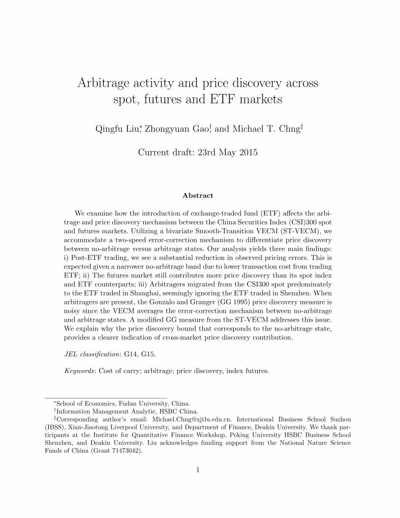
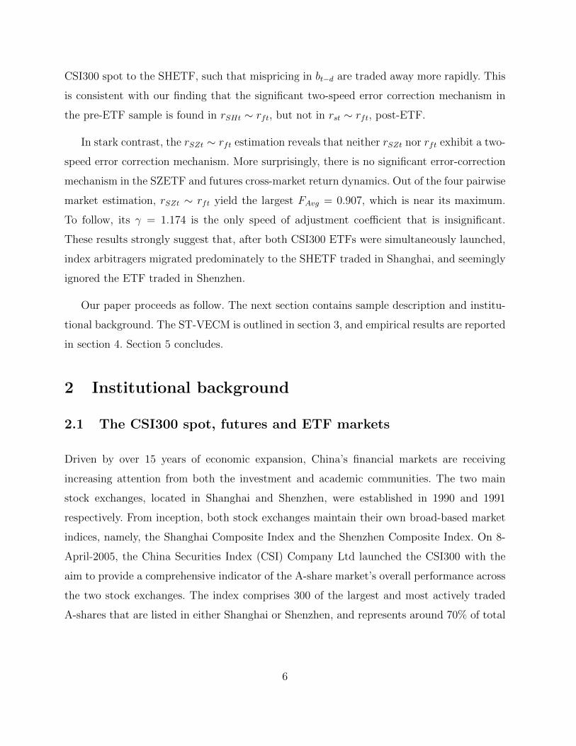
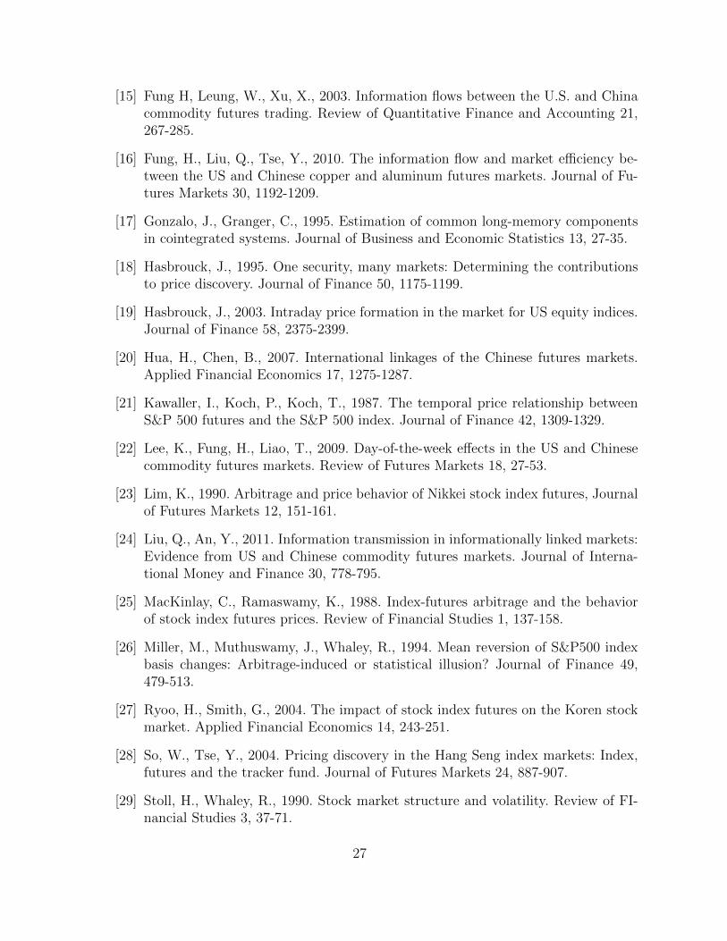
We present preliminary results to reveal some basic features of the sample. Figures 1A∼D

plot the price series for each of the four pairwise market estimations. Given that they are

all closely-related securities, it is not surprising to observe evident price co-movements over

time. However, we notice that in Figure 1D, SZETF and futures prices seems to exhibit

greater discrepancy over time compared to its two spot market counterparts in Figures 1B

and 1C.

INSERT FIGURE 1

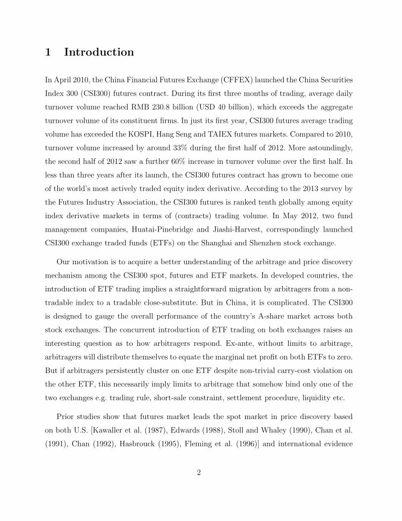
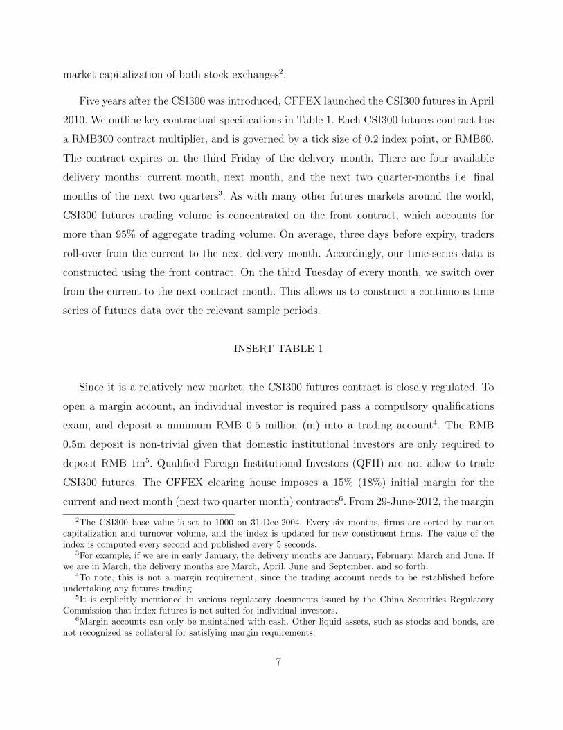
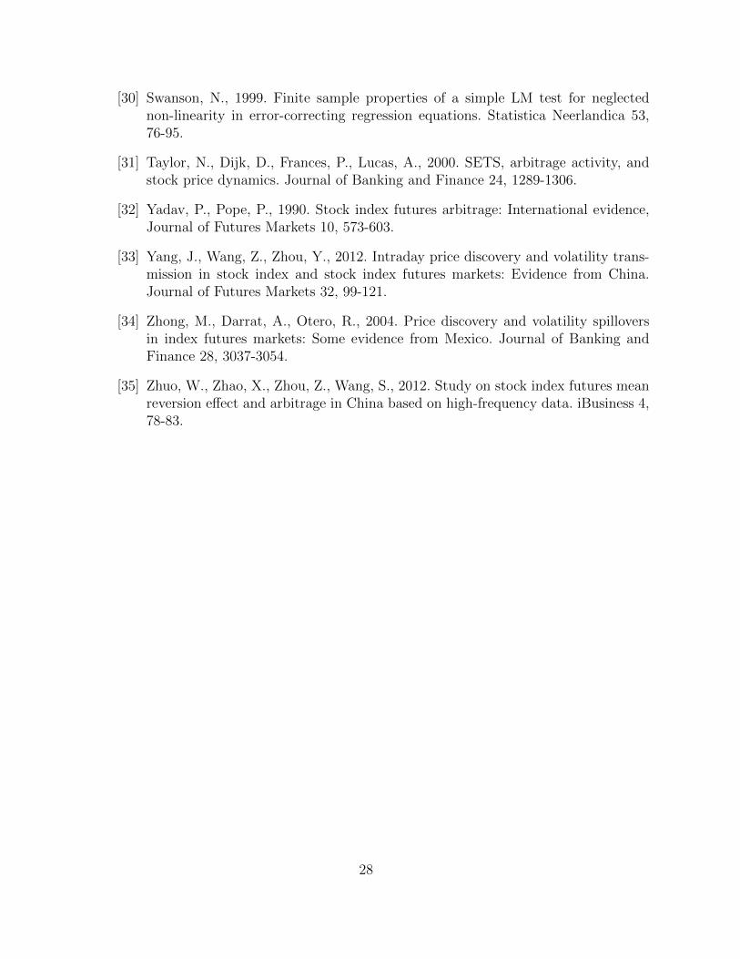
Next, we compare the return series of the four pairwise markets in Figures 2A∼D. For the

post-ETF sample, rft is the same across Figures 2B∼D. Using rft as a visual benchmark, we

can see that the relevant spot market return becomes increasing volatile as we move from rst

in Figure 2B to rSHt in Figure 2C, and again to rSZt in Figure 2D. Based on the descriptive

statistics12, we can confirm that: rst is less volatile than rft; rSHt has comparable volatility

to rft; rSZt is more volatile than rft.

INSERT FIGURE 2

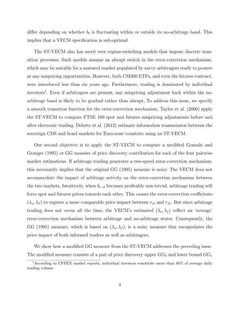
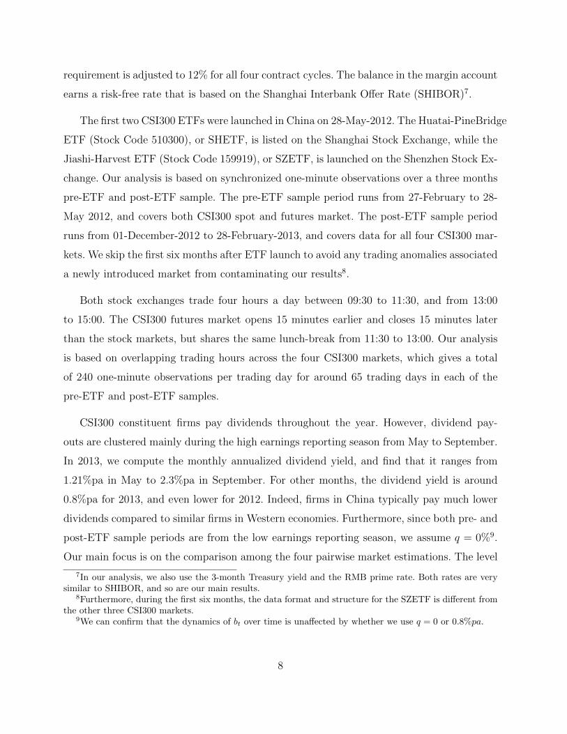
To follow, we plot the carry-cost adjusted basis bt corresponding to the four pairwise

markets in Figures 3A∼D. Consistent with the two previous figures, Figure 3 shows that the

bt between the SZETF and futures market exhibits the largest mean and volatility compared

to the other two pairwise markets. These visual plots provide some early indication that the

trading link between SZETF and the futures market seems to be weaker compared to either

the SHETF or the spot index.

INSERT FIGURE 312The descriptive statistics on the key variables pre- and post-ETF are not included due to space constraint.

They are readily available upon request.

13

Lastly, we conduct Augmented Dickey-Fuller (ADF) tests to confirm the stationarity

of the key variables that are used in the ST-VECM13. We use the Schwarz Information

Criterion to determine the optimal lag specification for the ADF test on each variable. At

the 1% significance level, we can confirm that all the price series are non-stationary, but the

log difference in prices are all stationary. Furthermore, bt−d and the illiquidity variables for

all four pairwise markets are stationary as well.

4.2 Estimation results from the ST-VECM

The ST-VECM estimation requires a lag specification for the spot and futures return dy-

namics, as well as the error-correction variable bt−d. An analysis of the auto- and cross-auto

correlation functions indicate that all return series exhibit lag-1 dynamics. However, bt−d is

the key variable in the ST-VECM that affects both the transition function F [bt−d, γ], and the

relative movements in spot and futures prices over time. Furthermore, since the estimation is

conducted using 1-minute observations, the error-correction mechanism inherent in the data

may be occurring at longer lags i.e. d > 1. Hence, we conduct a formal test to determine an

optimal d for bt−d, which is then apply to all four pairwise market estimations.

Swanson (1999) proposes a Lagrange-Multiplier (LM) test for non-linear error-correction

mechanism, which the ST-VECM is intended to capture. Following Swanson (1999), we

perform a third-order Taylor-Series expansion on each return series around bt−d, and test for

the joint significance of higher-order terms. Equation (5) outlines the LM test on rft. If the

higher-order terms are jointly insignificant i.e. H0 : φ1 = φ2 = φ3 = 0, then we fail to reject

the null hypothesis of no significant non-linear dynamics in rft. The LM-test is repeated for

d = 1, 2, ... to ascertain the optimal d for which most of not all of the return series exhibit

non-linear dynamics. Intuitively, the LM-test allows us to determine an optimal d that allows

the ST-VECM to bring out non-linear interactions in return dynamics between markets.

13Due to space constraint, and since these are standard results, we do not report them in the paper. TheADF test statistics are readily available upon request.

14

rft =φ0(ft−1 + st−1 + bt−d)

+φ1(ft−1 + st−1 + bt−d)bt−d + φ2(ft−1 + st−1 + bt−d)b2t−d + φ3(ft−1 + st−1 + bt−d)b

3t−d (5)

We report the LM-test statistics in Table 2 for d = 1, 2..., 5. For the pre-ETF sample,

rft exhibits non-linear dynamics up to bt−3, whereas rst displays non-linear dynamics up to

bt−5. These results are also documented in the post-ETS sample. In contrast, both rSHt and

rSZt exhibit non-linear effect only for d = 4, for which there is no significance for rft. Since

the futures market is involved in all four pairwise estimation, we do not consider d = 4. In

addition, among d = 1, 2, 3, the test statistics for the various markets are the highest for

d = 3. Hence we specify d = 3 for bt−d and F [bt−d, γ] in the ST-VECM estimation.

INSERT TABLE 2

We present the estimation results in Table 3 Panels A and B for the pre- and post-ETF

sample. In Panel A, rst−1 · F [bt−d, γ] and rft−1 · F [bt−d, γ] are significant in both rft and

rst equations. This indicates substantial non-linear own- and cross-market return dynamics

between the spot and futures markets, even after controlling for illiquidity effects across both

markets. There is also an evident two-speed error-correction mechanism, with bt−d ·F [bt−d, γ]

significant in both rft and rst equations. For the error-correction coefficients, we find that

|λs1| > |λf1 | and |λs1 + λs2| > |λ

f1 + λf2 |. This indicates that bt−d exerts a larger price impact

on rst compared to rft. The estimated λs imply that the modified GG measure assigns the

price leadership role to the futures market. For F [bt−d, γ], the speed of adjustment coefficient

γ = 0.31 is also significant at the 1% level. In sum, these results indicate the presence of

arbitrage activity between the CSI300 spot and futures market in the pre-ETF sample.

INSERT TABLE 3

In the post-ETF sample, the rst ∼ rft estimation results in Panel B are generally con-

sistent with Panel A, but with two exceptions. The two-speed error-correction mechanism

15

is no longer significant in rft, although it remains significant in rst. Interestingly, γ = 1.466

indicates a faster speed of adjustment in bt−d compared to pre-ETF γ, albeit less significant

at the 10% level.

The rSHt ∼ rft estimation reveals significant cross-market non-linear return interactions,

with rft−1 ·F [bt−d, γ] and rSHt−1 ·F [bt−d, γ] correspondingly significant in rSHt and rft. How-

ever, own-market non-linear return dynamics are insignificant. A two-speed error-correction

mechanism is significant in both rSHt and rft, with the estimated coefficients also having

larger magnitudes in the rSHt equation. Lastly, the speed of adjustment γ = 2.594 is larger

and highly significant, compared to the rst ∼ rft estimation.

Lastly, the rSZt ∼ rft estimation reveals starkly dissimilar findings. Only rSZt−1 ·F [bt−d, γ]

is significant in rft. There are no significant two-gear error-correction mechanisms in either

rSZt or rft, although, consistent with the other three pairwise estimations, the magnitude of

error-correction coefficients are larger for rSZt compared to rft. More surprisingly, even bt−d is

insignificant in both equations. The speed of adjustment g = 1.174 is also insignificant. One

could associate these findings to the diagnostic results in Table 2, which indicate that rSZt

does not exhibit non-linear effects at bt−3. However, this is also the case for rSHt. Hence, a

potentially sub-optimal lag specification for bt−d cannot explain the dissimilar results between

rSZt and rSHt.

4.3 Price discovery over time

4.3.1 Price impact and error-correction mechanism

To facilitate a more comprehensive discussion of findings across the four pairwise market

estimations, we provide a summary of key results in Table 4. Our focus is on ST-VECM

estimates that provide insights into the impact of ETF trading on price discovery across

CSI300 markets. In Table 3, the ST-VECM consistently yields |λs1| > |λf1 | and |λs1 + λs2| >

|λf1 +λf2 | across all four pairwise market estimations. This strongly indicates that the CSI300

futures market contributes more price discovery than its three spot market counterparts.

In Table 4, we report the joint price impact of lag-1 returns and bt−3 on the correspond-

16

ing markets of each pairwise estimation. This includes the second-gear price impact that is

delivered through F [bt−d, γ] on the estimated coefficients for each variable. However, since

F [bt−d, γ] varies over time, we compute the associated price impact based on the average

F [bt−d, γ], or FAvg, over the sample period, corresponding to each pairwise market. For ex-

ample, consider the rSHt ∼ rft estimation. In the rSHt equation, the joint price imposed by

bt−d is [λsh1 + λsh2 · FAvg]. This corresponds to 0.046 in the last column of Table 4, where

(**/**) indicates that both λsh1 and λsh2 are significant at the 5% level.

INSERT TABLE 4

The pre-ETF rst ∼ rft estimation reveals that the joint price impact on rst is larger than

rft, and this is consistently delivered by rft−1 (0.4113 vs. 0.0138), rst−1 (0.399 vs. 0.0008)

as well as bt−d (0.0057 vs. 0.0021). All coefficients are significant at the 1% level except

λs2, which is significant at the 10% level. These results strongly suggest that the futures

market contributes more price discovery than the spot index, which is expected. The finding

is consistent and slightly stronger in the post-ETF estimation. We find that rft−1 (0.4530 vs.

0.0586), rst−1 (0.3560 vs. 0.0017) and bt−d (0.0203 vs. 0.0028) still deliver larger price impacts

on rst compared to rft. More interestingly, the second-gear error-correction mechanism λf2

is no longer significant in rft, which implies that only rst responses to non-trivial pricing

errors. This suggests that, post-ETF trading, arbitrage activity between the CSI300 spot

and futures market has declined.

The rSHt ∼ rft estimation results complement the preceding discussion. Consistent with

the pre- and post-ETF rst ∼ rft estimations, we find that rSHt receives a heavier joint

price impact from all three variables rft−1 (0.549 vs. 0.046), rst−1 (-0.2485 vs. 0.0215) and

bt−d (0.0046 vs. 0.0008). The latter also confirms that the futures market retains its price

leadership over the SHETF. Both rSHt and rft equations exhibit a significant two-speed error

correction mechanism. This indicates the presence of arbitrage activity between the SHETF

and futures market, since both rSHt and rft respond to a non-trivial bt−d. In conjunction with

earlier findings that the two-speed error-correction mechanism in the rst ∼ rft estimation has

disappeared when we move from the pre- to post-ETF sample, the results strongly suggest

17

that arbitrage activity has migrated from the CSI300 spot to the SHETF.

Is this also the case for the ETF traded in Shenzhen? Ex-ante, we expect some arbitragers

to migrate to the SZETF. In the pre-ETF days, arbitragers trade in CSI300 replicating port-

folios. As a number of large constituent firms are listed in Shenzhen, we expect a substantial

portion of arbitragers to have trading accounts with the Shenzhen Exchange. We document

starkly dissimilar findings from the rSZt ∼ rft estimation. The results are consistent in show-

ing that, relative to futures return, rSZt experiences more price impact from rft−1 (0.4014 vs.

0.0554), rst−1 (-0.0552 vs. -0.0056) and bt−d (0.0082 vs. -0.0022). But surprisingly, not only

is there an insignificant two-speed error correction mechanism, bt−d itself is also insignificant

i.e. no error-correction mechanism between the SZETF and futures markets. This implies a

lack of arbitrage activity to enforce the pricing link between rSZt and rft.

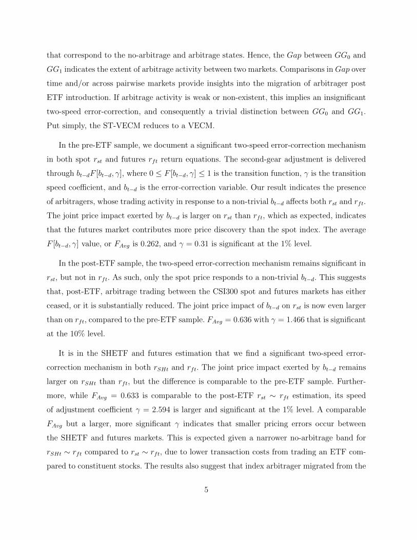
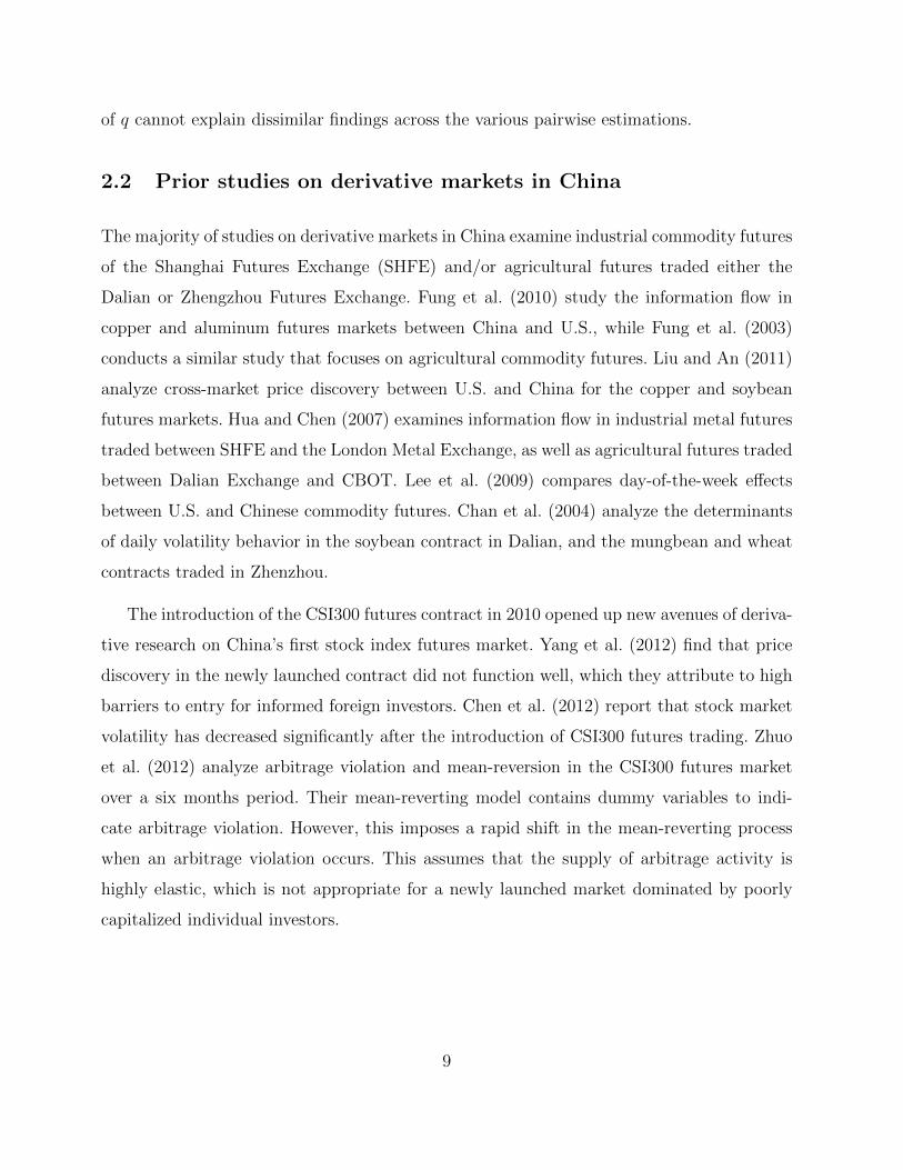
To complement the discussions thus far, we plot the estimated F [bt−d, γ] against bt−d

to acquire a sense of the range of pricing error that is associated with a second-gear error

correction mechanism. In Figures 4A∼C, the outer (blue) graph is based on the pre-ETF

estimation, which is identical across the three figures. The inner (green) graphs correspond

to the three post-ETF pairwise market estimations. Figure 4 shows that all three post-ETF

graphs are subsumed by the pre-ETF graph. This implies that full adjustments in pricing

errors occur within narrower bands post-ETF trading. This is not surprising given that the

arbitrage bounds that govern the carry-cost adjusted basis is expected to narrow substantially

post-ETF trading, due to lower transaction cost with trading ETFs.

INSERT FIGURE 4

Interestingly, the rst ∼ rft estimation exhibits the narrowest range of pricing errors in

Figure 4A. But according to Table 3, only rst exhibits a significant two-speed error-correction.

In contrast, although the rSHt ∼ rft estimation yields a significant two-speed error-correction

across both markets, Figure 4B shows the least narrowing in the range of pricing errors. We

elaborate on this in the next section. As a preview, if arbitragers migrate from the CSI300

spot market post-ETF, the index simply becomes a ‘follower’ market. When a non-trivial

bt−d occurs, rst will simply respond to rft and move towards the new futures price.

18

Furthermore, if arbitragers migrate predominately to the SHETF market, this can also

explain why Figure 4B shows the least narrowing in the range of pricing errors. Consider

when pricing errors are induced by informed futures traders attempting to discover a new

price for the CSI300. When the pricing error become profitably non-trivial, arbitragers step

in. Their trading activity by default will slow down informed traders from discovering the

new futures price. This interaction between informed traders and arbitragers can result in

a wider range of observed pricing errors compared to the CSI300 spot, where arbitragers

are absent. We formally examine this issue by analyzing and comparing the price discovery

mechanism among the four pairwise markets in the next section.

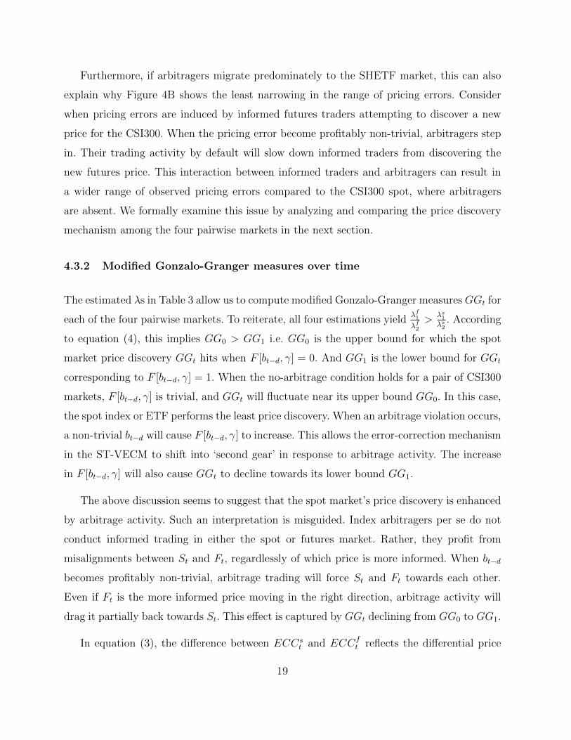
4.3.2 Modified Gonzalo-Granger measures over time

The estimated λs in Table 3 allow us to compute modified Gonzalo-Granger measures GGt for

each of the four pairwise markets. To reiterate, all four estimations yieldλf1λf2>

λs1λs2

. According

to equation (4), this implies GG0 > GG1 i.e. GG0 is the upper bound for which the spot

market price discovery GGt hits when F [bt−d, γ] = 0. And GG1 is the lower bound for GGt

corresponding to F [bt−d, γ] = 1. When the no-arbitrage condition holds for a pair of CSI300

markets, F [bt−d, γ] is trivial, and GGt will fluctuate near its upper bound GG0. In this case,

the spot index or ETF performs the least price discovery. When an arbitrage violation occurs,

a non-trivial bt−d will cause F [bt−d, γ] to increase. This allows the error-correction mechanism

in the ST-VECM to shift into ‘second gear’ in response to arbitrage activity. The increase

in F [bt−d, γ] will also cause GGt to decline towards its lower bound GG1.

The above discussion seems to suggest that the spot market’s price discovery is enhanced

by arbitrage activity. Such an interpretation is misguided. Index arbitragers per se do not

conduct informed trading in either the spot or futures market. Rather, they profit from

misalignments between St and Ft, regardlessly of which price is more informed. When bt−d

becomes profitably non-trivial, arbitrage trading will force St and Ft towards each other.

Even if Ft is the more informed price moving in the right direction, arbitrage activity will

drag it partially back towards St. This effect is captured by GGt declining from GG0 to GG1.

In equation (3), the difference between ECCst and ECCf

t reflects the differential price

19

impact exerted by bt−d on rst (or rSHt, rSZt) and rft. Arbitrage activity in response to a non-

trivial bt−d will generate more comparable price impact on both St and Ft. In the post-ETF

rst ∼ rft estimation, when F [bt−d, γ] = 0, the differential price impact is |λs1| − |λf1 | = 0.033.

This drops to |λs1 + λs2| − |λf1 + λf2 | = 0.0086, or 26%, when F [bt−d, γ] = 1. We observe

similar declines in the differential price impact to 17.3% for rSHt ∼ rft, and 16.7% for

rSZt ∼ rft, when F [bt−d, γ] increases from 0 to 1. It is noteworthy that, across all four pairwise

estimations, both GG0 and GG1 indicate that the CSI300 futures market contributes more

price discovery than each of its three spot market counterpart. This is indicated by the

magnitude of the λs from each pairwise estimation. Fluctuations in GGt between GG0 and

GG1 only reflect the extent of the futures market’s price leadership role14.

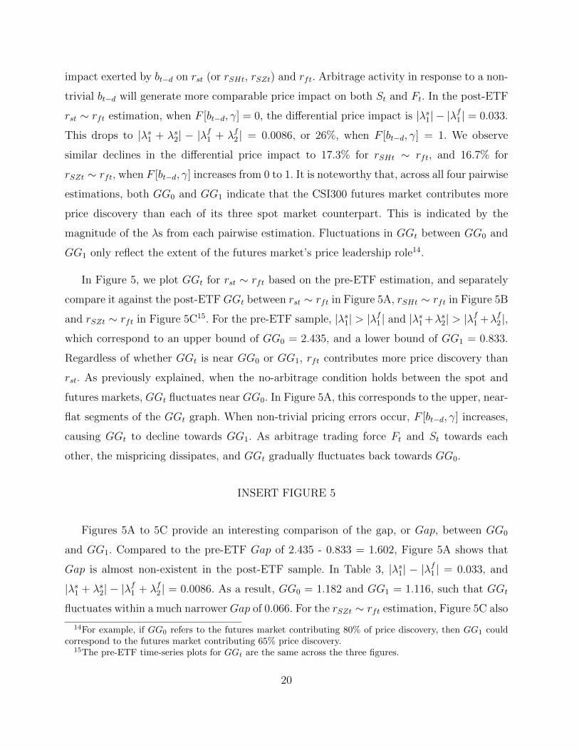
In Figure 5, we plot GGt for rst ∼ rft based on the pre-ETF estimation, and separately

compare it against the post-ETF GGt between rst ∼ rft in Figure 5A, rSHt ∼ rft in Figure 5B

and rSZt ∼ rft in Figure 5C15. For the pre-ETF sample, |λs1| > |λf1 | and |λs1 +λs2| > |λ

f1 +λf2 |,

which correspond to an upper bound of GG0 = 2.435, and a lower bound of GG1 = 0.833.

Regardless of whether GGt is near GG0 or GG1, rft contributes more price discovery than

rst. As previously explained, when the no-arbitrage condition holds between the spot and

futures markets, GGt fluctuates near GG0. In Figure 5A, this corresponds to the upper, near-

flat segments of the GGt graph. When non-trivial pricing errors occur, F [bt−d, γ] increases,

causing GGt to decline towards GG1. As arbitrage trading force Ft and St towards each

other, the mispricing dissipates, and GGt gradually fluctuates back towards GG0.

INSERT FIGURE 5

Figures 5A to 5C provide an interesting comparison of the gap, or Gap, between GG0

and GG1. Compared to the pre-ETF Gap of 2.435 - 0.833 = 1.602, Figure 5A shows that

Gap is almost non-existent in the post-ETF sample. In Table 3, |λs1| − |λf1 | = 0.033, and

|λs1 + λs2| − |λf1 + λf2 | = 0.0086. As a result, GG0 = 1.182 and GG1 = 1.116, such that GGt

fluctuates within a much narrower Gap of 0.066. For the rSZt ∼ rft estimation, Figure 5C also

14For example, if GG0 refers to the futures market contributing 80% of price discovery, then GG1 couldcorrespond to the futures market contributing 65% price discovery.

15The pre-ETF time-series plots for GGt are the same across the three figures.

20

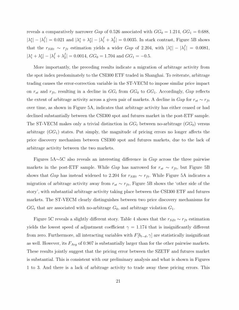
reveals a comparatively narrower Gap of 0.526 associated with GG0 = 1.214, GG1 = 0.688,

|λs1| − |λf1 | = 0.021 and |λs1 + λs2| − |λ

f1 + λf2 | = 0.0035. In stark contrast, Figure 5B shows

that the rSHt ∼ rft estimation yields a wider Gap of 2.204, with |λs1| − |λf1 | = 0.0081,

|λs1 + λs2| − |λf1 + λf2 | = 0.0014, GG0 = 1.704 and GG1 = −0.5.

More importantly, the preceding results indicate a migration of arbitrage activity from

the spot index predominately to the CSI300 ETF traded in Shanghai. To reiterate, arbitrage

trading causes the error-correction variable in the ST-VECM to impose similar price impact

on rst and rft, resulting in a decline in GGt from GG0 to GG1. Accordingly, Gap reflects

the extent of arbitrage activity across a given pair of markets. A decline in Gap for rst ∼ rft

over time, as shown in Figure 5A, indicates that arbitrage activity has either ceased or had

declined substantially between the CSI300 spot and futures market in the post-ETF sample.

The ST-VECM makes only a trivial distinction in GGt between no-arbitrage (GG0) versus

arbitrage (GG1) states. Put simply, the magnitude of pricing errors no longer affects the

price discovery mechanism between CSI300 spot and futures markets, due to the lack of

arbitrage activity between the two markets.

Figures 5A∼5C also reveals an interesting difference in Gap across the three pairwise

markets in the post-ETF sample. While Gap has narrowed for rst ∼ rft, but Figure 5B

shows that Gap has instead widened to 2.204 for rSHt ∼ rft. While Figure 5A indicates a

migration of arbitrage activity away from rst ∼ rft, Figure 5B shows the ‘other side of the

story’, with substantial arbitrage activity taking place between the CSI300 ETF and futures

markets. The ST-VECM clearly distinguishes between two price discovery mechanisms for

GGt that are associated with no-arbitrage G0, and arbitrage violation G1.

Figure 5C reveals a slightly different story. Table 4 shows that the rSZt ∼ rft estimation

yields the lowest speed of adjustment coefficient γ = 1.174 that is insignificantly different

from zero. Furthermore, all interacting variables with F [bt−d, γ] are statistically insignificant

as well. However, its FAvg of 0.907 is substantially larger than for the other pairwise markets.

These results jointly suggest that the pricing error between the SZETF and futures market

is substantial. This is consistent with our preliminary analysis and what is shown in Figures

1 to 3. And there is a lack of arbitrage activity to trade away these pricing errors. This

21

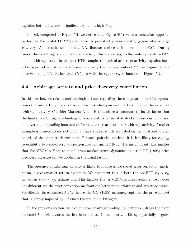
explains both a low and insignificant γ, and a high FAvg.

Indeed, compared to Figure 5B, we notice that Figure 5C reveals a somewhat opposite

pattern in the post-ETF GGt over time. A persistently non-trivial bt−d generates a large

F [bt−d, γ]. As a result, we find that GGt fluctuates close to its lower bound GG1. During

times when arbitragers are able to reduce bt−d, this allows GGt to fluctuate upwards to GG0

i.e. no-arbitrage state. In the post-ETF sample, the lack of arbitrage activity explains both

a low speed of adjustment coefficient, and why the flat segments of GGt in Figure 5C are

observed along GG1 rather than GG0, as with the rSHt ∼ rft estimation in Figure 5B.

4.4 Arbitrage activity and price discovery contribution

In this section, we raise a methodological issue regarding the computation and interpreta-

tion of cross-market price discovery measures when pairwise markets differ in the extent of

arbitrage activity. Consider Markets A and B that share a common stochastic factor, but

the limits to arbitrage are binding. One example is cross-listed stocks, where currency risk,

non-overlapping trading hour and differential tax treatment deter arbitrage activity. Another

example is ownership restriction on a firm’s stocks, which are listed on the local and foreign

boards of the same stock exchange. For such pairwise markets, it is less likely for rAt, rBt

to exhibit a two-speed error-correction mechanism. If F [bt−d, γ] is insignificant, this implies

that the VECM suffices to model cross-market return dynamics, and the GG (1995) price

discovery measure can be applied in the usual fashion.

The presence of arbitrage activity is likely to induce a two-speed error-correction mech-

anism in cross-market return dynamics. We document this in both the pre-ETF rst ∼ rft

as well as rSHt ∼ rft estimations. This implies that a VECM is misspecified since it does

not differentiate the error-correction mechanisms between no-arbitrage and arbitrage states.

Specifically, its estimated λs, λf , hence the GG (1995) measure, captures the price impact

that is jointly imposed by informed traders and arbitragers.

In the previous section, we explain how arbitrage trading, by definition, drags the more

informed Ft back towards the less informed St. Consequently, arbitrager partially negates

22

the price discovery contribution made by informed futures traders. This effect is manifested

in GGt declining from GG0 to GG1 when bt−d becomes non-trivial. Arbitrage trading, which

induces price impact on both St and Ft, cause GGt to give given an indication that price

discovery contribution by the spot (futures) market has increased (decreased). Figure 5

shows that, while this effect is consistently being observed across all four pairwise market

estimations, it is most prevalent in the pre-ETF rst ∼ rft and rSHt ∼ rft estimations. Both

estimations yield a significant two-speed error-correction mechanism in both markets, which

indicates the presence of arbitrage activity.

This raises an interesting methodological implication when using the ST-VECM’s modi-

fied GG measure to infer cross-market price discovery contribution. Put simply, it is in the

absence of arbitrage activity when we can acquire a better picture of cross-market price

discovery. In equation (3), GG0, which corresponds to F [bt−d, γ] = 0, reflects price discovery

contribution in the absence of arbitrage. To follow, GG1, which is associated with arbitrage

trading, provides a less accurate indication of cross-market price discovery.

In the context of CSI300 pairwise markets that we examined, the above distinction is

moot. This is because both GG0 and GG1 values for various pairwise markets all correspond

to the futures market contributing more price discovery than its spot market counterpart.

The magnitude of λs are consistently larger for rst, rSHt, rSZt compared to rft, regardless of

whether F [bt−d, γ] = 0 or 1. In all four pairwise estimations, Gap simply reflects the degree

of price leadership that the futures market exert on its spot market counterpart, associated

with varying degrees of arbitrage activity.

Now, let us assume a pair of markets in which the price impact by bt−d is larger for

one market when F [bt−d, γ] = 0, but it is larger for the other market when F [bt−d, γ] = 1.

Intuitively, this suggests that the ‘borderline’ GGt value16, which indicates a tie in price

discovery contribution, is straddled between GG0 and GG1. Fluctuation in GGt between

GG0 and GG1 appears to indicate an oscillation in the price leadership role between the two

markets. In fact, the price leadership role remains with the market that is indicated by GG0.

Arbitrage trading causes GGt to move from GG0 to GG1, thus giving an appearance that

16The original GG (1995) measure ranges from 0 to 1, and the borderline GG value is 0.5.

23

the other market has taken over the price leadership role.

A numerical example: To motivate the above discussion, we provide a simple numerical

example based on the λ coefficients from the pre-ETF rst ∼ rft estimation. We assume that

the estimated λf2 is -0.0103 instead of -0.0045, while the other three λs remain unchanged:

λs1 = 0.0056, λf1 = 0.0033 and λs2 = 0.0004. Based on these λ estimates, when F [bt−d, γ] = 0,

the incremental price impact on rst over rft is |λs1| − |λf1 | = 0.0056 − 0.0033 = 0.0023.

However, when F [bt−d, γ] = 1, the incremental price impact becomes |λs1 + λs2| − |λf1 + λf2 | =

0.006− 0.007 = −0.001 i.e. it is the futures market that received a larger price impact from

bt−d. Since (λs1, λf1) are unchanged, GG0 remains at 2.4348. But GG1 has decreased from

0.8333 to 0.006/(0.006+0.007)=0.4762.

More importantly, if GGt drops to GG1 = 0.8333 with λf2 = −0.0045, the futures market

still retains its price leadership role. But if GGt drops to GG1 = 0.4762, which corresponds

to a hypothetical λf2 = −0.0103, it appears that the spot index has taken over the price

leadership role. We exlain earlier that, when GG0 and GG1 give different indications on the

market that exhibits price leadership, it is GG0 that depicts a more accurate price discovery

picture. This is because GG1 incorporates the price impact of arbitrage trading.

5 Conclusion

In this paper, we find that the introduction of ETF trading does not dilute the price lead-

ership role of the CSI300 future market. CFFEX’s flagship contract still contributes more

price discovery than its three spot market counterparts. Results from the ST-VECM also

reveals that the significant two-speed error-correction mechanism in the pre-ETF rst ∼ rft

estimation is also documented in the post-ETF sample period, but only for the rSHt ∼ rft

estimation. This strongly suggests that arbitragers migrate predominately to the Huatai-

Pinebridge ETF that is traded in Shanghai.

We explain why the original GG (1995) cross-market price discovery contribution is a

noisy measure in the presence of arbitrage activity. The VECM does not formally acknowl-

edge the impact of arbitrage trading on the error-correction mechanism. Intuitively, when

24

bt−d becomes profitably non-trivial, arbitrage trading will force spot and futures prices to-

wards each other. This causes the error-correction coefficients (λs, λf ) to register comparable

price impact on rst and rft. But since arbitrage trading does not always occur, the estimated

(λs, λf ) from the VECM reflect an ‘average’ error-correction mechanism between arbitrage

and no-arbitrage states over a given sample period. Consequently, the GG (1995) measure,

which is based on (λs, λf ), is a noisy measure that encapsulates the price impact of both

informed traders as well as arbitragers.

We apply the ST-VECM to compute a modified GG measure for each of the four pairwise

market estimations. We observe that the Gap for rst ∼ rft narrows substantially when we

move from the pre-ETF to post-ETF sample. In contrast, the Gap for rSHt ∼ rft is wider

than the pre-ETF Gap for rst ∼ rft . We do not find a significant two-speed error-correction

mechanism for rSZt ∼ rft. This is consistent with earlier findings that arbitragers migrate

predominately to the SHETF. A potential mis-specification in the optimal lag dynamics for

bt−d cannot explain the dissimilar findings between SHETF and SZETF. Our diagnostic tests

confirm that both ETFs exhibit similar optimal lag structures. Furthermore, estimating a

highly non-linear ST-VECM using intraday data makes it near-infeasible to conduct a joint

estimation that encompasses all four CSI300 markets.

Indeed, we are more interested in the specific nature of the limits to arbitrage that

bind the SZETF market, but not the SHETF market. These are electronically traded close-

substitute securities, so the geographical proximity between CFFEX and Shanghai Stock Ex-

change is not a satisfying explanation for why arbitragers ignore the SZETF. Understanding

the dissimilar arbitrage situations between the two ETFs require a detailed comparison of ar-

bitrage violation characteristics, conditional on dissimilar trading or settlement features e.g.

short-interest, tracking error etc, that imposes a binding limit to arbitrage only on SZETF.

We are pursuing this direction in an on-going project.

25

References

[1] Amihud, Y., 2002. Illiquidity and stock returns: Cross-section and time serieseffects. Journal of Financial Markets 5, 31-56.

[2] Booth, R., So, W., Tse, Y., 1999. Price discovery in the German equity indexderivatives markets. Journal of Futures Markets 19, 619-643.

[3] Bose, 2007. Contribution of Indian index futures to price formation in the stockmarket. Money and Finance, 39-56.

[4] Brennan, M., Schwartz, E., 1990. Arbitrage in stock index futures. Journal ofBusiness 63, 7-32.

[5] Brenner, M., Subrahmanyam, M., Uno, J., 1989. The behavior of prices in theNikkei spot and futures market. Journal of Financial Economics 23, 363-383.

[6] Chan, K., 1992. A further analysis of the leadlag relationship between the cashmarket and stock index futures market. Review of Financial Studies 5, 123-152.

[7] Chan, K., Chan, K., Karolyi, A., 1991. Intraday volatility in the stock index andstock index futures markets. Review of Financial Studies 4, 657-684.

[8] Chan, K., Fung, H., Leung, W., 2004. Daily volatility behavior in the Chinese fu-tures markets. Journal of International Financial Markets, Institutions and Money14, 491-505.

[9] Chakravarty, S., Gulen, H., Mayhew, S., 2004. Informed trading in stock andoption markets. Journal of Finance 59, 1235-1257.

[10] Chen, H., Han, Q., Li, Y., Wu, K., 2012. Does index futures trading reduce volatil-ity in the Chinese stock market? A panel data evaluation approach. Journal ofFutures Markets 33, 1167-1190.

[11] Chu, Q., Hsieh, W., Tse, Y., 1999. Price discovery on the S&P 500 index markets:An analysis of spot index, index futures and SPDRs. International Review ofFinancial Analysis 8, 21-34.

[12] Delatte, A., Gex, M., Lpez-Villavicencio, A., 2012. Has the CDS market influencedthe borrowing cost of European countries during the sovereign crisis. Journal ofInternational Money and Finance 31, 481-497.

[13] Edwards, F., 1988. Does the futures trading increase stock market volatility. Fi-nancial Analysts Journal 44, 63-69.

[14] Fleming, J., Ostdiek, B., Whaley, R., 1996. Trading costs and the relative rates ofprice discovery in stock, futures and options markets. Journal of Futures Markets16, 353-387.

26

[15] Fung H, Leung, W., Xu, X., 2003. Information flows between the U.S. and Chinacommodity futures trading. Review of Quantitative Finance and Accounting 21,267-285.

[16] Fung, H., Liu, Q., Tse, Y., 2010. The information flow and market efficiency be-tween the US and Chinese copper and aluminum futures markets. Journal of Fu-tures Markets 30, 1192-1209.

[17] Gonzalo, J., Granger, C., 1995. Estimation of common long-memory componentsin cointegrated systems. Journal of Business and Economic Statistics 13, 27-35.

[18] Hasbrouck, J., 1995. One security, many markets: Determining the contributionsto price discovery. Journal of Finance 50, 1175-1199.

[19] Hasbrouck, J., 2003. Intraday price formation in the market for US equity indices.Journal of Finance 58, 2375-2399.

[20] Hua, H., Chen, B., 2007. International linkages of the Chinese futures markets.Applied Financial Economics 17, 1275-1287.

[21] Kawaller, I., Koch, P., Koch, T., 1987. The temporal price relationship betweenS&P 500 futures and the S&P 500 index. Journal of Finance 42, 1309-1329.

[22] Lee, K., Fung, H., Liao, T., 2009. Day-of-the-week effects in the US and Chinesecommodity futures markets. Review of Futures Markets 18, 27-53.

[23] Lim, K., 1990. Arbitrage and price behavior of Nikkei stock index futures, Journalof Futures Markets 12, 151-161.

[24] Liu, Q., An, Y., 2011. Information transmission in informationally linked markets:Evidence from US and Chinese commodity futures markets. Journal of Interna-tional Money and Finance 30, 778-795.

[25] MacKinlay, C., Ramaswamy, K., 1988. Index-futures arbitrage and the behaviorof stock index futures prices. Review of Financial Studies 1, 137-158.

[26] Miller, M., Muthuswamy, J., Whaley, R., 1994. Mean reversion of S&P500 indexbasis changes: Arbitrage-induced or statistical illusion? Journal of Finance 49,479-513.

[27] Ryoo, H., Smith, G., 2004. The impact of stock index futures on the Koren stockmarket. Applied Financial Economics 14, 243-251.

[28] So, W., Tse, Y., 2004. Pricing discovery in the Hang Seng index markets: Index,futures and the tracker fund. Journal of Futures Markets 24, 887-907.

[29] Stoll, H., Whaley, R., 1990. Stock market structure and volatility. Review of FI-nancial Studies 3, 37-71.

27

[30] Swanson, N., 1999. Finite sample properties of a simple LM test for neglectednon-linearity in error-correcting regression equations. Statistica Neerlandica 53,76-95.

[31] Taylor, N., Dijk, D., Frances, P., Lucas, A., 2000. SETS, arbitrage activity, andstock price dynamics. Journal of Banking and Finance 24, 1289-1306.

[32] Yadav, P., Pope, P., 1990. Stock index futures arbitrage: International evidence,Journal of Futures Markets 10, 573-603.

[33] Yang, J., Wang, Z., Zhou, Y., 2012. Intraday price discovery and volatility trans-mission in stock index and stock index futures markets: Evidence from China.Journal of Futures Markets 32, 99-121.

[34] Zhong, M., Darrat, A., Otero, R., 2004. Price discovery and volatility spilloversin index futures markets: Some evidence from Mexico. Journal of Banking andFinance 28, 3037-3054.

[35] Zhuo, W., Zhao, X., Zhou, Z., Wang, S., 2012. Study on stock index futures meanreversion effect and arbitrage in China based on high-frequency data. iBusiness 4,78-83.

28

Figure 1: Price series for the CSI300 spot, futures and ETF markets  

 Figure 1A: CSI300 spot and futures prices in Pre-ETF sample period Figure 1B: CSI300 spot and futures prices in Post-ETF sample period

  

   Figure 1C: SHETF and futures prices in Post-ETF sample period Figure 1D: SZETF and futures prices in Post-ETF sample period

2200

2400

2600

2800

3000

2/27/2012 3/19/2012 4/9/2012 4/30/2012 5/21/2012

Price 

2000

2200

2400

2600

2800

3000

12/3/2012 12/17/2012 12/31/2012 1/14/2013 1/28/2013

Price 

2000

2200

2400

2600

2800

3000

12/3/2012 12/24/2012 1/14/2013 2/4/2013 2/25/2013

Price 

2000

2200

2400

2600

2800

3000

12/3/2012 12/24/2012 1/14/2013 2/4/2013 2/25/2013

Price 

Figure 2: Return series for the CSI300 spot, futures and ETF markets  

    Figure 2A: CSI300 spot and futures return in pre-ETF sample period Figure 2B: CSI300 spot and futures return in post-ETF sample period

  

     Figure 2C: SHETF and futures return in post-ETF sample period Figure 2D: SZETF and futures return in post-ETF sample period

   

‐0.01

‐0.005

0

0.005

0.01

2/27/2012 3/19/2012 4/9/2012 4/30/2012 5/21/2012

Logarithm

ic re

turn

‐0.01

‐0.005

0

0.005

0.01

12/3/2012 12/17/2012 12/31/2012 1/14/2013 1/28/2013

Logarithm

ic re

turn

‐0.01

‐0.005

0

0.005

0.01

12/3/2012 12/24/2012 1/14/2013 2/4/2013 2/25/2013

Logarithm

ic re

turn

‐0.01

‐0.005

0

0.005

0.01

12/3/2012 12/24/2012 1/14/2013 2/4/2013 2/25/2013

Logarithm

ic re

turn

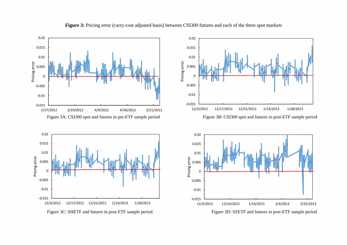
Figure 3: Pricing error (carry-cost adjusted basis) between CSI300 futures and each of the three spot markets

     Figure 3A: CSI300 spot and futures in pre-ETF sample period Figure 3B: CSI300 spot and futures in post-ETF sample period

  

       Figure 3C: SHETF and futures in post-ETF sample period Figure 3D: SZETF and futures in post-ETF sample period

‐0.015

‐0.01

‐0.005

0

0.005

0.01

0.015

0.02

2/27/2012 3/19/2012 4/9/2012 4/30/2012 5/21/2012

Pricing error 

‐0.015

‐0.01

‐0.005

0

0.005

0.01

0.015

0.02

12/3/2012 12/17/2012 12/31/2012 1/14/2013 1/28/2013

Pricing error

‐0.015

‐0.01

‐0.005

0

0.005

0.01

0.015

0.02

12/3/2012 12/17/2012 12/31/2012 1/14/2013 1/28/2013

Pricing error

‐0.015

‐0.01

‐0.005

0

0.005

0.01

0.015

0.02

12/3/2012 12/24/2012 1/14/2013 2/4/2013 2/25/2013

Pricing error

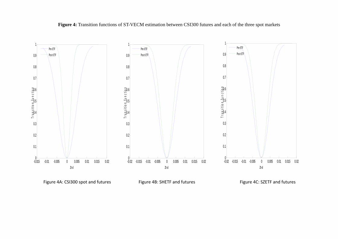
Figure 4: Transition functions of ST-VECM estimation between CSI300 futures and each of the three spot markets

      Figure 4A: CSI300 spot and futures        Figure 4B: SHETF and futures            Figure 4C: SZETF and futures    

  

   

-0.015 -0.01 -0.005 0 0.005 0.01 0.015 0.020

0.1

0.2

0.3

0.4

0.5

0.6

0.7

0.8

0.9

1

Zt‐d

Tran

sitio

n fu

nctio

n

Pre‐ETF

Post‐ETF

-0.02 -0.015 -0.01 -0.005 0 0.005 0.01 0.015 0.020

0.1

0.2

0.3

0.4

0.5

0.6

0.7

0.8

0.9

1

Zt‐d

Tran

sitio

n fu

nctio

n

Pre‐ETF

Post‐ETF

-0.02 -0.015 -0.01 -0.005 0 0.005 0.01 0.015 0.020

0.1

0.2

0.3

0.4

0.5

0.6

0.7

0.8

0.9

1

Zt‐d

Tran

sitio

n fu

nctio

n

Pre‐ETF

Post‐ETF

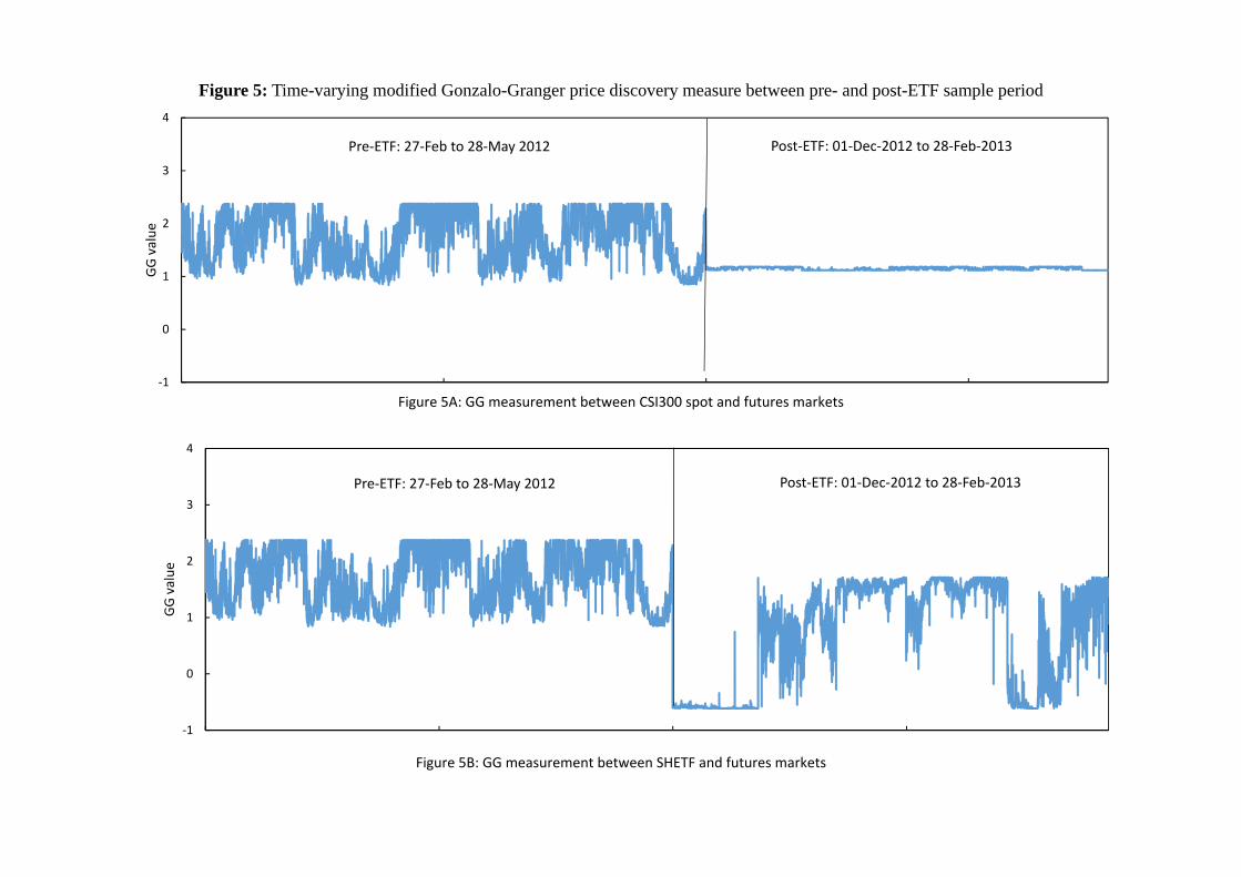
Figure 5: Time-varying modified Gonzalo-Granger price discovery measure between pre- and post-ETF sample period

 Figure 5A: GG measurement between CSI300 spot and futures markets 

 

 Figure 5B: GG measurement between SHETF and futures markets 

‐1

0

1

2

3

4

GG value

‐1

0

1

2

3

4

GG value

Pre‐ETF: 27‐Feb to 28‐May 2012  Post‐ETF: 01‐Dec‐2012 to 28‐Feb‐2013

Pre‐ETF: 27‐Feb to 28‐May 2012 Post‐ETF: 01‐Dec‐2012 to 28‐Feb‐2013

  

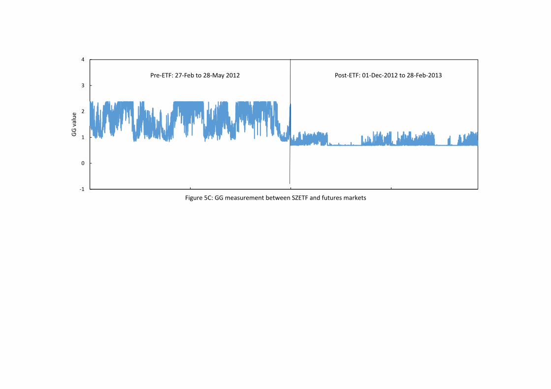
 Figure 5C: GG measurement between SZETF and futures markets 

    

‐1

0

1

2

3

4

GG value

Pre‐ETF: 27‐Feb to 28‐May 2012 Post‐ETF: 01‐Dec‐2012 to 28‐Feb‐2013

Table 1: Contractual specifications for CSI300 futures

Introduction 16th April 2010

Underlying Index China Securities Index (CSI) 300 (www.csindex.com.cn has more details)

Trading Hours SHSE and SZSE CFFEX Morning: 09:30-11:30 09:15-11:30 Afternoon: 13:00-15:00 13:00-15:15 (15:00 on last trading day)

Delivery Months and Expiry Day

Current month; Next month; Next two quarter months; Third Friday of a given delivery month

Contract and Tick Size 300 RMB per index point; 0.2 index point or 60 RMB tick

Price Limits ±10% on the previous trading day’s settlement price

Daily Settlement Price Positions are cash-settled. The settlement price is calculated as the volume-weighted average price (VWAP) for a given contract over a certain period of time for that trading day.

Trading Platform Double-auction electronic limit order book

 

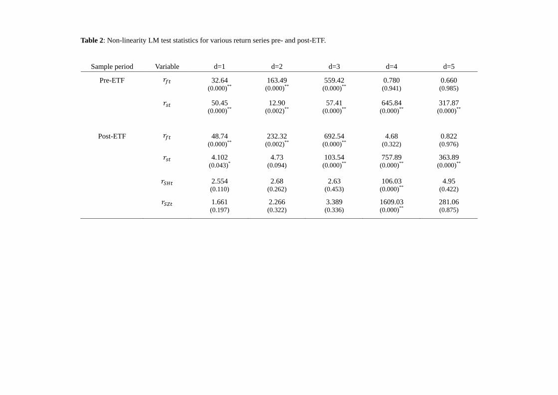
Table 2: Non-linearity LM test statistics for various return series pre- and post-ETF.

Sample period Variable d=1 d=2 d=3 d=4 d=5

Pre-ETF 32.64 163.49 559.42 0.780 0.660 (0.000)** (0.000)** (0.000)** (0.941) (0.985)

50.45 12.90 57.41 645.84 317.87 (0.000)** (0.002)** (0.000)** (0.000)** (0.000)**

Post-ETF 48.74 232.32 692.54 4.68 0.822 (0.000)** (0.002)** (0.000)** (0.322) (0.976)

4.102 4.73 103.54 757.89 363.89 (0.043)* (0.094) (0.000)** (0.000)** (0.000)**

2.554 2.68 2.63 106.03 4.95 (0.110) (0.262) (0.453) (0.000)** (0.422)

1.661 2.266 3.389 1609.03 281.06 (0.197) (0.322) (0.336) (0.000)** (0.875)

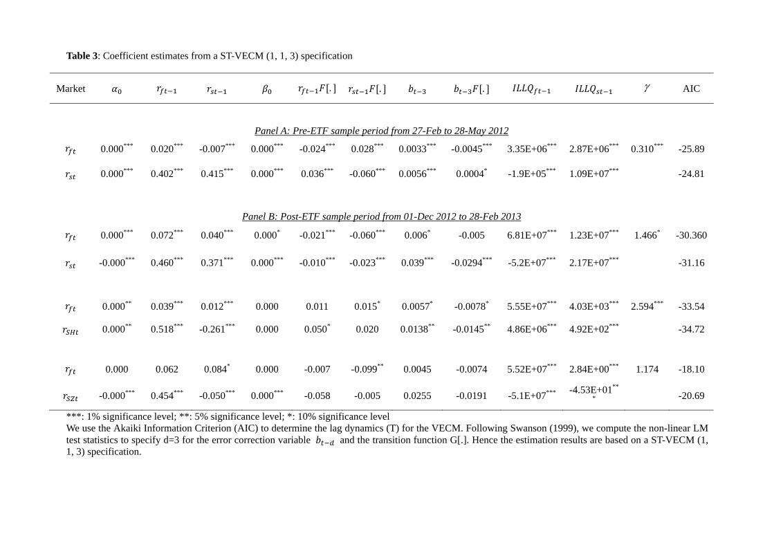
Table 3: Coefficient estimates from a ST-VECM (1, 1, 3) specification

Market . . . AIC

Panel A: Pre-ETF sample period from 27-Feb to 28-May 2012

0.000*** 0.020*** -0.007*** 0.000*** -0.024*** 0.028*** 0.0033*** -0.0045*** 3.35E+06*** 2.87E+06*** 0.310*** -25.89

0.000*** 0.402*** 0.415*** 0.000*** 0.036*** -0.060*** 0.0056*** 0.0004* -1.9E+05*** 1.09E+07*** -24.81

Panel B: Post-ETF sample period from 01-Dec 2012 to 28-Feb 2013

0.000*** 0.072*** 0.040*** 0.000* -0.021*** -0.060*** 0.006* -0.005 6.81E+07*** 1.23E+07*** 1.466* -30.360

-0.000*** 0.460*** 0.371*** 0.000*** -0.010*** -0.023*** 0.039*** -0.0294*** -5.2E+07*** 2.17E+07*** -31.16

0.000** 0.039*** 0.012*** 0.000 0.011 0.015* 0.0057* -0.0078* 5.55E+07*** 4.03E+03*** 2.594*** -33.54

0.000** 0.518*** -0.261*** 0.000 0.050* 0.020 0.0138** -0.0145** 4.86E+06*** 4.92E+02*** -34.72

0.000 0.062 0.084* 0.000 -0.007 -0.099** 0.0045 -0.0074 5.52E+07*** 2.84E+00*** 1.174 -18.10

-0.000*** 0.454*** -0.050*** 0.000*** -0.058 -0.005 0.0255 -0.0191 -5.1E+07*** -4.53E+01**

* -20.69

***: 1% significance level; **: 5% significance level; *: 10% significance level We use the Akaiki Information Criterion (AIC) to determine the lag dynamics (T) for the VECM. Following Swanson (1999), we compute the non-linear LM test statistics to specify d=3 for the error correction variable and the transition function G[.]. Hence the estimation results are based on a ST-VECM (1, 1, 3) specification.

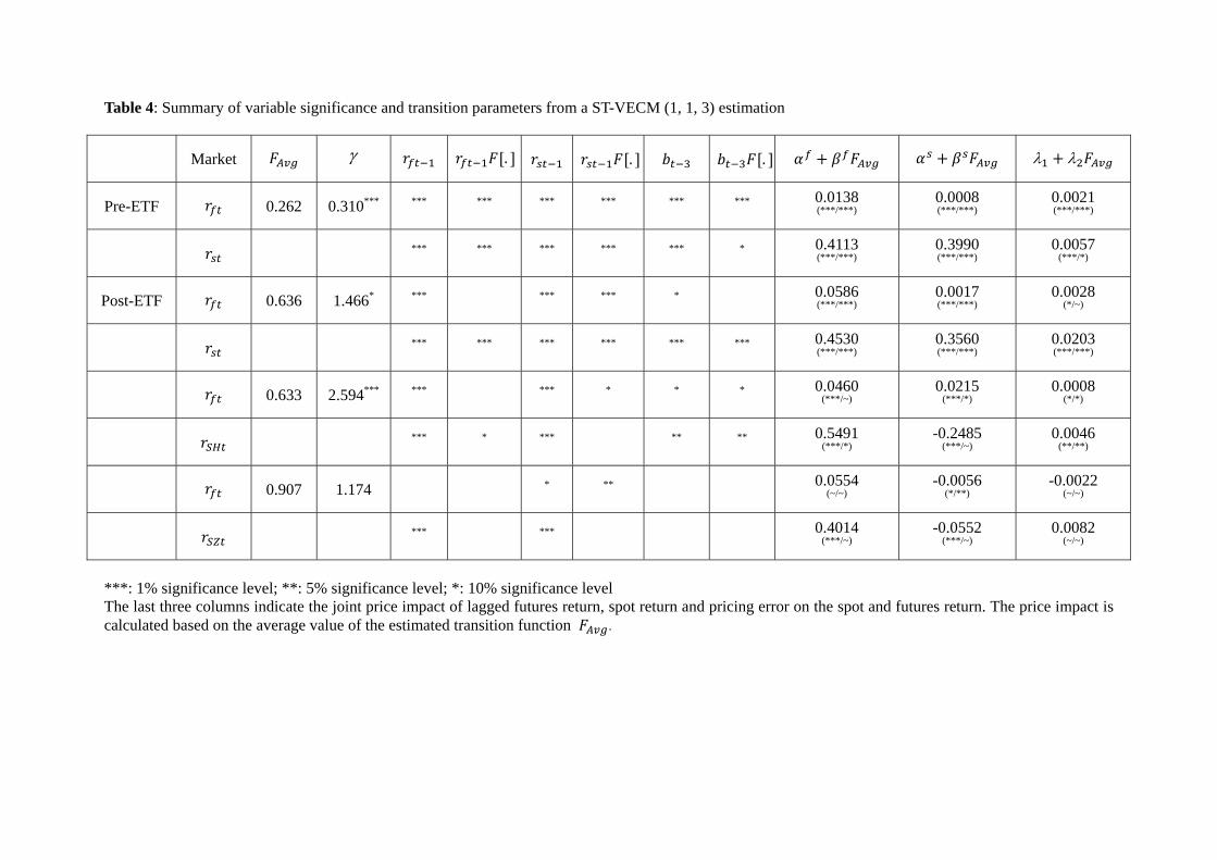
Table 4: Summary of variable significance and transition parameters from a ST-VECM (1, 1, 3) estimation

  Market       .   . .

Pre-ETF 0.262 0.310*** *** *** *** *** *** *** 0.0138 (***/***)

0.0008 (***/***)

0.0021 (***/***)

*** *** *** *** *** * 0.4113 (***/***)

0.3990 (***/***)

0.0057 (***/*)

Post-ETF 0.636 1.466* *** *** *** * 0.0586 (***/***)

0.0017 (***/***)

0.0028 (*/~)

    *** *** *** *** *** *** 0.4530 (***/***)

0.3560 (***/***)

0.0203 (***/***)

  0.633 2.594*** *** *** * * * 0.0460 (***/~)

0.0215 (***/*)

0.0008 (*/*)

    *** * *** ** ** 0.5491 (***/*)

-0.2485 (***/~)

0.0046 (**/**)

  0.907 1.174 * ** 0.0554 (~/~)

-0.0056 (*/**)

-0.0022 (~/~)

    *** *** 0.4014 (***/~)

-0.0552 (***/~)

0.0082 (~/~)

***: 1% significance level; **: 5% significance level; *: 10% significance level The last three columns indicate the joint price impact of lagged futures return, spot return and pricing error on the spot and futures return. The price impact is calculated based on the average value of the estimated transition function .