Embed Size (px)
Citation preview
Graduate Theses and Dissertations Iowa State University Capstones, Theses andDissertations
2008
Architecture and debugging of digital signalprocessing software in a high frequency MIL-STD-188-110A single tone receiverJanette Marie Eberhard ProvoltIowa State University
Follow this and additional works at: https://lib.dr.iastate.edu/etd
Part of the Electrical and Computer Engineering Commons
This Thesis is brought to you for free and open access by the Iowa State University Capstones, Theses and Dissertations at Iowa State University DigitalRepository. It has been accepted for inclusion in Graduate Theses and Dissertations by an authorized administrator of Iowa State University DigitalRepository. For more information, please contact [email protected].
Recommended CitationProvolt, Janette Marie Eberhard, "Architecture and debugging of digital signal processing software in a high frequency MIL-STD-188-110A single tone receiver" (2008). Graduate Theses and Dissertations. 10873.https://lib.dr.iastate.edu/etd/10873
Architecture and debugging of digital signal processing software in
a high frequency MIL-STD-188-110A single tone receiver
by
Janette Marie Eberhard Provolt
A thesis submitted to the graduate faculty
in partial fulfillment of the requirements for the degree of
MASTER OF SCIENCE
Major: Electrical Engineering
Program of Study Committee:Zhengdao Wang, Major Professor
Robert WeberAleksandar Dogandzic
Iowa State University
Ames, Iowa
2008
Copyright c© Janette Marie Eberhard Provolt, 2008. All rights reserved.

ii
DEDICATION
This thesis is dedicated to my wonderful husband, Brandon. Without his love, help and
encouragement I would not have been able to complete this work. I am also dedicating this to
my family and friends for their love, understanding and support throughout graduate school.
Finally, this thesis is dedicated to my undergraduate professors Dr. Roger Green and the
late Floyd Patterson for their guidance and encouragement to further my education, and for
sparking my interest in signal processing.
iii
TABLE OF CONTENTS
LIST OF FIGURES . . . . . . . . . . . . . . . . . . . . . . . . . . . . . . . . . . v
LIST OF TABLES . . . . . . . . . . . . . . . . . . . . . . . . . . . . . . . . . . . vii
ABSTRACT . . . . . . . . . . . . . . . . . . . . . . . . . . . . . . . . . . . . . . . viii
CHAPTER 1. INTRODUCTION . . . . . . . . . . . . . . . . . . . . . . . . . 1
1.1 HF Communication Challenges . . . . . . . . . . . . . . . . . . . . . . . . . . . 1
1.2 HF Communication History . . . . . . . . . . . . . . . . . . . . . . . . . . . . . 5
1.3 Performance Requirements . . . . . . . . . . . . . . . . . . . . . . . . . . . . . 6
1.4 Organization of the Thesis . . . . . . . . . . . . . . . . . . . . . . . . . . . . . . 8
CHAPTER 2. MIL-STD-188-110A SINGLE-TONE MODEM . . . . . . . . 9
2.1 Over-the-air Specifications . . . . . . . . . . . . . . . . . . . . . . . . . . . . . . 9
2.2 Top Level Transmit Data Processing . . . . . . . . . . . . . . . . . . . . . . . . 12
CHAPTER 3. CHANNEL MODEL AND RECEIVE PATH . . . . . . . . . 19
3.1 Equivalent Channel Model . . . . . . . . . . . . . . . . . . . . . . . . . . . . . . 21
3.2 Common Functionality . . . . . . . . . . . . . . . . . . . . . . . . . . . . . . . . 22
3.3 Preamble Functionality . . . . . . . . . . . . . . . . . . . . . . . . . . . . . . . 24
3.3.1 Preamble Acquisition Mode . . . . . . . . . . . . . . . . . . . . . . . . . 25
3.3.2 Preamble Tracking Mode . . . . . . . . . . . . . . . . . . . . . . . . . . 26
3.3.3 End of Preamble Mode . . . . . . . . . . . . . . . . . . . . . . . . . . . 28
3.4 Data/Probe Functionality . . . . . . . . . . . . . . . . . . . . . . . . . . . . . . 28
3.4.1 Probe Correlators . . . . . . . . . . . . . . . . . . . . . . . . . . . . . . 29
3.4.2 Channel Estimate . . . . . . . . . . . . . . . . . . . . . . . . . . . . . . 32
iv
3.4.3 Matched Filter, Equalizer, and Demodulator . . . . . . . . . . . . . . . 33
3.4.4 Deinterleaver, Decoder, and EOM Detector . . . . . . . . . . . . . . . . 41
CHAPTER 4. ISOLATION OF THE SOFTWARE DEFECT USING BIT
ERROR TIMING AND CHANNEL EFFECTS . . . . . . . . . . . . . . . 42
4.1 Software Isolation using Bit Error Timing . . . . . . . . . . . . . . . . . . . . . 42
4.1.1 Errors at the Beginning of the Reception . . . . . . . . . . . . . . . . . 42
4.1.2 Errors at the End of the Reception . . . . . . . . . . . . . . . . . . . . . 46
4.1.3 Errors Throughout the Reception . . . . . . . . . . . . . . . . . . . . . . 47
4.2 Software Isolation using Channel Effects . . . . . . . . . . . . . . . . . . . . . . 48
4.2.1 Doppler Isolation . . . . . . . . . . . . . . . . . . . . . . . . . . . . . . . 49
4.2.2 Terminal Clock Difference Isolation . . . . . . . . . . . . . . . . . . . . . 52
4.2.3 Noise Isolation . . . . . . . . . . . . . . . . . . . . . . . . . . . . . . . . 54
4.2.4 Frequency Dispersion Isolation . . . . . . . . . . . . . . . . . . . . . . . 57
4.2.5 Time Dispersion Isolation . . . . . . . . . . . . . . . . . . . . . . . . . . 61
4.3 Software Isolation Summary . . . . . . . . . . . . . . . . . . . . . . . . . . . . . 68
CHAPTER 5. SUMMARY AND FUTURE WORK . . . . . . . . . . . . . . 71
APPENDIX
ACRONYNMS . . . . . . . . . . . . . . . . . . . . . . . . . . . . . . . . . . . 73
BIBLIOGRAPHY . . . . . . . . . . . . . . . . . . . . . . . . . . . . . . . . . . . 75
ACKNOWLEDGEMENTS . . . . . . . . . . . . . . . . . . . . . . . . . . . . . . 76
v
LIST OF FIGURES
Figure 1.1 Frequency Dispersion of 3 Hz . . . . . . . . . . . . . . . . . . . . . . . 3
Figure 1.2 Multipath . . . . . . . . . . . . . . . . . . . . . . . . . . . . . . . . . . 4
Figure 1.3 Fading Caused by Time Dispersion . . . . . . . . . . . . . . . . . . . . 4
Figure 2.1 Single Tone Over-the-Air Structure . . . . . . . . . . . . . . . . . . . . 10
Figure 2.2 Detailed Transmit Block Diagram . . . . . . . . . . . . . . . . . . . . . 13
Figure 2.3 Interleaver Example . . . . . . . . . . . . . . . . . . . . . . . . . . . . . 14
Figure 2.4 Constellation Diagram of the Modulator Output . . . . . . . . . . . . . 15
Figure 2.5 Frequency Domain of the Waveshaper Output . . . . . . . . . . . . . . 16
Figure 2.6 Frequency Domain of the Translator Output . . . . . . . . . . . . . . . 17
Figure 2.7 Quadrature Mix performed by the FPGA . . . . . . . . . . . . . . . . 18
Figure 3.1 Receive Block Diagram . . . . . . . . . . . . . . . . . . . . . . . . . . . 19
Figure 3.2 HF Radio Receive Signal Processing Functionality . . . . . . . . . . . . 20
Figure 3.3 Channel Model . . . . . . . . . . . . . . . . . . . . . . . . . . . . . . . 21
Figure 3.4 Single Tone Receive Common Functionality . . . . . . . . . . . . . . . 22
Figure 3.5 Receive Waveshaper Block Diagram . . . . . . . . . . . . . . . . . . . . 23
Figure 3.6 Simplified Channel Model . . . . . . . . . . . . . . . . . . . . . . . . . 24
Figure 3.7 Single Tone Receive Preamble Functionality . . . . . . . . . . . . . . . 25
Figure 3.8 Single Tone Receive Data Functionality . . . . . . . . . . . . . . . . . . 29
Figure 3.9 Probe Correlators . . . . . . . . . . . . . . . . . . . . . . . . . . . . . . 30
Figure 3.10 Probe Correlation with 4 Sample Positions . . . . . . . . . . . . . . . . 31
Figure 3.11 LMS Algorithm . . . . . . . . . . . . . . . . . . . . . . . . . . . . . . . 32
vi
Figure 3.12 Matched Filter at the Receiver . . . . . . . . . . . . . . . . . . . . . . 34
Figure 3.13 Matched Filter and Zero-Forcing Decision Feedback Equalizer . . . . . 35
Figure 4.1 Frequency Domain of the Translator Output with 0 and 70 Hz Doppler 50
Figure 4.2 Acquisition FFT Output with 0 and 70 Hz Doppler . . . . . . . . . . . 51
Figure 4.3 Original Probe Correlation and after Drift . . . . . . . . . . . . . . . . 53
Figure 4.4 Equalzied Constellation Diagram with 40 dB and 15 dB SNR . . . . . 56
Figure 4.5 Average Incoming Magnitude with 0 and 5 Hz of Frequency Dispersion 58
Figure 4.6 Average Incoming Magnitude and Corresponding Bit Errors with 5 Hz
of Frequency Dispersion . . . . . . . . . . . . . . . . . . . . . . . . . . 59
Figure 4.7 Average Incoming Magnitude and Corresponding Bit Errors with 0.5
Hz of Frequency Dispersion . . . . . . . . . . . . . . . . . . . . . . . . 60
Figure 4.8 Probe Correlation with 0 msec and 5 msec of Time Dispersion . . . . . 62
Figure 4.9 Probe Correlation with 2 msec and 5 msec of Time Dispersion . . . . . 63
Figure 4.10 Probe Correlation with 5 dB and 0 dB Power Difference . . . . . . . . 66
Figure 4.11 Unequalized and Equalized Constellation Diagrams with 2 msec of Time
Dispersion . . . . . . . . . . . . . . . . . . . . . . . . . . . . . . . . . . 67
Figure 4.12 Unequalized and Equalized Constellation Diagrams with 5 msec of Time
Dispersion and 1 Hz of Frequency Dispersion . . . . . . . . . . . . . . 68
vii
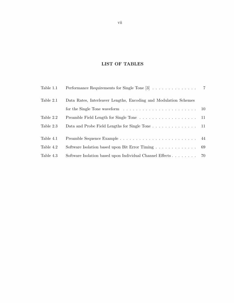
LIST OF TABLES
Table 1.1 Performance Requirements for Single Tone [3] . . . . . . . . . . . . . . 7
Table 2.1 Data Rates, Interleaver Lengths, Encoding and Modulation Schemes
for the Single Tone waveform . . . . . . . . . . . . . . . . . . . . . . . 10
Table 2.2 Preamble Field Length for Single Tone . . . . . . . . . . . . . . . . . . 11
Table 2.3 Data and Probe Field Lengths for Single Tone . . . . . . . . . . . . . . 11
Table 4.1 Preamble Sequence Example . . . . . . . . . . . . . . . . . . . . . . . . 44
Table 4.2 Software Isolation based upon Bit Error Timing . . . . . . . . . . . . . 69
Table 4.3 Software Isolation based upon Individual Channel Effects . . . . . . . . 70
viii
ABSTRACT
The MIL-STD-188-110A Single Tone high frequency modem is used by the United States
military everyday as a beyond line-of-sight radio. Typically, beyond line-of-sight military
radios use satellites for reflection. Satellite time is in high demand, and since there are a
finite number of satellites in orbit, it makes over-the-air time expensive. The Single Tone high
frequency modem offers a reliable alternative by using the ionosphere, rather than a satellite, for
reflection. The ionosphere adds unique channel effects, causing the signal processing software
to be more complex and harder to debug than radios which use satellites.
Before being placed into production, the MIL-STD-188-110A Single Tone high frequency
modem is placed under comprehensive performance tests. These tests are meant to fully verify
all aspects of the software and to impose all possible channel effects such as additive white
Gaussian noise, doppler shift, terminal clock differences, frequency and time dispersion. When
a test fails, debugging the software can be tedious and time consuming. The two major steps to
quick and successful debugging are understanding and isolation. The engineer must understand
the channel model and receive path in order to correlate a test failure with a specific section
of software. After the channel model and receive path are understood, timing patterns of
bit errors and test failures caused by individual channel effects help the engineer isolate the
software defect. This thesis compiles the necessary information to understand a generalized
receive path and provides a framework for isolating a software defect.
1
CHAPTER 1. INTRODUCTION
There are many types of over-the-air communications used by the United States military
today, and many are able to transmit beyond line-of-sight (LOS), but most require the use
of a satellite for reflection. Since satellites are expensive to launch and maintain, there are a
finite number of satellites in orbit, which makes satellite time high in demand and expensive
to use. High frequency (HF) offers an alternative for beyond LOS communication. HF uses
frequencies between 3 MHz and 30 MHz and relies on the earth’s ionosphere for reflection,
making beyond LOS communication possible without the use of a satellite.
Some typical challenges associated with over-the-air communication include noise, doppler
shift, and terminal clock differences. HF communication also encounters challenges associated
specifically with the use of the ionosphere. According to Furman and Nieto, “The HF channel
is characterized as a multi-path time-varying environment that produces time and frequency
dispersion.” [6]. Frequency and time dispersion add to the complexity of the signal processing
in HF radios. With the added complexity, it can be very difficult to isolate issues seen during
performance testing. This thesis provides a matrix of information to help isolate a software
defect.
1.1 HF Communication Challenges
Noise, doppler shift, and terminal clock differences occur with every over-the-air transmis-
sion, regardless of whether or not the ionosphere is used for reflection. Noise occurs over any
channel and can be thought of as a source of an additive random signal. In most cases, the
noise is assumed to be additive white Gaussian noise (AWGN). Many waveforms require a
minimum signal-to-noise ratio (SNR) to acknowledge a signal. If the noise power is too high
2
with respect to the signal power, the minimum SNR is not met and the receiving terminal does
not detect the signal.
Doppler shift is caused by the relative movement of either the transmitting or receiving
terminal. It causes the receiving terminal to detect a signal that is shifted in frequency from
the expected carrier. Many waveforms have a maximum doppler shift setting for which they
correct. If the doppler shift detected is greater than this limit, the receiving terminal corrects
for the maximum doppler shift and some amount of uncorrected frequency offset remains in
the signal. This causes bit errors or a potential loss of signal.
Timing differences between the transmitting and receiving terminals are caused by the
internal clocks. If the clock on the transmitting terminal is faster or slower than the clock
on the receiving terminal, the receiving terminal slowly sees the received signal drift. If not
addressed by the receiver, this eventually causes bit errors and a loss of signal.
Frequency and time dispersion occur with communications which use the ionosphere for
reflection. Ionospheric fading occurs when the ionosphere absorbs signal energy during trans-
mission. The ionosphere absorbs signal energy at different rates, depending on the density
of the ionosphere. According to Nieto, since the density of the ionosphere is not constant or
predictable, it is impossible to find a “fixed relationship between distance and signal strength
for ionospheric propagation” [1]. Since the rate at which energy is absorbed is not constant,
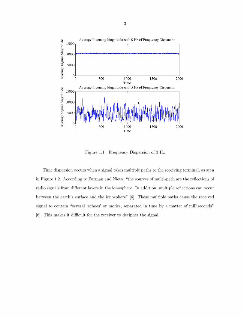
it causes frequency dispersion. The top image in Figure 1.1 shows the average incoming am-
plitude with no frequency dispersion, and the bottom image shows the effects of frequency
dispersion.
3
Figure 1.1 Frequency Dispersion of 3 Hz
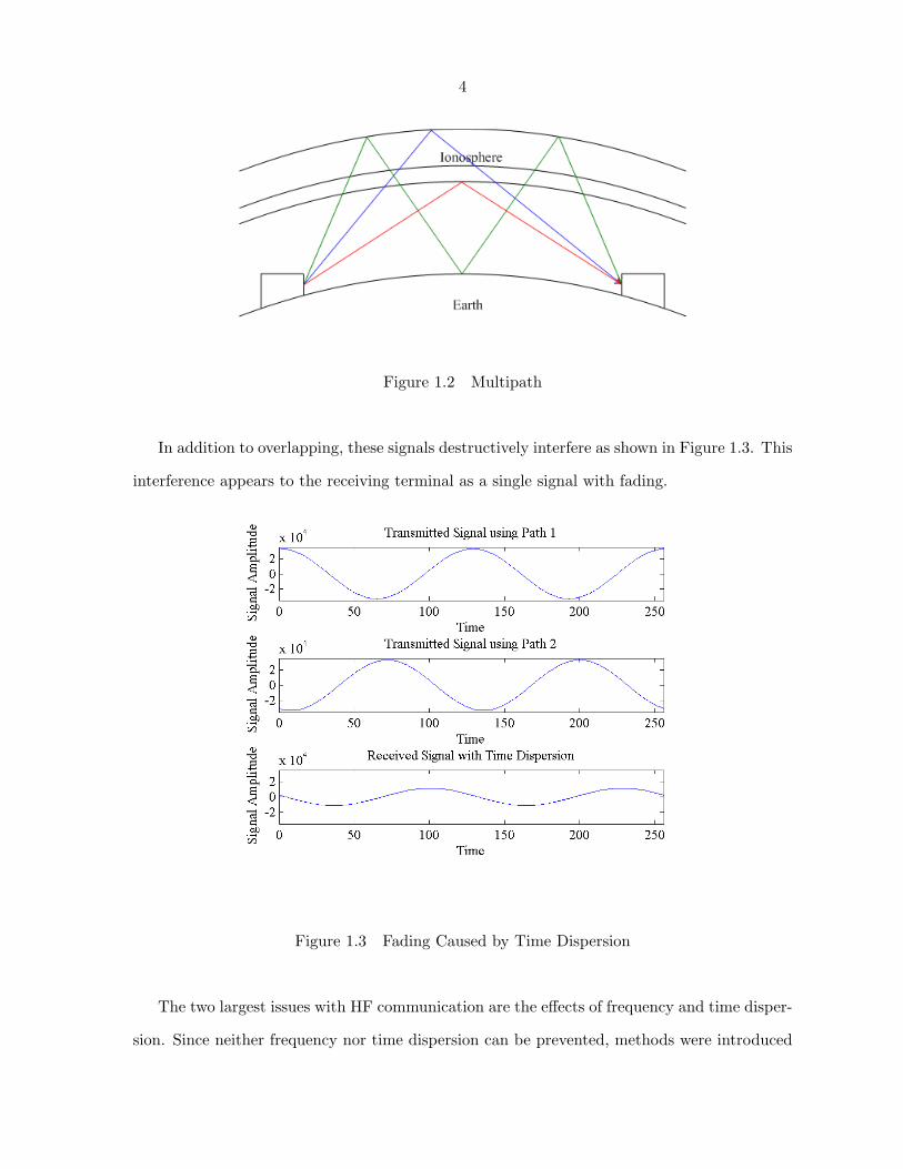
Time dispersion occurs when a signal takes multiple paths to the receiving terminal, as seen
in Figure 1.2. According to Furman and Nieto, “the sources of multi-path are the reflections of
radio signals from different layers in the ionosphere. In addition, multiple reflections can occur
between the earth’s surface and the ionosphere” [6]. These multiple paths cause the received
signal to contain “several ‘echoes’ or modes, separated in time by a matter of milliseconds”
[6]. This makes it difficult for the receiver to decipher the signal.
4
Figure 1.2 Multipath
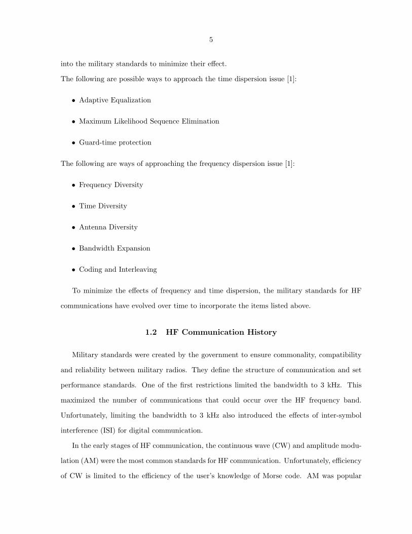
In addition to overlapping, these signals destructively interfere as shown in Figure 1.3. This
interference appears to the receiving terminal as a single signal with fading.
Figure 1.3 Fading Caused by Time Dispersion
The two largest issues with HF communication are the effects of frequency and time disper-
sion. Since neither frequency nor time dispersion can be prevented, methods were introduced
5
into the military standards to minimize their effect.
The following are possible ways to approach the time dispersion issue [1]:
• Adaptive Equalization
• Maximum Likelihood Sequence Elimination
• Guard-time protection
The following are ways of approaching the frequency dispersion issue [1]:
• Frequency Diversity
• Time Diversity
• Antenna Diversity
• Bandwidth Expansion
• Coding and Interleaving
To minimize the effects of frequency and time dispersion, the military standards for HF
communications have evolved over time to incorporate the items listed above.
1.2 HF Communication History
Military standards were created by the government to ensure commonality, compatibility
and reliability between military radios. They define the structure of communication and set
performance standards. One of the first restrictions limited the bandwidth to 3 kHz. This
maximized the number of communications that could occur over the HF frequency band.
Unfortunately, limiting the bandwidth to 3 kHz also introduced the effects of inter-symbol
interference (ISI) for digital communication.
In the early stages of HF communication, the continuous wave (CW) and amplitude modu-
lation (AM) were the most common standards for HF communication. Unfortunately, efficiency
of CW is limited to the efficiency of the user’s knowledge of Morse code. AM was popular
6
because the implementation simplicity is comparable to CW, and it has the advantage that the
user does not have to be familiar with Morse code. The disadvantage to AM is the bandwidth
inefficiency. According to the HF Communications Data Book, the AM waveform “occupies a
wide spectrum and is inefficient in the sense that a great deal of unneeded carrier (5 kHz) is
generated to carry the modulation” [2]. To eliminate this inefficiency, single sideband (SSB)
waveforms were created. A SSB waveform carries the same amount of information as a double
sideband (DSB) waveform, but only transmits the upper sideband (USB) or lower sideband
(LSB), greatly reducing the needed bandwidth. One of the first standardized waveforms to use
the SSB idea was the frequency shift keying (FSK) waveform described in MIL-STD-188-110B.
Even though SSB FSK is more efficient than the previous methods, it still battles relia-
bility issues caused by frequency and time dispersion. According to the HF Communications
Data Book, “spatial diversity and frequency diversity were commonly used to improve the
reliability. However, due to bandwidth and resource limitations,” [2] another standardized
waveform, Single Tone, was introduced and can be found in MIL-STD-188-110A. The Sin-
gle Tone waveform still uses SSB for bandwidth efficiency, but instead of using spatial and
frequency diversity to battle frequency and time dispersion as FSK does, it uses encoding,
interleaving, and equalization. Single Tone will be the HF waveform focus for the remainder
of this thesis.
1.3 Performance Requirements
Interoperability is ensured in all military radios through the use of military standards. The
Single Tone modem performance standard requires that a receiver must be able to detect and
correct for a maximum doppler shift of 75 Hz [3]. There is not a specific performance require-
ment pertaining to terminal clock differences, but the modem must implement a mechanism to
correct for clock differences in order to communicate with other radios for several consecutive
hours.
In addition to doppler shift, the military standard also sets requirements for noise, frequency
and time dispersion and can be seen in Table 1.1. These standards require that a minimum
7
bit error rate (BER) be met under certain channel conditions. The military standards use the
Watterson model as a channel simulator and a way to standardize the BER performance.
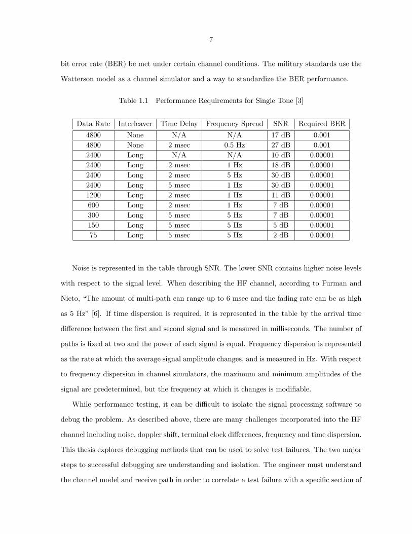
Table 1.1 Performance Requirements for Single Tone [3]
Data Rate Interleaver Time Delay Frequency Spread SNR Required BER
4800 None N/A N/A 17 dB 0.0014800 None 2 msec 0.5 Hz 27 dB 0.0012400 Long N/A N/A 10 dB 0.000012400 Long 2 msec 1 Hz 18 dB 0.000012400 Long 2 msec 5 Hz 30 dB 0.000012400 Long 5 msec 1 Hz 30 dB 0.000011200 Long 2 msec 1 Hz 11 dB 0.00001600 Long 2 msec 1 Hz 7 dB 0.00001300 Long 5 msec 5 Hz 7 dB 0.00001150 Long 5 msec 5 Hz 5 dB 0.0000175 Long 5 msec 5 Hz 2 dB 0.00001
Noise is represented in the table through SNR. The lower SNR contains higher noise levels
with respect to the signal level. When describing the HF channel, according to Furman and
Nieto, “The amount of multi-path can range up to 6 msec and the fading rate can be as high
as 5 Hz” [6]. If time dispersion is required, it is represented in the table by the arrival time
difference between the first and second signal and is measured in milliseconds. The number of
paths is fixed at two and the power of each signal is equal. Frequency dispersion is represented
as the rate at which the average signal amplitude changes, and is measured in Hz. With respect
to frequency dispersion in channel simulators, the maximum and minimum amplitudes of the
signal are predetermined, but the frequency at which it changes is modifiable.
While performance testing, it can be difficult to isolate the signal processing software to
debug the problem. As described above, there are many challenges incorporated into the HF
channel including noise, doppler shift, terminal clock differences, frequency and time dispersion.
This thesis explores debugging methods that can be used to solve test failures. The two major
steps to successful debugging are understanding and isolation. The engineer must understand
the channel model and receive path in order to correlate a test failure with a specific section of
8
software. After the channel model and receive path are understood, the isolation of a software
defect through timing patterns of bit errors and individual channel effects is possible.
1.4 Organization of the Thesis
This thesis is organized in the following manner.
• Chapter 1 explains why HF communications are used and the challenges associated with
the HF channel. It also describes how the military standards have evolved over time
to minimize some of these challenges. Performance requirements, set by the military
standard, are also discussed.
• Chapter 2 presents the over-the-air specifications for the Single Tone HF waveform. Also
discussed is a high level overview of the transmit data processing.
• Chapter 3 explains the channel model and the entire receive path.
• Chapter 4 explains methods of isolating a software defect through timing patterns of bit
errors and individual channel effects.
• Chapter 5 summarizes the thesis and suggests future work.
9
CHAPTER 2. MIL-STD-188-110A SINGLE-TONE MODEM
There are many different types of signal processing the HF waveform uses to communicate
signals over-the-air. Each type of processing produces a unique waveform, as described in
their respective military standards. This chapter contains an overview of the over-the-air
specifications for the Single Tone HF waveform, as described in MIL-STD-188-110A [3]. Also
discussed is a high level overview of the transmit data processing.
2.1 Over-the-air Specifications
The Single Tone waveform converts binary information into a single M-ary phase shift
keying (PSK) modulated output carrier and is described in MIL-STD-188-110A [3]. The
possible data rates defined for the Single Tone waveform are 75, 150, 300, 600, 1200, 2400,
and 4800 bits per second (bps). A forward error correction (FEC) encoding rate of 12 is used
along with an interleaver to minimize bit errors. The possible interleaver lengths are 0.6 and
4.8 seconds. Since interleaving comes before modulation, the length of the interleaver (in bits)
varies, depending on the data rate. See table 2.1 for a complete list of possible combinations
of data rates, interleaver lengths, encoding and modulation schemes.
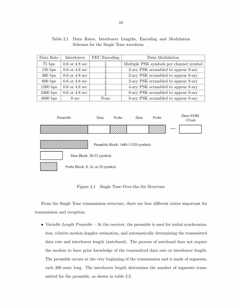
Figure 2.1 illustrates the structure of a Single Tone transmission. The major components
within the transmission structure are preamble, data and probe blocks. Contained within the
last data blocks are the EOM and flush.
10
Table 2.1 Data Rates, Interleaver Lengths, Encoding and ModulationSchemes for the Single Tone waveform
Data Rate Interleaver FEC Encoding Data Modulation
75 bps 0.6 or 4.8 sec 12 Multiple PSK symbols per channel symbol
150 bps 0.6 or 4.8 sec 12 2-ary PSK scrambled to appear 8-ary
300 bps 0.6 or 4.8 sec 12 2-ary PSK scrambled to appear 8-ary
600 bps 0.6 or 4.8 sec 12 2-ary PSK scrambled to appear 8-ary
1200 bps 0.6 or 4.8 sec 12 4-ary PSK scrambled to appear 8-ary
2400 bps 0.6 or 4.8 sec 12 8-ary PSK scrambled to appear 8-ary
4800 bps 0 sec None 8-ary PSK scrambled to appear 8-ary
Figure 2.1 Single Tone Over-the-Air Structure
From the Single Tone transmission structure, there are four different states important for
transmission and reception:
• Variable Length Preamble – At the receiver, the preamble is used for initial synchroniza-
tion, relative motion doppler estimation, and automatically determining the transmitted
data rate and interleaver length (autobaud). The process of autobaud does not require
the modem to have prior knowledge of the transmitted data rate or interleaver length.
The preamble occurs at the very beginning of the transmission and is made of segments,
each 200 msec long. The interleaver length determines the number of segments trans-
mitted for the preamble, as shown in table 2.2.
11
Table 2.2 Preamble Field Length for Single Tone
Interleaver Length Preamble Field Length
0.6 sec 3 segments4.8 sec 24 segments
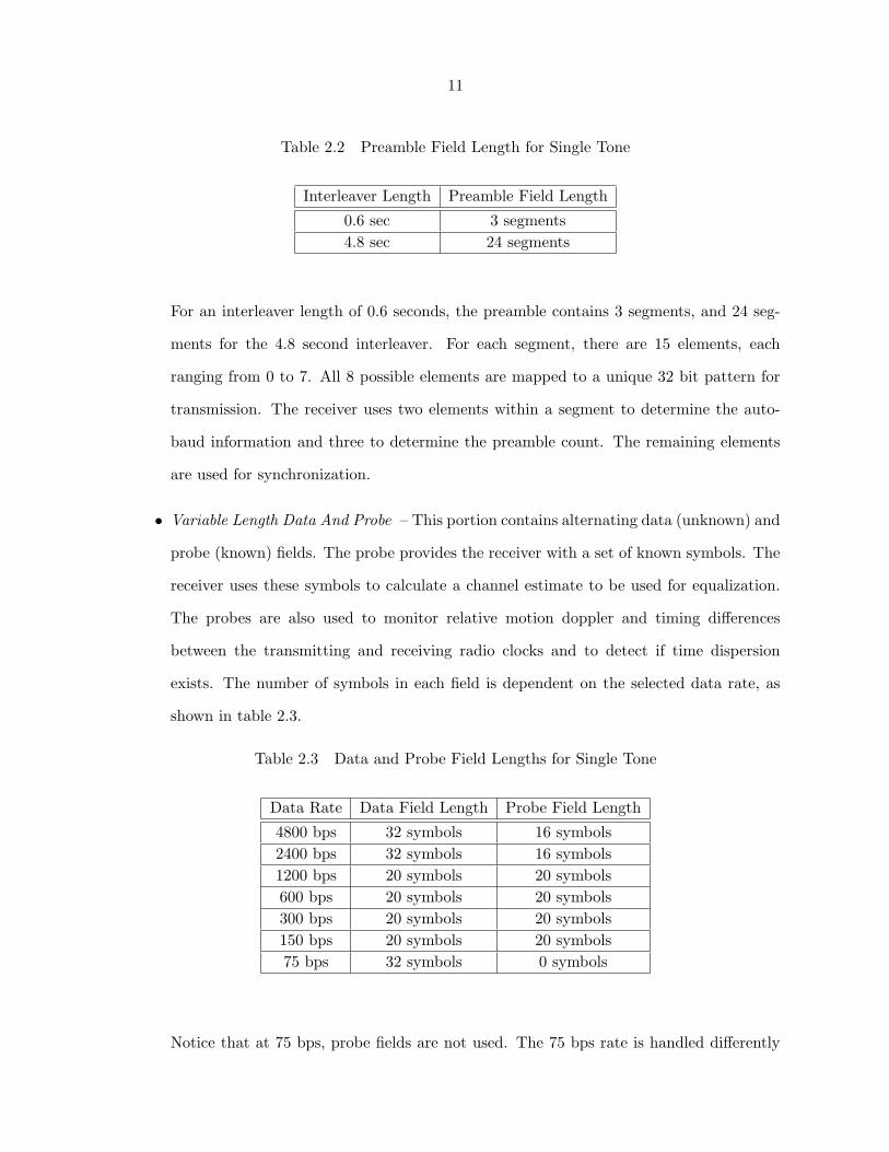
For an interleaver length of 0.6 seconds, the preamble contains 3 segments, and 24 seg-
ments for the 4.8 second interleaver. For each segment, there are 15 elements, each
ranging from 0 to 7. All 8 possible elements are mapped to a unique 32 bit pattern for
transmission. The receiver uses two elements within a segment to determine the auto-
baud information and three to determine the preamble count. The remaining elements
are used for synchronization.
• Variable Length Data And Probe – This portion contains alternating data (unknown) and
probe (known) fields. The probe provides the receiver with a set of known symbols. The
receiver uses these symbols to calculate a channel estimate to be used for equalization.
The probes are also used to monitor relative motion doppler and timing differences
between the transmitting and receiving radio clocks and to detect if time dispersion
exists. The number of symbols in each field is dependent on the selected data rate, as
shown in table 2.3.
Table 2.3 Data and Probe Field Lengths for Single Tone
Data Rate Data Field Length Probe Field Length
4800 bps 32 symbols 16 symbols2400 bps 32 symbols 16 symbols1200 bps 20 symbols 20 symbols600 bps 20 symbols 20 symbols300 bps 20 symbols 20 symbols150 bps 20 symbols 20 symbols75 bps 32 symbols 0 symbols
Notice that at 75 bps, probe fields are not used. The 75 bps rate is handled differently
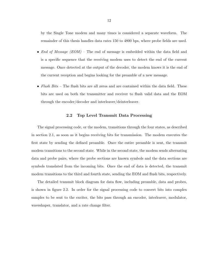
12
by the Single Tone modem and many times is considered a separate waveform. The
remainder of this thesis handles data rates 150 to 4800 bps, where probe fields are used.
• End of Message (EOM) – The end of message is embedded within the data field and
is a specific sequence that the receiving modem uses to detect the end of the current
message. Once detected at the output of the decoder, the modem knows it is the end of
the current reception and begins looking for the preamble of a new message.
• Flush Bits – The flush bits are all zeros and are contained within the data field. These
bits are used on both the transmitter and receiver to flush valid data and the EOM
through the encoder/decoder and interleaver/deinterleaver.
2.2 Top Level Transmit Data Processing
The signal processing code, or the modem, transitions through the four states, as described
in section 2.1, as soon as it begins receiving bits for transmission. The modem executes the
first state by sending the defined preamble. Once the entire preamble is sent, the transmit
modem transitions to the second state. While in the second state, the modem sends alternating
data and probe pairs, where the probe sections are known symbols and the data sections are
symbols translated from the incoming bits. Once the end of data is detected, the transmit
modem transitions to the third and fourth state, sending the EOM and flush bits, respectively.
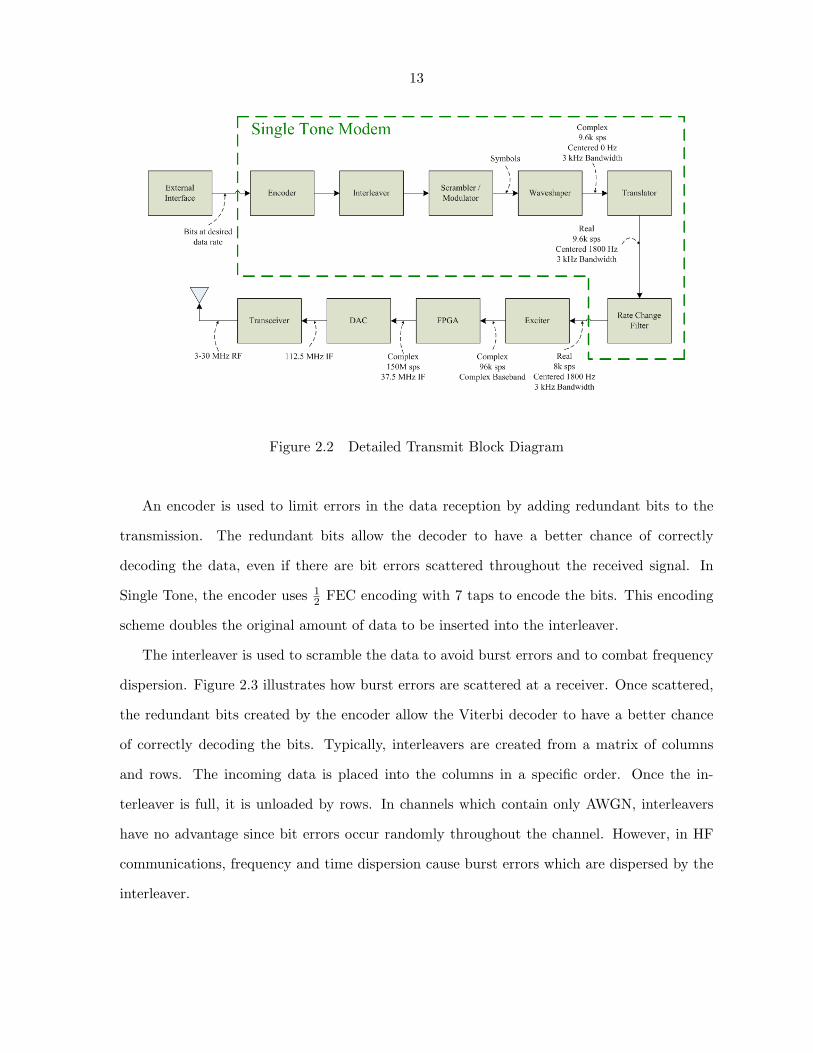
The detailed transmit block diagram for data flow, including preamble, data and probes,
is shown in figure 2.2. In order for the signal processing code to convert bits into complex
samples to be sent to the exciter, the bits pass through an encoder, interleaver, modulator,
waveshaper, translator, and a rate change filter.
13
Figure 2.2 Detailed Transmit Block Diagram
An encoder is used to limit errors in the data reception by adding redundant bits to the
transmission. The redundant bits allow the decoder to have a better chance of correctly
decoding the data, even if there are bit errors scattered throughout the received signal. In
Single Tone, the encoder uses 12 FEC encoding with 7 taps to encode the bits. This encoding
scheme doubles the original amount of data to be inserted into the interleaver.
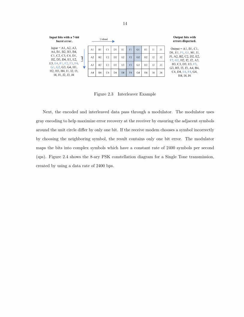
The interleaver is used to scramble the data to avoid burst errors and to combat frequency
dispersion. Figure 2.3 illustrates how burst errors are scattered at a receiver. Once scattered,
the redundant bits created by the encoder allow the Viterbi decoder to have a better chance
of correctly decoding the bits. Typically, interleavers are created from a matrix of columns
and rows. The incoming data is placed into the columns in a specific order. Once the in-
terleaver is full, it is unloaded by rows. In channels which contain only AWGN, interleavers
have no advantage since bit errors occur randomly throughout the channel. However, in HF
communications, frequency and time dispersion cause burst errors which are dispersed by the
interleaver.
14
Figure 2.3 Interleaver Example
Next, the encoded and interleaved data pass through a modulator. The modulator uses
gray encoding to help maximize error recovery at the receiver by ensuring the adjacent symbols
around the unit circle differ by only one bit. If the receive modem chooses a symbol incorrectly
by choosing the neighboring symbol, the result contains only one bit error. The modulator
maps the bits into complex symbols which have a constant rate of 2400 symbols per second
(sps). Figure 2.4 shows the 8-ary PSK constellation diagram for a Single Tone transmission,
created by using a data rate of 2400 bps.
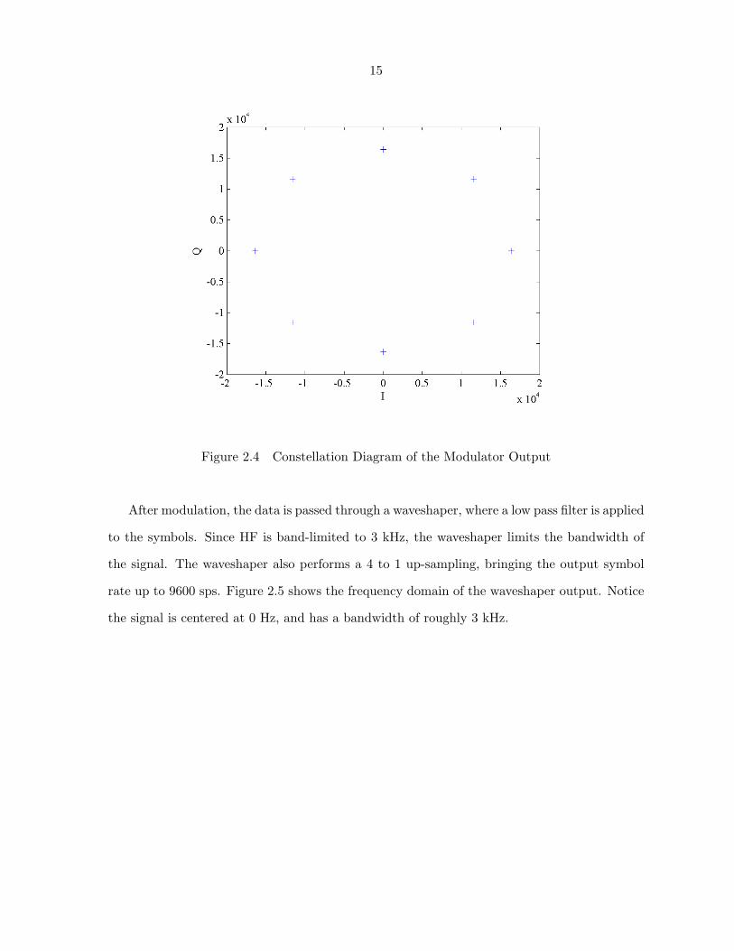
15
Figure 2.4 Constellation Diagram of the Modulator Output
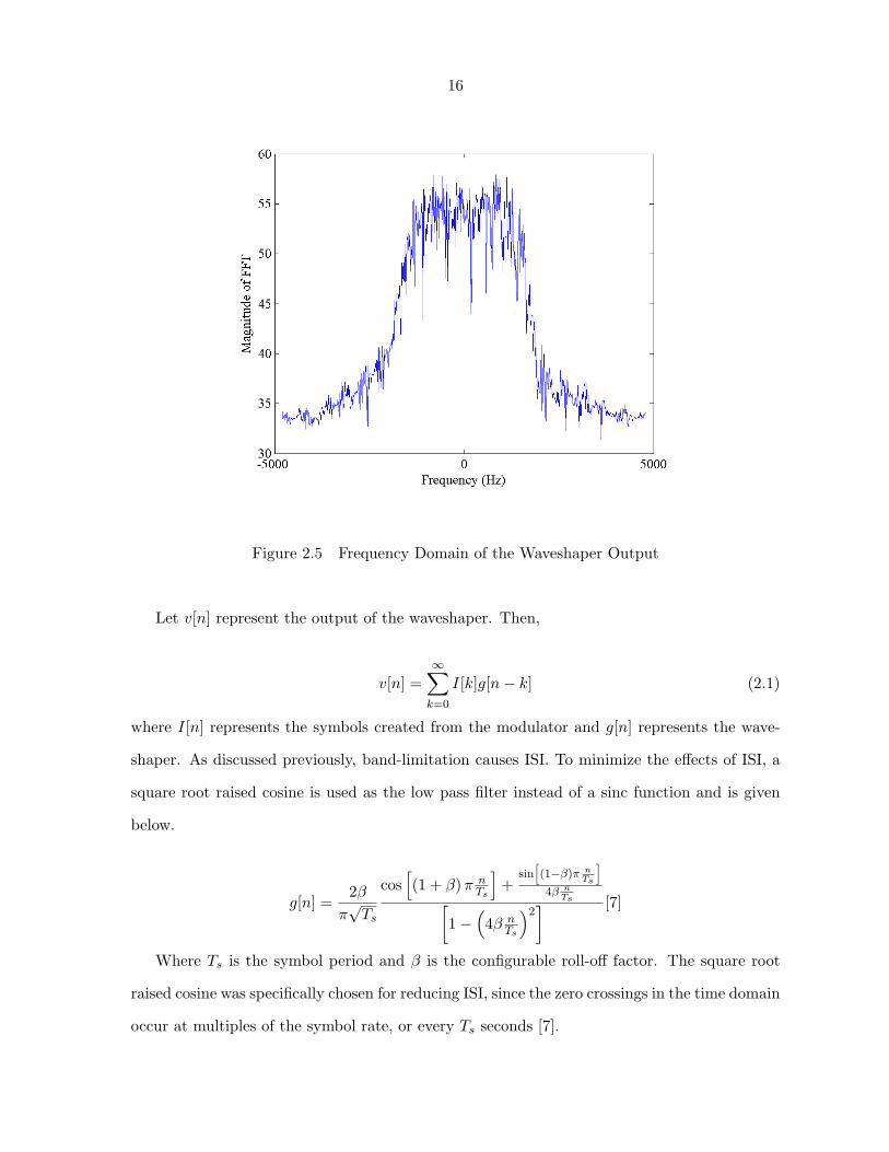
After modulation, the data is passed through a waveshaper, where a low pass filter is applied
to the symbols. Since HF is band-limited to 3 kHz, the waveshaper limits the bandwidth of
the signal. The waveshaper also performs a 4 to 1 up-sampling, bringing the output symbol
rate up to 9600 sps. Figure 2.5 shows the frequency domain of the waveshaper output. Notice
the signal is centered at 0 Hz, and has a bandwidth of roughly 3 kHz.
16
Figure 2.5 Frequency Domain of the Waveshaper Output
Let v[n] represent the output of the waveshaper. Then,
v[n] =∞∑k=0
I[k]g[n− k] (2.1)
where I[n] represents the symbols created from the modulator and g[n] represents the wave-
shaper. As discussed previously, band-limitation causes ISI. To minimize the effects of ISI, a
square root raised cosine is used as the low pass filter instead of a sinc function and is given
below.
g[n] =2β
π√Ts
cos[(1 + β)π n
Ts
]+
sin[(1−β)π n
Ts
]4β n
Ts[1−
(4β n
Ts
)2] [7]
Where Ts is the symbol period and β is the configurable roll-off factor. The square root
raised cosine was specifically chosen for reducing ISI, since the zero crossings in the time domain
occur at multiples of the symbol rate, or every Ts seconds [7].
17
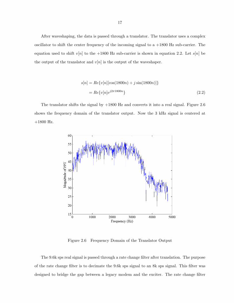
After waveshaping, the data is passed through a translator. The translator uses a complex
oscillator to shift the center frequency of the incoming signal to a +1800 Hz sub-carrier. The
equation used to shift v[n] to the +1800 Hz sub-carrier is shown in equation 2.2. Let s[n] be
the output of the translator and v[n] is the output of the waveshaper.
s[n] = Re{v[n][cos(1800n) + j sin(1800n)]}
= Re{v[n]ej2π1800n} (2.2)
The translator shifts the signal by +1800 Hz and converts it into a real signal. Figure 2.6
shows the frequency domain of the translator output. Now the 3 kHz signal is centered at
+1800 Hz.
Figure 2.6 Frequency Domain of the Translator Output
The 9.6k sps real signal is passed through a rate change filter after translation. The purpose
of the rate change filter is to decimate the 9.6k sps signal to an 8k sps signal. This filter was
designed to bridge the gap between a legacy modem and the exciter. The rate change filter
18
is implemented as a polyphase filter which interpolates the 9.6k sps signal to 96k sps, then
decimates to 8k sps. The output of the rate change filter is a real 8k sps audio signal.
The rate change filter is the final block of the Single Tone modem software. The exciter,
field programmable gate array (FPGA), digital to analog converter (DAC), and transceiver
implement additional signal processing functions needed for an HF radio. The exciter has three
major responsibilities: complex bandpass filtering, LSB/USB selection, and interpolation. The
incoming real 8k sps audio signal is first passed through a complex bandpass filter. If LSB,
rather that USB, is desired, the exciter will invert the center frequency of the signal from 1800
to -1800 Hz. The exciter then interpolates the complex signal from 8k sps to 96k sps before
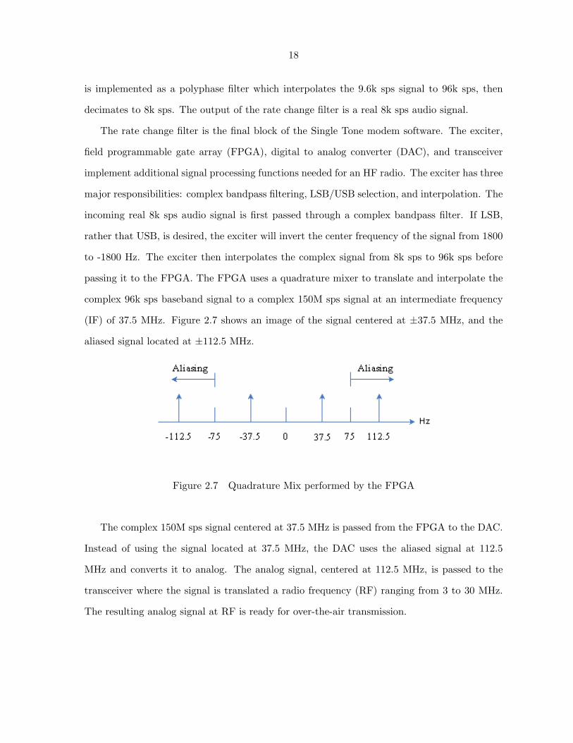
passing it to the FPGA. The FPGA uses a quadrature mixer to translate and interpolate the
complex 96k sps baseband signal to a complex 150M sps signal at an intermediate frequency
(IF) of 37.5 MHz. Figure 2.7 shows an image of the signal centered at ±37.5 MHz, and the
aliased signal located at ±112.5 MHz.
Figure 2.7 Quadrature Mix performed by the FPGA
The complex 150M sps signal centered at 37.5 MHz is passed from the FPGA to the DAC.
Instead of using the signal located at 37.5 MHz, the DAC uses the aliased signal at 112.5
MHz and converts it to analog. The analog signal, centered at 112.5 MHz, is passed to the
transceiver where the signal is translated a radio frequency (RF) ranging from 3 to 30 MHz.
The resulting analog signal at RF is ready for over-the-air transmission.
19
CHAPTER 3. CHANNEL MODEL AND RECEIVE PATH
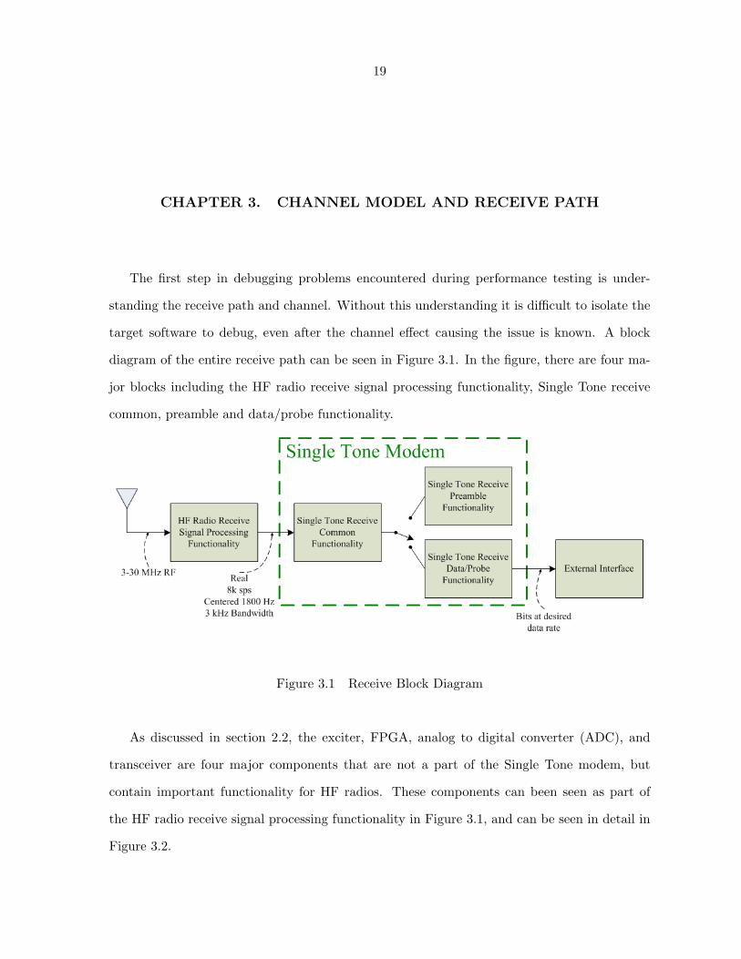
The first step in debugging problems encountered during performance testing is under-
standing the receive path and channel. Without this understanding it is difficult to isolate the
target software to debug, even after the channel effect causing the issue is known. A block
diagram of the entire receive path can be seen in Figure 3.1. In the figure, there are four ma-
jor blocks including the HF radio receive signal processing functionality, Single Tone receive
common, preamble and data/probe functionality.
Figure 3.1 Receive Block Diagram
As discussed in section 2.2, the exciter, FPGA, analog to digital converter (ADC), and
transceiver are four major components that are not a part of the Single Tone modem, but
contain important functionality for HF radios. These components can been seen as part of
the HF radio receive signal processing functionality in Figure 3.1, and can be seen in detail in
Figure 3.2.
20
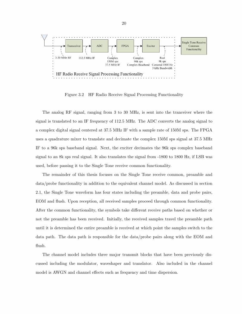
Figure 3.2 HF Radio Receive Signal Processing Functionality
The analog RF signal, ranging from 3 to 30 MHz, is sent into the tranceiver where the
signal is translated to an IF frequency of 112.5 MHz. The ADC converts the analog signal to
a complex digital signal centered at 37.5 MHz IF with a sample rate of 150M sps. The FPGA
uses a quadrature mixer to translate and decimate the complex 150M sps signal at 37.5 MHz
IF to a 96k sps baseband signal. Next, the exciter decimates the 96k sps complex baseband
signal to an 8k sps real signal. It also translates the signal from -1800 to 1800 Hz, if LSB was
used, before passing it to the Single Tone receive common functionality.
The remainder of this thesis focuses on the Single Tone receive common, preamble and
data/probe functionality in addition to the equivalent channel model. As discussed in section
2.1, the Single Tone waveform has four states including the preamble, data and probe pairs,
EOM and flush. Upon reception, all received samples proceed through common functionality.
After the common functionality, the symbols take different receive paths based on whether or
not the preamble has been received. Initially, the received samples travel the preamble path
until it is determined the entire preamble is received at which point the samples switch to the
data path. The data path is responsible for the data/probe pairs along with the EOM and
flush.
The channel model includes three major transmit blocks that have been previously dis-
cussed including the modulator, waveshaper and translator. Also included in the channel
model is AWGN and channel effects such as frequency and time dispersion.
21
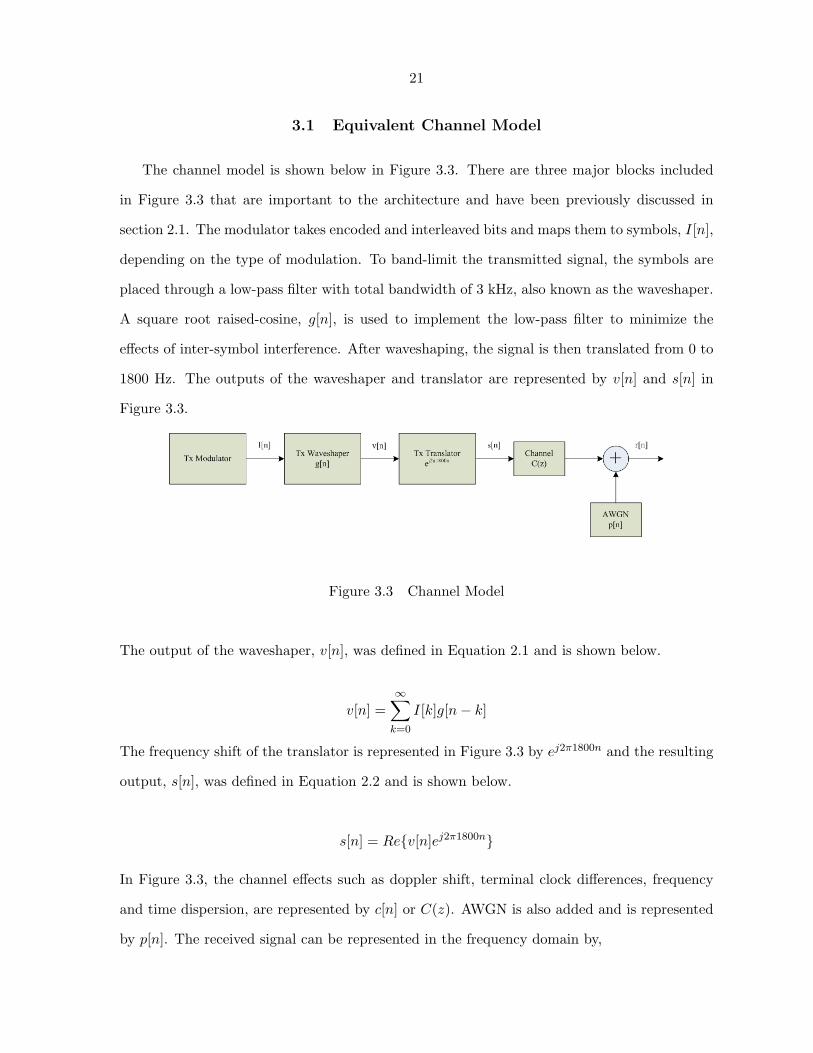
3.1 Equivalent Channel Model
The channel model is shown below in Figure 3.3. There are three major blocks included
in Figure 3.3 that are important to the architecture and have been previously discussed in
section 2.1. The modulator takes encoded and interleaved bits and maps them to symbols, I[n],
depending on the type of modulation. To band-limit the transmitted signal, the symbols are
placed through a low-pass filter with total bandwidth of 3 kHz, also known as the waveshaper.
A square root raised-cosine, g[n], is used to implement the low-pass filter to minimize the
effects of inter-symbol interference. After waveshaping, the signal is then translated from 0 to
1800 Hz. The outputs of the waveshaper and translator are represented by v[n] and s[n] in
Figure 3.3.
Figure 3.3 Channel Model
The output of the waveshaper, v[n], was defined in Equation 2.1 and is shown below.
v[n] =∞∑k=0
I[k]g[n− k]
The frequency shift of the translator is represented in Figure 3.3 by ej2π1800n and the resulting
output, s[n], was defined in Equation 2.2 and is shown below.
s[n] = Re{v[n]ej2π1800n}
In Figure 3.3, the channel effects such as doppler shift, terminal clock differences, frequency
and time dispersion, are represented by c[n] or C(z). AWGN is also added and is represented
by p[n]. The received signal can be represented in the frequency domain by,
22
R(z) = S(z)C(z) + P (z)
or in the time domain,
r[n] = s[n]⊗ c[n] + p[n]
=∞∑
k=−∞s[k]c[n− k] + p[n]
Where ⊗ represents the convolution of two signals.
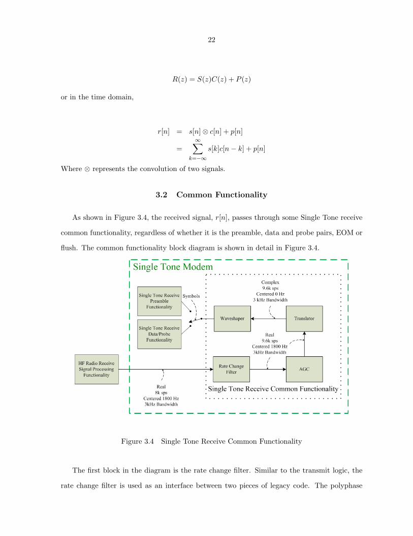
3.2 Common Functionality
As shown in Figure 3.4, the received signal, r[n], passes through some Single Tone receive
common functionality, regardless of whether it is the preamble, data and probe pairs, EOM or
flush. The common functionality block diagram is shown in detail in Figure 3.4.
Figure 3.4 Single Tone Receive Common Functionality
The first block in the diagram is the rate change filter. Similar to the transmit logic, the
rate change filter is used as an interface between two pieces of legacy code. The polyphase
23
filter interpolates the 8k real signal to 96k sps before decimating down to 9.6k sps. The output
of the rate change filter is then passed to the automatic gain control (AGC).
The AGC is a control loop which uses the output signal level strength to vary the gain on
the input signal. It smoothes the amplitude envelope to avoid drastic changes in signal level,
and maximizes dynamic range. After the AGC, the received signal is shifted by the translator.
Similar to the transmit functionality, a complex oscillator is used to translate the real signal
at 1800 Hz to a complex signal at 0 Hz. The 3 kHz bandwidth of the signal remains unchanged.
The output of the translator is then passed to the waveshaper.
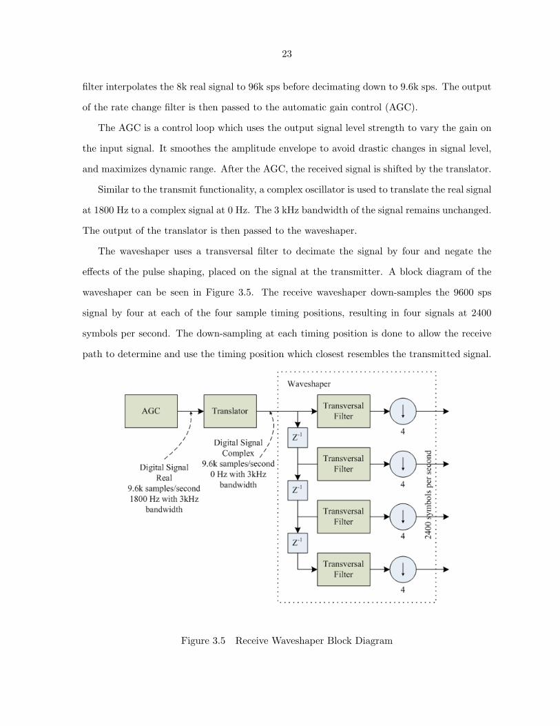
The waveshaper uses a transversal filter to decimate the signal by four and negate the
effects of the pulse shaping, placed on the signal at the transmitter. A block diagram of the
waveshaper can be seen in Figure 3.5. The receive waveshaper down-samples the 9600 sps
signal by four at each of the four sample timing positions, resulting in four signals at 2400
symbols per second. The down-sampling at each timing position is done to allow the receive
path to determine and use the timing position which closest resembles the transmitted signal.
Figure 3.5 Receive Waveshaper Block Diagram
24
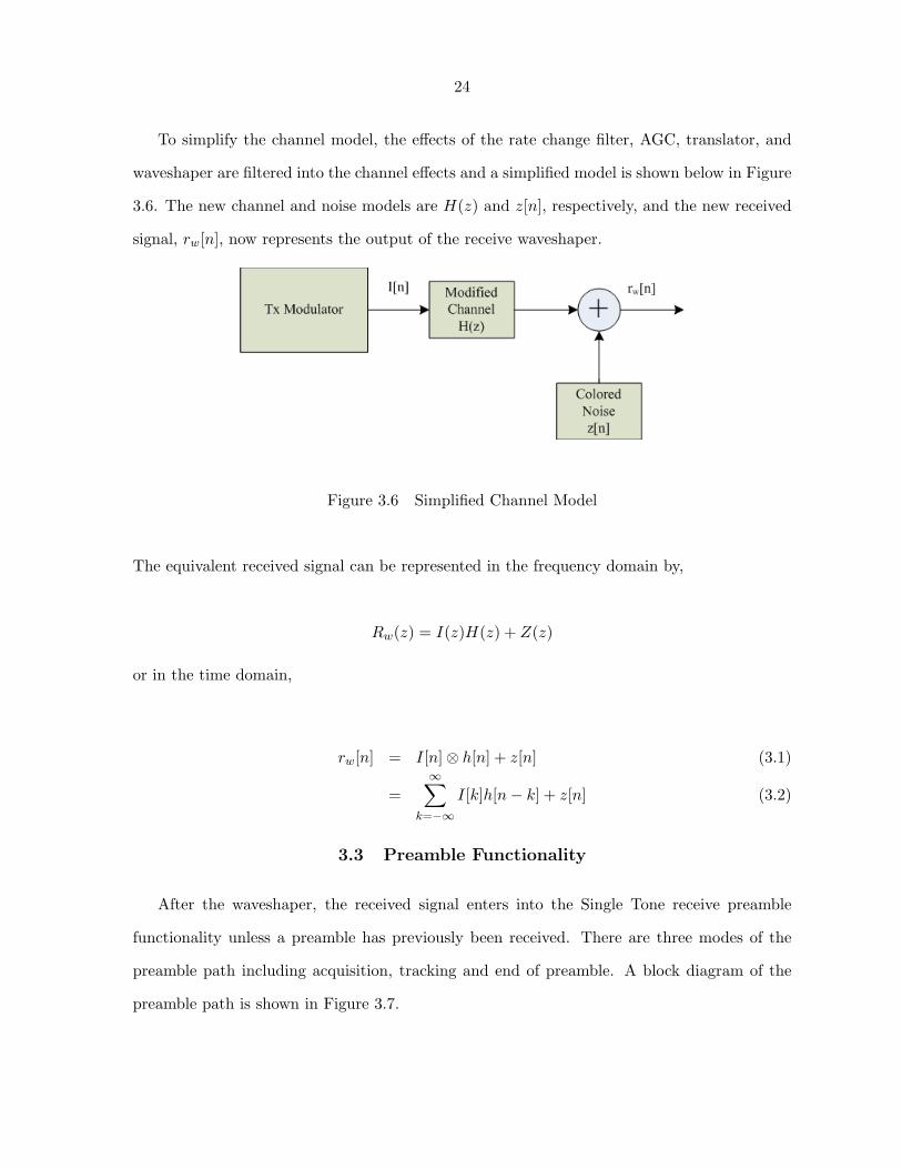
To simplify the channel model, the effects of the rate change filter, AGC, translator, and
waveshaper are filtered into the channel effects and a simplified model is shown below in Figure
3.6. The new channel and noise models are H(z) and z[n], respectively, and the new received
signal, rw[n], now represents the output of the receive waveshaper.
Figure 3.6 Simplified Channel Model
The equivalent received signal can be represented in the frequency domain by,
Rw(z) = I(z)H(z) + Z(z)
or in the time domain,
rw[n] = I[n]⊗ h[n] + z[n] (3.1)
=∞∑
k=−∞I[k]h[n− k] + z[n] (3.2)
3.3 Preamble Functionality
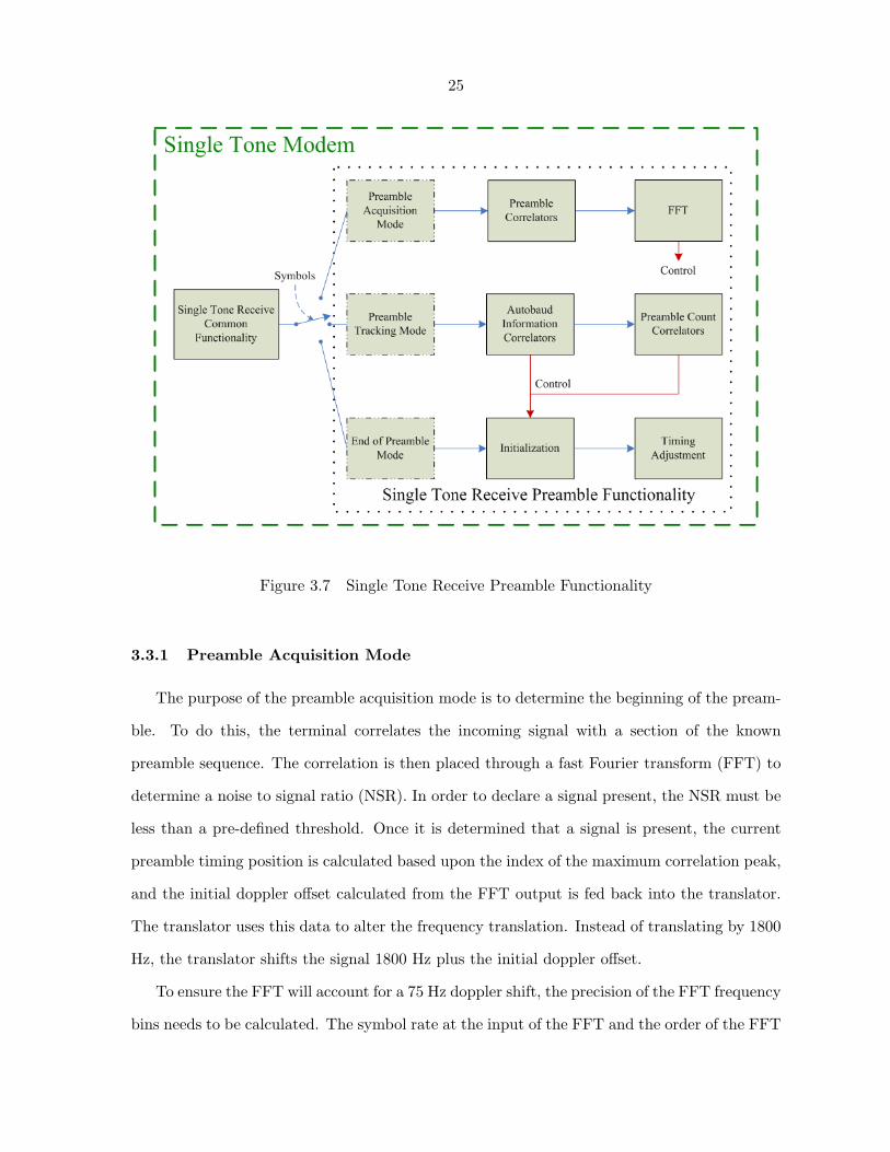
After the waveshaper, the received signal enters into the Single Tone receive preamble
functionality unless a preamble has previously been received. There are three modes of the
preamble path including acquisition, tracking and end of preamble. A block diagram of the
preamble path is shown in Figure 3.7.
25
Figure 3.7 Single Tone Receive Preamble Functionality
3.3.1 Preamble Acquisition Mode
The purpose of the preamble acquisition mode is to determine the beginning of the pream-
ble. To do this, the terminal correlates the incoming signal with a section of the known
preamble sequence. The correlation is then placed through a fast Fourier transform (FFT) to
determine a noise to signal ratio (NSR). In order to declare a signal present, the NSR must be
less than a pre-defined threshold. Once it is determined that a signal is present, the current
preamble timing position is calculated based upon the index of the maximum correlation peak,
and the initial doppler offset calculated from the FFT output is fed back into the translator.
The translator uses this data to alter the frequency translation. Instead of translating by 1800
Hz, the translator shifts the signal 1800 Hz plus the initial doppler offset.
To ensure the FFT will account for a 75 Hz doppler shift, the precision of the FFT frequency
bins needs to be calculated. The symbol rate at the input of the FFT and the order of the FFT
26
will determine the frequency bin precision. Assume the input symbol rate is 2400 symbols per
second and that the FFT order is 256, then the precision of the output frequency bins would
be 2400256 = 9.375 Hz. The FFT output bins would cover a dynamic range of −1190.625 Hz
to 1200 Hz. A 256 point FFT would be very processor intensive to execute, and since the
military standard only requires the single tone modem to cover a dynamic range of −75 Hz
to 75 Hz, only 19 of the 256 bins would be used. By using 19 bins, the doppler estimate
would have a dynamic range of −84.375 Hz to 84.375 with precision of 9.375 Hz. By taking a
smaller FFT, the computation complexity would be drastically reduced, but the frequency bin
precision drastically decreases. If a 16-point FFT is performed on the 2400 symbols per second
signal, the resulting frequency bin precision would be 240016 = 150 Hz. To compensate for this
precision loss, a method of down-sampling can be performed prior to the FFT. Assume the
new input symbol rate to the FFT is 300 symbols per second, then the frequency bin precision
of the 16-point FFT becomes 30016 = 18.75 Hz and the dynamic range covered would be −131.25
Hz to 150 Hz. By using 11 of the 16 bins, the doppler estimate would have a dynamic range
of −93.75 Hz to 93.75 with a precision of 18.75 Hz.
As discussed in section 2.1, the variable length preamble consists of 3 to 24 segments
depending on the interleaver length. Assuming the initial correlation detects the first segment,
2 to 23 preamble segments will be received after the end of the current segment. These
additional preamble segments can be used to avoid false acquisition. From the initial correlation
and FFT, the timing position within the preamble segment is calculated. The terminal can use
the timing position and the knowledge of the preamble to predict the number of correlations
before the NSR will again dip below the threshold. If the next correlation which slides below
the threshold matches the predicted, the preamble is declared as detected. After detection,
the terminal transitions to the preamble tracking mode.
3.3.2 Preamble Tracking Mode
The preamble tracking mode determines the preamble count and autobaud information
from the preamble. Once the preamble count is determined, this mode also keeps track of the
27
number of remaining preamble segments. As discussed in section 2.1, 2 of the 15 elements
within a preamble segment contain the autobaud information and 3 of the 15 elements contain
the preamble count. The preamble count indicates the number of preamble segments remaining
before the end of the preamble.
The terminal uses the preamble timing position, determined during the preamble acquisi-
tion mode, to calculate the location of the two elements containing the autobaud information
in the current preamble segment. To determine the autobaud information, a correlation be-
tween these elements and all possible options is completed. The option, from which the largest
correlation peak is produced, is determined to be the correct data rate and interleaver length.
Like the preamble acquisition mode, a method is used to minimize the possibility of error
while detecting the autobaud information. These correlations are executed over each of the
remaining preamble segments. The correlators increment a counter pertaining to the data rate
and interleaver length detected in the current segment. At the end of the preamble, the option
which produced the most maximum correlations is used to assign the data rate and interleaver
length. This method allows for some receive errors and false positives to occur but is still able
to choose the correct autobaud information.
Another correlation is performed at the three elements containing the preamble count in-
formation. Again, the option from which the largest correlation peak is produced is used as
the preamble count value. Since the preamble can vary between 3 and 24 segments, the pream-
ble count contains the number of preamble segments remaining to be received. To minimize
the possibility of errors, this correlation is executed on consecutive preamble segments. If the
preamble count on the next frame is one less than the preamble count on the current frame,
the preamble count has most likely been determined without error.
Once the preamble count has been determined, the terminal continues to track the incoming
preamble segments until the preamble count becomes zero. When the preamble count reaches
zero, the terminal has detected the end of the preamble and transitions to the end of preamble
mode.
28
3.3.3 End of Preamble Mode
During the end of preamble mode, the terminal uses the autobaud information to initialize
the deinterleaver and decoder. Also calculated at this time is an initial channel estimate, using
a least mean square (LMS) algorithm. The known end of the preamble is used along with
the received signal to calculate the initial channel estimate. This channel estimate is used to
initialize the coefficients for the matched filter, feedforward and feedback coefficients for the
zero-forcing decision feedback equalizer (ZF-DFE).
To make calculations easier for the Single Tone receive data functionality, this mode also
performs a timing adjustment. The initial timing position, calculated during initial acquisition,
is used to determine the number of preamble and data samples present in the modem. The
terminal makes an internal timing adjustment to ensure the preamble and data boundary
occurs at a specific location to allow the data path to run more efficiently.
3.4 Data/Probe Functionality
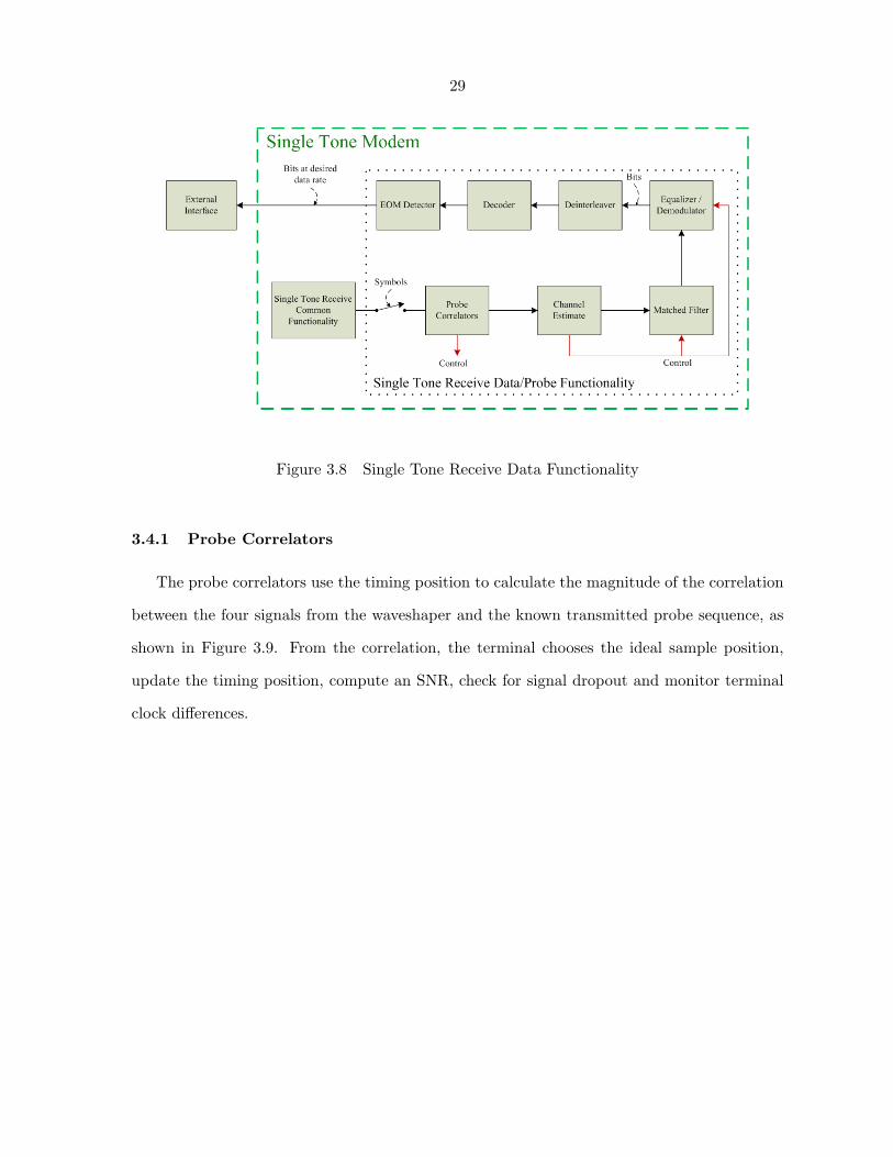
Once the end of the preamble has been determined, rather than entering the Single Tone
receive preamble functionality, the received signal takes the data/probe path after passing
through the waveshaper. As shown in Figure 3.8, the block diagram of the data path in-
cludes a probe correlator, channel estimator, matched filter, an equalizer and demodulator, a
descrambler, deinterleaver, decoder and an EOM detector. After passing through the EOM
detector, the data bits are passed to the external interface.
29
Figure 3.8 Single Tone Receive Data Functionality
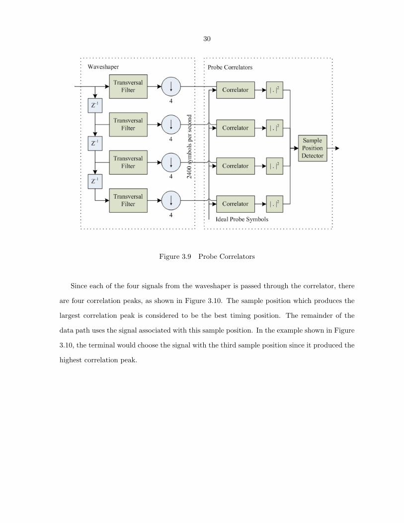
3.4.1 Probe Correlators
The probe correlators use the timing position to calculate the magnitude of the correlation
between the four signals from the waveshaper and the known transmitted probe sequence, as
shown in Figure 3.9. From the correlation, the terminal chooses the ideal sample position,
update the timing position, compute an SNR, check for signal dropout and monitor terminal
clock differences.
30
Figure 3.9 Probe Correlators
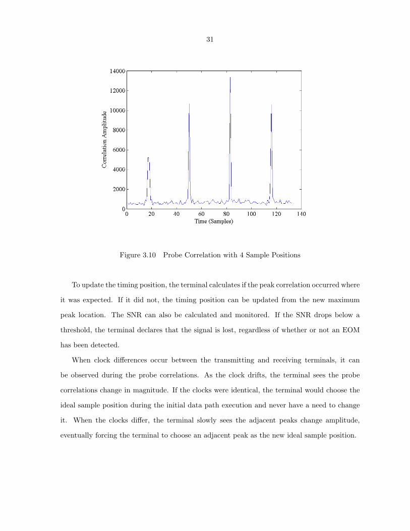
Since each of the four signals from the waveshaper is passed through the correlator, there
are four correlation peaks, as shown in Figure 3.10. The sample position which produces the
largest correlation peak is considered to be the best timing position. The remainder of the
data path uses the signal associated with this sample position. In the example shown in Figure
3.10, the terminal would choose the signal with the third sample position since it produced the
highest correlation peak.
31
Figure 3.10 Probe Correlation with 4 Sample Positions
To update the timing position, the terminal calculates if the peak correlation occurred where
it was expected. If it did not, the timing position can be updated from the new maximum
peak location. The SNR can also be calculated and monitored. If the SNR drops below a
threshold, the terminal declares that the signal is lost, regardless of whether or not an EOM
has been detected.
When clock differences occur between the transmitting and receiving terminals, it can
be observed during the probe correlations. As the clock drifts, the terminal sees the probe
correlations change in magnitude. If the clocks were identical, the terminal would choose the
ideal sample position during the initial data path execution and never have a need to change
it. When the clocks differ, the terminal slowly sees the adjacent peaks change amplitude,
eventually forcing the terminal to choose an adjacent peak as the new ideal sample position.
32
3.4.2 Channel Estimate
From Equation 3.2, the received signal is rw[n] =∑∞
k=−∞ I[k]h[n− k] + z[n]. The purpose
of the receiving terminal is to estimate the transmitted symbol, I[n]. In order to estimate I[n],
an estimate of the channel effects, h[n], needs to be calculated. One method that can be used
to estimate h[n] is the LMS algorithm.
3.4.2.1 LMS Algorithm
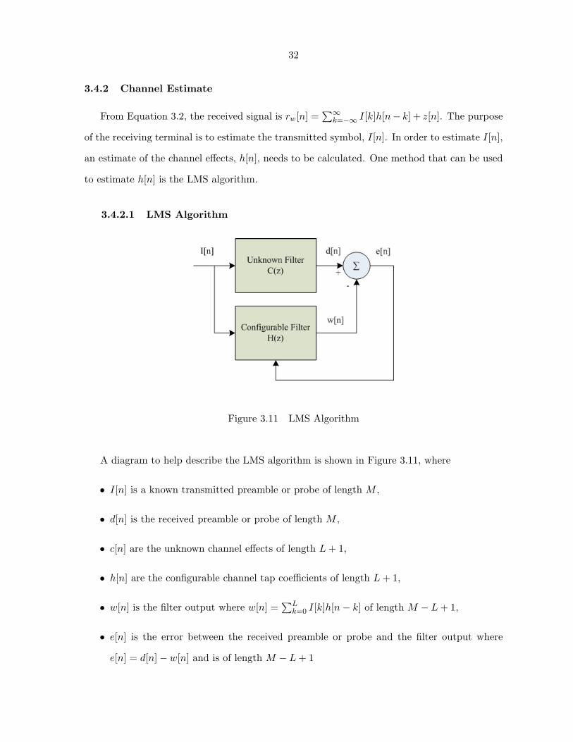
Figure 3.11 LMS Algorithm
A diagram to help describe the LMS algorithm is shown in Figure 3.11, where
• I[n] is a known transmitted preamble or probe of length M ,
• d[n] is the received preamble or probe of length M ,
• c[n] are the unknown channel effects of length L+ 1,
• h[n] are the configurable channel tap coefficients of length L+ 1,
• w[n] is the filter output where w[n] =∑L
k=0 I[k]h[n− k] of length M − L+ 1,
• e[n] is the error between the received preamble or probe and the filter output where
e[n] = d[n]− w[n] and is of length M − L+ 1
33
The LMS algorithm initializes the tap coefficients, h[n], to an initial value. The output
of the filter and error are estimated and are used to update the new tap coefficients. Multi-
ple iterations minimize the error, e[n], and produce a known filter that closely resembles an
unknown filter, C(z). The steps to the LMS algorithm are shown below.
• Initialize filter coefficients, h, to zero
• Calculate all M − L+ 1 w[n]s where, w[n] =∑L
k=0 I[k]h[n− k]
• Calculate all M − L+ 1 e[n]s where, e[n] = d[n]− w[n]
• Calculate all L+ 1 hnews where,
hnew[n] = h[n]− 12B
[d
dh
[E(|e[n]|2
)]]= h[n]− 1
2B
[2E(d
dh
[|e[n]|2
])]= h[n]−B
[E
(d
dh
[|e[n]|2
])]= h[n]−B
[E
(d
dh[e[n]e[n]∗]
)]= h[n] +B [I[n]e[n]∗]
• Repeat all steps except the first initialization step
Once the L+ 1 taps of the channel estimate have been estimated, rw[n] from Equation 3.2
can be rewritten as,
rw[n] =L∑k=0
I[k]h[n− k] + z[n]
3.4.3 Matched Filter, Equalizer, and Demodulator
The first two blocks of the data path, the probe correlator and the channel estimator,
produce control data by comparing the received signal with known probe data. The control
data from the channel estimate is used to configure the matched filter, feedforward and feedback
coefficients of the ZF-DFE.
34
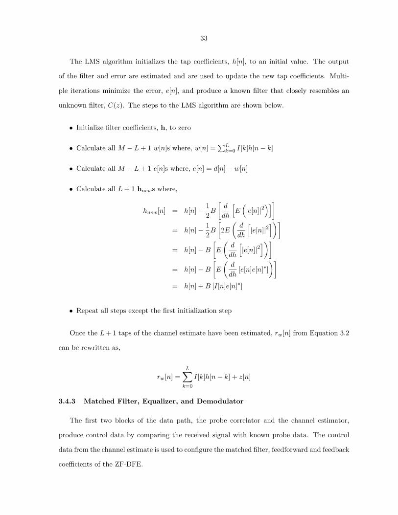
3.4.3.1 Matched Filter
According to Proakis [5], the optimal demodulator can be realized as a matched filter to
the channel estimate, h[n], having impulse response h∗[−n] [5], as shown in Figure 3.12.
Figure 3.12 Matched Filter at the Receiver
Using Equation 3.1 where rw[n] = I[n]⊗h[n] + z[n], the output of the matched filter, y[n], can
be defined as,
y[n] = rw[n]⊗ h∗[−n]
= (I[n]⊗ h[n] + z[n])⊗ h∗[−n]
= I[n]⊗ h[n]⊗ h∗[−n] + z[n]⊗ h∗[−n] (3.3)
Let x[n] = h[n] ⊗ h∗[−n], where h[n] has non-zero values from 0 ≤ n ≤ L and h∗[−n] has
non-zero values from −L ≤ n ≤ 0. Then x[n] has non-zero values from −L ≤ n ≤ L, and
x[n] =L∑k=0
h∗[−k]h[n− k] (3.4)
Then Equation 3.3 can be simplified to
y[n] = I[n]⊗ x[n] + z[n]⊗ h∗[−n] (3.5)
=L∑
k=−LI[k]x[n− k] +
0∑k=−L
z[k]h∗[−n− k]
=−1∑
k=−LI[k]x[n− k] + I[n]x[0] +
L∑k=1
I[k]x[n− k] +0∑
k=−Lz[k]h∗[−n− k]
The I[n]x[0] term is the desired symbol at the nth sample, the terms∑−1
k=−L I[k]x[n− k] and∑Lk=1 I[k]x[n− k] represent ISI and
∑0k=−L z[k]h∗[−n− k] is colored noise.
35
3.4.3.2 Zero-Forcing Decision Feedback Equalizer
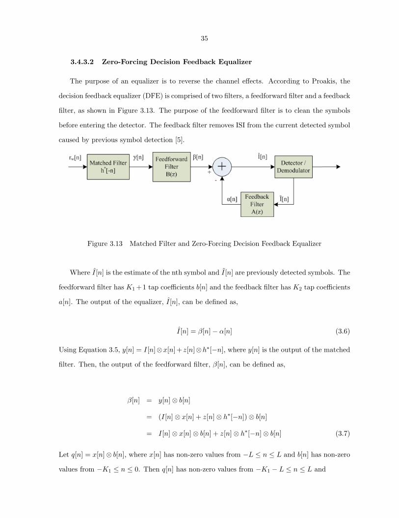
The purpose of an equalizer is to reverse the channel effects. According to Proakis, the
decision feedback equalizer (DFE) is comprised of two filters, a feedforward filter and a feedback
filter, as shown in Figure 3.13. The purpose of the feedforward filter is to clean the symbols
before entering the detector. The feedback filter removes ISI from the current detected symbol
caused by previous symbol detection [5].
Figure 3.13 Matched Filter and Zero-Forcing Decision Feedback Equalizer
Where I[n] is the estimate of the nth symbol and I[n] are previously detected symbols. The
feedforward filter has K1 +1 tap coefficients b[n] and the feedback filter has K2 tap coefficients
a[n]. The output of the equalizer, I[n], can be defined as,
I[n] = β[n]− α[n] (3.6)
Using Equation 3.5, y[n] = I[n]⊗x[n] + z[n]⊗h∗[−n], where y[n] is the output of the matched
filter. Then, the output of the feedforward filter, β[n], can be defined as,
β[n] = y[n]⊗ b[n]
= (I[n]⊗ x[n] + z[n]⊗ h∗[−n])⊗ b[n]
= I[n]⊗ x[n]⊗ b[n] + z[n]⊗ h∗[−n]⊗ b[n] (3.7)
Let q[n] = x[n]⊗ b[n], where x[n] has non-zero values from −L ≤ n ≤ L and b[n] has non-zero
values from −K1 ≤ n ≤ 0. Then q[n] has non-zero values from −K1 − L ≤ n ≤ L and
36
q[n] =0∑
k=−K1
x[k]b[n− k] (3.8)
Then the output of the feedforward filter, can be simplified using the definition of q[n] and
Equation 3.7.
β[n] = I[n]⊗ q[n] + z[n]⊗ h∗[−n]⊗ b[n]
=L∑
k=−L−K1
I[k]q[n− k] + z[n]⊗ h∗[−n]⊗ b[n]
=−1∑
k=−L−K1
I[k]q[n− k] + I[n]q[0] +L∑k=1
I[k]q[n− k] + z[n]⊗ h∗[−n]⊗ b[n] (3.9)
The I[n]q[0] term is the desired symbol at the nth sample, the terms∑−1
k=−L−K1I[k]q[n − k]
and∑L
k=1 I[k]q[n − k] represent ISI and z[n] ⊗ h∗[−n] ⊗ b[n] is colored noise. Now Equation
3.6, or the output of the equalizer, can be expanded using Equation 3.9.
I[n] = I[n]q[0] +−1∑
k=−L−K1
I[k]q[n− k] +L∑k=1
I[k]q[n− k] + z[n]⊗ h∗[−n]⊗ b[n]− α[n] (3.10)
The output of the feedback filter, α[n], can be defined as,
α[n] = I[n]⊗ a[n]
=K2∑k=1
I[k]a[n− k] (3.11)
Then the output of the equalizer can be expanded further using the output of the feedback
filter, Equation 3.11, and Equation 3.10.
I[n] = I[n]q[0] +−1∑
k=−L−K1
I[k]q[n− k] +L∑k=1
I[k]q[n− k] + z[n]⊗ h∗[−n]⊗ b[n]
−K2∑k=1
I[k]a[n− k] (3.12)
37
The purpose of a zero-forcing equalizer is to minimize the effects of ISI. To do this, the feedfor-
ward and feedback coefficients need to be initialized using certain conditions. Assume K2 ≤ L
then Equation 3.12 can be expanded as,
I[n] =−1∑
k=−L−K1
I[k]q[n− k] + I[n]q[0] +K2∑k=1
I[k]q[n− k] +L∑
k=K2+1
I[k]q[n− k]
+ z[n]⊗ h∗[−n]⊗ b[n]−K2∑k=1
I[k]a[n− k] +
[K2∑k=1
I[k]q[n− k]−K2∑k=1
I[k]q[n− k]
]
=−1∑
k=−L−K1
I[k]q[n− k] + I[n]q[0] +L∑
k=K2+1
I[k]q[n− k] + z[n]⊗ h∗[−n]⊗ b[n]
+K2∑k=1
(I[k]− I[k]
)q[n− k]−
K2∑k=1
I[k] (q[n− k]− a[n− k]) (3.13)
Assume that the detector is making good decisions, such that I[n] = I[n], and assign the K2
feedback coefficients, a[n], to
a[n] = q[n] (3.14)
where q[n] is defined in Equation 3.8, then Equation 3.13 can be reduced to,
I[n] =−1∑
k=−L−K1
I[k]q[n− k] + I[n]q[0] +L∑
k=K2+1
I[k]q[n− k] + z[n]⊗ h∗[−n]⊗ b[n]
The ISI is reduced to∑−1
k=−L−K1I[k]q[n−k] and
∑Lk=K2+1 I[k]q[n−k]. To completely eliminate
the ISI, the feedforward coefficients need to be assigned such that,
q[n] =
1 for n = 0
0 for −L−K1 ≤ n ≤ −1 and K2 + 1 ≤ n ≤ L
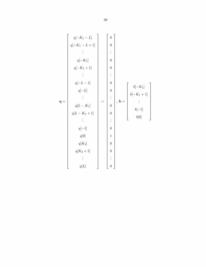
Assume that K1 ≥ L and define the following vectors and matrices,
38
q =
q[−K1 − L]
q[−K1 − L+ 1]...
q[−K1]
q[−K1 + 1]...
q[−L− 1]
q[−L]...
q[L−K1]
q[L−K1 + 1]...
q[−1]
q[0]
q[K2]
q[K2 + 1]...
q[L]
=
0
0...
0
0...
0
0...
0
0...
0
1
0
0...
0
, b =
b[−K1]
b[−K1 + 1]...
b[−1]
b[0]
39
X =
x[−L] x[−L− 1] · · · x[−L−K1 + 1] x[−L−K1]
x[−L+ 1] x[−L] · · · x[−L−K1 + 2] x[−L−K1 + 1]...
.... . .
......
x[0] x[−1] · · · x[−K1 + 1] x[−K1]
x[1] x[0] · · · x[−K1 + 2] x[−K1 + 1]...
.... . .
......
x[K1 − L− 1] x[K1 − L− 2] · · · x[−L] x[−L− 1]
x[K1 − L] x[K1 − L− 1] · · · x[−L+ 1] x[−L]...
.... . .
......
x[L] x[L− 1] · · · x[L+ 1−K1] x[L−K1]
x[L+ 1] x[L] · · · x[L+ 2−K1] x[L+ 1−K1]...
.... . .
......
x[K1 − 1] x[K1 − 2] · · · x[0] x[−1]
x[K1] x[K1 − 1] · · · x[1] x[0]
x[K2 +K1] x[K2 +K1 − 1] · · · x[K2 + 1] x[K2]
x[K2 +K1 + 1] x[K2 +K1] · · · x[K2 + 2] x[K2 + 1]...
.... . .
......
x[K1 + L] x[K1 + L− 1] · · · x[L+ 1] x[L]
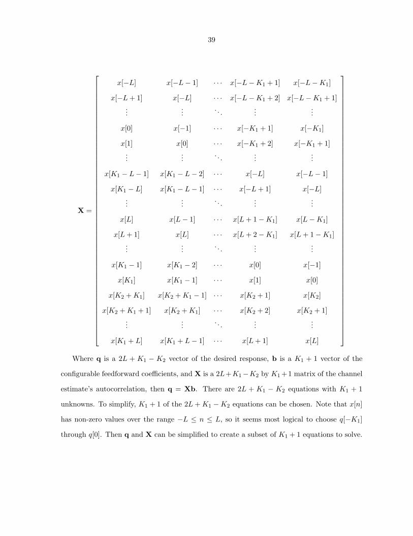
Where q is a 2L + K1 − K2 vector of the desired response, b is a K1 + 1 vector of the
configurable feedforward coefficients, and X is a 2L+K1−K2 by K1 +1 matrix of the channel
estimate’s autocorrelation, then q = Xb. There are 2L + K1 − K2 equations with K1 + 1
unknowns. To simplify, K1 + 1 of the 2L+K1 −K2 equations can be chosen. Note that x[n]
has non-zero values over the range −L ≤ n ≤ L, so it seems most logical to choose q[−K1]
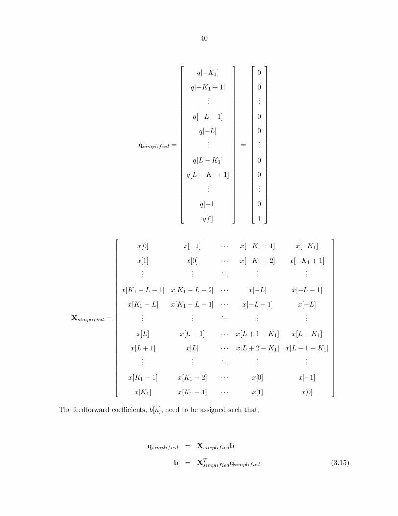
through q[0]. Then q and X can be simplified to create a subset of K1 + 1 equations to solve.
40
qsimplified =
q[−K1]
q[−K1 + 1]...
q[−L− 1]
q[−L]...
q[L−K1]
q[L−K1 + 1]...
q[−1]
q[0]
=
0
0...
0
0...
0
0...
0
1
Xsimplified =
x[0] x[−1] · · · x[−K1 + 1] x[−K1]
x[1] x[0] · · · x[−K1 + 2] x[−K1 + 1]...
.... . .
......
x[K1 − L− 1] x[K1 − L− 2] · · · x[−L] x[−L− 1]
x[K1 − L] x[K1 − L− 1] · · · x[−L+ 1] x[−L]...
.... . .
......
x[L] x[L− 1] · · · x[L+ 1−K1] x[L−K1]
x[L+ 1] x[L] · · · x[L+ 2−K1] x[L+ 1−K1]...
.... . .
......
x[K1 − 1] x[K1 − 2] · · · x[0] x[−1]
x[K1] x[K1 − 1] · · · x[1] x[0]
The feedforward coefficients, b[n], need to be assigned such that,
qsimplified = Xsimplifiedb
b = XTsimplifiedqsimplified (3.15)
41
To minimize processing, the LMS algorithm could be used to initialize the feedforward coef-
ficients where b would be the configurable tap coefficients, X would be the ideal input, and
q would be the desired response. The implementation discussed above documents the current
implementation, but can be improved.
3.4.3.3 Detector / Demodulator
The detector receives the equalized symbol, I[n], and compares it with the ideal constel-
lation diagram. The ideal symbol which minimizes the Euclidean distance to the equalized
symbol is selected as the detected symbol, I[n]. This detected symbol is then used in the
feedback loop of the ZF-DFE, as I[n].
Opposite of the modulator, the demodulator translates the detected symbols into soft
decisions. If the decoder incorrectly chooses the detected symbol, the gray decoding minimizes
bit errors by having neighboring symbols on the constellation diagram differ by one bit. The
soft decisions are then passed to the deinterleaver.
3.4.4 Deinterleaver, Decoder, and EOM Detector
The deinterleaver performs the opposite operation of the interleaver. It descrambles the
received data bits, scattering burst errors across multiple code words to make it possible for
the decoder to correct the errors. Similar to the interleaver, the incoming data bits are placed
into columns in a specific order. Once the deinterleaver is full, the bits are unloaded by rows.
After deinterleaving, the bits are passed to the decoder.
A viterbi decoder is used to decode the FEC encoded data bits. The decoded data bits from
the viterbi decoder are passed to the EOM detector. The EOM detector performs a correlation
between the bits from the decoder and the known EOM sequence. If the resulting correlation
peak is larger than or equal to the EOM detection threshold, the EOM has been detected.
Typically the EOM threshold is set such that no bit errors are allowed in the received EOM.
If the EOM is not successfully detected, the terminal eventually detects a signal loss when the
probe correlators see the SNR drop below a threshold.
42
CHAPTER 4. ISOLATION OF THE SOFTWARE DEFECT USING BIT
ERROR TIMING AND CHANNEL EFFECTS
After the channel model and receive path are understood, the next step in debugging the
Single Tone modem is isolating the software defect. By using the timing of bit errors, and
applying channel effects individually, the debugging efforts can be focused to a certain area
of software. The timing of bit errors can reveal a lot about the location of the problem. Bit
errors which occur at the beginning of the reception indicate a different software defect, than
bit errors occurring at the end. If bit errors occur during the middle of the reception, typically
more information needs to be obtained to further determine the area of software to debug. To
obtain more information, channel effects are applied individually to allow the software defects
associated with each channel effect to be isolated and debugged.
4.1 Software Isolation using Bit Error Timing
Bit errors which occur during testing, may have a repeatable timing pattern that may help
to isolate the software issue. Each bit error position leads to a different section of code to help
begin the debugging process.
4.1.1 Errors at the Beginning of the Reception
If bit errors occur at the beginning of the reception, the area of code to begin debugging
is the preamble path. As discussed in Section 3.3, there are three modes of the preamble path
including acquisition, tracking and end of preamble detection. Bit errors at the beginning of
the reception indicate that the preamble path is the source of the defect, but does not give
enough information to positively determine in which preamble path mode the issue occurs.
43
Preamble Path - Preamble Acquisition Mode: Preamble Correlators
As discussed in Section 3.3.1, the main purpose of the preamble acquisition mode is to
detect the preamble, and calculate initial timing position and doppler shift. The terminal
typically has a method in place within the preamble correlators to avoid false detection. The
method previously discussed uses the maximum correlation from two consecutive preamble
segments and the timing between them to avoid false detection. This method helps to avoid
false detection, but cannot completely prevent it. If the bit errors at the beginning of the
reception are seen on a regular basis, false detection is not the issue, since it would not occur
regularly. If the errors observed occur occasionally, false detection could be the issue and the
incoming data should be captured. Use the captured data to step through the software and
observe the correlation peaks throughout the received signal. Although the probability is low,
the received signal could have random data that is similar enough to the preamble that it
produces two correlator peaks with a low enough NSR to pass the threshold. By forcing the
code to ignore the original correlator peaks, it may be seen that a correlator peak with much
lower NSR occurs further into the reception.
The second purpose of the preamble acquisition mode is to calculate an initial timing
position from the output of the preamble correlation. The initial timing position is calculated
by comparing the index of the maximum correlation peak to the known preamble. It would be
easy to miscalculate and misuse the timing position. Assume a piece of the preamble sequence
looks like Equation 4.1, where each entry within I[n] represents a preamble element.
I[n] = [7 2 1 4 0 0 0 0 0 0 0 0 3 5 6] (4.1)
Assume the received signal is given in Equation 4.2,
d[n] = [0 0 0 3 5 6 7 2 1 4 0 0 0 0 0] (4.2)
Table 4.1 shows an example of a correlation between the received signal and the sequence
7 2 1 4.
44
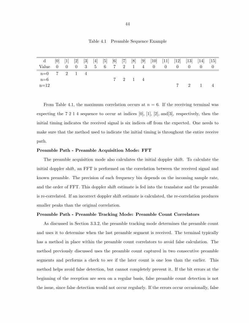
Table 4.1 Preamble Sequence Example
d [0] [1] [2] [3] [4] [5] [6] [7] [8] [9] [10] [11] [12] [13] [14] [15]Value 0 0 0 3 5 6 7 2 1 4 0 0 0 0 0 0
n=0 7 2 1 4n=6 7 2 1 4n=12 7 2 1 4
From Table 4.1, the maximum correlation occurs at n = 6. If the receiving terminal was
expecting the 7 2 1 4 sequence to occur at indices [0], [1], [2], and[3], respectively, then the
initial timing indicates the received signal is six indices off from the expected. One needs to
make sure that the method used to indicate the initial timing is throughout the entire receive
path.
Preamble Path - Preamble Acquisition Mode: FFT
The preamble acquisition mode also calculates the initial doppler shift. To calculate the
initial doppler shift, an FFT is performed on the correlation between the received signal and
known preamble. The precision of each frequency bin depends on the incoming sample rate,
and the order of FFT. This doppler shift estimate is fed into the translator and the preamble
is re-correlated. If an incorrect doppler shift estimate is calculated, the re-correlation produces
smaller peaks than the original correlation.
Preamble Path - Preamble Tracking Mode: Preamble Count Correlators
As discussed in Section 3.3.2, the preamble tracking mode determines the preamble count
and uses it to determine when the last preamble segment is received. The terminal typically
has a method in place within the preamble count correlators to avoid false calculation. The
method previously discussed uses the preamble count captured in two consecutive preamble
segments and performs a check to see if the later count is one less than the earlier. This
method helps avoid false detection, but cannot completely prevent it. If the bit errors at the
beginning of the reception are seen on a regular basis, false preamble count detection is not
the issue, since false detection would not occur regularly. If the errors occur occasionally, false
45
preamble count detection could be the issue and the incoming data should be captured. The
preamble count for each segment can be calculated if the interleaver length of the transmitting
terminal is known. A short interleaver produces 3 preamble segments and a long interleaver
produces 24 segments. By stepping through the code a comparison can be made between the
preamble count determined from the received signal and the known preamble count. Although
the probability is low, the received signal could have bit errors occur such that the preamble
count from two consecutive segments have a difference of one, but are still incorrect.
Preamble Path - End of Preamble Mode: Initialization for Data Mode
Section 3.3.3 describes the end of preamble mode. A major function of the end of preamble
mode is calculating a channel estimate and adjusting the timing position of the received signal.
During the end of preamble mode, an initial channel estimate is performed, to be used on the
first data frame. The channel estimate is calculated using the LMS algorithm discussed in
Section 3.4.2.1. The first step to ensure that the channel estimate is being calculated correctly
is to check the software logic against the LMS algorithm. Using Equation 4.1 and Section
3.4.2.1 as a reference, w[n] =∑L
k=0 I[k]h[n− k] and,
w[I[3]] = h[0]I[3] + h[1]I[2] + h[2]I[1] + h[3]I[0]
Following the LMS algorithm outlined, Equation 4.2 can be used to calculate e[n], where d[I[3]]
is located at index d[9].
e[I[3]] = d[I[3]]− w[I[3]]
= d[9]− w[I[3]]
It would be very easy to use the wrong indices when calculating the channel estimate. For
instance, rather than using the received symbol thought to be I[3], perhaps d[I[2]] is used
instead. The software implementing this algorithm needs to be checked very thoroughly. The
initial channel estimate is only used for the first frame of data, so bit errors occurring at the
beginning may be caused by an error in the LMS logic.
46
4.1.2 Errors at the End of the Reception
If bit errors occur at the end of the reception, the area of code to begin debugging is the
data path. As discussed in Section 3.4, the receive path contains a probe correlator, channel
estimator, matched filter, an equalizer and demodulator, a descrambler, deinterleaver, decoder
and an EOM detector. The main focus for errors occurring at the end of a reception is the
EOM detector. As discussed in Section 3.4.4, only the data bits prior to the EOM are sent to
the external interface.
Data Path - EOM Detector
One possible cause of bit errors may be related to bit boundary differences between the
transmitting and receiving terminals. For example, if the implementation of the transmitting
terminal is limited to 16-bit boundaries, rather than 8-bit boundaries, the valid data bits must
be zero-padded before the EOM is attached. If this is occurring the receiving terminal will see
less than 16 bits of padding prior to the EOM. Since the logic assumes all bits prior to the
EOM are valid, the extra zeros are sent to the external interface and logged as errors. The
only method to check if this is occuring is to check the decoder output. By sending all ones,
the data directly before the EOM should be ones, rather than zero-padding. If the data is
zero-padded, there is nothing the engineer can do except make a design change.
Another potential issue which causes bit errors at the end of the reception is the EOM
detection logic. The terminal may rely on the probe correlators to detect a signal loss and
mark the end of the reception, if the logic for EOM detection is incorrect. Bit errors could
occur if the EOM or data past the EOM is sent to the external interface. By checking the
output of the decoder, it can be determined whether or not the EOM is present. If the EOM is
never seen within the decoded bits, there may be a mismatch between the number of interleaver
flush bits sent by the transmitting terminal and the number of flush needed by the receiving
terminal.
47
4.1.3 Errors Throughout the Reception
If bit errors occur throughout the reception, both the preamble and data paths have po-
tential areas of interest. They include the initial doppler shift estimate within the preamble
acquisition mode, autobaud detection within the preamble tracking mode, the timing adjust-
ment performed during the end of preamble mode, and the deinterleaver with the data path.
Preamble Path - Preamble Acquisition Mode: FFT
According to the MIL-STD-188-110A [3], the single tone modem is only required to com-
pensate for a doppler shift of 75 Hz. Within the preamble acquisition mode, an initial doppler
shift estimate is performed by placing the correlation of the received signal and the known
preamble through an FFT. If the doppler shift is determined to be larger than 75 Hz, the
terminal will only correct for 75 leading to bit errors and loss of synchronization. By check-
ing the output of the FFT, it can be determined if the doppler shift is greater than 75 Hz.
If it is, corrections need to be made within the test equipment to stay within the military
specifications.
Preamble Path - Preamble Tracking Mode: Autobaud Information Correlators
During preamble tracking mode, the terminal correlates on all possible interleaver length
and data rate options to see which produces the greatest correlation peak. If the logic to
determine the autobaud information is wrong, the incorrect data rate or interleaver length
would cause bit errors throughout the reception. Compare the detected autobaud information
with the known transmitting terminal’s data rate and interleaver length to determine if they
were correctly received.
Preamble Path - End of Preamble Mode: Timing Adjustment
The other task performed by the end of preamble mode is a timing adjustment. From
Table 4.1, it was shown that the received signal was offset by six. To make data mode easier,
the received signal is internally shifted such that the boundary between the end of preamble
and data has an offset of zero. When performing this function, it is easy to make a mistake
associated with array indices. It is also easy to request an incorrect amount of samples from
the receiver during the first frame of data, since a portion of the first data frame was received
48
during the final preamble segment. Stepping through the software to check all logic is correct
is a quick and easy method to ensure a correct timing adjustment.
Data Path - Deinterleaver
If the bit errors are caused by the deinterleaver on the data path, it would be easy to
identify. The bit errors seen during the reception typically occur in a periodic manner and
the period may resemble the length of the selected deinterleaver. If the period does resemble
the deinterleaver length, one area of interest may be the logic within the deinterleaver which
switches between loading and unloading.
When bit errors occur during the beginning or the end of a reception, there are fewer
possible software issues, than when they occur in the middle of the reception. Typically, more
information needs to be obtained to further determine the area of software to debug. The bit
errors may be related to an AGC frequency dispersion issue. Perhaps the probe correlators
are not choosing the correct peak for time dispersion. There are many more blocks within the
data path that may be contributing to the bit errors received in the middle of the reception,
but more debug information is needed. Another method of capturing debug information is
to isolate the individual channel effects. By isolating each channel effect, software defects
associated with each issue are easier to isolate and debug.
4.2 Software Isolation using Channel Effects
In addition to using bit error timing to isolate the software issue, applying channel effects
individually is another method that should be used. Bit errors which occur because of terminal
clock differences indicate a different software issue than bit errors caused by frequency disper-
sion. By isolating individual channel effects, software defects relating to each can be debugged
before combining them together for performance testing.
It is generally easier to isolate the individual channel effects if the transmit and receive
software can be placed in an 8k sps loopback mode. By placing the modem in 8k sps loop-
back, the Single Tone modem software is completely isolated, yet the entire modem is tested.
To accomplish this, a loop is placed at the output of the transmit rate change filter to the
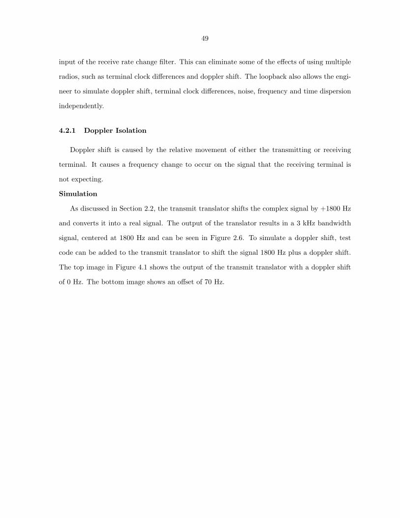
49
input of the receive rate change filter. This can eliminate some of the effects of using multiple
radios, such as terminal clock differences and doppler shift. The loopback also allows the engi-
neer to simulate doppler shift, terminal clock differences, noise, frequency and time dispersion
independently.
4.2.1 Doppler Isolation
Doppler shift is caused by the relative movement of either the transmitting or receiving
terminal. It causes a frequency change to occur on the signal that the receiving terminal is
not expecting.
Simulation
As discussed in Section 2.2, the transmit translator shifts the complex signal by +1800 Hz
and converts it into a real signal. The output of the translator results in a 3 kHz bandwidth
signal, centered at 1800 Hz and can be seen in Figure 2.6. To simulate a doppler shift, test
code can be added to the transmit translator to shift the signal 1800 Hz plus a doppler shift.
The top image in Figure 4.1 shows the output of the transmit translator with a doppler shift
of 0 Hz. The bottom image shows an offset of 70 Hz.
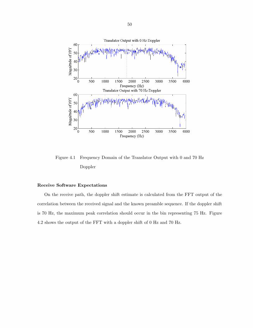
50
Figure 4.1 Frequency Domain of the Translator Output with 0 and 70 Hz
Doppler
Receive Software Expectations
On the receive path, the doppler shift estimate is calculated from the FFT output of the
correlation between the received signal and the known preamble sequence. If the doppler shift
is 70 Hz, the maximum peak correlation should occur in the bin representing 75 Hz. Figure
4.2 shows the output of the FFT with a doppler shift of 0 Hz and 70 Hz.
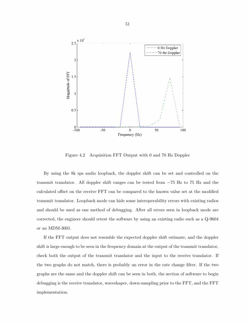
51
Figure 4.2 Acquisition FFT Output with 0 and 70 Hz Doppler
By using the 8k sps audio loopback, the doppler shift can be set and controlled on the
transmit translator. All doppler shift ranges can be tested from −75 Hz to 75 Hz and the
calculated offset on the receive FFT can be compared to the known value set at the modified
transmit translator. Loopback mode can hide some interoperability errors with existing radios
and should be used as one method of debugging. After all errors seen in loopback mode are
corrected, the engineer should retest the software by using an existing radio such as a Q-9604
or an MDM-3001.
If the FFT output does not resemble the expected doppler shift estimate, and the doppler
shift is large enough to be seen in the frequency domain at the output of the transmit translator,
check both the output of the transmit translator and the input to the receive translator. If
the two graphs do not match, there is probably an error in the rate change filter. If the two
graphs are the same and the doppler shift can be seen in both, the section of software to begin
debugging is the receive translator, waveshaper, down-sampling prior to the FFT, and the FFT
implementation.
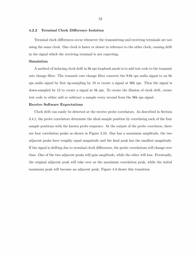
52
4.2.2 Terminal Clock Difference Isolation
Terminal clock differences occur whenever the transmitting and receiving terminals are not
using the same clock. One clock is faster or slower in reference to the other clock, causing drift
in the signal which the receiving terminal is not expecting.
Simulation
A method of inducing clock drift in 8k sps loopback mode is to add test code to the transmit
rate change filter. The transmit rate change filter converts the 9.6k sps audio signal to an 8k
sps audio signal by first up-sampling by 10 to create a signal at 96k sps. Then the signal is
down-sampled by 12 to create a signal at 8k sps. To create the illusion of clock drift, create
test code to either add or subtract a sample every second from the 96k sps signal.
Receive Software Expectations
Clock drift can easily be detected at the receive probe correlators. As described in Section
3.4.1, the probe correlators determine the ideal sample position by correlating each of the four
sample positions with the known probe sequence. At the output of the probe correlator, there
are four correlation peaks as shown in Figure 3.10. One has a maximum amplitude, the two
adjacent peaks have roughly equal magnitude and the final peak has the smallest magnitude.
If the signal is drifting due to terminal clock differences, the probe correlations will change over
time. One of the two adjacent peaks will gain amplitude, while the other will lose. Eventually,
the original adjacent peak will take over as the maximum correlation peak, while the initial
maximum peak will become an adjacent peak. Figure 4.3 shows this transition.
53
Figure 4.3 Original Probe Correlation and after Drift
As shown in Figure 4.3, the original probe correlation can be seen at the top image. The
maximum correlation peak occurs at the third sample position, while the second and fourth
peaks contain roughly equal power. As clock drift occurs, the second peak grows in power,
while the other adjacent peak weakens in power. The bottom image in Figure 4.3 shows the
second peaks growing enough in power to pass the third peak to become the new ideal sample
position.
One common method to solve clock drift is to force the probe correlations to stay stationary.
By monitoring the probe correlation peaks, samples can be added or subtracted in the receive
rate change filter. Correlation peak fluctuate naturally. Be sure a method is in place to ensure
any peak changes are not just natural fluctuations. For instance, when one of the two adjacent
peaks is a certain percentage higher than the other for a pre-determined time, the software
knows it is not natural fluctuation and signals the rate change filter that drift is occurring.
If the leading adjacent peak is greater than the lagging, then the receiving terminal’s clock is
running slower than the transmitting terminal’s clock. To compensate for this difference the
54
receive rate change filter drops samples to advance ahead and speed up the receive clock. If the
lagging adjacent peak is growing larger than the leading, then the receiving terminal’s clock
is running faster than the transmitting terminal’s clock. The receive rate change filter adds
samples to slow the receive clock as a method to compensate.
If the receiving terminal detects a signal loss, or the engineer observes the correlation peaks
changing in the debugger, this indicates that the logic to correct for terminal clock differences
is not working. First, check that the receive rate change filter is being instructed the same
command as the transmit rate change filter. If the test code is simulating clock drift by
slowing down the transmit clock, then the logic which keeps track of the adjacent correlator
peaks should instruct the receive rate change filter to also slow down. If the opposite command
is being given to the receive rate change filter, the engineer should begin debugging the logic
maintaining the adjacent correlator peaks.
The frequency of altering the transmit and receive clocks within the rate change filters
should also be checked. If the test code within the transmit rate change filter is adding or
subtracting one sample per second, then the receive rate change filter should also be adding or
subtracting at roughly the same rate. If the frequencies are not similar, the logic within the
probe correlators which determines how frequently the receive rate change filter is called needs
to be modified.
4.2.3 Noise Isolation
Noise occurs over any channel and can be thought of as a source of an additive random
signal. In the case of Single Tone, it is assumed to be AWGN.
Simulation
Two methods of simulating noise, frequency dispersion and time dispersion are: using a
software channel simulator in 8k sps loopback mode, and using an existing modem as a channel
simulator in audio mode. The first method inserts a software channel simulator within the 8k
sps audio loopback mode. The second method takes the modem software out of 8k sps loopback
mode, and uses two external, existing modems. Two examples of existing modems that could
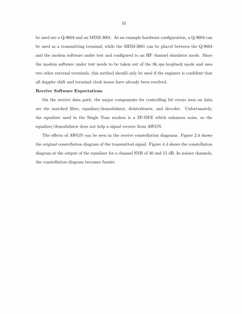
55
be used are a Q-9604 and an MDM-3001. As an example hardware configuration, a Q-9604 can
be used as a transmitting terminal, while the MDM-3001 can be placed between the Q-9604
and the modem software under test and configured to an HF channel simulator mode. Since
the modem software under test needs to be taken out of the 8k sps loopback mode and uses
two other external terminals, this method should only be used if the engineer is confident that
all doppler shift and terminal clock issues have already been resolved.
Receive Software Expectations
On the receive data path, the major components for controlling bit errors seen on data
are the matched filter, equalizer/demodulator, deinterleaver, and decoder. Unfortunately,
the equalizer used in the Single Tone modem is a ZF-DFE which enhances noise, so the
equalizer/demodulator does not help a signal recover from AWGN.
The effects of AWGN can be seen in the receive constellation diagrams. Figure 2.4 shows
the original constellation diagram of the transmitted signal. Figure 4.4 shows the constellation
diagram at the output of the equalizer for a channel SNR of 40 and 15 dB. In noisier channels,
the constellation diagram becomes fuzzier.
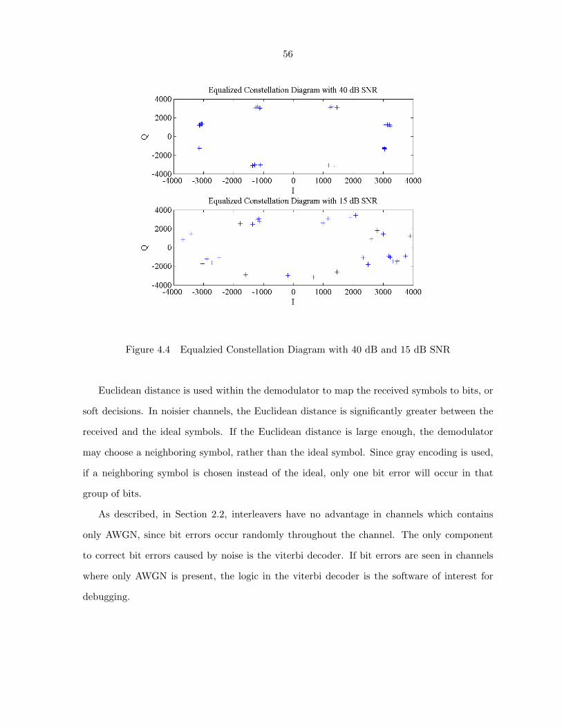
56
Figure 4.4 Equalzied Constellation Diagram with 40 dB and 15 dB SNR
Euclidean distance is used within the demodulator to map the received symbols to bits, or
soft decisions. In noisier channels, the Euclidean distance is significantly greater between the
received and the ideal symbols. If the Euclidean distance is large enough, the demodulator
may choose a neighboring symbol, rather than the ideal symbol. Since gray encoding is used,
if a neighboring symbol is chosen instead of the ideal, only one bit error will occur in that
group of bits.
As described, in Section 2.2, interleavers have no advantage in channels which contains
only AWGN, since bit errors occur randomly throughout the channel. The only component
to correct bit errors caused by noise is the viterbi decoder. If bit errors are seen in channels
where only AWGN is present, the logic in the viterbi decoder is the software of interest for
debugging.
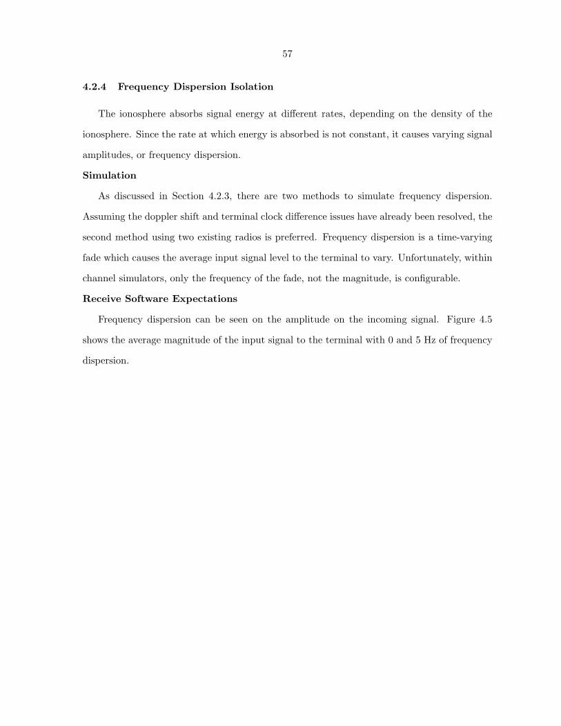
57
4.2.4 Frequency Dispersion Isolation
The ionosphere absorbs signal energy at different rates, depending on the density of the
ionosphere. Since the rate at which energy is absorbed is not constant, it causes varying signal
amplitudes, or frequency dispersion.
Simulation
As discussed in Section 4.2.3, there are two methods to simulate frequency dispersion.
Assuming the doppler shift and terminal clock difference issues have already been resolved, the
second method using two existing radios is preferred. Frequency dispersion is a time-varying
fade which causes the average input signal level to the terminal to vary. Unfortunately, within
channel simulators, only the frequency of the fade, not the magnitude, is configurable.
Receive Software Expectations
Frequency dispersion can be seen on the amplitude on the incoming signal. Figure 4.5
shows the average magnitude of the input signal to the terminal with 0 and 5 Hz of frequency
dispersion.
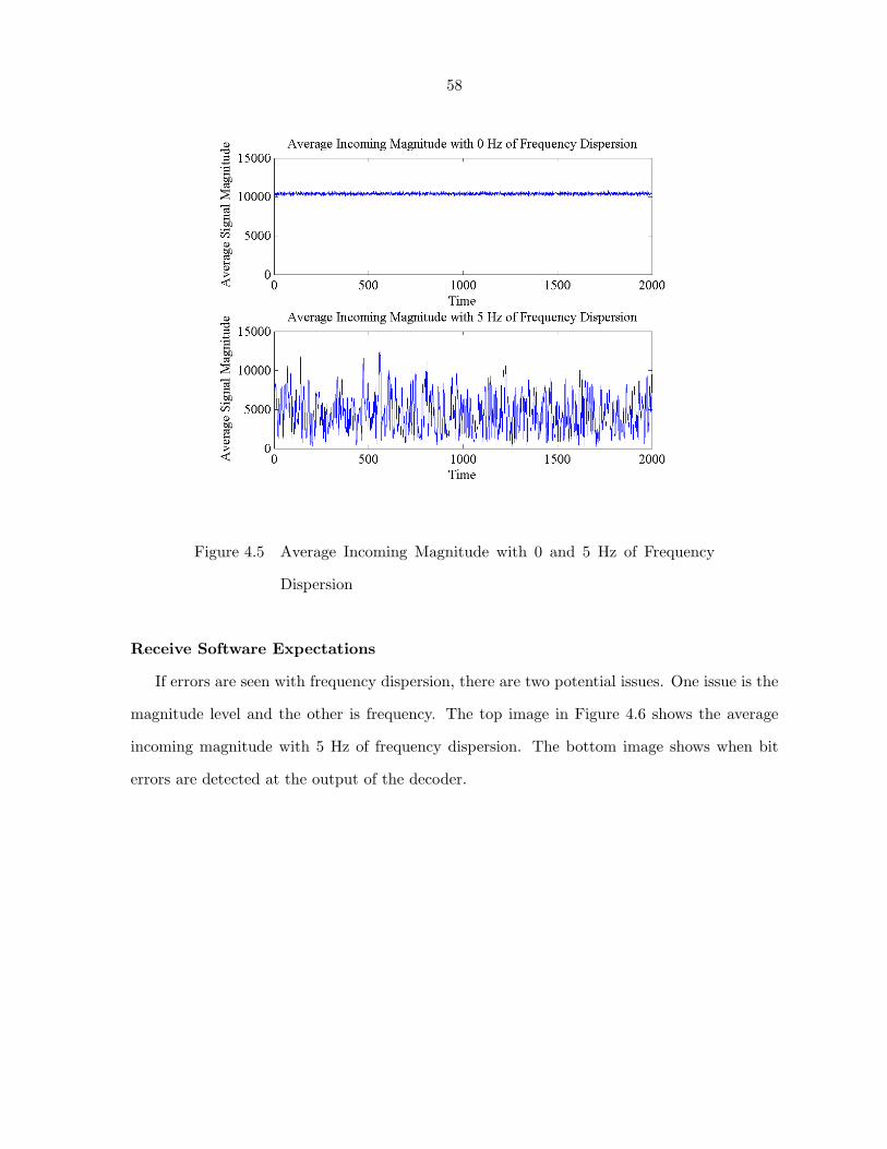
58
Figure 4.5 Average Incoming Magnitude with 0 and 5 Hz of Frequency
Dispersion
Receive Software Expectations
If errors are seen with frequency dispersion, there are two potential issues. One issue is the
magnitude level and the other is frequency. The top image in Figure 4.6 shows the average
incoming magnitude with 5 Hz of frequency dispersion. The bottom image shows when bit
errors are detected at the output of the decoder.
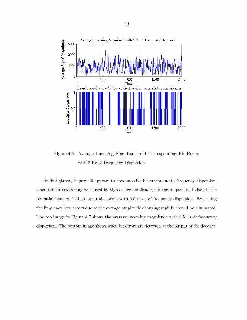
59
Figure 4.6 Average Incoming Magnitude and Corresponding Bit Errors
with 5 Hz of Frequency Dispersion
At first glance, Figure 4.6 appears to have massive bit errors due to frequency dispersion,
when the bit errors may be caused by high or low amplitude, not the frequency. To isolate the
potential issue with the magnitude, begin with 0.5 msec of frequency dispersion. By setting
the frequency low, errors due to the average amplitude changing rapidly should be eliminated.
The top image in Figure 4.7 shows the average incoming magnitude with 0.5 Hz of frequency
dispersion. The bottom image shows when bit errors are detected at the output of the decoder.
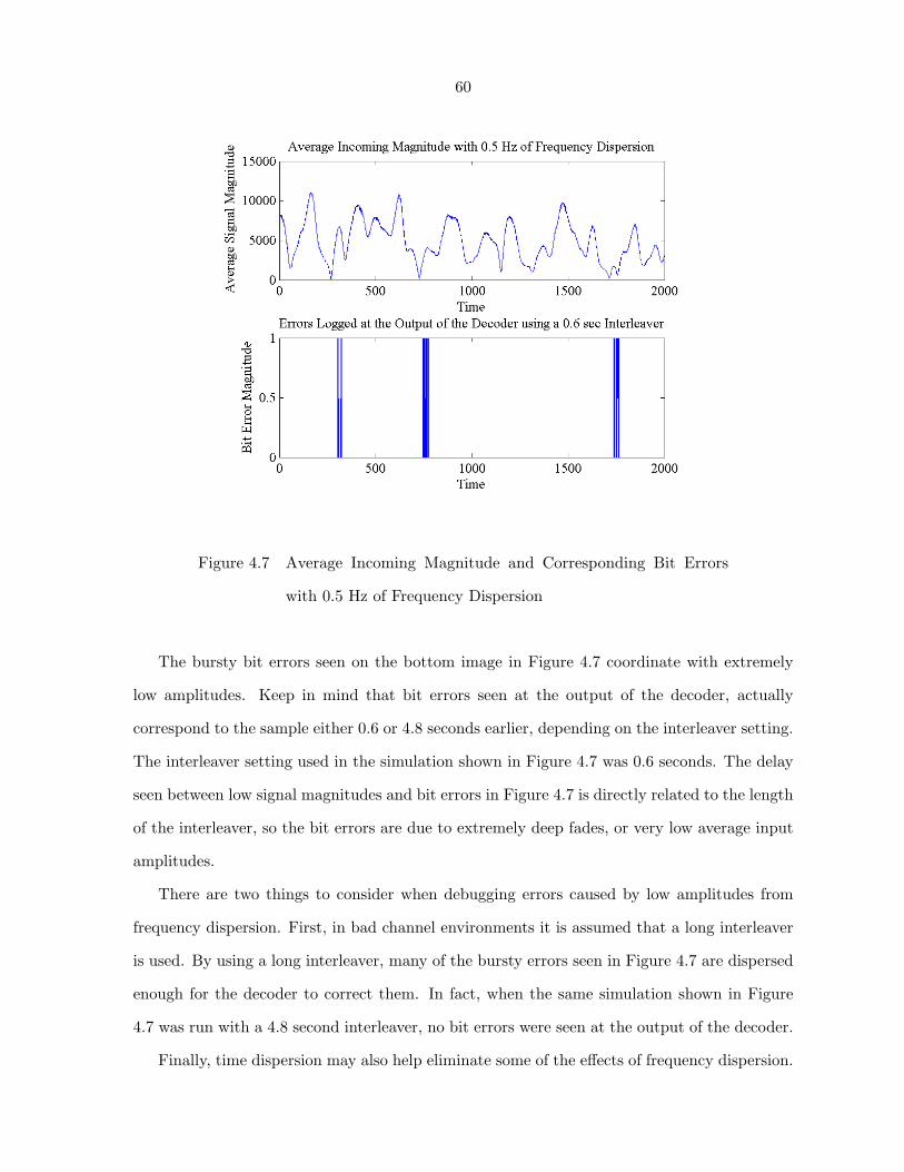
60
Figure 4.7 Average Incoming Magnitude and Corresponding Bit Errors
with 0.5 Hz of Frequency Dispersion
The bursty bit errors seen on the bottom image in Figure 4.7 coordinate with extremely
low amplitudes. Keep in mind that bit errors seen at the output of the decoder, actually
correspond to the sample either 0.6 or 4.8 seconds earlier, depending on the interleaver setting.
The interleaver setting used in the simulation shown in Figure 4.7 was 0.6 seconds. The delay
seen between low signal magnitudes and bit errors in Figure 4.7 is directly related to the length
of the interleaver, so the bit errors are due to extremely deep fades, or very low average input
amplitudes.
There are two things to consider when debugging errors caused by low amplitudes from
frequency dispersion. First, in bad channel environments it is assumed that a long interleaver
is used. By using a long interleaver, many of the bursty errors seen in Figure 4.7 are dispersed
enough for the decoder to correct them. In fact, when the same simulation shown in Figure
4.7 was run with a 4.8 second interleaver, no bit errors were seen at the output of the decoder.
Finally, time dispersion may also help eliminate some of the effects of frequency dispersion.
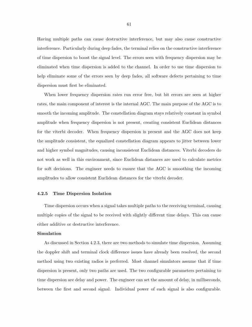
61
Having multiple paths can cause destructive interference, but may also cause constructive
interference. Particularly during deep fades, the terminal relies on the constructive interference
of time dispersion to boost the signal level. The errors seen with frequency dispersion may be
eliminated when time dispersion is added to the channel. In order to use time dispersion to
help eliminate some of the errors seen by deep fades, all software defects pertaining to time
dispersion must first be eliminated.
When lower frequency dispersion rates run error free, but bit errors are seen at higher
rates, the main component of interest is the internal AGC. The main purpose of the AGC is to
smooth the incoming amplitude. The constellation diagram stays relatively constant in symbol
amplitude when frequency dispersion is not present, creating consistent Euclidean distances
for the viterbi decoder. When frequency dispersion is present and the AGC does not keep
the amplitude consistent, the equalized constellation diagram appears to jitter between lower
and higher symbol magnitudes, causing inconsistent Euclidean distances. Viterbi decoders do
not work as well in this environment, since Euclidean distances are used to calculate metrics
for soft decisions. The engineer needs to ensure that the AGC is smoothing the incoming
amplitudes to allow consistent Euclidean distances for the viterbi decoder.
4.2.5 Time Dispersion Isolation
Time dispersion occurs when a signal takes multiple paths to the receiving terminal, causing
multiple copies of the signal to be received with slightly different time delays. This can cause
either additive or destructive interference.
Simulation
As discussed in Section 4.2.3, there are two methods to simulate time dispersion. Assuming
the doppler shift and terminal clock difference issues have already been resolved, the second
method using two existing radios is preferred. Most channel simulators assume that if time
dispersion is present, only two paths are used. The two configurable parameters pertaining to
time dispersion are delay and power. The engineer can set the amount of delay, in milliseconds,
between the first and second signal. Individual power of each signal is also configurable.
62
Additive and destructive interference escalates when the two signals have equal power, making
it the hardest power difference to recover from.
Receive Software Expectations
Time dispersion is visible at the receive probe correlators. The top image in Figure 4.8
shows an example of a normal probe correlation. The bottom image shows a correlation with
5 msec of time dispersion.
Figure 4.8 Probe Correlation with 0 msec and 5 msec of Time Dispersion
The first item to check is the delay seen within the probe correlators. Assume the incoming
symbol rate to the probe correlators is 2400 symbols per second. The expected delay within
the probe correlators is 2400 symbolssecond 0.005 seconds = 12 symbols. It can be seen in Figure
4.8 that the smaller peak is 12 symbols from the larger peak. If the time dispersion seen in
the probe correlations does not match the delay set at the channel simulator, re-check the
hardware setup and the channel simulator settings.
If errors are seen with time dispersion, there are two potential issues. One issue is the delay
between the two paths, and the other is the power difference. To isolate the potential issue
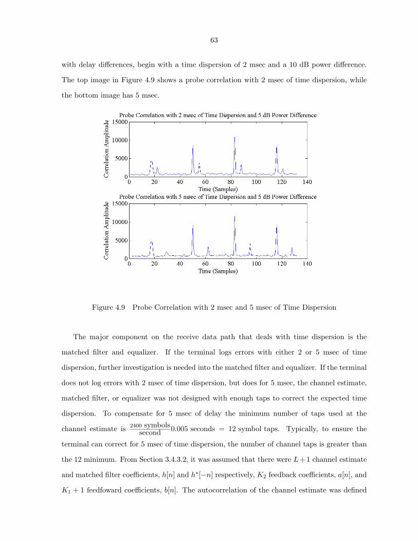
63
with delay differences, begin with a time dispersion of 2 msec and a 10 dB power difference.
The top image in Figure 4.9 shows a probe correlation with 2 msec of time dispersion, while
the bottom image has 5 msec.
Figure 4.9 Probe Correlation with 2 msec and 5 msec of Time Dispersion
The major component on the receive data path that deals with time dispersion is the
matched filter and equalizer. If the terminal logs errors with either 2 or 5 msec of time
dispersion, further investigation is needed into the matched filter and equalizer. If the terminal
does not log errors with 2 msec of time dispersion, but does for 5 msec, the channel estimate,
matched filter, or equalizer was not designed with enough taps to correct the expected time
dispersion. To compensate for 5 msec of delay the minimum number of taps used at the
channel estimate is 2400 symbolssecond 0.005 seconds = 12 symbol taps. Typically, to ensure the
terminal can correct for 5 msec of time dispersion, the number of channel taps is greater than
the 12 minimum. From Section 3.4.3.2, it was assumed that there were L+ 1 channel estimate
and matched filter coefficients, h[n] and h∗[−n] respectively, K2 feedback coefficients, a[n], and
K1 + 1 feedfoward coefficients, b[n]. The autocorrelation of the channel estimate was defined
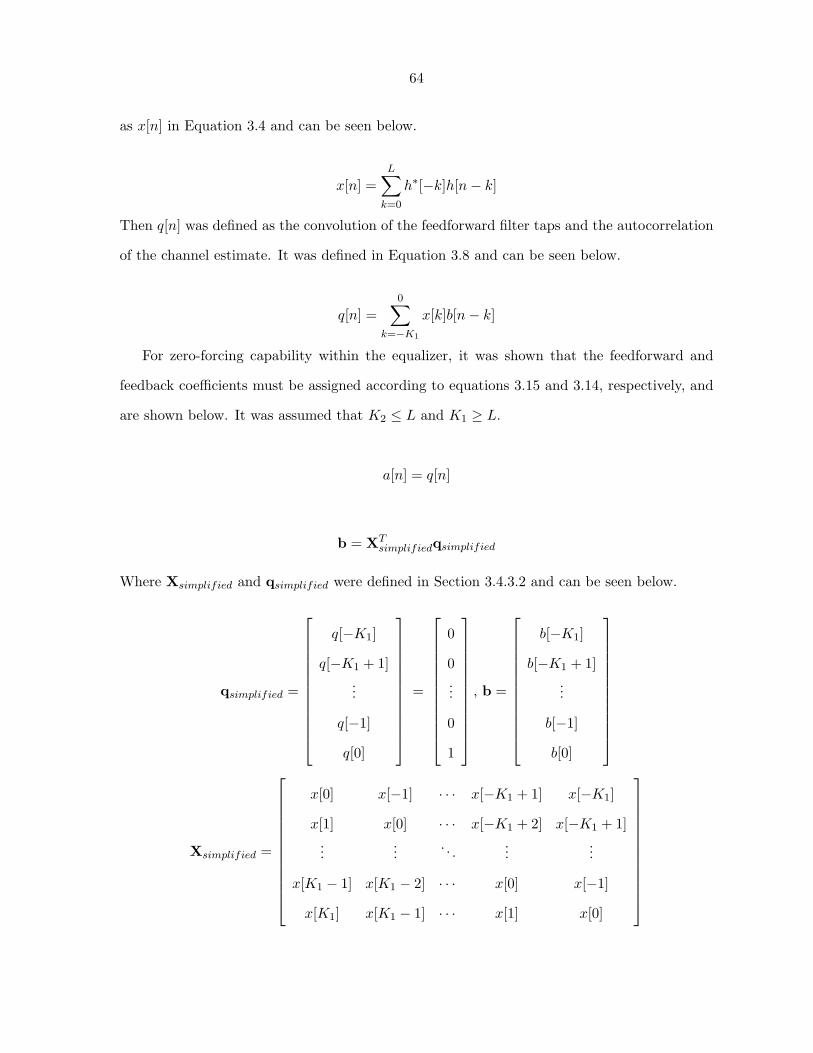
64
as x[n] in Equation 3.4 and can be seen below.
x[n] =L∑k=0
h∗[−k]h[n− k]
Then q[n] was defined as the convolution of the feedforward filter taps and the autocorrelation
of the channel estimate. It was defined in Equation 3.8 and can be seen below.
q[n] =0∑
k=−K1
x[k]b[n− k]
For zero-forcing capability within the equalizer, it was shown that the feedforward and
feedback coefficients must be assigned according to equations 3.15 and 3.14, respectively, and
are shown below. It was assumed that K2 ≤ L and K1 ≥ L.
a[n] = q[n]
b = XTsimplifiedqsimplified
Where Xsimplified and qsimplified were defined in Section 3.4.3.2 and can be seen below.
qsimplified =
q[−K1]
q[−K1 + 1]...
q[−1]
q[0]
=
0
0...
0
1
, b =
b[−K1]
b[−K1 + 1]...
b[−1]
b[0]
Xsimplified =
x[0] x[−1] · · · x[−K1 + 1] x[−K1]
x[1] x[0] · · · x[−K1 + 2] x[−K1 + 1]...
.... . .
......
x[K1 − 1] x[K1 − 2] · · · x[0] x[−1]
x[K1] x[K1 − 1] · · · x[1] x[0]
65
To initialize these filter coefficients, it is assumed a correct channel estimate was taken.
Check the channel estimate logic to be sure it matches the LMS algorithm described in Section
3.4.2.1. Mistakes can easily be made with array indices when performing signal mathematics.
Be sure the correct array indices are used for I[n] and h[n] when calculating w[n] and that
the correct corresponding d[n] is used to calculate e[n]. Assume n = 3rd symbol in the probe.
Then,
w[3rd symbol in the probe] =L∑k=0
h[k]I[3rd symbol in the probe− k]
where I[3rd symbol in the probe is the 3rd symbol in the known probe, and
e[3rd symbol in the probe] = d[3rd symbol in the probe]− w[3rd symbol in the probe]
where d[3rd symbol in the probe] is the received symbol believed to be the 3rd symbol in the
probe based upon the preamble and probe correlations.
To isolate the other potential issue with equal power on both paths, use a time dispersion
of 2 msec, but similar power. The top image in Figure 4.10 shows the probe correlation with
a power difference of 5dB, while the bottom image has 0 dB power difference. Both images
were created with a time dispersion of 5msec.
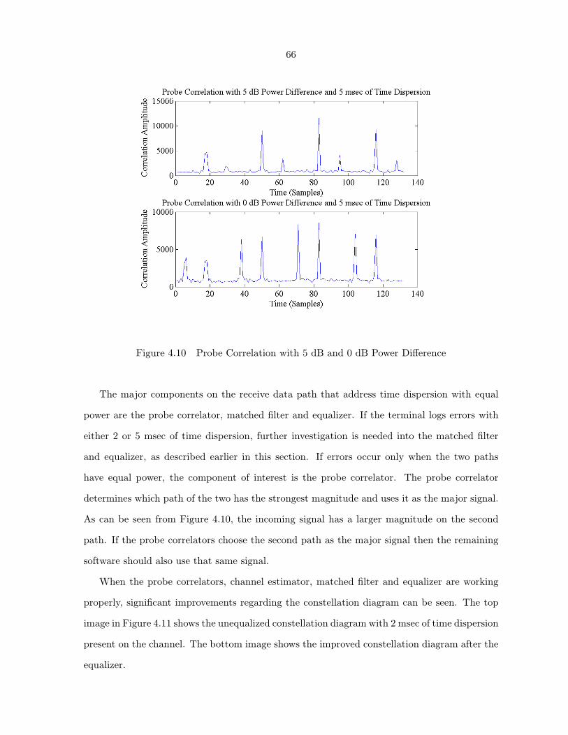
66
Figure 4.10 Probe Correlation with 5 dB and 0 dB Power Difference
The major components on the receive data path that address time dispersion with equal
power are the probe correlator, matched filter and equalizer. If the terminal logs errors with
either 2 or 5 msec of time dispersion, further investigation is needed into the matched filter
and equalizer, as described earlier in this section. If errors occur only when the two paths
have equal power, the component of interest is the probe correlator. The probe correlator
determines which path of the two has the strongest magnitude and uses it as the major signal.
As can be seen from Figure 4.10, the incoming signal has a larger magnitude on the second
path. If the probe correlators choose the second path as the major signal then the remaining
software should also use that same signal.
When the probe correlators, channel estimator, matched filter and equalizer are working
properly, significant improvements regarding the constellation diagram can be seen. The top
image in Figure 4.11 shows the unequalized constellation diagram with 2 msec of time dispersion
present on the channel. The bottom image shows the improved constellation diagram after the
equalizer.
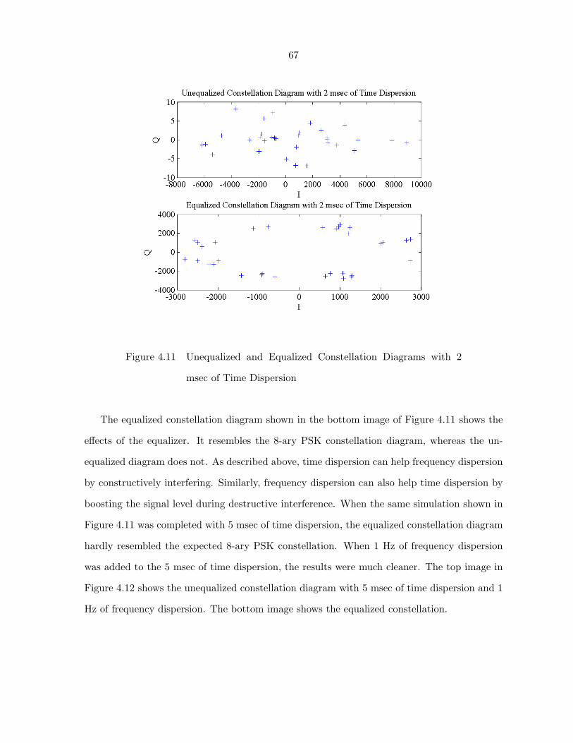
67
Figure 4.11 Unequalized and Equalized Constellation Diagrams with 2
msec of Time Dispersion
The equalized constellation diagram shown in the bottom image of Figure 4.11 shows the
effects of the equalizer. It resembles the 8-ary PSK constellation diagram, whereas the un-
equalized diagram does not. As described above, time dispersion can help frequency dispersion
by constructively interfering. Similarly, frequency dispersion can also help time dispersion by
boosting the signal level during destructive interference. When the same simulation shown in
Figure 4.11 was completed with 5 msec of time dispersion, the equalized constellation diagram
hardly resembled the expected 8-ary PSK constellation. When 1 Hz of frequency dispersion
was added to the 5 msec of time dispersion, the results were much cleaner. The top image in
Figure 4.12 shows the unequalized constellation diagram with 5 msec of time dispersion and 1
Hz of frequency dispersion. The bottom image shows the equalized constellation.
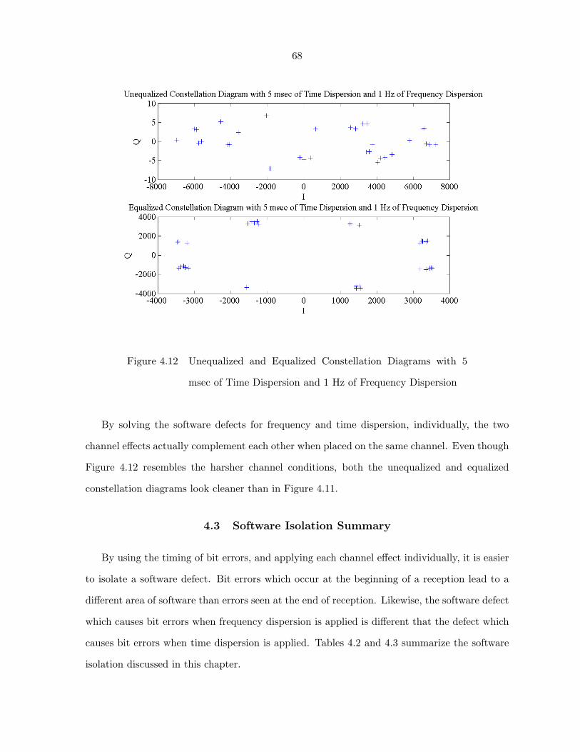
68
Figure 4.12 Unequalized and Equalized Constellation Diagrams with 5
msec of Time Dispersion and 1 Hz of Frequency Dispersion
By solving the software defects for frequency and time dispersion, individually, the two
channel effects actually complement each other when placed on the same channel. Even though
Figure 4.12 resembles the harsher channel conditions, both the unequalized and equalized
constellation diagrams look cleaner than in Figure 4.11.
4.3 Software Isolation Summary
By using the timing of bit errors, and applying each channel effect individually, it is easier
to isolate a software defect. Bit errors which occur at the beginning of a reception lead to a
different area of software than errors seen at the end of reception. Likewise, the software defect
which causes bit errors when frequency dispersion is applied is different that the defect which
causes bit errors when time dispersion is applied. Tables 4.2 and 4.3 summarize the software
isolation discussed in this chapter.
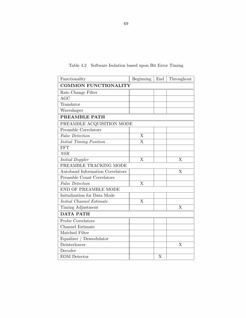
69
Table 4.2 Software Isolation based upon Bit Error Timing
Functionality Beginning End Throughout
COMMON FUNCTIONALITY
Rate Change FilterAGCTranslatorWaveshaper
PREAMBLE PATH
PREAMBLE ACQUISITION MODEPreamble CorrelatorsFalse Detection XInitial Timing Position XFFTNSRInitial Doppler X XPREAMBLE TRACKING MODEAutobaud Information Correlators XPreamble Count CorrelatorsFalse Detection XEND OF PREAMBLE MODEInitialization for Data ModeInitial Channel Estimate XTiming Adjustment X
DATA PATH
Probe CorrelatorsChannel EstimateMatched FilterEqualizer / DemodulatorDeinterleaver XDecoderEOM Detector X
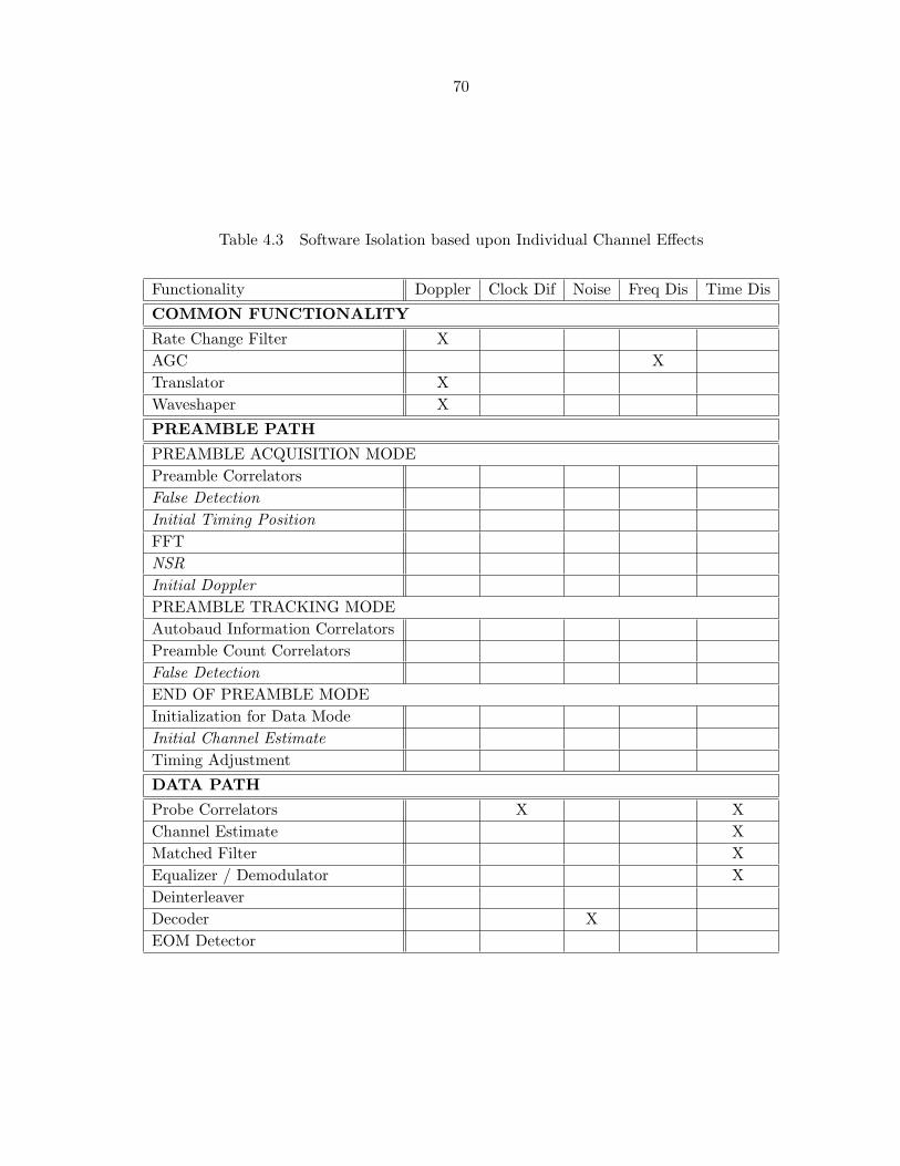
70
Table 4.3 Software Isolation based upon Individual Channel Effects
Functionality Doppler Clock Dif Noise Freq Dis Time Dis
COMMON FUNCTIONALITY
Rate Change Filter XAGC XTranslator XWaveshaper X
PREAMBLE PATH
PREAMBLE ACQUISITION MODEPreamble CorrelatorsFalse DetectionInitial Timing PositionFFTNSRInitial DopplerPREAMBLE TRACKING MODEAutobaud Information CorrelatorsPreamble Count CorrelatorsFalse DetectionEND OF PREAMBLE MODEInitialization for Data ModeInitial Channel EstimateTiming Adjustment
DATA PATH
Probe Correlators X XChannel Estimate XMatched Filter XEqualizer / Demodulator XDeinterleaverDecoder XEOM Detector
71
CHAPTER 5. SUMMARY AND FUTURE WORK
This thesis provides a new HF engineer some debugging techniques for the Single Tone
modem. In the future, this work can be expanded and explained in further detail. New
tests and isolation techniques can be added to further expand the debugging tree. Automated
testing could also be integrated with the information contained within this thesis. When the
testing software logs an error, it could also log the bit error timing, and any channel effects
for easier debugging. Single Tone is one of many HF modems. It would be beneficial to
have similar documents for the other HF modems. While researching the architecture, it was
discovered that there are many areas where better techniques could be applied. By writing
this type of document, each section of software can be looked at in detail and determine if
better implementation techniques are available.
The MIL-STD-188-110A Single Tone high frequency modem is used by the United States
military as a beyond line-of-sight radio which uses the ionosphere for reflection, rather than
a satellite. The HF Single Tone modem needs to account for typical channel effects such as
doppler shift, terminal clock differences, and noise in addition to some channel effects caused
by the ionosphere such as frequency and time dispersion. The signal processing software can
be difficult to debug when failures occur during performance testing. This thesis provides a
method of debugging by concentrating on two major steps: understanding and isolation. The
engineer must understand the channel model and receive path in order to correlate a test failure
with a specific section of software. This thesis provides a description of both the channel model
and receive path. After the channel model and receive path are understood, isolation of a test
failure through timing patterns of bit errors and individual channel effects help the engineer
isolate the software defect. This thesis creates a matrix of test failures with software isolation

72
of which to use for debugging.
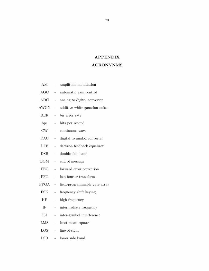
73
APPENDIX
ACRONYNMS
AM - amplitude modulation
AGC - automatic gain control
ADC - analog to digital converter
AWGN - additive white gaussian noise
BER - bir error rate
bps - bits per second
CW - continuous wave
DAC - digital to analog converter
DFE - decision feedback equalizer
DSB - double side band
EOM - end of message
FEC - forward error correction
FFT - fast fourier transform
FPGA - field-programmable gate array
FSK - frequency shift keying
HF - high frequency
IF - intermediate frequency
ISI - inter-symbol interference
LMS - least mean square
LOS - line-of-sight
LSB - lower side band
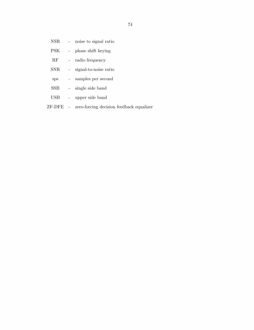
74
NSR - noise to signal ratio
PSK - phase shift keying
RF - radio frequency
SNR - signal-to-noise ratio
sps - samples per second
SSB - single side band
USB - upper side band
ZF-DFE - zero-forcing decision feedback equalizer
75
BIBLIOGRAPHY
[1] John W. Neito, On-Air results of Spatial Diversity for the MIL-STD-188-110B Appendix
C (STANAG 4539) 9600 bps waveform, IEEE 2001, pp. 432–436
[2] Collins Defense Communications, Publ. 523-0767157-002217, HF Communications Data
Book, June 1978
[3] MIL-STD-188-110A, Mil. Std. Interoperability and Performance Standards for Data
Modems, US Dept of Defense, September 1991
[4] MIL-STD-188-110B, Mil. Std. Interoperability and Performance Standards for Data
Modems, US Dept of Defense, March 1999
[5] J. Proakis, Digital Communication, McGraw Hill, ISBN 0-07-232111-3, 4th Edition
[6] W. N. Furman and J. W. Nieto Understanding HF Channel Simulator Requirements in
order to Reduce HF Modem Performance Measurement Variability
[7] Equations for the Raised Cosine and Square-Root Raised Cosine Shapes Brigham
Young University Department of Electrical and Computer Engineering 25 October 2008
http://www.ee.byu.edu/class/ee485public/ee485.fall.99/lectures/raised-cosine.pdf
76
ACKNOWLEDGEMENTS
I would like to take this opportunity to express my thanks to those who helped me con-
duct my research. Thank you to Dr. Zhengdao Wang for his guidance, patience and support
throughout this process. To my other committee members, Dr. Robert Weber and Dr. Alek-
sandar Dogandzic, thank you for agreeing to serve on my committee. Thanks to Pam Myers
for all of her help. Also, thanks to the entire DSP team at Rockwell Collins for their expertise.


![ECE-V-DIGITAL SIGNAL PROCESSING [10EC52] …vtusolution.in/.../digital-signal-processing-10ec52.pdfDigital vtusolution.in Signal Processing 10EC52 TEXT BOOK: 1. DIGITAL SIGNAL PROCESSING](https://img.pdfslide.net/doc/110x75/5afe42bb7f8b9a256b8ccd2e/ece-v-digital-signal-processing-10ec52-signal-processing-10ec52-text-book.jpg)