Embed Size (px)
Citation preview

Architectures and design patterns for functionaldesign of logic control and diagnostics in
industrial automation
Ph.D. Thesis
Matteo Sartini
Tutor: Prof. Claudio Bonivento
Coordinator: Prof. Claudio Melchiorri
University of Bologna
XXII Ciclo
A.A. 2006 – 2009

Architectures and design patterns for functionaldesign of logic control and diagnostics in
industrial automation.Ph.D. Thesis
Matteo Sartini
Tutor: Prof. Claudio Bonivento
Coordinator: Prof. Claudio Melchiorri
University of Bologna
XXII Ciclo
A.A. 2006 – 2009

Keywords:
Architectural Design Patterns, Fault Diagnosis, Discrete Event Systems, Automated Manufac-turing Systems, Model Driven Engineering.
Ing. Matteo SartiniCASY - DEIS - University of BolognaViale Pepoli 3/2, 40136 Bologna.Phone: +39 051 2093870, Fax: +39 051 2093871Email: [email protected]: http://www-lar.deis.unibo.it/people/msartini
This thesis has been written in LATEX.
Copyright c©2010 by Matteo Sartini. All rights reserved.
No part of this publication may be reproduced or transmitted in any form or by any means,electronic or mechanical, including photocopy, recording or any information storage and re-trieval system, without permission in writing from the author.
Acknowledgments:This work has been partially funded by the European Artemis Joint Undertaking funded projectCESAR: Cost-Efficient methods and processes for SAfety Relevant embedded systems, sponsored bythe European Commission in the IST programme 2008 of the 7th EC framework programme(ARTEMIS-2008-1).
This work has been partially funded by MIUR (Ministero dell’istruzione, dell’università e dellaricerca).

To Anna
SOONER OR LATER,THE WORST POSSIBLE COMBINATION OF CIRCUMSTANCES
WILL HAPPEN.
SODD’S LAW.
IN THEORY THERE IS NO DIFFERENCE BETWEEN THEORY AND PRACTICE.IN PRACTICE THERE IS.
YOGI BERRA.


Contents
Preface 15
1 Control design in industrial automated systems 231.1 Design specification in industrial automated system . . . . . . . . . . . . . . . . . 231.2 Classification of industrial automated systems . . . . . . . . . . . . . . . . . . . . 25
1.2.1 Assembly machines . . . . . . . . . . . . . . . . . . . . . . . . . . . . . . . 261.2.2 Inspection machines . . . . . . . . . . . . . . . . . . . . . . . . . . . . . . . 271.2.3 Test machines . . . . . . . . . . . . . . . . . . . . . . . . . . . . . . . . . . . 271.2.4 Packaging machines . . . . . . . . . . . . . . . . . . . . . . . . . . . . . . . 281.2.5 Computer numerical control machines . . . . . . . . . . . . . . . . . . . . 281.2.6 Production Processes . . . . . . . . . . . . . . . . . . . . . . . . . . . . . . . 29
1.3 Conclusions . . . . . . . . . . . . . . . . . . . . . . . . . . . . . . . . . . . . . . . . 31
2 State of the art of software engineering in industrial automated systems 332.1 Software architecture in industrial automation . . . . . . . . . . . . . . . . . . . . 332.2 Design patterns in industrial automation . . . . . . . . . . . . . . . . . . . . . . . 35
2.2.1 A design pattern for control process - S88 . . . . . . . . . . . . . . . . . . . 362.2.2 A design pattern for manufacturing systems - GEMMA . . . . . . . . . . . 39
2.3 Standard language in industrial automation . . . . . . . . . . . . . . . . . . . . . . 422.3.1 Standard language: IEC 61131-3 . . . . . . . . . . . . . . . . . . . . . . . . 432.3.2 Standard language: IEC 61499 . . . . . . . . . . . . . . . . . . . . . . . . . 47
2.4 Object Oriented . . . . . . . . . . . . . . . . . . . . . . . . . . . . . . . . . . . . . . 502.4.1 UML - Unified Modeling Language . . . . . . . . . . . . . . . . . . . . . . 51
2.5 Conclusions . . . . . . . . . . . . . . . . . . . . . . . . . . . . . . . . . . . . . . . . 53
3 Architecture in industrial automation: The Generalized Actuator approach 573.1 Introduction . . . . . . . . . . . . . . . . . . . . . . . . . . . . . . . . . . . . . . . . 573.2 Classic design procedure . . . . . . . . . . . . . . . . . . . . . . . . . . . . . . . . . 583.3 Generalized Actuator approach . . . . . . . . . . . . . . . . . . . . . . . . . . . . . 633.4 Generalized actuator definition and design procedure formalization . . . . . . . 65
3.4.1 Types of actions . . . . . . . . . . . . . . . . . . . . . . . . . . . . . . . . . . 683.5 GA in rapid prototyping . . . . . . . . . . . . . . . . . . . . . . . . . . . . . . . . . 693.6 Conclusions . . . . . . . . . . . . . . . . . . . . . . . . . . . . . . . . . . . . . . . . 74
5

6 Contents
4 The Generalized Device concept 774.1 Actuation mechanism . . . . . . . . . . . . . . . . . . . . . . . . . . . . . . . . . . 774.2 Devices classification . . . . . . . . . . . . . . . . . . . . . . . . . . . . . . . . . . . 804.3 A hierarchical multi-layer architecture . . . . . . . . . . . . . . . . . . . . . . . . . 824.4 The Generalized Devices . . . . . . . . . . . . . . . . . . . . . . . . . . . . . . . . . 854.5 Fault diagnosis functionalities . . . . . . . . . . . . . . . . . . . . . . . . . . . . . . 914.6 Conclusions . . . . . . . . . . . . . . . . . . . . . . . . . . . . . . . . . . . . . . . . 96
5 A discrete event approach to fault diagnosis in automated system 975.1 Formal verification in industrial automation . . . . . . . . . . . . . . . . . . . . . 975.2 A DES approach for formal verification . . . . . . . . . . . . . . . . . . . . . . . . 99
5.2.1 Architecture for supervisory control in industrial automation . . . . . . . 1005.2.2 Model building methodology . . . . . . . . . . . . . . . . . . . . . . . . . . 1025.2.3 Low level . . . . . . . . . . . . . . . . . . . . . . . . . . . . . . . . . . . . . 1035.2.4 Modeling fault at low level . . . . . . . . . . . . . . . . . . . . . . . . . . . 1065.2.5 Control and monitoring of low level devices . . . . . . . . . . . . . . . . . 110
5.3 Conclusions on DES approach for formal verification . . . . . . . . . . . . . . . . 1185.4 Active fault tolerant control online diagnostics . . . . . . . . . . . . . . . . . . . . 121
5.4.1 Fault tolerant control . . . . . . . . . . . . . . . . . . . . . . . . . . . . . . . 1215.4.2 Supervisory control of DES with faults . . . . . . . . . . . . . . . . . . . . 1225.4.3 Safe controllability of DES . . . . . . . . . . . . . . . . . . . . . . . . . . . . 1255.4.4 Active fault tolerance of DES . . . . . . . . . . . . . . . . . . . . . . . . . . 1275.4.5 An illustrative example . . . . . . . . . . . . . . . . . . . . . . . . . . . . . 1305.4.6 Conclusions on active fault tolerant control using online diagnostic . . . . 133
Conclusions and future works 135
A Introduction to discrete event systems theory 139A.1 Discrete event systems . . . . . . . . . . . . . . . . . . . . . . . . . . . . . . . . . . 139A.2 Operations on Languages . . . . . . . . . . . . . . . . . . . . . . . . . . . . . . . . 140A.3 Representation of languages: automata . . . . . . . . . . . . . . . . . . . . . . . . 141
A.3.1 Operations on automata . . . . . . . . . . . . . . . . . . . . . . . . . . . . . 142A.3.2 Observer automata . . . . . . . . . . . . . . . . . . . . . . . . . . . . . . . . 144
A.4 Regular languages . . . . . . . . . . . . . . . . . . . . . . . . . . . . . . . . . . . . 145A.5 Supervisory control . . . . . . . . . . . . . . . . . . . . . . . . . . . . . . . . . . . . 146A.6 Uncontrollability problem . . . . . . . . . . . . . . . . . . . . . . . . . . . . . . . . 148
A.6.1 Dealing with uncontrollable events . . . . . . . . . . . . . . . . . . . . . . 148A.6.2 Realization of supervisors . . . . . . . . . . . . . . . . . . . . . . . . . . . . 148
A.7 Unobservability problem . . . . . . . . . . . . . . . . . . . . . . . . . . . . . . . . . 149
B The demonstrator 151B.1 Testbed description . . . . . . . . . . . . . . . . . . . . . . . . . . . . . . . . . . . . 151
B.1.1 Distribution station . . . . . . . . . . . . . . . . . . . . . . . . . . . . . . . . 152B.1.2 Testing station . . . . . . . . . . . . . . . . . . . . . . . . . . . . . . . . . . . 154B.1.3 Processing Station . . . . . . . . . . . . . . . . . . . . . . . . . . . . . . . . 156B.1.4 Assembly station . . . . . . . . . . . . . . . . . . . . . . . . . . . . . . . . . 158
B.2 Part of code of FESTO . . . . . . . . . . . . . . . . . . . . . . . . . . . . . . . . . . 161

Contents 7
C Components models of DES approach 167C.1 Examples of model composition . . . . . . . . . . . . . . . . . . . . . . . . . . . . 167C.2 Control and monitoring of low level devices . . . . . . . . . . . . . . . . . . . . . 175
Bibliography 180
Index 187
Curriculum vitae 191

8 Contents
List of Figures
1.1 Control systems architecture evolution. . . . . . . . . . . . . . . . . . . . . . . . . 241.2 Control system architecture in automated systems. . . . . . . . . . . . . . . . . . 251.3 Example of industrial automated machine. . . . . . . . . . . . . . . . . . . . . . . 261.4 Example of a classic CNC machine. . . . . . . . . . . . . . . . . . . . . . . . . . . 291.5 Example of production process machine for a gasification process. . . . . . . . . 30
2.1 Example of S88 design pattern. . . . . . . . . . . . . . . . . . . . . . . . . . . . . . 382.2 Gemma architecture state. . . . . . . . . . . . . . . . . . . . . . . . . . . . . . . . . 412.3 The IEC 61131-3 software model. . . . . . . . . . . . . . . . . . . . . . . . . . . . . 442.4 A simple ladder diagram example. . . . . . . . . . . . . . . . . . . . . . . . . . . . 452.5 A simple FBD example. . . . . . . . . . . . . . . . . . . . . . . . . . . . . . . . . . 462.6 Example of 61131-3 function block connection. . . . . . . . . . . . . . . . . . . . . 472.7 Using 61131-3 function block with enable. . . . . . . . . . . . . . . . . . . . . . . 482.8 61499 Function block definition. . . . . . . . . . . . . . . . . . . . . . . . . . . . . 492.9 Example of UML diagram. . . . . . . . . . . . . . . . . . . . . . . . . . . . . . . . 522.10 Comparison between objects and function blocks. . . . . . . . . . . . . . . . . . . 54
3.1 Drilling module of Festo FMS. . . . . . . . . . . . . . . . . . . . . . . . . . . . . . 593.2 “Common” SFC solution for the case in example . . . . . . . . . . . . . . . . . . . 603.3 “Common” SFC solution for the case in example with new specification. . . . . . 613.4 “Common” SFC solution for the case in example with fault. . . . . . . . . . . . . 623.5 “Common” SFC solution for the case in example with new specification and fault. 633.6 Actions, sensors and actuators of the systems. . . . . . . . . . . . . . . . . . . . . 643.7 Interfaces of GAs. . . . . . . . . . . . . . . . . . . . . . . . . . . . . . . . . . . . . 673.8 Characteristics of Do/Done actions (a) and Start/Stop actions (b) . . . . . . . . . 683.9 Characteristic of GAs action. . . . . . . . . . . . . . . . . . . . . . . . . . . . . . . 693.10 Processing station. . . . . . . . . . . . . . . . . . . . . . . . . . . . . . . . . . . . . 703.11 Hierarchical GA DrillingUnitTotal. . . . . . . . . . . . . . . . . . . . . . . . . . . . 733.12 An example of policy manager with GA approach. . . . . . . . . . . . . . . . . . . 74
4.1 Device in industrial automation . . . . . . . . . . . . . . . . . . . . . . . . . . . . . 794.2 Single acting device using a double acting cylinder . . . . . . . . . . . . . . . . . . 804.3 Double acting device using a double acting cylinder . . . . . . . . . . . . . . . . . 814.4 Different type of devices: single acting devices (a) and double acting devices (b) . 824.5 The proposed hierarchical multi-layer architecture. . . . . . . . . . . . . . . . . . 83
9

10 LIST OF FIGURES
4.6 The miniaturized AMS used as test bed. . . . . . . . . . . . . . . . . . . . . . . . 844.7 The hierarchical multi layer architecture envisaged for the control of the AMS
used as test bed. . . . . . . . . . . . . . . . . . . . . . . . . . . . . . . . . . . . . . 864.8 The SADF GD and its interfaces. . . . . . . . . . . . . . . . . . . . . . . . . . . . . 864.9 FMS modeling the behavior of the SADF GD. . . . . . . . . . . . . . . . . . . . . 874.10 State diagram for the single acting GD with double feedback . . . . . . . . . . . . 884.11 State diagram for the single acting GD with double feedback . . . . . . . . . . . . 894.12 State diagram for the double acting GD with double feedback . . . . . . . . . . . 904.13 Fault diagnosis approach. . . . . . . . . . . . . . . . . . . . . . . . . . . . . . . . . 914.14 The SADF GD state space: state evolution during an activation cycle in absence
of faults. . . . . . . . . . . . . . . . . . . . . . . . . . . . . . . . . . . . . . . . . . . 924.15 Dynamic fault detection in the SADF GD state space. . . . . . . . . . . . . . . . . 934.16 Static fault detection in the SADF GD state space. . . . . . . . . . . . . . . . . . . 934.17 Summary of diagnostic signals. . . . . . . . . . . . . . . . . . . . . . . . . . . . . . 944.18 An example of high level fault. . . . . . . . . . . . . . . . . . . . . . . . . . . . . . 96
5.1 Hierarchical architecture. . . . . . . . . . . . . . . . . . . . . . . . . . . . . . . . . 1015.2 Illustrative example: Single acting device. . . . . . . . . . . . . . . . . . . . . . . 1025.3 Physical and logic components of the low level of the architecture. . . . . . . . . 1035.4 Nominal models of the sensors and actuator. . . . . . . . . . . . . . . . . . . . . . 1035.5 Illustrative example: Single acting device. . . . . . . . . . . . . . . . . . . . . . . 1045.6 Physical Constraint Automaton (PCA) GL,PCA . . . . . . . . . . . . . . . . . . . . 1055.7 Composition of nominal sensors, actuator and PCA. GL,CompNom . . . . . . . . . 1065.8 States model of the system. . . . . . . . . . . . . . . . . . . . . . . . . . . . . . . . 1075.9 Composition of PCA automata, sensor D and sensor A fault model. . . . . . . . 1075.10 Nominal and faulty model with livelock. . . . . . . . . . . . . . . . . . . . . . . . 1085.11 Models of fault fa0. . . . . . . . . . . . . . . . . . . . . . . . . . . . . . . . . . . . . 1095.12 Composition of automata connection with sensor A fault model. . . . . . . . . . 1095.13 Nominal and faulty model for the single acting device, GL,Compfa0 . . . . . . . . 1105.14 Models of fault fa1. . . . . . . . . . . . . . . . . . . . . . . . . . . . . . . . . . . . . 1115.15 Models of sensor A and sensor D. . . . . . . . . . . . . . . . . . . . . . . . . . . . 1125.16 Physical Constraint Automaton with fault fd0 or fault fd1, GL,PCAD
. . . . . . . . 1125.17 Models of fault fd0 and fa0. . . . . . . . . . . . . . . . . . . . . . . . . . . . . . . . 1135.18 Models of faults fd1 and fa1. . . . . . . . . . . . . . . . . . . . . . . . . . . . . . . 1135.19 Physical Constraint Automaton with fault on sensor A and sensor D. . . . . . . 1145.20 Models of actuator faults. . . . . . . . . . . . . . . . . . . . . . . . . . . . . . . . . 1145.21 Single actuator device control. . . . . . . . . . . . . . . . . . . . . . . . . . . . . . 1155.22 Specification automaton EL,ConNom for low level control of a single acting de-
vice. . . . . . . . . . . . . . . . . . . . . . . . . . . . . . . . . . . . . . . . . . . . . 1155.23 Controlled single acting device models. . . . . . . . . . . . . . . . . . . . . . . . . 1165.24 Timer model for fault fa0, GL,Tfa0 . . . . . . . . . . . . . . . . . . . . . . . . . . . 1175.25 Supervisor GL,ConDiag for the single acting device considering fault fa0. . . . . . 1175.26 Diagnoser of the closed loop model GL,Totfa0. . . . . . . . . . . . . . . . . . . . . 1195.27 Physical Constraint Automaton for a double acting cylinder. . . . . . . . . . . . . 1205.28 Physical Constraint Automaton for a electric motor. . . . . . . . . . . . . . . . . . 1205.29 Supervised DES with faults. . . . . . . . . . . . . . . . . . . . . . . . . . . . . . . 1235.30 Fault Tolerance specifications for a supervised DES. . . . . . . . . . . . . . . . . . 1245.31 Post-fault uncontrolled model. . . . . . . . . . . . . . . . . . . . . . . . . . . . . . 127

LIST OF FIGURES 11
5.32 Fault tolerant supevision architecture for DES. . . . . . . . . . . . . . . . . . . . . 1285.33 The diagnosing-controller for the example in Fig. 5.31. . . . . . . . . . . . . . . . . 1295.34 The hydraulic system example: (a) the system; (b) nominal model Gnom
1 for theset of valves; (c) nominal pump model Gnom
2 ; (d) global nominal model Gnom; (e)nominal specification Hnom; (f) nominal supervised system Gnom
sup . . . . . . . . . . 1315.35 The hydraulic system example: (a) model of valves with fault f , Gn+f
1 ; (b) com-plete model Gn+f = Gn+f
1 ‖Gnom2 ; (d) complete supervised model Gn+f
sup . . . . . . . 1325.36 The hydraulic system example: (a) safe diagnoser Gdiag,s; (b) post-fault model
Gdeg1 ; (c) post-fault specification Hdeg
1 . . . . . . . . . . . . . . . . . . . . . . . . . . 1335.37 The hydraulic system example: the diagnosing-controller Gdiag,sup. . . . . . . . . 134
B.1 Micro flexible manufacturing system. . . . . . . . . . . . . . . . . . . . . . . . . . 151B.2 Control hardware and short-stroke cylinders. . . . . . . . . . . . . . . . . . . . . 152B.3 Micro flexible manufacturing system. . . . . . . . . . . . . . . . . . . . . . . . . . 153B.4 Distribution Station layout . . . . . . . . . . . . . . . . . . . . . . . . . . . . . . . . 154B.5 Testing station layout . . . . . . . . . . . . . . . . . . . . . . . . . . . . . . . . . . . 155B.6 Processing station layout . . . . . . . . . . . . . . . . . . . . . . . . . . . . . . . . . 157B.7 Assembly station layout . . . . . . . . . . . . . . . . . . . . . . . . . . . . . . . . . 159B.8 Example of GA code on FESTO . . . . . . . . . . . . . . . . . . . . . . . . . . . . . 164B.9 Example of GA code on FESTO . . . . . . . . . . . . . . . . . . . . . . . . . . . . . 165
C.1 Nominal models of the sensors, actuator and Physical Constraint Automaton(PCA) GL,PCA. . . . . . . . . . . . . . . . . . . . . . . . . . . . . . . . . . . . . . . 167
C.2 Composition of nominal sensors and PCA. . . . . . . . . . . . . . . . . . . . . . . 168C.3 Composition of nominal and faulty model (faults fa1 and fd0). . . . . . . . . . . 169C.4 Composition of nominal and faulty model with faults on sensor D and sensor A. 171C.5 Composition of nominal and faulty model with faults on actuator. . . . . . . . . 173C.6 Models of fault fd0. . . . . . . . . . . . . . . . . . . . . . . . . . . . . . . . . . . . . 174C.7 Models of fault fd1. . . . . . . . . . . . . . . . . . . . . . . . . . . . . . . . . . . . . 174C.8 Models of actuator faults. . . . . . . . . . . . . . . . . . . . . . . . . . . . . . . . . 174C.9 State concatenation of diagnoser of figure 5.26. . . . . . . . . . . . . . . . . . . . . 175C.10 State concatenation of diagnoser of figure 5.26. . . . . . . . . . . . . . . . . . . . . 176C.11 List of state concatenation of diagnoser of figure 5.26. . . . . . . . . . . . . . . . . 177C.12 List of state concatenation of diagnoser of figure 5.26. . . . . . . . . . . . . . . . . 178

12 LIST OF FIGURES

List of Tables
1 List of acronyms used in the thesis. . . . . . . . . . . . . . . . . . . . . . . . . . . . 21
3.1 List of signals used in the drilling example . . . . . . . . . . . . . . . . . . . . . . 623.2 List of sensors and actuators associated to actions. . . . . . . . . . . . . . . . . . . 72
5.1 Observables and unobservables components events. . . . . . . . . . . . . . . . . . 104
B.1 List of signals used in distribution station. . . . . . . . . . . . . . . . . . . . . . . . 154B.2 List of signals used in testing station. . . . . . . . . . . . . . . . . . . . . . . . . . . 156B.3 List of signals used in processing station. . . . . . . . . . . . . . . . . . . . . . . . 158B.4 List of signals used in assembly station. . . . . . . . . . . . . . . . . . . . . . . . . 161
C.1 List of events and automata models. . . . . . . . . . . . . . . . . . . . . . . . . . . 179
13

14 LIST OF TABLES

Preface
Recently in most of the industrial automation process an ever increasing degree of automationhas been observed. This increasing is motivated by the higher requirement of systems withgreat performance in terms of quality of products/services generated, productivity, efficiencyand low costs in the design, realization and maintenance. This trend in the growth of com-plex automation systems is rapidly spreading over automated manufacturing systems (AMS),where the integration of the mechanical and electronic technology, typical of the Mechatronics(see [87] and [8]), is merging with other technologies such as Informatics and the communi-cation networks. An AMS is a very complex system that can be thought constituted by a setof flexible working stations, one or more transportation systems. To understand how this ma-chine are important in our society let considerate that every day most of us use bottles of wateror soda, buy product in box like food or cigarets and so on. Another important considera-tion from its complexity derive from the fact that the the consortium of machine producershas estimated around 350 types of manufacturing machine (see [22]). A large number of man-ufacturing machine industry are presented in Italy and notably packaging machine industry,in particular a great concentration of this kind of industry is located in Bologna area; for thisreason the Bologna area is called “packaging valley”.Usually, the various parts of the AMS interact among them in a concurrent and asynchronousway, and coordinate the parts of the machine to obtain a desiderated overall behaviour is anhard task (see for some example [71] and [14]). Often, this is the case in large scale systems,organized in a modular and distributed manner. Even if the success of a modern AMS from afunctional and behavioural point of view is still to attribute to the design choices operated inthe definition of the mechanical structure and electrical electronic architecture, the system thatgoverns the control of the plant is becoming crucial, because of the large number of duties asso-ciated to it. Apart from the activity inherent to the automation of the machine cycles, the super-visory system is called to perform other main functions such as: emulating the behaviour of tra-ditional mechanical members thus allowing a drastic constructive simplification of the machineand a crucial functional flexibility; dynamically adapting the control strategies according to thedifferent productive needs and to the different operational scenarios; obtaining a high qualityof the final product through the verification of the correctness of the processing; addressing theoperator devoted to the machine to promptly and carefully take the actions devoted to establishor restore the optimal operating conditions; managing in real time information on diagnostics,as a support of the maintenance operations of the machine. The kind of facilities that designerscan directly find on the market, in terms of software component libraries provides in fact an ad-equate support as regard the implementation of either top-level or bottom-level functionalities,typically pertaining to the domains of user-friendly HMIs, closed-loop regulation and motion
15

16 Preface
control, fieldbus-based interconnection of remote smart devices. What is still lacking is a refer-ence framework comprising a comprehensive set of highly reusable logic control componentsthat, focussing on the cross-cutting functionalities characterizing the automation domain, mayhelp the designers in the process of modelling and structuring their applications according tothe specific needs. Historically, the design and verification process for complex automated in-dustrial systems is performed in empirical way, without a clear distinction between functionaland technological-implementation concepts and without a systematic method to organicallydeal with the complete system. Traditionally, in the field of analog and digital control de-sign and verification through formal and simulation tools have been adopted since a long timeago, at least for multivariable and/or nonlinear controllers for complex time-driven dynam-ics as in the fields of vehicles, aircrafts, robots, electric drives and complex power electronicsequipments. Moving to the field of logic control, typical for industrial manufacturing automa-tion, the design and verification process is approached in a completely different way, usuallyvery “unstructured”. No clear distinction between functions and implementations, betweenfunctional architectures and technological architectures and platforms is considered. Probablythis difference is due to the different “dynamical framework”of logic control with respect toanalog/digital control. As a matter of facts, in logic control discrete-events dynamics replacetime-driven dynamics; hence most of the formal and mathematical tools of analog/digital con-trol cannot be directly migrated to logic control to enlighten the distinction between functionsand implementations. In addition, in the common view of application technicians, logic controldesign is strictly connected to the adopted implementation technology (relays in the past, soft-ware nowadays), leading again to a deep confusion among functional view and technologicalview.In Industrial automation software engineering, concepts as modularity, encapsulation, com-posability and reusability are strongly emphasized and profitably realized in the so-calledobject-oriented methodologies. Industrial automation is receiving lately this approach, as tes-tified by some IEC standards IEC 611313, IEC 61499 (see [45], and [46]) which have been con-sidered in commercial products only recently. On the other hand, in the scientific and technicalliterature many contributions have been already proposed to establish a suitable modellingframework for industrial automation (see [9], [94], [86] and [30]). During last years it waspossible to note a considerable growth in the exploitation of innovative concepts and technolo-gies from ICT world in industrial automation systems. For what concerns the logic controldesign, Model Based Design (MBD) is being imported in industrial automation from softwareengineering field. Another key-point in industrial automated systems is the growth of require-ments in terms of availability, reliability and safety for technological systems. In other words,the control system should not only deal with the nominal behaviour, but should also deal withother important duties, such as diagnosis and faults isolations, recovery and safety manage-ment. Indeed, together with high performance, in complex systems fault occurrences increase.This is a consequence of the fact that, as it typically occurs in reliable mechatronic systems,in complex systems such as AMS, together with reliable mechanical elements, an increasingnumber of electronic devices are also present, that are more vulnerable by their own nature.The diagnosis problem and the faults isolation in a generic dynamical system consists in thedesign of an elaboration unit that, appropriately processing the inputs and outputs of the dy-namical system, is also capable of detecting incipient faults on the plant devices, reconfiguringthe control system so as to guarantee satisfactory performance. The designer should be ableto formally verify the product, certifying that, in its final implementation, it will perform itsrequired function guarantying the desired level of reliability and safety; the next step is that ofpreventing faults and eventually reconfiguring the control system so that faults are tolerated.
Preface 17
On this topic an important improvement to formal verification of logic control, fault diagnosisand fault tolerant control results derive from Discrete Event Systems theory (see [17]).The aim of this work is to define a design pattern and a control architecture to help the designerof control logic in industrial automated systems. The work starts with a brief discussion onmain characteristics and description of industrial automated systems on Chapter 1. In Chapter2 a survey on the state of the software engineering paradigm applied to industrial automationis discussed. Chapter 3 presentes a architecture for industrial automated systems based on thenew concept of Generalized Actuator (see [27], [72] and [90]) showing its benefits, while in Chap-ter 4 this architecture is refined using a novel entity, the Generalized Device (see [28]) in order tohave a better reusability and modularity of the control logic. In Chapter 5 a new approach willbe present based on Discrete Event Systems for the problem of software formal verification andan active fault tolerant control architecture using online diagnostic ([70]). Finally conclusive re-marks and some ideas on new directions to explore are given.In Appendix A are briefly reported some concepts and results about Discrete Event Systemswhich should help the reader in understanding some crucial points in chapter 5; while in Ap-pendix B an overview on the experimental testbed of the Laboratory of Automation of Uni-versity of Bologna, is reported to validated the approach presented in chapter 3, chapter 4 andchapter 5. In Appendix C some components model used in chapter 5 for formal verificationare reported.
⋆ ⋆ ⋆ ⋆
First of all I would like to thank my supervisor, Prof. Claudio Bonivento, who lead me threeyears ago inside this major and who places its trust on me since the first day of this period. Ican not exempt myself from thanking Andrea Paoli that following me inside all my three yearswith priceless teaching and suggestions. A special thanks goes to Prof. Eugenio Faldella for itsprecious teaching on industrial automation field and Andrea Tilli for its advice and suggestionsduring my work.A special thank goes to Prof. Stéphane Lafortune of the University of Michigan, for the contin-uous encouragement during my staying in Ann Arbor and for its teachings on discrete eventssystems. I always remember with pleasure the stimulating and formative discussions with RickHill. Thanks to the other members of University, Luca Gentili and Alessandro Macchelli.I have to thanks my family that always support mer, my mum with her sweetness and my dadthat pass on me the quality to get what I want with work hard.Last but always first in my heart and my mind a heartfelt thanks goes to my wonderful wifeAnna that always support me, trusting in me and encouraging me during my work and espe-cially during my life.
Bologna, 15th of March, 2010 Matteo

18 Preface

Architectures and design patterns forfunctional design of logic control anddiagnostics in industrial automation
19

Preface 21
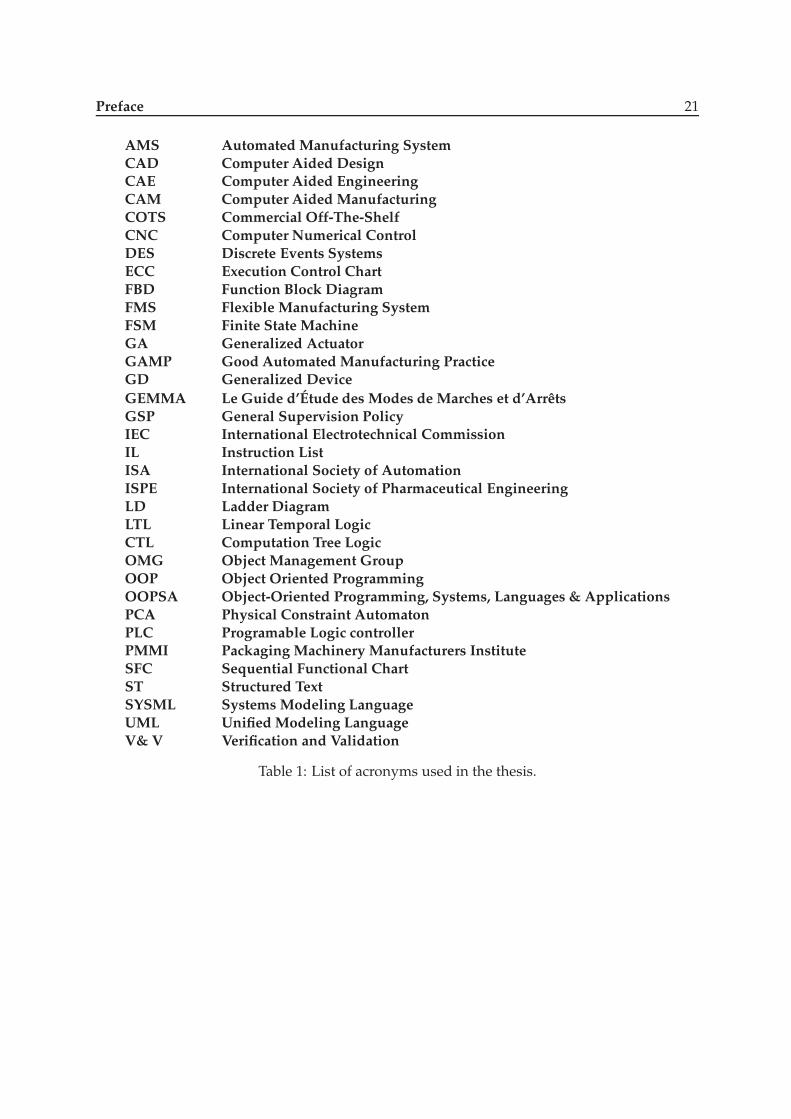
AMS Automated Manufacturing SystemCAD Computer Aided DesignCAE Computer Aided EngineeringCAM Computer Aided ManufacturingCOTS Commercial Off-The-ShelfCNC Computer Numerical ControlDES Discrete Events SystemsECC Execution Control ChartFBD Function Block DiagramFMS Flexible Manufacturing SystemFSM Finite State MachineGA Generalized ActuatorGAMP Good Automated Manufacturing PracticeGD Generalized DeviceGEMMA Le Guide d’Étude des Modes de Marches et d’ArrêtsGSP General Supervision PolicyIEC International Electrotechnical CommissionIL Instruction ListISA International Society of AutomationISPE International Society of Pharmaceutical EngineeringLD Ladder DiagramLTL Linear Temporal LogicCTL Computation Tree LogicOMG Object Management GroupOOP Object Oriented ProgrammingOOPSA Object-Oriented Programming, Systems, Languages & ApplicationsPCA Physical Constraint AutomatonPLC Programable Logic controllerPMMI Packaging Machinery Manufacturers InstituteSFC Sequential Functional ChartST Structured TextSYSML Systems Modeling LanguageUML Unified Modeling LanguageV& V Verification and Validation
Table 1: List of acronyms used in the thesis.

22 Preface

Chapter 1Control design in industrial automatedsystems
This chapter showes the main characteristic of modern industrial auto-mated systems. In last years there was a growth in the automation ofproduction lines, implying the use of systems that are required to beever more performing, reliable, flexible but at a lower price. Machinesare then increasingly filled with embedded components constituted byengines, integrated in the mechanics, managed through a specific soft-ware command. The number and types of embedded components andtechnologies enabling specific functions (i.e. motion control, failure anal-ysis, monitoring etc.) has raised the level of complexity of the wholesystems with a clear impact on design process, that becomes a complextask, in which different technological fields interact (i.e. competences inmechanical engineering, in electronic engineering, in software and con-trol engineering are needed to fulfil these tasks).
1.1 Design specification in industrial automated system
The enlarged demand of innovative and technologically advanced solutions in all industrialapplication domains has in recent years strongly promoted the development of powerful andversatile Automated Manufacturing Systems (AMSs), capable of working more reliably, withan increased product processing accuracy, and at a faster, sometimes astonishing, speed. Theenhanced functionalities and overall performance characterizing the modern AMSs are, doubt-less, primarily attributable to the novel ideas and effective solutions purposely conceived bythe designers of their mechanical structure. In the achievement of these goals, however, alsothe design of the AMS control system plays a crucial role, because of the always more relevantand wider spectrum of activities delegated to it. Besides the automation of working cycles,other essential requirements that the control system is asked to deal with typically concern theneed of:
23

24 Control design in industrial automated systems
(a) Centralized architecture. (b) Decentralized architecture. (c) Distributed architecture.
Figure 1.1: Control systems architecture evolution.
• emulate the behaviour of manifold mechanical devices (e.g., cams, gear wheels, etc.),so as to reduce the system structural complexity and limit downtimes due to automaticchangeover of its constituent parts;
• dynamically adapt the control strategies according to different productive requirementsand operational scenarios;
• ensure high quality of the finished product, making a thorough verification of its process-ing correctness while preventing useless workings and wastage of raw materials;
• support the operator with timely and precise indications about the actions that shouldbe undertaken to establish or restore the desired operating conditions, ridding him ofhazardous or burdensome jobs;
• provide a comprehensive set of real-time diagnostics information and pre-processed pro-duction data, adequately supporting system maintenance, raw materials and finishedproducts handling, production organization and planning.
Such a broad set of functional requirements highlights and common experience makes it ev-ident, that the design of the control system of a complex AMS is undoubtedly a hard task,involving a multidisciplinary cultural background [85]. Different considerations, however,should be pointed out as regards hardware and software design. From the former viewpoint,designers can profitably rely on technologically advanced commercial-off-the-shelf (COTS) re-sources, as powerful processing units, special-purpose controllers, smart I/O devices, network-ing infrastructures, which can be modularly composed to build up quite sophisticated and scal-able architectures conforming to the application needs.
The hardware architectures of automated systems during last decades, like it’s possible tosee in figure 1.1, it’s developed through different architectures. Centralized architectures (seefig. 1.1(a)), typically based on programmable logic controllers (PLCs) equipped with simpleoperator panels and supported in the accomplishment of complex or time-constrained tasksby special-purpose smart units (such as electrical axes controllers, simple HMI panale, ecc.),have dominated the hardware architecture up to the 80’s. In the next decade, the spreading ofdecentralized architectures (see fig. 1.1(b)) is strongly promoted by the advent of the field-bustechnology and by the use of industrial PC as a means to provide highly complex and expensivemachines with definitely more user-friendly human-machine interfaces (HMIs). The ensuing

1.2. Classification of industrial automated systems 25
!"#$
''$''$
!"#$
''$''$
Motion Control
Human Machine Interface
Motion Control
Control Logic
Distributed I/O, Real-Time, Task handling
Figure 1.2: Control system architecture in automated systems.
availability of powerful multi-core PC-embedded systems, suitably enriched with soft-PLC en-vironments and natively fitted out with the facilities needed for network interoperability, notonly leads to the integration of both the control and HMI functionalities within a single plat-form, but also discloses the way towards fully distributed architectures (see fig. 1.1(c)). Theoverall automated system becomes not only a single machine but complex more different ma-chine working together in a production lines.Unfortunately, plain applicability of the “buy, plug & play” principle continues to have a nar-rower scope when the design of the control system from the software viewpoint is considered.The kind of facilities that designers can directly find on the market, in terms of COTS soft-ware component libraries, networking-oriented middleware, development tools and run-timeenvironments, provide in fact an adequate support as regard the implementation of either top-level or bottom-level functionalities, typically pertaining to the domains of user-friendly HMIs,closed-loop regulation and motion control, fieldbus-based interconnection of remote smart de-vices. This functionalities are represented in figure 1.2, in a hierarchical representation wherein the top level are presented the functionalities to interface the machine with the operator,and in the bottom level are presented the field functionalities. In the middle is presented thecontrol logic of the automated system, for this part of control of the entire machine there arenot availability and usually in this part is inserted the basic control of the machine during thenominal condition and all the diagnosis algorithms of fault detection. The “huge hole” exist-ing in the middle needs to be properly filled in by software designers, still missing concretesupport from vendors of industrial automation technologies as regards generally applicableframeworks, or at least application-level design patterns (in 2.2 wil be present a definition ofdesign pattern), that can be profitably exploited (or assumed as reference guidelines) in theprocess of organizing and structuring the control logic of AMSs.
1.2 Classification of industrial automated systems
To better understand what are industrial automated systems and their complexity from a pointof view of their mechanical architecture and control logic architecture it’s possible to classifyindustrial automated systems based on its function and by the form of material handling sys-

26 Control design in industrial automated systems
(a) An example of assembly machine. (b) An example of testing machine.
Figure 1.3: Example of industrial automated machine.
tem. There are a wide number of functions that a machine can perform, but if one looks at thehistory of what has been built to date, and one was to try to classify the significant groupingsthat would result, several major classifications are:
• Assembly machines;
• Inspection machines;
• Test machines;
• Packaging machines;
• Computer numerical control (CNC) machines;
• Production processes.
This classification wants only try to defined different kind of automatic machine, of curse incomplex production line we can found a mix of this machine.
1.2.1 Assembly machines
Assembly Machines as a group can range from the production of a high-volume part such asa spark plug or a piece of home kitchen cabinet hardware, to the construction of a cell phone.Throughput rates and product flexibility expectations can vary and usually changeover is re-quired. Figure 1.3(a) shows a generic assembly machine, a robot that assembles short-strokecylinders. There is the base part of the product brought into the workcell in some fashion.Parts feeders are used for the components to be added to the base part. And another methodof transferring out the completed assembly is usually required. If the assembled part is a hingefor your home kitchen cabinets, then the output could be simply dumping them into a bin.

1.2. Classification of industrial automated systems 27
1.2.2 Inspection machines
Although in-process inspection is currently desired even more, inspection is often performed asan integral operation within the assembly machine. Computer vision systems and dimensionalmeasurements are two of the commonly found inspections performed within the assemblymachine. However, stand-alone inspection machines for checking a packaged product for thecorrect weight (check-weighers) and making sure no metal filing from all of the food processingmachines fall into your box of corn flakes (metal detectors) do exist and have meaningful nichemarkets. Most of these inspection machines generically have a product inflow, a checkingstation, and two outflows. One of these outflows is the good product and the other outflowis for defective products. Depending on the product and its defect, the defective product maystill be sold. If it is a food product and is only underweight, it can be eaten, possibly showingup in a factory seconds store. Obviously, products with metal filings are recycled, burned forheat value, or thrown away. Some examples of inspection process are:
• Checking one or more dimensions with mechanical gauging or electrical sensor;
• Checking one or more dimensions or features using a vision system;
• Checking weight for correct amount;
• Checking a liquid’s volume by weight or level;
• Checking a filled Stand up Pouch (SUP) for leaks;
• Checking a product for metal filings, etc.;
• Checking free prize inside a box product.
The results from all of these can range from health risks (metal filings) to disappointed cus-tomers like a missing free prize. If we consider a production line to product wine bottle, ofcourse the quality of wine bottle is depending from wine and bottling process, but from cus-tomer point of view and not perfect label alignment is a index of low quality of the wine bottle.An example of inspection machine is shown in figure 1.3(b), the machine test the colour of theworkpiece and its height to decide if to works or not the workpiece.
1.2.3 Test machines
Machines that conduct some performance check on the filled, assembled, or processed productare sometimes referred to as test machines. Although some might argue that testing is part ofinspection, the distinguishing feature is often the cycling of the product in some or all of itsdesigned operation. In other words, an inspection machine functions by either a noncontactmode, or with a simple contact where some measurement or property is determined. A testmachine makes the product do some action or work, such as cycling a spray head from a hand-powered misting bottle. The test is carried out on either a random basis, or on every sprayhead if trouble has been observed in the past, but the spray head is either passed as workingproperly, or is rejected. As opposed to inspection machines being potentially integrated into anassembly machine, most test machines are separate from the assembly process. Test machinesare often highly specialized to the product being assembled or processed, and the devices usedto perform the test and to judge the results cannot be easily integrated into the other machines.Figure 4.3 shows a test machine that is checking the previously assembled widget to see if itwill hold together or whether it will fall apart. Following the example of testing the spray head,

28 Control design in industrial automated systems
there would need to be devices to move a single spray head into the test station in the correctorientation, an actuator to perform the test, a device to advance spray heads that pass the test,and another device to dump a rejected spray head into a hopper. The controller may need tobe smart enough to allow the spray head to be actuated a variable number of times, so as notto reject heads that are good but not the best performers.
1.2.4 Packaging machines
Any finished consumer product of any value gets packaged in one of many different types ofpackages. It can be bags, boxes, cartons, aseptic boxes etc.. None of these packages significantlyimproves the performance of the product inside, but the packaging does help the consumerunderstand the product, differentiate the product from the competition, and improve salesdramatically. The area of packaging results quite large some typical packaging machines aremachines devote to:
• Closing filled corrugated cardboard boxes;
• Filling bottles with liquids;
• Filling bags with dry products;
• Placing products into cartons;
• Weighing products for accuracy;
• Metal detection for safe consumption by consumer.
As it’s to note the last two machines have been discussed in the previous section, this factdepend that it’s not possible to have a complete division from machines and a complex pro-duction line is a composition of different kind of machine. To understand how is importantpackaging machine, we can think about how many product from packaging machine are inour daily life. Every day most of us use bottles filled with liquids, buy product in box like bis-cuits or cigarets, so there is a very large number and different kind of manufacturing machine.
1.2.5 Computer numerical control machines
Computer numerical control refers to the automation of machine tools that are operated byabstractly programmed commands encoded on a storage medium, as opposed to manuallycontrolled via handwheels or levers, or mechanically automated via cams alone. The first CNCmachines were built in the 1940s and ’50s, based on existing tools that were modified withmotors that moved the controls to follow points fed into the system on paper tape. Theseearly servomechanisms were rapidly augmented with analog and digital computers, creatingthe modern computer numerical controlled machine tools that have revolutionized the designprocess. In modern CNC systems, end-to-end component design is highly automated usingCAD/CAM programs. The programs produce a computer file that is interpreted to extract thecommands needed to operate a particular machine, and then loaded into the CNC machinesfor production. Since any particular component might require the use of a number of differenttools (as drills, saws, etc.) modern machines often combine multiple tools into a single “cell”.In other cases, a number of different machines are used with an external controller and hu-man or robotic operators that move the component from machine to machine. In either case,the complex series of steps needed to produce any part is highly automated and produces a

1.2. Classification of industrial automated systems 29
Figure 1.4: Example of a classic CNC machine.
part that closely matches the original CAD design. In figure 1.4 an example of a classic CNCmachine.
1.2.6 Production Processes
Production processes are procedures involving chemical or mechanical steps to aid in the man-ufacture of an item or items, usually carried out on a very large scale. Most processes make theproduction of an otherwise rare material vastly cheaper in price, thus changing it into a com-modity; i.e. the process makes it economically feasible for society to use the material on a largescales, in machinery, or a substantial amount of raw materials, in comparison to batch or craftprocesses. Production of a specific material may involve more than one type of process. Typ-ical examples of production processes are chemical process, like in figure 1.5 where is shownan example of a gasification process, pharmaceutical process, industrial heavy etc. Productionprocess can be roughly categorized as one of three types: batch, continuos, and discrete.
Batch Processes this kind of process are characterized by generation of finite quantities of ma-terial, called a batch, at each production cycle. Material is produced by subjecting specificquantities of input materials to a specified order of processing actions using one or morepieces of equipment. The batch goes through discrete and different steps as it is trans-formed from raw materials, to intermediates, and to final materials. Processed materialis often moved, in total, between different vessels for different processing steps. Con-trol of batch processes is not discrete or continuous, but it has the characteristics of both.Many pharmaceutical, specialty chemical, food, and consumer packaged goods are batchprocesses. They may be batch processes because the underlying chemistry or physicscan only be done on all the material at once. Some batch processes are defined as batch

30 Control design in industrial automated systems
Biomass
Temperature Control
Gas Reactor
Figure 1.5: Example of production process machine for a gasification process.
because there are more product types than production lines, and each production linemust be able to produce several different products. This is common in electronics, semi-conductors, food processing, consumer products, and specialty chemical production. Forexample, the same production equipment may produce batches of chocolate cookies inthe morning and sugar cookies in the afternoon.
Continuos Processes this kind of processes are characterized by the production of materialin a continuous flow. Continuous processes deal with materials that are measured byweight or volume, without a discrete identity for any part of the produced material. Ma-terials pass through different pieces of specialized equipment, each piece operating in asteady state and performing one dedicated part of the complete process. Once running ina steady state, the process is not dependent on the length of time it operates. Many bulkchemicals are produced in continuous production systems. Startup, transition, and shut-down do not usually contribute to achieving the desired processing. Material producedduring these times often does not meet end product quality specifications and must behandled separately. Startup, transition, and shutdown, however, are important eventsthat require specific procedures to be followed for safe and efficient operations.
Discrete Processes Discrete processes are characterized by production of a specific quantity ofmaterial, where each element of the material can be uniquely identified. Discrete pro-cesses deal with material that is counted, or could be counted. In discrete processes, aspecified quantity of material (maybe just one element) moves as an entity between dif-ferent pieces of processing equipment. The assembly of computer circuit boards is anexample of a discrete process. Usually, multiple elements are processed using the sameequipment configuration and raw materials. Startup, transition, and shutdown often pro-duce the desired end product. Startup, transition, and shutdown are usually tightly con-trolled because they significantly impact the overall equipment efficiency. These eventsrequire specific procedures to be followed to place production equipment in the rightstate to make the desired product.
A widen discussion and description of production process can be found in [15].

1.3. Conclusions 31
1.3 Conclusions
In chapter was presented an introduction of industrial automated systems. In section 1.1 a briefdescription of most important specification and task of an automated systems are reported andit was presented some easy and typical example to understand what are automated systems.Starting from this typical example a functionality characterization was presented, an interest-ing reader can found more information in [22],[91] [15]. A particular consideration is has tofocus on packaging machine, to understand its importance the consortium of machine pro-ducers, is called Packaging Machinery Manufacturers Institute (PMMI) has estimated around350 types of packing machine (see [22] and www.packexpo.com). Also in Italy are presenteda large number of packaging machine industry, in particular a great concentration of industryis located around Bologna area; for this reason the area around Bologna is called “packagingvalley”.From this brief introduction is clear how automated systems and in particular manufacturingsystems are very complex systems, of sure the “success” of an automated industrial system,in terms of functionalities and performances, are strongly relies on its physical structure: i.e.on the choices made during design phase in terms of the mechanical structure and electricalelectronic architecture, but how discussed in 1.1 the control system plays a key role for theachievement of the targeted performance. The aim of this thesis is define an architectures forthe modern industrial automated systems to help the designer to design the control system.

32 Control design in industrial automated systems

Chapter 2State of the art of software engineering inindustrial automated systems
This chapter deals with an overview of the control design in indus-trial automated systems and how the modern software engineering tec-quiniques, like object orienting programming, are applied to modern in-dustrial automated systems.
2.1 Software architecture in industrial automation
As explained in the chapter before an automated manufactory system is a machine that per-forms autonomously an industrial process, in which materials and energy are transformed toproduce either consumer goods or input to other manufacturing systems. The task of con-trol design for manufacturing systems represent a challenging and interesting problem, sincethe application domain presents heterogeneous and requires engineering efforts that includedifferent kind of technological skills. In fact, the development process of a manufacturing ma-chine control system is composed of several sub-tasks in the field of mechanical engineering,electric/electronic engineering, systems theory and also computer science, as the whole sys-tems is composed by mechanical parts for product handling, heterogenous sensors and actua-tors for motion control and overall supervision, and several special on general purpose digitalcontrollers that must be adequately programmed to perform efficiently the control algorithms.One of the most important control hardware in industrial automation filed are Programmablelogic controller (PLC). PLC or programmable controller is a digital computer used for automa-tion of electromechanical processes,such as control of machinery on factory assembly lines,amusement rides, or lighting fixtures. PLCs are used in many industries and machines. Un-like general-purpose computers, the PLC is designed for multiple inputs and output arrange-ments, extended temperature ranges, immunity to electrical noise, and resistance to vibrationand impact. Programs to control machine operation are typically stored in battery-backed ornon-volatile memory. A PLC is an example of a real time system since output results must be
33

34 State of the art of software engineering in industrial automated systems
produced in response to input conditions within a bounded time, otherwise unintended oper-ation will result. The PLC was invented in response to the needs of the American automotivemanufacturing industry. Programmable logic controllers were initially adopted by the auto-motive industry where software revision replaced the re-wiring of hard-wired control panelswhen production models changed. Before the PLC, control, sequencing, and safety interlocklogic for manufacturing automobiles was accomplished using hundreds or thousands of re-lays, cam timers, and drum sequencers and dedicated closed-loop controllers. The process forupdating such facilities for the yearly model change-over was very time consuming and expen-sive, as electricians needed to individually rewire each and every relay (a complete descriptionof PLC can be find in [7]).As it is common practice in every engineering context dealing with complex systems, softwaredesigners tackle the problem relying on the “divide et impera” approach. Drawing inspira-tion from the fundamental principles of decomposition and abstraction, they proceed to par-tition the whole AMS control logic into manageable simpler components, usually organizedaccording to a hierarchical multi-layer architecture that directly mirrors, at least to a certain ex-tent, the mechanical structure and the sensorial-actuation equipment of the AMS itself. Manyfactors, however, often hinder software designers from targeting the decomposition processtowards the definition of an architecture comprising a wide variety of modular and reusablecomponents, as much as possible platform-independent and directly applicable in other sim-ilar contexts. Among the common claimed (some arguably) factors causing software designto be more adherent to the code-and-fix approach rather than properly focussed in the prob-lem domain, the following ones seem generally the most relevant. First of all, the ancillaryrole attributed to the software designers activity, too often addressed at the implementation ofquickly-operative vehicles used for experimentally ascertaining the validity and effectivenessof the choices made by the AMS mechanical and electrical design team. Secondly, the burden ofcompelling, sometimes inappropriate, time-to-delivery commitments, which not only precludeany form of brain storming and exchange of significant experience among software designers,but often direct them to take approaches targeted at application-specific objectives only. Fi-nally, the limited expressive power of (most of) programming languages currently available forPLC-based or soft-PLC PC-based platforms, somehow precluding plain applicability of well-established principles and methodologies proper of the object-oriented design paradigm.It is therefore not entirely surprising that the costs associated with the software developmentlifecycle generally grow well beyond the budgeted expectations. In order to help solve theseproblems, many interesting proposals have been recently reported in the scientific and techni-cal literature. Among them, some (e.g., mechatronic approaches) aim at improving the cost-effectiveness of the overall design process, favoring and stimulating concurrent engineering,co-design and co-simulation. Others suggest the use of state-of-the-art modelling languages(e.g., UML) and automatic code generation tools to enhance the software design, developmentand maintenance process. Several propose formal models (e.g. compositional theories, model-checking, model extraction) or techniques for verification and validation of component soft-ware, as a viable means to enforce reliability and reduce debugging efforts. Particularly impor-tant is also the contribution of renowned International Committees and Organizations, pavingthe way towards a standardization of the design methodologies (e.g. the IEC 61131/61499norms, the Model Driven Architecture, MDA, proposal). The work here referred takes thecue from the ascertainment that an effective solution to the mentioned problems cannot derivesolely from a fully synergistic cooperation between all design team’s members, as well as fromthe use of powerful CAD-CAE tools and integrated development environments. This work tryto define a generally-applicable design patterns focussing on cross-cutting control logic func-

2.2. Design patterns in industrial automation 35
tionalities and suitably abstracting from application-specific details, may support the processof modelling, structuring and implementing highly modular and reusable components.
2.2 Design patterns in industrial automation
The aim of this thesis is define a design pattern for industrial automated systems, so it is impor-tant to understand what design patterns are, and what they mean. A pattern can be variouslydescribed as:
• a practice or a customary way of operation or behavior.
• a model considered worthy of imitation.
• a blueprint intended as a guide for making something.
All of these descriptions apply to design patterns. A design pattern is a blueprint intendedas a guide for use in design processes. Specifically in the field of software engineering andprogramming, a design pattern is a repeatable solution to a commonly occurring problem. Adesign pattern is not a design. Instead, a design pattern is a template for how to solve complexproblems that applies to different, but related, situations. A design pattern can be transformeddirectly into code. Design patterns exist in many areas, from architecture and construction, tosoftware design and development.
• In architecture, there are design patterns in houses. For example, colonial-style houseshave the same first and second floor layout, varying in details and size, but not in overallstructure.
• In civil engineering, suspension bridges follow design patterns, varying in scale and de-tails, but not in overall structure.
• In software engineering, computer-human interfaces follow design patterns for windowsand mouse actions, varying in detail for each application, but not in overall structure.
• Novels and plays follow design patterns, such as a typical mystery or romance novel plot.
Design patterns are used everywhere in modern society. They allow us to reuse the knowledgeand experience of others. Design patterns mean that we do not have to solve every problemfrom first principles, but can instead rely on the experience of others who have come up withreusable solutions. Design patterns are usually developed as solutions to problems that can bereapplied to related problems. The term design pattern was first defined by an architect Christo-pher Alexander. His book (see [3]) related to urban planning and building architectures. Heclaimed that the architectural and engineering methods did not fulfil the real demands of theusers of the buildings and urban environment. In its work, Alexander explained that there wassome uniform way of building houses and towns that were comfortable and suit for the users’need. Alexander defines the pattern language, a common language that is shared by the archi-tects to define the patterns that occur repeatedly during the design of buildings. This languageshould not be confused with programming languages. It is merely a common vocabulary andsemantics for architects to speak about best-practice designs that solve a common problems.There are several one sentence definitions of patterns by various authors, one used by Alexan-der is:

36 State of the art of software engineering in industrial automated systems
Each pattern describes a problem which occurs over and over again in our environment, and then de-scribes the core of the solution to that problem, in such way that you can use that solution a million timesover, without ever doing it the same way twiceIn 1987 Kent Beck and Ward Cunningham began experimenting with the idea of applying pat-terns to programming at OOPSLA (Object-Oriented Programming, Systems, Languages & Ap-plications) [5], they used the Alexander’s idea in Smalltalk programming Tektronix. The sameidea was applied later by Erich Gamma to study the reuse of Object-Oriented software (see[36]). In software engineering, a design pattern is a general reusable solution to a commonlyoccurring problem in software design. A design pattern is not a finished design that can betransformed directly into code. It is a description or template for how to solve a problem thatcan be used in many different situations. Object-oriented design patterns typically show rela-tionships and interactions between classes or objects, without specifying the final applicationclasses or objects that are involved. Design patterns reside in the domain of modules and inter-connections. At a higher level there are Architectural patterns that are larger in scope, usuallydescribing an overall pattern followed by an entire system. Not all software patterns are designpatterns. For instance, algorithms solve computational problems rather than software designproblems.In industrial automated systems, automation patterns have been applied mainly in softwareengineering problems of the automation systems. This is due to the origins of patterns inobject-oriented software engineering. In general, in an object-oriented automation softwarethe patterns proposed by E. Gamma ([36]) should be applicable. These patterns are genericin object-oriented programming, and the context of industrial automation does not make anexception. Automation systems are, however, a bit different from other information process-ing systems. The context of industrial automation, or the application domain, has a dynamicand changing nature of the system configuration, high data intensity, real-time constraints ofmeasurements and control as well as the heterogeneity of the systems in a production plant.Somewhat similar environments could be found from telecommunication networks, and there-fore the design patterns could be thought to be similar. An example to describe an automationpattern i using formal and informal diagrams, the formal notation uses UML notation. UML isthe Unified Modelling Language (see [66], [67] and [77]). UML defines a rich set of diagramsand methods for describing complex systems and complex system solutions. In next sectionswe will see different design patterns for industrial automated systems.
2.2.1 A design pattern for control process - S88
A first example of design patterns for automated systems is the standard ANSI/ISA 88 (calledS88). S88 is a standard addressing batch process control, it is a design philosophy for describingequipment, and procedures. It was approved by the ISA in 1995 and it was adopted by the IECin 1997 as IEC 61512-11.S88 provided for the first time a well thought-out approach to flexible manufacturing that wasaccepted by automation, control, and process engineers. It is a consistent set of standards andterminology for batch control and defines the physical model, procedures, and recipes. Thestandard sought to address the following problems: lack of a universal model for batch control,difficulty in communicating user requirement, integration among batch automation suppliers,difficulty in batch control configuration. The first step of a process-automation project is to de-fine the requirements, usually they are defined by functional specification to try to design the
1The official standard is ANSI/ISA-88.01-1995. Batch control Part 1: Models and terminology. The internationalequivalent is IEC 61512-1.

2.2. Design patterns in industrial automation 37
systems with a modular approach. A functional specification defines what the system shoulddo, and what functions and facilities are to be provided. The GAMP (Good Automated Man-ufacturing Practice), a trademark of the International Society of Pharmaceutical Engineering(ISPE) describes a set of principles and procedures that help ensure that the product have therequired quality. One of the core principles of GAMP is that quality cannot be tested into abatch of product but must be built into each stage of the manufacturing process (for a moreexhaustive definition the reader is refereed to [37] [51]). For this reason it is important to havemodular approach to design the entire systems (control logic, mechanical structure etc.).The S88 standard try to define a sort of architecture separating the product definition informa-tion from production equipment capability. This separation wants define a procedure whichallows same equipment can be use in different ways to make multiple products, or differentequipment can be to be use to produce the same product. Product definition information iscontained in recipes, and the production equipment capability is described using a hierarchicalequipment model. This choice for the recipe/equipment separation is to try to make recipedevelopment simple enough to be accomplished without requiring the services of a controlsystems engineer.The recipe phase does not specify how the action is performed, the recipe only under whatcondition the phase is to be executed. S88 define 4 types of recipe but the most importantare master and control recipes: master recipes are the templates used to create control recipeswhile control recipes are executed to produce a batch. The master recipe may specify informa-tion such as what types of equipment will be used, or what types of materials will be used. Thecontrol recipe has information added for the specific batch, such as what batch ID to assign tothe batch, what material lot ID to assign to the produced material, and what equipment to usein production of the batch. The organization structure for equipment is called the equipmenthierarchy. The S88 for the equipment hierarchy starts at the corporate level, called an enter-prise in the standard and it arrives up to the production unit (to a complete definition see [49],and [50]). Equipment modules use equipment procedural control to achieve minor processingtasks. An equipment module is the container for performing the different elements of proce-dural logic required to achieve the process task. Equipment modules may be contained withinunits, or may be shared between units in a process cell. In either case, they usually containall of the physical equipment and control capabilities to perform their minor processing func-tion. The purpose of an equipment module is to coordinate and execute the procedural logicrequired to implement a phase, or to execute any other required equipment procedural control.The S88 try to standardize how the different actions, the recipes, are executed defining the ex-ecution states. In the S88 the execution state is called procedure’s state. The standard don notdefine all the states but it provides an example set of states but not establish a formal standard,an example of procedural control state is depicted in figure 2.1(a). The states usually have thissignification:
Idle: The procedure element is available for execution.
Running: The procedure element has received a start command and is running its procedurallogic.
Complete: The procedural element has completed normally.
Holding: The procedural element has received a hold command and is in the process of goingto a stable held state. The procedural element may transition directly to held state, if nospecial actions are required.

38 State of the art of software engineering in industrial automated systems
(a) State model procedural control.
MANUAL
SEMIAUTOMATIC
Manual
AUTOMATIC
Semi
Manual
Auto
Auto Semi
(b) State model element modes.
Figure 2.1: Example of S88 design pattern.
Held: The procedural element is in a state suitable for a longterm delay that may be resumedlater.
Restarting: The procedural element is performing any restart logic required to go from a heldstate to a running state. The procedural element may transition directly to running state,if no special actions are required, then .
Stopping: The procedural element has received a stop command and is transitioning to astopped state as a controlled normal stop. The procedural element may transition di-rectly to stopped state, if no special actions are required.
Stopped: The procedural element is no longer running and has performed a controlled normalstop.
Aborting: The procedural has received an abnormal stop (abort command) and is executingany aborting logic. The procedural element may transition directly to aborted state, if nospecial actions are required.
Aborted: The procedural element is no longer running and has performed an abnormal stop.
The states of machine of figure 2.1(a) evolves under the commands:
Start : Starts the procedural element. Used by an operator to start a control recipe, the logic inthe procedure takes care of starting the lower-level elements.
Hold: Commands the procedural logic to go to a held state. Usually used by an operator topause operation of the procedure logic.
Restart: Commands the procedure logic to release the hold and return to the running state.
Stop: Commands the procedure logic to stop executing and perform a normal shutdown.
Abort: Commands the procedure logic to stop executing and perform an abnormal shutdown.
Reset: Commands the procedural logic to reset and be ready to execute again. This commandis usually performed by the recipe-execution system and is automatically sent after thesystem determines that the procedure element has completed.

2.2. Design patterns in industrial automation 39
S88 try to standardize also a “mode of operation”. The mode determines how procedural ele-ments respond to commands and how procedural control progresses. The modes can be rep-resented in a state model as depicted in figure 2.1(b), this is an independent state model fromthe procedural element states. The mode defines what a recipe-execution system does withtransitions between procedure steps. In automatic mode, the procedure logic is automaticallyexecuted. In manual mode, the operator determines what logic to perform. In semiautomaticmode, the operator decides when to step the logic.While the ISA 88 standard has been applied to many non batch problems, the is no consistentlydefined methods for applying it in non stop-production. Non stop production is either contin-uos or discrete manufacturing where there are no breaks allowed in the product flow. Discreteproduction examples include the movement of discrete products , such as bottles, electroniccomponents etc. Continuos production occurs when the product moves in a a flow there areno discrete countable elements a typical example are chemical production. To extend the S88 ofthis kind of process, a set of rules was defined to apply S88. This set of rules is called NS88, thegoal of this approach is to maintain the concepts of separation of product definition, the recipesfrom intrinsic equipment capabilities. For a complete definition of this approach the reader isreferred to [15].
2.2.2 A design pattern for manufacturing systems - GEMMA
Another example of design pattern is GEMMA (Le Guide d’Étude des Modes de Marches etd’Arrêts.), it means literally design guide for start and stop modes. GEMMA is a graphicalchecklist which allows the designer to define from the beginning all the operations and theirconsequences for a machine. The goal of Gemma is help the designer to define all the possiblemachine situation during its working and managing all the fault and emergency situation.GEMMA is a graphical tool and it borns as an helper to define a SFC project with a well-definestructure. GEMMA is baed on three basic concepts: (i) Start modes are defined with the controlpart fully energized, (ii) The definition of production state (iii) Three general types of start andstop modes.For GEMMA, the definition of start and stop modes affects the whole production and controlparts of the machine, but from a control point of view, with the control part fully energized andi n working order. Basically, we can define two general modes: control part not energized andcontrol part energized. The system, comprised of the machine and its control, will be in onlyone of those two states and can switch from one state t o the other through transitions. Startmodes are defined with the control part fully energized. Any machine can be broken downinto a productive part and a control part. Materials and energy are supplied to an automationproduction system, which produces transformed materials in accordance with the operator’sorders and the environment. The production state is referred to a set state where the machineproduces some work which adds value to materials which are fed into it; this is the addedvalue. However, a machine is not 100% of the time in the production mode; it could be, forexample, under repair, adjustment or modification. Three general types of start and stop modes aredefined in GEMMA, in these three “ways” are groped all the different modes of the machinehave been defined as:
Production Procedures: These include all necessary modes used too obtain the added valueexpected for the machine; they are not necessarily all productive modes (preparationmode) but are indispensable for production (before, during or after production).
Stop Procedures: A machine i s never operated 100% of its full useful life, so it is stopped it f

40 State of the art of software engineering in industrial automated systems
o r external reasons (end of the work period, lack of supply).
Failure Procedures: Any machine or system fails at one moment or another. These circum-stances are described in the failure procedures, which cover all the internal reasons forstopping the machine. NOTE: The description of the states includes actions or states ofany part of the machine, including the control part; it can also include special action to betaken by the operator or maintenance people themselves, such as manual action on themechanisms, or writing in a log book, or reference to external written procedures, amongothers.
In figure 2.2 is depicted the model architecture of GEMMA where are emphasize the three typesof start and stop, in the following a brief description of the three states groups:
Production ProceduresF1 Normal Production: This is the normal mode of production of the machine which,in this state, produces the transformed materials as the main and expected output of themachine.F2 Start up: This state i s used for the machines which request special action, such aspreheating, pressurization, prefilling or other, prior to production.F3 Shut down: Some machines need to be emptied and cleaned before stopping or be-tween production cycles.F4 Unsequenced Test Mode: this mode allows the operation of some parts of the ma-chine to be checked without following the usual sequence of operation. More commonly,this state can be called “human” control.F5 Sequenced test mode: In this mode, the machine’s cycle of operation can be followedstep by step in the normal sequence. The machine can or cannot produce during thisstate.F6 CALIBRATION MODE: This mode allows the instruments installed on the machineto be adjusted, set, calibrated or recalibrated.
Stop ProceduresA1 Initial State Stop: This corresponds to the zero energy state, with the machine de-energized but with the control circuits energized. Exist a clear relationship with GRAFCETinitial state stop.A2 Requested Stop at the End of Cycle: In this mode, the machine has been asked tostop at the end of the normal production cycle, i.e. to go into the A1 state, but productionmust be completed before then. A2 is a transient mode to A1.A3 Requested stop in a determined state: The machine has been asked to continue pro-duction before stopping at a state other than the end of the production cycle. This atrancient state before A4.Obtained stop: The machine i s stopped in a step other than the normal cycle’s final po-sition of the normal cycle.A5 Preparation to Restart after a Failure: In this mode, all the requested actions (ma-terial, clearing, cleaning, change of broken tool, etc.) after a failure are effected beforerestarting.A6 Production Reset to the Initial State: In this mode, the machine or its mechanismis set back, manually or automatically, to a position ready for resumption of productionfrom the initial state.
Failure ProceduresD1 Emergency Stop: This mode regroups all the special sequences or actions which have
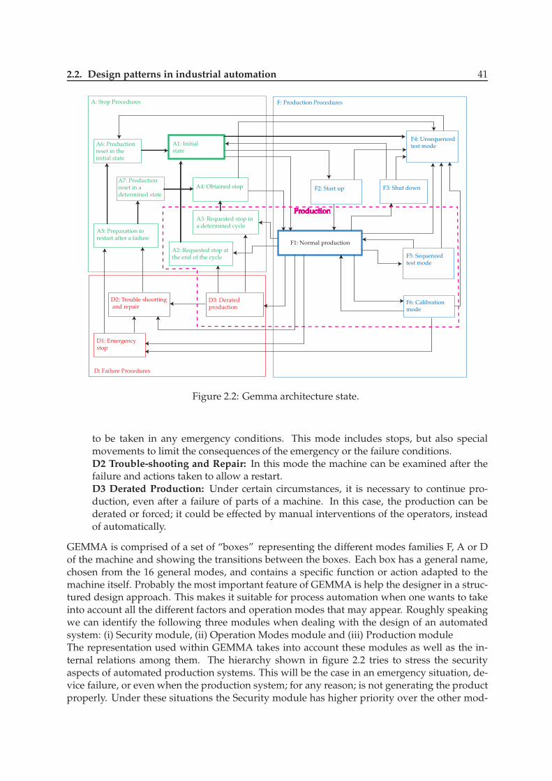
2.2. Design patterns in industrial automation 41
A6: Productionreset in theinitial state
A1: Initialstate
A7: Productionreset in adetermined state
A5: Preparation torestart after a failure
A4: Obtained stop
A3: Requested stop ina determined cycle
A2: Requested stop at the end of the cycle
F2: Start up
F1: Normal production
F3: Shut down
F4: Unsequenced test mode
F5: Sequenced test mode
F6: Calibration mode
D2: Trouble shootting and repair
D1: Emergency stop
D3: Derated production
A: Stop Procedures F: Production Procedures
D: Failure Procedures
Figure 2.2: Gemma architecture state.
to be taken in any emergency conditions. This mode includes stops, but also specialmovements to limit the consequences of the emergency or the failure conditions.D2 Trouble-shooting and Repair: In this mode the machine can be examined after thefailure and actions taken to allow a restart.D3 Derated Production: Under certain circumstances, it is necessary to continue pro-duction, even after a failure of parts of a machine. In this case, the production can bederated or forced; it could be effected by manual interventions of the operators, insteadof automatically.
GEMMA is comprised of a set of “boxes” representing the different modes families F, A or Dof the machine and showing the transitions between the boxes. Each box has a general name,chosen from the 16 general modes, and contains a specific function or action adapted to themachine itself. Probably the most important feature of GEMMA is help the designer in a struc-tured design approach. This makes it suitable for process automation when one wants to takeinto account all the different factors and operation modes that may appear. Roughly speakingwe can identify the following three modules when dealing with the design of an automatedsystem: (i) Security module, (ii) Operation Modes module and (iii) Production moduleThe representation used within GEMMA takes into account these modules as well as the in-ternal relations among them. The hierarchy shown in figure 2.2 tries to stress the securityaspects of automated production systems. This will be the case in an emergency situation, de-vice failure, or even when the production system; for any reason; is not generating the productproperly. Under these situations the Security module has higher priority over the other mod-

42 State of the art of software engineering in industrial automated systems
ules in order to take the appropriate decision. It is also worth to notice the introduction of theoperator as an integral part of the system. The operator adds experience in the switch fromautomatic to manual operation modes. This way the global control of the process can be theresult of intermittent actuation within the Manual mode and the Automated mode. The Produc-tion module appears hierarchically under the previous ones. This module is the responsiblefor the sequential operation of the production process and operate son the basis of the stateof the other modules. As it has been noticed before, GEMMA has a close connection withGRAFCET. Within this modular approach this means we will have different partial GRAFCETthat will be needed to interconnect. Therefore, within the Production module we will startwith the basic GRAFCET that implements the automation of the production system. This willbe done without taking into consideration any other specification; just a sequential operationthat implements a production cycle. This GRAFCET is known as the Production GRAFCETand will be the starting point for the application of GEMMA. On the other hand, within theOperation Modes module the operator takes decisions over the Production GRAFCET and candecide to enter into the control loop (by changing the operation mode to manual; or to leavethe loop if the problem is solved by turning back to Automatic mode). This module will alsohave an associated GARFCET that is usually referred as the Conduction GRAFCET. Finally theSecurity module emergency situations and failures are taken into account. The protocol for anemergency stop is implemented as well as the convenient steps towards the take of the sys-tem to the initial conditions in order to restart the production. In this later case the associatedGRAFCET is called the Security GRAFCET. As it is seen, one of the important parts of thisstructured approach is the presence of the operator and the possibility of introducing decisionsover specific devices inside the Security module and the Operation models module. To a completedefinition and description of GEMMA the interesting reader is refereed to [65] [19]
2.3 Standard language in industrial automation
Systematic approaches and development methodologies deriving from Software Engineeringfield have improved the programming practice in many application domains. However, largepart of the success of analysis and design methods, especially those relying on the Object Ori-enting approach (OO approach), derives from the features of programming languages and en-vironments supporting the same principles that drive the specification phase: modularity, en-capsulation and information hiding. In fact, even if design models based on object-orientatingmay be implemented on non-OO languages, with some programming rules, constraints arid acertain amount of efforts, the results that cart be achieved with regard to maintenability andreusability depend considerably on the skill and programming experience of software devel-opers. In practice, an efficient software development methodology should be supported by animplementation phase in which the design model is accomplished with minimal efforts withinthe constructs of the programming language. The standardization and portability features ofthat language, will furthermore help in the readability of code and module libraries within sev-eral different projects.The main reasons that justify the slower improvements of PLC programming languages can befind in these points:
• Compatibility with old programming language is generally a desirable point, but this itis a “weight ” in term of evolution PLC programming.
• Software implementation is an important point, but industrial control are strictly con-

2.3. Standard language in industrial automation 43
nected with I/O boards and are supposed to work in hard physical environment, so reli-ability and robustness of acquisition device are priority than software aspects.
• The hard connection between the PLC and the controlled physical world leads the pro-grammer to adopt of low level mechanisms directly handle I/O and memory informa-tion, expecting that this improve computational performance.
Hardware vendors are in general affected by similar constraints with old hardware compatibil-ity the result is that the PLC market is almost exclusively composed of “stand alone ” solutions,with incompatible and proprietary tools. However, this historical scenario have had recently aturn towards standardization, thanks to the publication in 1993 of a document from the Interna-tional Electrotechnical Committee (IEC 61131), which defines a standard set of terms, require-ments, guidelines, programming languages, software and communication features specificallyoriented to the domain of industrial controllers and PLC. This document, called IEC 61131 isdivided into eight parts. The most well-known part of the IEC 61131 document, the third one,focus on the programming languages and is currently an International Standard, called IEC61131-3, on which a large part of PLC vendors and users are more and more converging, inorder to improve both the market offer and the features of programming tools for industrialcontrollers.The importance of IEC 61131-3 and its contents is not only related to its attempt to unify, at leastfrom a syntactical point of view, programming languages designed for PLC applications, butespecially to the introduction of modularization and encapsulation structures that can improvethe applicability of Software Engineering methods even in industrial domains, with particu-lar regard to those driven by the Object-oriented approach. In last years a new standard hasbeen presented in industrial automation world from International Electrotechnical Committee,the IEC 61499 a new standard to extend the IEC 61131 to distributed control systems. In nextsections will show a briefly discussion on IEC 61131 standard and IEC 61499.
2.3.1 Standard language: IEC 61131-3
The IEC 61131-3 standard collects concepts and features derived from a wide set of precedingdocuments and standard widely adopted in the manufacturing industry, i.e. those related tothe definition of GRAFCET (see [44]), but also from the consolidated practice of industrial con-trol programming. The IEC 61131-3 defines a set of five different programming language andsome common software feature as data type, software organization, execution control, etc. Thisstandard represents a great progress in the domain of PLC and industrial control programmingand the concepts and features that it prescribes cannot be disregarded, considering the currentstatus of diffusion of the standard, in the definition of any design methodology for industrialcontrol. The software model defined by the IEC 61131-3 standard covers all the aspects relatedto the modularization of control application, the definition of variables and data flow connec-tions between program modules, computanional resources and with external I/O. The basichigh-level language elements and their interrelationships are illustrated in figure 2.3. Theseconsist of elements which are programmed using the languages defined in this standard, that is,programs and function blocks; and configuration elements, namely, configurations, resources,tasks, global variables, access paths, and instance-specific initializations, which support theinstallation of programmable controller programs into programmable controller systems. Aconfiguration is the language element which corresponds to a programmable controller systemas defined in IEC 61131-1. A resource corresponds to a “signal processing function” and its“man machine interface” and “sensor and actuator interface” functions (if any) as defined in

44 State of the art of software engineering in industrial automated systems
CONFIGURATION
RESOURCE
TASK TASK
PROGRAM PROGRAM
FB FB
RESOURCE
TASK TASK
PROGRAM PROGRAM
FB FB
GLOBAL and DIRECTLY REPRESENTED VARIABLESand INSTANCE-SPECIFIC INITIALIZATIONS
ACCESS PATHS
Execution control path
Variable access paths
FBFunction block
Variable
or
Communication function (See IEC 61131-5)
Figure 2.3: The IEC 61131-3 software model.
IEC 61131-1. A configuration contains one or more resources, each of which contains one ormore programs executed under the control of zero or more tasks. A program may contain zeroor more function blocks or other language elements as defined in this part. Configurations andresources can be started and stopped via the “operator interface”, “programming, testing, andmonitoring”, or “operating system”functions defined in IEC 61131-1. The starting of a config-uration shall cause the initialization of its global variables, followed by the starting of all theresources in the configuration. The starting of a resource shall cause the initialization of all thevariables in the resource, followed by the enabling of all the tasks in the resource. The stoppingof a resource shall cause the disabling of all its tasks, while the stopping of a configurationshall cause the stopping of all its resources. Mechanisms for the starting and stopping of con-figurations and resources via communication functions are defined in IEC 61131-5. Programs,resources, global variables, access paths (and their corresponding access privileges), and con-figurations can be loaded or deleted by the “communication function” defined in IEC 61131-1.The loading or deletion of a configuration or resource shall be equivalent to the loading or dele-tion of all the elements it contains.In detail, the common elements that compose the software model described above are: (i) vari-ables and their data-types, defined according to their visibility and role in the execution of theapplication. (ii) Program organization Units that permit to organize the application according tohierarchical modularity and encapsulation concepts (i.e. POUs can be nested by invocation anddeclaration). POUs defined in IEC 61131-3 are Programs, functions and Function Blocks. (iii)Configuration and execution control elements, that define the allocation of POUs to the com-putational resources (processors, tasks) of the application. (iv) SFC elements, defined within

2.3. Standard language in industrial automation 45
| a b c d | +--( )--| |--+--( )---( )--+ | | e | | +-----( )-----+ | |
Figure 2.4: A simple ladder diagram example.
common programming features for the reasons described above.
IEC 61131-3 Languages
The definition of IEC 61131-3 programming language have been formalized according to thetrends of users and vendors of industrial automation. The internal code of any POU can beprogrammed with any IEC language, which permit to choose the appropriate implementationfor each specific POU, considering performance optimization, type and complexity of opera-tion executed or even background and experience of the programmer. The five IEC languagesare : ladder diagram, instruction list, function block diagram, structured text and sequentialfunction chart. The ladder diagram is historically the most used notation to implement logiccontrollers in the industrial automation field. Writing a program is then equivalent to drawinga switching circuit. The ladder diagram consists of two vertical lines representing the powerrails. Circuits are connected as horizontal lines, i.e. the rungs of the ladder, between these twoverticals. In drawing a ladder diagram, certain conventions are adopted: (i) the vertical lines ofthe diagram represent the power rails between which circuits are connected. The power flowis taken to be from the left-hand vertical across a rung. (ii) Each rung on the ladder defines oneoperation in the control process. (iii) A ladder diagram is read from left to right and from topto bottom, the top rung is read from left to right. Then the second rung down is read from leftto right and so on. When the PLC is in its run mode, it goes through the entire ladder programto the end, the end rung of the program being clearly denoted, and then promptly resumesat the start. (iv) Each rung must start with an input or inputs and must end with at least oneoutput. The term input is used for a control action, such as closing the contacts of a switch,used as an input to the PLC. The term output is used for a device connected to the output ofa PLC, e.g. a motor. (v) Electrical devices are shown in their normal condition. Thus a switchwhich is normally open until some object closes it, is shown as open on the ladder diagram.A switch that is normally closed is shown closed. (vi) A particular device can appear in morethan one rung of a ladder. For example, we might have a relay which switches on one or moredevices. The same letters and/or numbers are used to label the device in each situation. (vii)The inputs and outputs are all identified by their addresses, the notation used depending onthe PLC manufacturer. In figure 2.4 is depicted a ladder diagram example.
A programming method, which can be considered to be the entering of a ladder programusing text, is instruction lists (IL). Instruction list gives programs which consist of a series ofinstructions, each instruction being on a new line. An instruction consists of an operator fol-lowed by one of more operands, i.e. the subjects of the operator. In terms of ladder diagrams anoperator may be regarded as a ladder element. Each instruction may either use or change thevalue stored in a memory register. For this, mnemonic codes are used, each code correspond-ing to an operator/ladder element. The codes used differ to some extent from manufacturer tomanufacturer, though a standard IEC 1131-3 has been proposed and is being widely adopted.

46 State of the art of software engineering in industrial automated systems
+--------+ +--------+
| BCD_ | +-------+ | INT_ |
| TO_INT | | SUB | | TO_BCD |
weigh_command---|EN ENO|---|EN ENO|---|EN ENO|---ENO
gross_weight----| |---| |---| |--WEIGH
+--------+ | | +--------+
tare_weight------------------| |
+-------+
Figure 2.5: A simple FBD example.
An example of IL is reported followingST Q ( Store result in Q, i.e. output to Q)AND B (AND B)LD A (Load A)
In the first line of the program, LD is the operator, A the operand, and the words at the ends ofprogram lines and in brackets and preceded and followed by are comments added to explainwhat the operation is and are not part of the program operation instructions to the PLC. LD Ais thus the instruction to load the A into the memory register. It can then later be called on forfurther operations. The next line of the program has the Boolean operation AND performedwith A and B. The last line has the result stored in Q, i.e. outputted to Q.The term function block diagram (FBD) is used for PLC programs described in terms of graph-ical blocks. It is described as being a graphical language for depicting signal and data flowsthrough blocks, these being reusable software elements. A function block is a program instruc-tion unit which, when executed, yields one or more output values. Thus a block is representedin the manner shown in figure 2.5 with the function name written in the box. A function blockis depicted as a rectangular block with inputs entering from the left and outputs emerging fromthe right. The function block type name is shown in the block, with the name of the functionblock in the system shown above it. Names of function block inputs are shown within theblock at the appropriate input and output points. Cross diagram connectors are used to indi-cate where graphical lines would be difficult to draw without cluttering up or complicating adiagram and show where an output at one point is used as an input at another.Structured text is a programming language that strongly resembles the programming languagePASCAL. Programs are written as a series of statements separated by semicolons. The state-ments use predefined statements and subroutines to change variables, these being defined val-ues, internally stored values or inputs and outputs. Assignment statements are used to indicatehow the value of a variable it to be changed, for example Light := SwitchA; is used toindicate that a light is to have its value changed, i.e. switched on or off, when switch A changesits value, i.e. is on or off. The general format of an assignment statement is: Variable :=Expressions; where Y represents an expression which produces a new value for the vari-able X.The sequential function chart (SFC) it is not only a language but it is an element for use instructuring the internal organization of a programmable controller program organization unit,written in one of the languages defined in this standard, for the purpose of performing sequen-tial control functions. The definitions in this subclause are derived from IEC 60848, with thechanges necessary to convert the representations from a documentation standard to a set ofexecution control elements for a programmable controller program organization unit. The SFCelements provide a means of partitioning a programmable controller program organizationunit into a set of steps and transitions interconnected by directed links. Associated with each

2.3. Standard language in industrial automation 47
step is a set of actions, and with each transition is associated a transition condition. Since SFCelements require storage of state information, the only program organization units which canbe structured using these elements are function blocks and programs. If any part of a programorganization unit is partitioned into SFC elements, the entire program organization unit shallbe so partitioned. If no SFC partitioning is given for a program organization unit, the entireprogram organization unit shall be considered to be a single action which executes under thecontrol of the invoking entity. From the syntactical and semantical point of view, Grafcet andSFC are identical with regard to the concepts of activation of steps, enabling of transitions rulesof evolution, some example of SFC are shown in figure 3.3 and figure 3.4To a complete guide to IEC 61131 the reader is referred to [45] and [59].
2.3.2 Standard language: IEC 61499
IEC 61499 provides for the first time a framework and architecture for describing the function-ality in distributed control systems in terms of cooperating networks of function blocks. Thisnew standard wants that the benefits of this standard will be understood by a wide audience;including not only people working in industrial control but also those with a general interest inmethodologies for modelling distributed systems. In IEC 61131-3 standard there is the defini-tion of function block but it is not possible to use it in distributed systems. There are a numberof limitations with the original function block concept introduced by the PLC Languages stan-dard IEC 61131-3. With the IEC 61131-3 Function Block Diagram (FBD) graphical language,
Loop1
MainControl
ProcVal
SetPoint
Output
Error
Load1
Load
FlowRate
Model
Level
Error
(a) Function block network.
Loop1
MainControl
ProcVal
SetPoint
Output
Error
Load1
Load
FlowRate
Model
Level
Error
(b) Network with feedback connection.
Figure 2.6: Example of 61131-3 function block connection.
function blocks can be linked by simply connecting data flow connections between block input

48 State of the art of software engineering in industrial automated systems
and output variables, see figure 2.6(a). Each function block provides a single internal algorithmthat is executed when the function block is invoked. The normal execution order is determinedby the function block dependency on the other blocks; the order normally runs from left to rightbecause blocks to the right depend on the output values of blocks on the left. However, whena feedback path is introduced, see figure 2.6(b), the execution order cannot be determined fromthe diagram, since the execution of both blocks depends on an output value of the other block.In a complex network, it is very difficult for a programming system to determine a valid orderof execution. To overcome this problem, many IEC 61131-3 programming systems provide ad-ditional mechanisms to define the execution order of blocks. For example, the user can viewa list of function blocks and manually assign an execution order. Unfortunately, such mecha-nisms are outside the scope of the IEC 61131-3 standard. As a consequence, an important aspectof a function block network, i.e. the method for defining the execution order of blocks, is notconsistent or portable across different control systems. There is one feature in IEC 61131-3 thatdoes provide a crude mechanism for passing execution flow through a chain of function blocksthat is worth consideration; that is the use of the EN input and ENO output signals (see fig. 2.7).The EN and ENO signals were intended for function blocks to pass “power flow” when used in
Loop1
MainControl
EN
ProcVal
SetPoint
ENO
Output
Error
Load1
Load
EN
FlowRate
SetPoint
ENO
Level
Error
Figure 2.7: Using 61131-3 function block with enable.
rungs of a Ladder Diagram. However, it is now recognised that use of the EN and ENO signalsdoes not provide the degree of flexibility needed for complex FB networks. In effect, the ENand ENO signals can be regarded as a means of passing events between blocks. “EN” signalsthat the block may be invoked because its input data is ready; “ENO” is signaling that the blockhas executed and the output data is ready for the next block. We will see that this idea of eventpassing has been extended in IEC 61499. The focus of the IEC 61131-3 standard (see [45] and[59]) has been to define a software model and languages for PLCs where software is typicallyrunning on one processing resource. However, the IEC 61131-3 software model, see figure 2.3,does consider configurations that have multiple resources. The standard provides two differentmechanisms for passing data and control signals between resources, namely global variablesand communications function blocks.At the core of the standard is the function block model that underpins the whole IEC 61499architecture. A function block is described as a “functional unit of software” that has its owndata structure which can be manipulated by one or more algorithms. A function block typedefinition provides a formal description of the data structure and the algorithms to be appliedto the data that exists within the various instances. This is not a new concept but based on com-mon industrial practice applied to reusable control blocks of various forms. A good example isthe Proportional, Integral and Derivative (PID) block used in many PLCs and controllers. Thesystem vendor will typically supply a type definition for a PID block. The programmer canthen create multiple instances of the PID block within the control program, each of which can

2.3. Standard language in industrial automation 49
be run independently. Each PID instance, such as “Loop1” “Loop2” will have its own set ofinitialisation parameters and internal state variables and yet share the same update algorithm.IEC 61499 defines several forms of function block to a complete list the reader is referred to([46], [47] and [60]). The main features of a function block are summarised as follows:
• Each function block type has a type name and an instance name. These should always beshown when the block is depicted graphically.
• Each block has a set of event inputs, which can receive events from other blocks via eventconnections.
• There are one or more event outputs, which can be used to propagate events on to otherblocks.
• There is a set of data inputs that allow data values to be passed in from other blocks.
• There is a set of data outputs to pass data values produced within the function block outto other blocks.
• Each block will have a set of internal variables that are used to hold values retained be-tween algorithm invocations.
• The behaviour of the function block is defined in terms of algorithms and state informa-tion. Using the block states and changes of state, various strategies can be modelled todefine which algorithms are to execute in response to particular events.
Execution control(hidden within block)
Algorithms(hidden within block)
Internal data(hidden within block)
Event flow Event flow
Data flow Data flow
Data inputs Data outputs
Event inputs Event outputs
Instance Name
Type Name
Figure 2.8: 61499 Function block definition.
In figure 2.8, the main characteristics of an IEC 61499 function block are depicted. The toppart of the function block, called the “Execution Control” portion contains a definition in somecases, given in terms of a state machine, to map events on to algorithms; i.e. it defines which

50 State of the art of software engineering in industrial automated systems
algorithms defined in the lower body are triggered on the arrival of various events at the “Ex-ecution Control” and when output events are triggered, what the standard calls the causalrelationship among event inputs, event outputs and the execution of algorithms. The standarddefines means to map the relationships between events arriving at the event inputs, the ex-ecution of internal algorithms and the triggering of output events. The lower portion of thefunction block contains the algorithms and internal data, both of which are hidden within thefunction block. A function block is a type of software component and, if well designed, thereshould be no requirement for a user to have a detailed understanding of its internal design. Afunction block relies on the support of its containing resource to provide facilities to schedulealgorithms and map requests to communications and process interfaces. The standard statesthat a resource may optionally provide additional features to allow the internals of a functionblock to be accessed. So there may be “backdoor” methods to access function block internals;however, from the IEC 61499 architecture view point, control variables and events are onlypassed by the external exposed interfaces.An another important concept in IEC 61499 is the ability to define a function block type that de-fines the behaviour and interfaces of function block instances that can be created from the type.This is synonymous with the way in object oriented (OO) software that the behaviour of objectinstances is defined by the associated object’s class definition. A function block type is definedby a type name, formal definitions for the block’s input and output events, and definitions forthe input and output variables. The type definition also includes the internal behaviour of theblock but this is defined in different ways for different forms of block.The behaviour of a basic function block is defined in terms of algorithms that are invoked inresponse to input events. As algorithms execute they trigger output events to signal that cer-tain state changes have occurred within the block. The mapping of events on to algorithms isexpressed using a special state transition notation called an Execution Control Chart (ECC). Theinternal behaviour of composite function block and subapplication types is defined by a net-work of function block instances. The definition therefore includes data and event connectionsthat need to exist between the internal function block instances. To a complete guide to defini-tion of different function block type and to a complete description of IEC 61499 the interestingreader reader is referred to [46], [47] and [60].
2.4 Object Oriented
One of the most important goal of software engineering is to reduce the system complexity.Object-oriented programming (OOP) is a programming paradigm that uses “objects” (datastructures) consisting of data fields and methods together with their interactions to designapplications and computer programs. Programming techniques may include features suchas data abstraction, encapsulation, modularity, polymorphism, and inheritance. It was notcommonly used in mainstream software application development until the early 1990s. Manymodern programming languages now support OOP.An object is actually a discrete bundle of functions and procedures, all relating to a particularreal-world concept such as a bank account holder or hockey player in a computer game. Otherpieces of software can access the object only by calling its functions and procedures that havebeen allowed to be called by outsiders. A large number of software engineers agree that iso-lating objects in this way makes their software easier to manage and keep track of. However,a not-insignificant number of engineers feel the reverse may be true: that software becomesmore complex to maintain and document, or even to engineer from the start. Object-oriented

2.4. Object Oriented 51
programming has roots that can be traced to the 1960s. As hardware and software becameincreasingly complex, manageability often became a concern. Researchers studied ways tomaintain software quality and developed object-oriented programming in part to address com-mon problems by strongly emphasizing discrete, reusable units of programming logic[citationneeded]. The technology focuses on data rather than processes, with programs composed ofself-sufficient modules (“classes”), each instance of which (“objects”) contains all the infor-mation needed to manipulate its own data structure (“members”). This is in contrast to theexisting modular programming which had been dominant for many years that focused on thefunction of a module, rather than specifically the data, but equally provided for code reuse,and self-sufficient reusable units of programming logic, enabling collaboration through the useof linked modules (subroutines). This more conventional approach, which still persists, tendsto consider data and behavior separately. An object-oriented program may thus be viewed asa collection of interacting objects, as opposed to the conventional model, in which a programis seen as a list of tasks (subroutines) to perform. In OOP, each object is capable of receivingmessages, processing data, and sending messages to other objects and can be viewed as an in-dependent ’machine’ with a distinct role or responsibility. The actions (or “methods”) on theseobjects are closely associated with the object. The use of OOP and standardized languages,such C++ and java, is well-estabilished in the domain of business software and is constantlygrowing in the programming of real-time embedded systems. In next section we will see theUMl language borns in software engineering filed and apply in industrial automation
2.4.1 UML - Unified Modeling Language
In last years there was an increase of methods and notations within the paradigm of OO soft-ware engineering have had the result of confusing users and software developers. In orderto supply to the absence of standardize graphical symbols to model OO specification, a con-sortium of the major software companies and analyst, the Object Management Group (OMG,see [66] and UML2), defined a standard set of unified notations, covering all the aspects ofanalysis and design of OO software systems, which is called Unified Modeling Language (UML)( to a complete description of the language see [77]. It is important to note that it does notunderline any specific methodology, but gives only the modeling language that may help inthe development of OO analysis and design activities. In particular, it defines the syntax ofeight different diagrammatic notations and explains with informal description and examplestheir meaning with respect to the OO paradigm. These notations are called: Use Case Diagrams,Class Diagrams, Collaboration Diagrams, Sequence Diagrams, State Diagrams, Activity Diagrams,Component Diagrams and Deployment Diagrams. A Use Case Diagram specifies the functionalrequirements of the global system or of one of its sub-systems, similarly to a Context Diagramas used in State Activity and state Diagram: the boundaries of the system are denoted by asquare box in which the required functionalities, called “use cases” are drawn as ovals. Ex-ternal entities, called “actors” are in general depicted with stick human figures, which recallsthe fact that a typical software system interacts with a human user. However, in real-timeand control systems, physical devices and controlled processes can be considered as externalactors. Use cases can be hierarchically reined or related to each other, by meal’s of “Relation-ship arrows” for which the UML standard gives some specialized stereotypes: <<extend>><<use>> and <<include>>. Some examples are reported in figure 2.9(a) and figure 2.9(b),taken from (union), show, respectively, art example of Use Case Diagram and an example ofuse case relationships. When applying Use Case Diagrams to model functional requirementsfor real-time systems it may be useful to associate with links between actors and the system

52 State of the art of software engineering in industrial automated systems
(a) An example of UML Use case diagram.
(b) An example of UML Use case relationship.
Figure 2.9: Example of UML diagram.
a list of events which may stimulate system responses. Moreover behavioral aspects relatedto a particular use case may be specified with the help of Sequence Diagrams or Statecharts.However, it should be noted that use case modeling does not imply any object identificationstrategy, but the behaviour is intended with respect to the system in its entirety. For teh de-scription of the other class diagram the reader is referred to [77]The aim of UML language is to model a system with a graphical approach, for systems it meansnot only a “physical system” but also a software, a communication protocol etc. UML born insoftware engineering and two important extension to help the designer to model real time sys-tems and physical systems. The benefits of object-orientation are nowadays more and more rec-ognized also by real-time software developers, with the consequence that an increasing numberof engineering methods for the analysis and design of real-time and control systems, based onUML and successfully applied to practical cases thanks to the help of specifically designedCASE tools and extensions to the basic UML notation. With regard to the extensions of UML,these are in general introduced because several critical aspects of real-time systems have beenrecognized to require explicit arid peculiar support by the specification language. In fact, theanalysis of objects and their interactions within a real-time system lead to the definition of verydifferent models compared to those designed in the business domain.

2.5. Conclusions 53
The UML standard explicitly refers to active objects in the description of Collaboration andSequence Diagrams and to events in the description of diagrams for the behavioral specifica-tions, mainly Statecharts and Sequence Diagrams, it does not define how to specify the detailsof inter-task communications, signal/event-based interfaces and so on. UMl provides a power-ful extension mechanism, based on the fact that the language is defined in terms of meta-model.Thanks to the meta-model, it is possible to introduce and integrate in the modeling frameworkdomain-specific concepts otherwise difficult to specify. In particular a new class of the UMLmeta-model can be beaned as sub-class of one of its modeling elements. The new class, calledstereotype, may have: (i) constraints, expressed in the Object Constraint Language that de-fine well-formedness rules that should be satisfied by correct models in which the stereotypeis used. (ii) Tagged values, that represents properties and information that an instance of thestereotype may have, but are not possible to define in the basic element of the meta-model. Aninteresting UML profile for real-time systems is the one that have beefs derived by the notationdefined in the Real Time bedtime Object-Oriented Methodology (ROOM) (see [83] and [82]). Themajor extension of UML-RT are related to the introduction of constructs to specie highly encap-sulated concurrent and event-driven modules togher with their well-defined signal interface.To have a better modeling of physical system it borns SysML (see [1] for more details), anopen source specification project founded by the “SysML Partners” in 2003, that satisfies therequirements of the UML for Systems Engineering RFP (Request For Proposal). It allows tomodel systems which are composed by software and hardware components. More precisely,SysML is a strict profile of UML 2.0 which is developed to deal with the systems issues. SysMLintroduces the Block Definition Diagram (BDD): in this diagram blocks are the basic structuralelements in SysML; they can be used to represent hardware, software, facilities, personnel, orany other system element. BDD is a static diagram which describes the blocks in a system andthe different static relationships between them. The latter elements can represent dependence,generalization, association, aggregation and composition.
2.5 Conclusions
In this chapter a brief overview on control design in industrial automated systems and how themodern software engineering tecquiniques, like object orienting programming, are applied tomodern industrial automated systems is reported. The first step of this chapter is define whatis a “design pattern”in industrial automation. The design patterns in automation have beenadopted from the object-oriented programming patterns, this reflects the generic and reusablenature of the original object-oriented patterns. In general, the context of automation seem to af-fect only on more detailed, or more context-specific levels, to the architecture of object-orientedsoftware. Two example of design pattern used in industrial automation are the standard ISA-88(see [15], [49] and [50]) and GEMMA (see [65] and [19]).The approach of standard ISA-88 is applied to production process, and this standard wantsto help the designer to separating the design of control systems in a hierarchical approach.This hierarchical approach is implemented defining two level, an high level where there is asequence of actions (recipes) and the low level where this actions are implemented (productequipment capability). This standard do not help the designer to choose how to divide the sys-tems, this part is left to the ability of single designer without define a standard path. In the lowlevel of this architecture is implemented also the part of control logic devoted to check safetycondition, this means the low level has to know the condition of high level and the conditionof the other part of the low level. With this “distributed information” in the low level there is

54 State of the art of software engineering in industrial automated systems
Feature ObjectsFunction Blocks Comments
Encapsulatated data
Object may contain data that isalso instance of the other objects.Function blocks may containinstances of other function blocks.
External interfaceIn IEC 61499 function blocks, there is not distinction betweenprivate and public interface.
InvocationWith function blocks, data canbe synchronised with an event.
Inheritage
Currently in IEC 61499 there is nomechanism for a function blockto inhert behaviour.
Instantiated from a class
PolymorphismIEC 61499 introduce a new adaptorconcept that allows function blocksto share common interface.
Objects have methodswith arguments andreturned values.
Function blocks useinput and outputvariables and events.
Objects have methodswith arguments andreturned values.
Function blocks instances are definedfrom functions blocktype.
Figure 2.10: Comparison between objects and function blocks.
no information encapsulation and this involves a low modularity. Another important point isS88 do not define not establish a formal standard states but only a set of possible set, leaving tosingle designer the choice of the set and the command operation. GEMMA is another designpattern applied usually in manufacturing systems. It is based on the allocation of the function-ality of the entire machine on standard state operation. With this allocation GEMMA wantsto help the designer to build in a structured design approach the control logic. This allocationhelps also the designer in check all the condition working and fault condition, but it is not clearhow allocate the different part of control logic in the state, and how to divide the different partof control logic.In industrial automated systems the preferred options to programming are the language de-fined in the standards IEC 61131-3, and IEC 61499. from a first comparison the function blocksof IEC 61499 are n many way similar to objects, a complete comparison between objects andfunction blocks are depicted in figure 2.10. The polymorphism and inheritance are very stronglyrelated to object oriented programming. They provide the means to dynamically create, destroyand bind objects at run-time. The IEC 61499 does not include full power to create dynamic be-havior of object-oriented software. However, in IEC 61499 it is possible to find some patternsfor distributed control logic, in fact the standard helps the designer to allocate the task on thedistributed resources.The software to design control logic for automated systems shows low characteristics of reusabil-ity and modularity. These characteristics are strongly emphasized and realized in the so-calledobject-oriented methodologies introduced in computer-science area since a long time. Recently,this approach is fruitfully pervading the industrial automation world too in order to becomeone of the means to reduce the complexity and to introduce standardization in software de-sign. Industrial informatics is aimed at helping the designer introducing standardization giv-ing some methodologies able to guide the designer towards the modular and reusable software.In this field, IEC 61131-3 identifies standard programming languages for PLC systems ([59] and

2.5. Conclusions 55
[45]), mainly focusing on centralized computing platforms. Differently, the IEC 61499 standard(see [60], [46], [47] and [92]) enriches the Function Block framework of IEC 61131-3 consider-ing explicitly a distributed network of computing elements (usually organized using peer-to-peer paradigm). This allows a simpler decomposition of the whole automation logic controlin many smaller objects (even for centralized implementation). Among the different strategiesfor logic control proposed in literature, in [93] the IEC 61499 framework is exploited to definea formal modeling suitable for verification, while in [10] and [8] the Mechatronic Object hasbeen introduced to deal with mechanical and electronic issues involved in the automation ofindustrial plant. Another class of methodologies that is important to cite is the so called MDA(Model Driven Approach) (see [66] and [54]) where general modeling languages (such as UML)are exploited to model systems independently of their implementation platforms, to introduceagent-based approaches in control design and to generate platform-specific software code au-tomatically from high level models (see [4], [26] and [25]).In the next chapter will show a new approach to define an hierarchical architecture based onthe new concept of the Generalized Actuator

56 State of the art of software engineering in industrial automated systems

Chapter 3Architecture in industrial automation:The Generalized Actuator approach
In this chapter an effective design approach to the design of control logicin industrial automated systems using hierarchical control architecturesis presented. The main characteristic of the solution is the clear and struc-tural separation between “policies” and “actions” deriving from the useof a novel abstract entity in modelling automation plants: the Generalized
Actuator. Particular attention is paid to illustrate how to define gener-alized actuators starting from a “bare plant”. The potentialities and ad-vantages deriving from this methods of this method are emphasized bymeans of some illustrative case study.
3.1 Introduction
In nowadays manufacturing applications, high complexity automatic machineries are employedto accomplish production tasks; designing, coding and testing logic control software for suchmachineries is a challenging task, especially considering that such software embed differentfunctionalities as: logic control in nominal conditions, diagnostics, fault reconfigurations, safetyfunctions, quality control etc. In chapter 2 it was presented a state of the art on industrialautomation software engineering, concepts as modularity, encapsulation, composability andreusability and are strongly emphasized and profitably realized in the so-called object-orientedmethodologies. These methodologies are fruitfully pervading the industrial automation worldtoo, as testified not only by current availability of commercial products conforming, at leastto a certain extent, to the standards defined for this specific domain by International Organ-isms, such as IEC and OMG, but also by some interesting proposal about generally applicablemodelling and design frameworks recently published in the scientific and technical literature.A promising approach to reduce complexity and introduce standardization is to exploit classi-cal concepts used in software engineering as object oriented programming. Basically the focusshould be posed on the identification of design patterns to guide the control engineer in the
57

58 Architecture in industrial automation: The Generalized Actuator approach
control software design procedure; such design patterns should be obtained by a right mixingof software engineering machineries (UML, encapsulation...), automation standards (e.g. IEC61131, IEC 61499) and theoretical machineries (DES theory). The current trend in industrialautomation, as testified also by the available commercial products, is therefore to exploit theso-called object oriented methodologies, which are well known in software engineering field. Fromthe latter point of view, in [94], [93] and [92], the framework of IEC61499 is exploited to definea formal modelling suitable for verification. In [11], [12] the Mechatronic Object has been intro-duced to deal with mechanical and electronic issues involved in the automation of industrialplant. This approach has been further extended in [13], [8] and [9] where a solid unification ofdynamic systems and industrial control software modelling is proposed. In [86], [87] and [88]a model integrated paradigm is introduced to represent mechatronic systems. Differently, in([31]) the Control Module is introduced following the agent paradigm to achieve a modular rep-resentation of automation functions for flexible manufacturing systems. The interested readercan find exhaustive information on the cited methodologies in [82], [45] and [17] and referencestherein, while their exploitation in industrial automation is described.As a matter of fact, a key element for the effectiveness of a proposed modelling framework isthe correlation with a clear procedure to deal with it. Taking inspiration from this basic consid-eration, the main focus of this paper is to present a modelling framework and a design procedure torealize automation functions exploiting a clear and structural separation between Policies andActions. Toward this purpose, a novel entity is introduced for modeling industrial automa-tion systems: the Generalized Actuator (GA). The main characteristics of the proposed modellingframework and design procedure are the following:
• Introduce a straightforward way to encapsulate “actuation mechanisms”, using GA;
• Effectively support hardware virtualization, component interoperability and reusability;
• Allow hierarchical management of a plant, separating control policies from actuationmechanisms;
• Allow detection of anomalous situations following a distributed hierarchical approach.
3.2 Classic design procedure
To introduce the design procedure, let us start presenting a simple example: a drilling machinein a manufacturing system. This example is an adaptation of the drilling machine in process-ing station of FESTO manufacturing systems explained in appendix B. We will deal with thedifferent functionalities desired for the system in different steps; namely these functionalitiesare:
1. To drill a workpiece using a presence sensor;
2. Control duration of drillin according to a suitable policy;
3. Diagnostic sensors faults;
The system is schematically depicted in figure figure 3.1; it is composed by a rotary table thatfeeds some workpiece to a drilling station that perform the drill operation over the work-piece. The rotary table is actuated through the command signal RotaryTable; the system isequipped with a sensor that indicates when a workpiece is in the correct position to be drilled
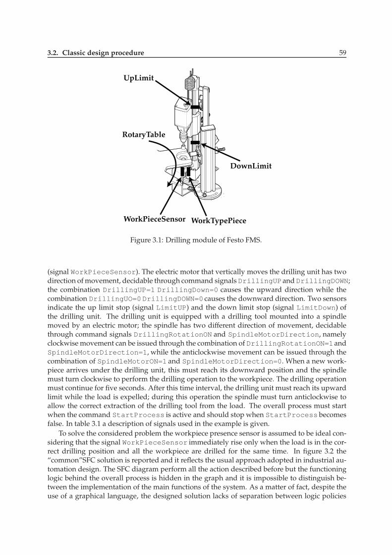
3.2. Classic design procedure 59
UpLimit
DownLimit
RotaryTable
WorkPieceSensor WorkTypePiece
Figure 3.1: Drilling module of Festo FMS.
(signal WorkPieceSensor). The electric motor that vertically moves the drilling unit has twodirection of movement, decidable through command signals DrillingUPand DrillingDOWN;the combination DrillingUP=1 DrillingDown=0 causes the upward direction while thecombination DrillingUO=0DrillingDOWN=0 causes the downward direction. Two sensorsindicate the up limit stop (signal LimitUP) and the down limit stop (signal LimitDown) ofthe drilling unit. The drilling unit is equipped with a drilling tool mounted into a spindlemoved by an electric motor; the spindle has two different direction of movement, decidablethrough command signals DrillingRotationON and SpindleMotorDirection, namelyclockwise movement can be issued through the combination of DrillingRotationON=1andSpindleMotorDirection=1, while the anticlockwise movement can be issued through thecombination of SpindleMotorON=1 and SpindleMotorDirection=0. When a new work-piece arrives under the drilling unit, this must reach its downward position and the spindlemust turn clockwise to perform the drilling operation to the workpiece. The drilling operationmust continue for five seconds. After this time interval, the drilling unit must reach its upwardlimit while the load is expelled; during this operation the spindle must turn anticlockwise toallow the correct extraction of the drilling tool from the load. The overall process must startwhen the command StartProcess is active and should stop when StartProcess becomesfalse. In table 3.1 a description of signals used in the example is given.
To solve the considered problem the workpiece presence sensor is assumed to be ideal con-sidering that the signal WorkPieceSensor immediately rise only when the load is in the cor-rect drilling position and all the workpiece are drilled for the same time. In figure 3.2 the“common”SFC solution is reported and it reflects the usual approach adopted in industrial au-tomation design. The SFC diagram perform all the action described before but the functioninglogic behind the overall process is hidden in the graph and it is impossible to distinguish be-tween the implementation of the main functions of the system. As a matter of fact, despite theuse of a graphical language, the designed solution lacks of separation between logic policies
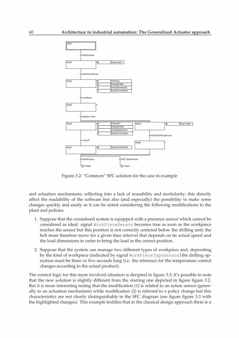
60 Architecture in industrial automation: The Generalized Actuator approach
Step1
StartProcess
Step2 N RotaryTable
WorkPieceSensor
Step3 S
R
S
S
LimitDown
Step4
Step4t>=T#5s.
Step5
LimitUP
Step7
Step6 N RotaryTable
NOT
Step8
StartProcess
Step2
NOT StartProcess
Step1
DrillingUp
DrillingDOWN
DrillingRotationOn
RotationClockWise
R
S
S
R
DrillingUP
DrillingDOWN
DrillingRotationOn
RotationClockWise
R RotationClockWise
WorkPieceSensor
Figure 3.2: “Common” SFC solution for the case in example
and actuation mechanisms, reflecting into a lack of reusability and modularity; this directlyaffect the readability of the software but also (and especially) the possibility to make somechanges quickly and easily as it can be noted considering the following modifications to theplant and policies.
1. Suppose that the considered system is equipped with a presence sensor which cannot beconsidered as ideal: signal WorkPieceSensor becomes true as soon as the workpiecereaches the sensor but this position is not correctly centered below the drilling unit; thebelt must therefore move for a given time interval that depends on its actual speed andthe load dimensions in order to bring the load in the correct position.
2. Suppose that the system can manage two different types of workpiece and, dependingby the kind of workpiece (indicated by signal WorkPieceTypeSensor) the drilling op-eration must be three or five seconds long (i.e. the reference for the temperature controlchanges according to the actual product).
The control logic for this more involved situation is decipted in figure 3.3; it’s possible to notethat the new solution is slightly different from the starting one depicted in figure figure 3.2.But it is more interesting noting that the modification (1) is related to an action sensor (gener-ally to an actuation mechanism) while modification (2) is referred to a policy change but thischaracteristics are not clearly distinguishable in the SFC diagram (see figure figure 3.3 withthe highlighted changes). This example testifies that in the classical design approach there is a
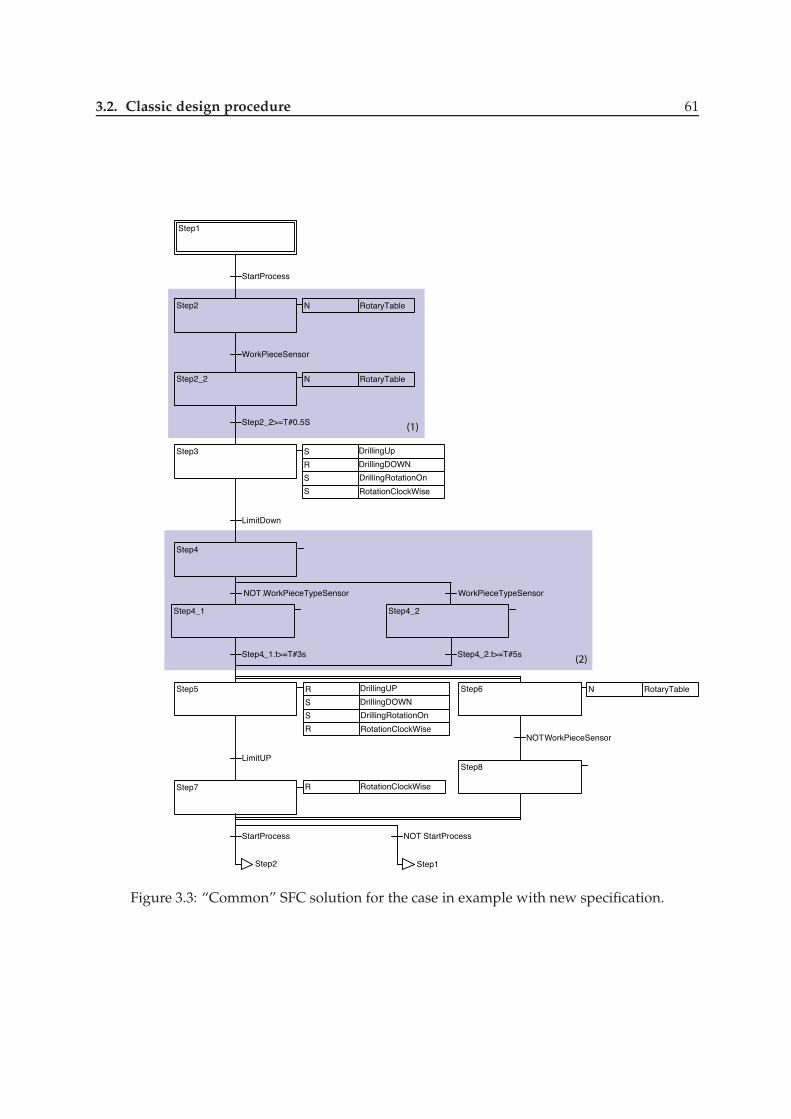
3.2. Classic design procedure 61
(2)
(1)
Step1
StartProcess
Step2 N RotaryTable
Step2_2>=T#0.5S
Step3 S
R
S
S
LimitDown
Step4
Step4_1.t>=T#3s.
Step5
LimitUP
Step7
Step6 N RotaryTable
NOT
Step8
StartProcess
Step2
NOT StartProcess
Step1
DrillingUp
DrillingDOWN
DrillingRotationOn
RotationClockWise
R
S
S
R
DrillingUP
DrillingDOWN
DrillingRotationOn
RotationClockWise
R RotationClockWise
WorkPieceSensor
WorkPieceSensor
Step2_2 N RotaryTable
. WorkPieceTypeSensor
Step4_1 Step4_2
Step4_2.t>=T#5s.
NOT WorkPieceTypeSensor
Figure 3.3: “Common” SFC solution for the case in example with new specification.

62 Architecture in industrial automation: The Generalized Actuator approach
Signal Meaning TypeStartProcess Operator command to start the process DigitalRotaryTable Command signal to move the rotary table Digital
WorkPieceSensor Workpiece presence sensor readings DigitalWorkPieceTypeSensor Workpiece type sensor readings Digital
DrillingDown Command signal to move the drilling unit down DigitalDrillingUp Command signal to move the drilling unit upt Digital
LimitUP Drilling upward limit signal DigitalLimitDOWN Drilling downward limit signal Digital
DrillingRotationON Command signal to move the spindle DigitalSpindleMotorDirection Command signal to motion direction for the spindle Digital
Table 3.1: List of signals used in the drilling example
Step1
StartProcess
Step2 N RotaryTable
WorkPieceSensor
Step3 S
R
S
S
LimitDown
Step4
Step4t>=T#5s.
Step5
LimitUP
Step7
Step6 N RotaryTable
NOT
Step8
StartProcess
Step2
NOT StartProcess
Step1
DrillingUp
DrillingDOWN
DrillingRotationOn
RotationClockWise
R
S
S
R
DrillingUP
DrillingDOWN
DrillingRotationOn
RotationClockWise
R RotationClockWise
WorkPieceSensor
NOT WorkPieceSensor AND Step2.t>=T#8S
Step3_F N FAULT1
ENDFAULT1
Step3_R
Step1
NOT LimitDown AND Step3.t>=T#10S
Step4_F N FAULT2
ENDFAULT2
Step4_R
Step1
NOT WorkPieceSensor AND Step2.t>=T#3S
Step8_F N FAULT1
ENDFAULT1
Step8_R
Step1
NOT LimitUP AND Step5.t>=T#10S
Step7_F N FAULT3
ENDFAULT3
Step7_R
Step1
Figure 3.4: “Common” SFC solution for the case in example with fault.
mixing between mechanisms and policies and testifies also how this mixing minimize both themodularity and the reusability of the control software. The lack of reusability can be explainedin this way: in the case in the drilling station of the example must be used in another systembut in a different mode, it is clear that the software designed shown in figure figure 3.2 or fig-ure 3.3 cannot be reused (typically) without some modifications. Generally, all the control logicare designed for each machine because the adaptation of parts of existing software is difficultin industrial automated systems.Another worthy remark concerning the solution of figures figure 3.2 and figure 3.3 is to note
that the diagnostic phase has been completely disregarded. Even diagnosis of anomalous situ-ations can be considered at two different levels: detection of mechanisms failures (e.g. sensoror actuator faults, components malfunctioning, etc.) and functional anomalies (e.g. forbiddencontrol sequences that occur due to external influences). If we consider possible faults on sen-sors or actuators on case of the drill unit we can define a control logic as in figure 3.4, while if weconsider the faults on drill unit with the modification (1) and (2) we can define a control logicas in figure 3.5. If we compare the starting solution (see fig. 3.2) and the solution with faults

3.3. Generalized Actuator approach 63
(2)
(1)
Step1
StartProcess
Step2 N RotaryTable
Step2_2>=T#0.5S
Step3 S
R
S
S
LimitDown
Step4
Step4_1.t>=T#3s.
Step5
LimitUP
Step7
Step6 N RotaryTable
NOT
Step8
StartProcess
Step2
NOT StartProcess
Step1
DrillingUp
DrillingDOWN
DrillingRotationOn
RotationClockWise
R
S
S
R
DrillingUP
DrillingDOWN
DrillingRotationOn
RotationClockWise
R RotationClockWise
WorkPieceSensor
NOT WorkPieceSensor AND Step2.t>=T#8S
Step3_F N FAULT1
ENDFAULT1
Step3_R
Step1
NOT LimitDown AND Step3.t>=T#10S
Step4_F N FAULT2
ENDFAULT2
Step4_R
Step1
NOT WorkPieceSensor AND Step2.t>=T#3S
Step8_F N FAULT1
ENDFAULT1
Step8_R
Step1
NOT LimitUP AND Step5.t>=T#10S
Step7_F N FAULT3
ENDFAULT3
Step7_R
Step1
WorkPieceSensor
Step2_2 N RotaryTable
. WorkPieceTypeSensor
Step4_1 Step4_2
Step4_2.t>=T#5s.
NOT WorkPieceTypeSensor
Figure 3.5: “Common” SFC solution for the case in example with new specification and fault.
(see fig. 3.2) it is important to note how add some simple specification the control logic has anexplosion of complexity. Another note is regarding that a control logic as the one presentedin figure figure 3.2 and figure 3.3 prevents from obtaining a separation between mechanismsdiagnostics and policies diagnostics; then also for diagnostic software are preferable character-istics of modularity and reusability especially when it is required the system to be tolerant tofaults having to distinguish between mechanisms reliability (e.g. considering redundancy) andpolicies reconfigurability (e.g. switching between different control logic).
3.3 Generalized Actuator approach
The novel approach proposed in this thesis starts from the idea of considering logic control asa recipe mainly composed by two ingredients: (i) a set of basic actions, (ii) one or more de-sired sequences to coordinate actions execution. The first ingredient represents mechanisms offunctionality implementation, while the second represents the control policy. As enlightenedpreviously the needs for reusable, modular control software require the two to be completelyindependent. First of all, all the action/mechanisms are defined, using the GA entity; after-wards the overall control policy is considered.The first step for mechanism definition is to identify basic actions that cannot be reasonablyfurthermore decomposed. For the considered system the basic actions to perform are (1) movethe workpiece in drilling position, indicated as Positioning; (2) expel the drilled workpiece,

64 Architecture in industrial automation: The Generalized Actuator approach
indicated as Expulsion; (3) move the drill unit upward, indicated as DrillGoUp; (4) movethe ram downward, indicated as DrillGoDown; (5) control the spindle rotation, indicated asSpindleControl.Each basic action is then associated with a set of actuators and sensors that physically performthe action. As depicted in figure 3.6, action Positioning and Expulsion both involve sensorWorkPieceSensor and actuator RotaryTable. Actions DrillGoUp and DrillGoDown in-volve sensorsLimitUP and LimitDOWN, respectively, and actuators DrillUP and DrillDOWN,both of them. Finally action SpindleControl involves actuators DrillingRotationONand SpindleMotorDirection. At this point, the proposed subsequent step is the effective
Actions Sensors Actuators
Positioning
DrillGoUP
DrillGoDOWN
Expulsion
SpindleControl
WorkPieceSensor, WorkPieceTypeSensor
LimitUP
LimitDown
DrillUP, DrillDOWN
DrillingRotationON, SpindleMotorDirection
RotaryTable
RotaryTable
DrillUP, DrillDOWN
WorkPieceSensor
Actions Sensors Actuators
Positioning
DrillGoUP
DrillGoDOWN
Expulsion
SpindleControl
WorkPieceSensor, WorkPieceTypeSensor
LimitUP
LimitDown
DrillUP, DrillDOWN
DrillingRotationON, SpindleMotorDirection
RotaryTable
RotaryTable
DrillUP, DrillDOWN
WorkPieceSensor
Actions Sensors Actuators
Positioning
DrillGoUP
DrillGoDOWN
Expulsion
SpindleControl
WorkPieceSensor, WorkPieceTypeSensor
LimitUP
LimitDown
DrillUP, DrillDOWN
DrillingRotationON, SpindleMotorDirection
RotaryTable
RotaryTable
DrillUP, DrillDOWN
WorkPieceSensor
Actions Sensors Actuators
Positioning
DrillGoUP
DrillGoDOWN
Expulsion
SpindleControl
WorkPieceSensor, WorkPieceTypeSensor
LimitUP
LimitDown
DrillUP, DrillDOWN
DrillingRotationON, SpindleMotorDirection
RotaryTable
RotaryTable
DrillUP, DrillDOWN
WorkPieceSensor
Figure 3.6: Actions, sensors and actuators of the systems.
definition of GAs following this basic concept (which is a sort of definition of a GA): every GAis a “virtual”actuator with the following characteristics:
- it is in charge of the execution of a small subset of the basic actions identified in previous

3.4. Generalized actuator definition and design procedure formalization 65
steps (hence it handles actuators and sensor associated to them);
- it is always “alive” during the operations of the automation plant, even if no specific actionis required to it.
In order to give effective “guide-lines”for this phase, the following rules are introduced:
- the union of the actuators associated with the set of GAs must be equal to the whole ac-tuators set of the system (for what concern the sensors usually the same condition shouldbe satisfied but it is not mandatory);
- pursuing a non interference idea, sets of sensors and actuators belonging to different GAsmust be disjointed.
In the considered example, the situation depicted in lower part of figure 3.6 is obtained. Look-ing for common equipment used in different actions, leads to group them in three GAs re-spectively devoted to the drilling workpiece, move the drill unit and control spindle rotationcontrol.From the considered example, it is immediate to note that there exist two different kinds ofactions and, consequently, of GAs; there are actions which structurally terminate after a fi-nite time (e.g. action Positioning implies moving the belt until the workpiece reaches thedrilling position), while there are others which, in principle, could continue for an infinite timeand whose termination has to be decided “externally”(e.g. action SpindleControl).The GAs associated to the first kind of actions are denominated Do-Done GA. They are charac-terized by a input signal Do used to command the starting of an action, an input signal DoWhatto specify what kind of action has to be performed (if more than one is available) and an outputsignal Done to signal when the action has terminated successfully.Differently, the GAs associated to the second kind of actions are denominated Start-Stop GA.Their characteristic I/O signals are the input Start to command the beginning of an action,defined by the input StartWhat, and the input command Stop to stop the action.For the presented example, the following GAs can be defined:
• WorkPieceMotion, a Do-Done GA that is devoted to workpiece positioning;
• DrillMotion, a Do-Done GA that is aimed at moving the drill unit;
• Spindle, a Start-Stop GA that is aimed at controlling the spindle rotation of drilling.
These three GAs are described and realized using the Function Block (FB) formalism definedin IEC61131-3 (see appendix B to see the code). It is worth noting that the FB are not used bychance, in fact they represent Program Organization Units (POUs) which have to be alwaysactive during overall control execution.
3.4 Generalized actuator definition and design procedure formaliza-tion
We are now ready to define the structure of a GA specializing its input/output interface and itsbasic dynamics by means of a state diagram; after that, generalizing the procedure proposed insection 3.3 to solve the benchmark example, we furnish some guidelines to design the controllogic using the GA approach.

66 Architecture in industrial automation: The Generalized Actuator approach
In Figure 3.7 the interface section of both Do-Done GA (Figure 3.7(a)) and Start-Stop GA(Figure 3.7(b)) are depicted; in both cases the interface can be mainly divided in two sections inthe following described.
1. Interface to policy: this section represents the input/output section between the GA andthe supervision policy. It can be further decomposed in two subsections separating thestandard communications between the GA and the policy and all the case dependentcommunications.
Standard interface: embeds all command inputs for the GA and the outputs that com-municate the actual state of the GA and the task that it is accomplishing. More indetails the Do-Done GA will receive as command the Do signal to start operationsand the DoWhat signal to specify the desired action, while the Start-Stop GA will becommanded through inputs Start to start operations and Stop to conclude oper-ations, and through signal StartWhat to define the required action. In both casesinput signals Alarm, AlarmType can be used to communicate to the GA the oc-currence of an external anomalous situation. The outputs of this section are, for theDo-Done GA, the Done signal by which the GA communicate that the task has beenperformed and the DoneWhat signal by which the terminated task is specified; theStart-Stop GA outputs are the signal DoingWhat representing the task that the GAis performing. In both kind of GAs, a State signal communicate the actual state inwhich the GA is evolving.
Communications: represents all the non standard communications between the policyand the GA, as the results of sensor readings filtering (e.g. the WorkPieceTypeSensorsignals in WorkPieceMotor GA, that distinguish between two different kind ofworpiece filtering the sensor readings WorkPieceTypeSensor.
2. Low level interface: this section contain all the interfaces with the low level world; eventhis section can be further decomposed in two sub sections considering the constant pa-rameters used by the GA separated from the physical interconnection with the plant.
Constant parameters: contains all the inputs by which it is possible to give a constantvalue to characteristic parameters of the GA (e.g. in WorkPieceMotionGA the in-put PositioningDelayTime by which define the time interval between the acti-vating instant for sensorWorkPieceSensorand the instant in which the workpiecereaches the drilliing position.
Plant I/O link: is the real interface with the plant and contains as inputs all the links tosensors and as outputs the links to actuators. In this way the physical connectionbetween the GA and the plant is completely hidden to the high level control policy.
The GA should then be designed considering as Reference Model the event driven evolution infigure 3.7(c). In the depicted automaton it is possible to distinguish the states in the followingdescribed.
Init: this state is the initial one and becomes active as soon as the GA is activated (usuallyat the beginning of operations). It represents the state in which initialization actions areperformed; the GA moves out from this state when a signal EndInit communicates thatthe initialization operations are concluded forcing the GA to move in Ready state.
Ready: in this state the GA is ready to perform the desired operation and is waiting for the Door Start command to move to Busy state.

3.4. Generalized actuator definition and design procedure formalization 67
DoDoWhat
DoneDoneWhat
State
Interface to policy
Standard Interface
Communication
Low level interface
Constant Parameters
Plant I/O link
(a) Do-Done GA interface.
StartStop
DoingWhatState
Interface to policy
Standard Interface
Communication
Low level interface
Constant Parameters
Plant I/O link
StartWhat
(b) Start-Stop GA interface.
Init Ready Busy
Fault
Start
Process EndInit
Do/Start
Done/Stop
Fault Fault
Fault
EndFault
(c) GA evolution model.
Figure 3.7: Interfaces of GAs.
Busy: after the command issued by the policy the GA starts performing its required task com-municating with the high level policy information on the accomplishment of the function(e.g. information on the quality of the operations). The GA remains into this state untilthe task is finished and the signal Done is raised (Do–Done GA) or until the Stop signal(Start–Stop GA) is issued by the policy. In these cases the GA moves back to state Ready.
Fault: from any state a signal Fault (used to communicate some anomalies) can force theGA to move into a Fault state in which some counteractions are taken. Note that theFault signal can be both due to external commands (e.g. an alarm issued by an externaloperator), to internal diagnostics or to wrong logic operations. When the alarm situationis concluded (signal EndFault) the GA returns in the Init state to be reinitialized.
It is important to stress that each of the states just described represent a set of states; in thissense the automaton in figure 3.7(c) plays the role of a logic design pattern similarly to GEMMAdiagram (see [65]).
To conclude this Section we briefly summarize the design procedure based on GAs andintroduced in section before:
1. Identify basic actions of the process;
2. Define Do-Done actions;
3. Define Start-Stop actions;
4. Identify the GAs by grouping actions with overlapping sets of sensors or actuators;
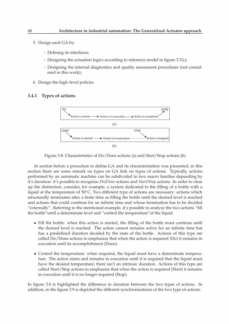
68 Architecture in industrial automation: The Generalized Actuator approach
5. Design each GA by:
- Defining its interfaces;
- Designing the actuation logics according to reference model in figure 3.7(c);
- Designing the internal diagnostics and quality assessment procedures (not consid-ered in this work);
6. Design the high–level policies
3.4.1 Types of actions
DO DONE
Action is started Action is in execution Action is completed
(a)
START STOP
Action is started Action is in execution Action is stopped
(b)
Figure 3.8: Characteristics of Do/Done actions (a) and Start/Stop actions (b)
In section before a procedure to define GA and its characterization was presented, in thissection there are some remark on types on GA link on types of actions. Typically, actionsperformed by an automatic machine can be subdivided in two macro families depending byit’s duration: it’s possible to recognize Do/Done actions and Start/Stop actions. In order to clearup the distinction, consider, for example, a system dedicated to the filling of a bottle with aliquid at the temperature of 50◦C. Two different type of actions are necessary: actions whichstructurally terminates after a finite time as filling the bottle until the desired level is reachedand actions that could continue for an infinite time and whose termination has to be decided“externally”. Referring to the mentioned example, it’s possible to analyze the two actions “fillthe bottle”until a determinate level and “control the temperature”of the liquid.
• Fill the bottle: when this action is started, the filling of the bottle must continue untilthe desired level is reached. The action cannot remains active for an infinite time buthas a predefined duration decided by the state of the bottle. Actions of this type arecalled Do/Done actions to emphasize that when the action is required (Do) it remains inexecution until its accomplishment (Done).
• Control the temperature: when required, the liquid must have a determinate tempera-ture. The action starts and remains in execution until it is required that the liquid musthave the desired temperature; there isn’t an intrinsic duration. Actions of this type arecalled Start/Stop actions to emphasize that when the action is required (Start) it remainsin execution until it is no longer required (Stop).
In figure 3.8 is highlighted the difference in duration between the two types of actions. Inaddition, in the figure 3.9 is depicted the different synchronizations of the two type of actions.

3.5. GA in rapid prototyping 69
DO
DONE
Action Performed
(a) Do-Done GA actions.
START
STOP
Action in execution
(b) Start-Stop GA actions.
Figure 3.9: Characteristic of GAs action.
3.5 GA in rapid prototyping
Time-to-market is a crucial issue in developing any industrial product and, consequently, therequest of reducing development time in realizing automated industrial plants is getting moreand more stringent. Toward this purpose, many tools have been developed to speed-up thetesting phase of logic control in the typical development life-cycle. These items are basicallysimulation tools and rapid prototyping tools. The latter have been recently introduced to speedup the testing of the final SW or HW/SW implementing the control algorithms, following thesoftware-in-the-loop or the hardware-in-the-loop approaches, respectively (see, beside others,[16], [23] and [63]). In particular, the integration between simulation frameworks and rapidprototyping platforms based on automatic code generation tools has relevantly increased thespeed and reliability of the translation from abstract definition of control algorithms to the cor-responding implementing software. In this section we’ll see how GAs help the designer inrapid prototyping of control logic in complex industrial automated systems.With the term rapid prototyping we refer to a set of methods and tools to solve and verify controlproblems fast and efficiently resulting in a functioning controller prototype; such techniquesinclude theoretical methods of control engineering from designing a system model and sys-tem analysis to the design of a control strategy, test and optimization of the control strategyin a simulation environment, automatic code generation for a real-time system operating a teststand and verification and optimization of the controller with the target object on the test stand.When dealing with complex systems, an efficient strategy is to decompose (usually followingfunctional reasoning) the system and verifying each of these parts, leaving the testing of theintegration of the whole system as a final step. The challenge in this task is to choose the rightway to decompose the system in order to obtain reasonably simple sub-systems while guaran-teeing a certain degree of modularity. To this aim, GA can can play a key role; the idea is tofollow the same reasoning used to design the control logic to verify its correctness, dividing theactuation mechanisms from the desired policies while leaning on the concepts used to defineGAs in order to have a suitable decomposition of the system. This strategy helps in defininga set of simple and verified actuation bricks pursuing the idea of modular, reusable and easilymaintainable control software: changing actuation mechanisms or changing coordination pol-icy can be treated separately.In order to better enlighten the advantages of this technique, we apply the GA concept to a big-ger part, than the part presented in section 3.2 ,of FESTO manufacturing system. In figure 3.10is presented the proccessing station of the system, The station allows three parallel operationsthanks to a six position rotary table and three working modules: testing module, drilling mod-ule and pushing out device. For an exhaustive description of the processing station the readeris referred to B; in the following the desired sequence of operation for this station is described.

70 Architecture in industrial automation: The Generalized Actuator approach
When a workpiece is loaded from the distribution station to the rotary table (signal AVAI-BLELOADFORWORKINGSTATION becomes active), the table must rotate to move the workpieceto the first working unit. To this aim the table is actuated through the command signal ROTA-RYTABLEMOTOR and is equipped with a sensor that indicates when the rotary table is aligned(signal ALIGNMENTROTARYTABLEWITHPOSITIONINGS).
WORKPIECE FROM
PREVIOUS STATION
WORKPIECE
TO NEXT
STATION
TESTING
MODULE
DRILLING
MODULE
PUSHING-OUT
MODULE
CLAMPING
DEVICE
Figure 3.10: Processing station.
When a workpiece is detected in the rotary table, this last makes a 60◦ rotation (correspond-ing to the shift of the six working positions) to move the workpiece to the first module of theprocessing station: the testing module. This module must control if the actual workpiece (itspresence is communicated by signal AVAIBLELOADINCONTROLPOSITIONING) has a correctorientation or is upside-down. To do this, the module is equipped by a cylinder actuatedthrough signal TOLOWERCYLINDERTOINSPECTLOAD, which moves downward and checkswhether the workpiece is inserted with the opening facing upwards. If the workpiece is in theright position (signal INCONTROLLOADINWRONGPOSITIONTOBEDRILLED is active) it can bedrilled, otherwise it must be expelled from the system.
After this testing module, the workpiece is moved to the drilling module by a table rotation;

3.5. GA in rapid prototyping 71
when the actual piece is under the drilling machine (signal AVAILABLELOADINDRILLINGPOSI-TIONING is active), the clamping device clamps the workpiece (actuation signal BLOCKINGCY-LINDERFORWARDINDRILLINGPOSITIONING) and the drilling operation can start. The drillingmachine is activated (actuation signal DRILLINGUNITACTIVE) with a clockwise rotation (ac-tuation signal DRILLINGUNITCLOCKWISE) and is moved downward (actuation signal TOLO-WERDRILLINGUNIT) until it reaches its lower limit (signal DRILLINGUNITDOWN). When thisposition is reached, the driller machine should continue its operation for 2 seconds and, afterthis time period, it is moved upward (actuation signal TOLIFTDRILLINGUNIT) with a counter-clockwise rotation (actuation signal DRILLINGUNITUNCLOCKWISE) until it reaches its higherlimit position (signal DRILLINGUNITUP). At this point the drilling operation is concluded andthe drilling machine can be stopped deactivating signal DRILLINGUNITACTIVE, while retract-ing the clamping device (deactivation of signal BLOCKINGCYLINDERFORWARDINDRILLING-POSITIONING).
With one more 60◦ rotation of the rotating table the workpiece arrives to the last module: thepushing-out module. When a workpiece is within this module (this situation is not recordedby any sensor), a mechanical link actuated by signal EXPELLINGLEVERACTIVE expels it to theassembly station. If the piece was recognized to be upside-down, an alarm light (actuated bysignal LIGHTUPSIDEDOWNLOADINEXPELLING) communicates this situation and the systemis stopped waiting for a manual removal of the piece. In table B.3, in appendix B, signals usedin the testbed are listed as well as their activation meaning.
The first step to define Ga as explained in section 3.3 is to identify basic actions required tothe plant; these can be described as follows.
1. RotaryTableActive: move the rotary table.
2. ToLowerCylinderToInspectLoadActive: move downward the testing device.
3. ToLiftCylinderToInspectLoadActive: move upward the testing device.
4. BlockingCylinderForwardInDrillingPositioningActive: clamp the workpiece for drilling.
5. BlockingCylinderBehindInDrillingPositioningActive: disable the clamp to unlock the work-piece after drilling.
6. ToLowerDrillingUnitActive: move downward the drilling device.
7. ToLiftDrillingUnitActive: move upward the drillling device.
8. DrillingUnitClockWiseActive: rotate the drilling device clockwise.
9. DrillingUnitUnClockWiseActive: rotate the drilling device counterclockwise.
10. ExpellingLeverForwardActive: move the arm that expels the workpiece.
11. ExpellingLeverBehindActive: release the arm that expels the workpiece.
It is important to note that, when defining basic actions, we introduce some redundancy. Forexample for clamping device, we only command its closure (activation of signal BLOCKINGCY-LINDERFORWARDINDRILLINGPOSITIONING), while the release action is implicit in the deacti-vation of command signal (in this case a spring mechanism allow the release action); however,we list also the clamp unlock action. This is mainly due to the effort of completely decouple

72 Architecture in industrial automation: The Generalized Actuator approach
Act. Sensors Actuators
1 ALIGNEMENTROTARYTABLEWITHPOSITIONING ROTARYTABLEMOTOR
2 INCONTROLLOADINWRONGPOSITIONTOBEDRILLED TOLOWERCYLINDERTOINSPECTLOAD
AVAILABLELOADINCONTROLPOSITIONING
3 TOLOWERCYLINDERTOINSPECTLOAD
4 AVAILABLELOADINDRILLINGPOSITIONING BLOCKINGCYLINDERFORWARDINDRILLINGPOSITIONING
5 BLOCKINGCYLINDERFORWARDINDRILLINGPOSITIONING
6 DRILLINGUNITDOWN TOLOWERDRILLINGUNIT
DRILLINGUNITUP TOLIFTDRILLINGUNITUP
7 DRILLINGUNITDOWN TOLOWERDRILLINGUNIT
DRILLINGUNITUP TOLIFTDRILLINGUNITUP
8 DRILLINGUNITCLOCKWISE
DRILLINGUNITACTIVE
9 DRILLINGUNITUNCLOCKWISE
DRILLINGUNITACTIVE
10 UPSIDEDOWNLOADREMOVEDINEXPELLING EXPELLINGLEVERACTIVE
LIGHTUPSIDEDOWNLOADINEXPELLING
11 EXPELLINGLEVERACTIVE
Table 3.2: List of sensors and actuators associated to actions.
policy from mechanisms: the policy is interested in issuing the unlock command, while com-pletely disregarding the physical mechanism that allow the action. Role of the GAs devoted toaccomplish such actions will be to map the actions into correct signal sequences.
Once we have defined basic actions, the second step is to associate to each action the set ofsensors and actuators that are involved (see Table 3.2.
At this point, following the procedure presented in 3.3, it is possible to define the followingGAs1:
• RotaryTable (DD): implements action 1;
• ControlUnit (DD): implements actions 2-3;
• BlockingCylinderInWorkingStation (DD): implements actions 4-5;
• DrillingUnit (DD): implements actions 6-7;
• DrillControl (SS): implements actions 8-9;
• ExpellingUnit (DD): implements actions 10-11;
Logic control of the drilling module deserves a further explanation; three GAs are devoted tosuch task (namely BlockingCylinderInWorkingStation, DrillingUnit and DrillingControl).In fact, the drilling operation issued by the policy can be further decomposed in sub-operations:(i) lock workpiece, (ii) drill the workpiece, (iii) extract the drilling unit and (iv) unlock the work-piece. Moreover drill the workpiece action can be decomposed in (a) activate the drilling unitwith a clockwise rotation, (b) move downward the drilling unit until its lower limit is reachedand (c) wait for 2 seconds in this position while the extract the drilling unit action means (a)lifting the drilling unit while (b) rotating counterclockwise. Such sequences of actions reflect in
1Label SS stands for Start-Stop GA, while label DD stands for DoDone GA.
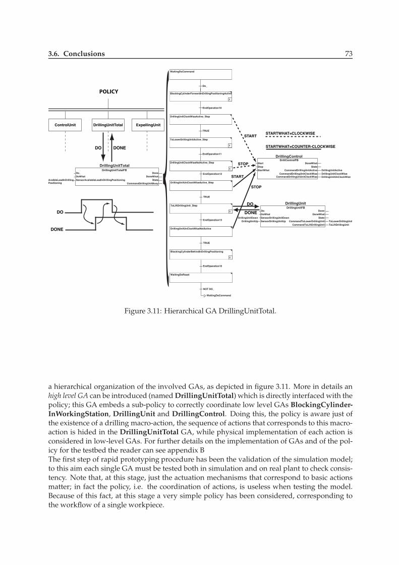
3.6. Conclusions 73
X
WaitingDoCommand
Do_
BlockingCylinderForwardInDrillingPositioningActive
X
EndOperation10
DrillingUnitClockWiseActive_Step
ToLowerDrillingUnitActive_Step
X
EndOperation11
DrillingUnitClockWiseNotActive_Step
EndOperation12
DrillingUnitUnClockWiseActive_Step
ToLiftDrillingUnit_Step
X
EndOperation13
DrillingUnitUnClockWiseNotActive
BlockingCylinderBehindInDrillingPositioning
X
EndOperation16
WaitingDoReset
NOT DO_
WaitingDoCommand
POLICY
DrillingUnitTotal ExpellingUnitControlUnit
DrillingUnitTotalFB
DrillingUnitTotal
Do_
DoWhat
SensorAvailableLoadInDrillingPositioning
Done
DoneWhat
State
CommandDrillingUnitBusy
AvaibleLoadInDrilling
Positioning
DO DONE
TRUE
TRUE
TRUE
DO
DONE
DrillControlFBStart
Stop
StartWhat
DoneWhat
State
CommandDrillingUnitActive
CommandDrillingUnitClockWise
DrillingUnitActive
DrillingUnitClockWise
DrillingControl
CommandDrillingUnUnitClockWise DrillingUnitUnClockWise
START
STOP
STOP
START
STARTWHAT=CLOCKWISE
STARTWHAT=COUNTER-CLOCKWISE
DrillingUnitFB
DrillingUnit
Do_
DoWhat
SensorDrillingUnitDown
SensorDrillingUnitUp
Done
DoneWhat
State
CommandToLowerDrillingUnit
CommandToLiftDrillingUnit
ToLowerDrillingUnit
ToLiftDrillingUnit
DrillingUnitDown
DrillingUnitUp
DO
DONE
Figure 3.11: Hierarchical GA DrillingUnitTotal.
a hierarchical organization of the involved GAs, as depicted in figure 3.11. More in details anhigh level GA can be introduced (named DrillingUnitTotal) which is directly interfaced with thepolicy; this GA embeds a sub-policy to correctly coordinate low level GAs BlockingCylinder-InWorkingStation, DrillingUnit and DrillingControl. Doing this, the policy is aware just ofthe existence of a drilling macro-action, the sequence of actions that corresponds to this macro-action is hided in the DrillingUnitTotal GA, while physical implementation of each action isconsidered in low-level GAs. For further details on the implementation of GAs and of the pol-icy for the testbed the reader can see appendix BThe first step of rapid prototyping procedure has been the validation of the simulation model;to this aim each single GA must be tested both in simulation and on real plant to check consis-tency. Note that, at this stage, just the actuation mechanisms that correspond to basic actionsmatter; in fact the policy, i.e. the coordination of actions, is useless when testing the model.Because of this fact, at this stage a very simple policy has been considered, corresponding tothe workflow of a single workpiece.

74 Architecture in industrial automation: The Generalized Actuator approach
MASTER POLICY
Slave 1 Slave 2 Slave n
Init Main Test
GA 1 GA 2 GA 3 GA 4
Do/Done Start/Stop Do/Done Do/Done
GA 1
GA 2
GA 3
GA 4
GA 1
GA 2 GA 3 GA 4
Figure 3.12: An example of policy manager with GA approach.
3.6 Conclusions
In chapter 2 and in section 3.1 it was presented different approach to design control logic in in-dustrial automated systems and their limitation. In this chapter it was present an architecturefor industrial automated systems based on the novel concept of the Generalized Actuator.The design procedure to realize automation functions exploiting a clear and structural sepa-ration between policies and actions has been introduced To this aim a novel entity denoted asGeneralized Actuator (GA) is defined in order to (i) encapsulate actuation mechanisms separatingthem from high level control policies in order to hierarchically manage the plant, (ii) supporthardware virtualization, component interoperability and reusability and (iii) make easier thedesign of diagnostics, reconfiguration and quality check functionalities exploiting a distributedand hierarchical approach. Usually in automated systems the machine has different operationmode, like initialization mode, test mode, etc. These different operation modes have different“sub policies”which interact with the same actuators and sensors but with a different coordina-tion, like it’s possible to see in figure 3.12. From this point of view is clear as GA approach helpthe designer in the design of the entire control logic, in fact the different policies use the sameGA but only in a different order or coordination, but actuation mechanism defined by GA arethe same, we can image a GA like a musician and the policy like the conductor, the musician isalways the same but the conductor “drive”the musician in a different way.Actually the emphases has been put on the improvements obtained in terms of modularity andreusability, but it is also important to stress that the proposed procedure, that reflects into a hi-erarchical architecture, is the starting step towards a hierarchical diagnostics systems, in whichmechanisms fault diagnosis is separated from policy safety verification, and especially towardsa hierarchical reconfiguration system in which fault counteractions can be taken separately atmechanisms level and/or at policy level.In chapter 2 is shown the standard ISA S88 which define a hierarchical approach with the con-cept of recipe. The main difference in GA approach is the policy is completing separate fromthe actuation mechanism. In S88 the equipment phase, a sort of low level, implements a part oflogic to know if this operation is safe for the process. In this way the low level have to know apart of policy, and this part of policy is dependent from application this means the equipmentphase can not be reusable in a different process because the part of logic inside change from ap-

3.6. Conclusions 75
plication to another. Another point is, with the S88 the policy is distributed on all the systemsand this cause a difficult to test its correctness.

76 Architecture in industrial automation: The Generalized Actuator approach

Chapter 4The Generalized Device concept
This chapter introduces and analyzes a novel entity called Generalized
Device (GD) for logic control and diagnosis of field devices in industrialautomation. The emphasis has been particularly put on the diagnosticfunctionalities embedded within the GD entity. In addition, it has beenshown that, following an inheritance principle, starting from the basicGD, other typologies can be easily derived. The case study enlightenshow to implement GDs for the control of field devices typically used inautomated manufacturing systems.
4.1 Actuation mechanism
In chapter 3 it was presented the novel concept of the Generalized Actuator, and it was ex-plained as GA can help the designer to develop the control logic in a modular way. One lim-itation of GA approach is that that GA has a standard interface but a specific GA componentcould be reused only if the plant part it handles is reused. In this chapter we’ll see how itis possible to define a new layer in architecture independent from hardware of a industrialautomated systems, this new entity is defined Generalized Device (GD). Analyzing the typicalsensorial/actuation equipment in a industrial automated systems it’s possible to find differentkind of actuators and sensors coming from different fields, so to define an entity independentfrom hardware implementation we have to answer to this questions: “Do different field devicesreally need different control logic?”The term actuator is used for the device which transforms a signal (usually an electrical signal)into some more powerful action which then results in the control of the process, it is possibleto characterized the actuator in this fields:
• compressed air (pneumatics);
• hydraulics;
• electric motors.
77

78 The Generalized Device concept
A sensor is a device that measures a physical quantity and converts it into a signal whichcan be read by an observer or by an instrument. Sensors are designed and built to address avery different kind of task and can be so different, some sensors are very simple, like positionsensors, and there are sensors with a complicate structure, like vision sensor. Usually on aindustrial automated system we can find a numerous simple sensors and perhaps a singlevision implementation at best. In this section we’ll see the main characteristic of sensors, a firstclassification can be made respect of information generates by the sensor: (i) a discrete binary(on/off) situation, (ii) a continuous value.An example of discrete sensor it is a sensor used to determinate if a box had been propelledinto a limit switch mounted on a movable stop. The information generates from the sensor is ifthere is the box or it is not. It cannot tell if the box is getting close, or what speed or force thebox has when it hits. A continuous sensor can tell you some value that is likely to change quitequickly, for example a pressure sensor can measures the pressure of a gas or a liquid.A discrete sensor’s output is most likely digital, actuating a switch that completes a circuit ordisconnects it. Continuous sensor’s output can be either digital or analog. It depends on thetechnology and circuitry being used. Many times it is an analog value that is converted to adigital signal. An example would be the capacitance sensor used for left turn lanes at trafficlights. Many times a sensor wire that connects with the sensor controller is embedded into thepavement. A car with its significant metal mass changes the capacitance field, and the sensorcircuit takes the analog signal and determines the presence of a car, or not presence of the car.Then it tells the traffic light processor to take the option of giving a green left turn arrow ornot. This sensor has some threshold value for a car, and will often not reach this threshold fora smaller motor cycle. And one will never trigger the sensor with a bicycle. In the traffic lightexample, the sensor has its own dedicated circuitry or processor, so the traffic light controlcould be a simple set of relays, if it is an older model. One of the issues to investigate forone’s automation machine is where the analog signal gets processed. And even if the maincontroller is capable of performing such processing, will it be a burden and drag down theoverall machine performance. Sensors with built in processors have become quite popular forthis reason, as well as having a system that best matches the sensor to the processor. Properimplementation is easier. If a sensor has analog output, it will most likely need to be convertedto digital for the controller to process the information. Almost all controllers work on digitalsignals internally for the decision process. Some controllers have built-in analog inputs wherethe signal is converted internally, but smaller and less expensive controllers often do not havethis capability and need external conversion.Another sensor type distinction is that of how the sensor determines its value. Some sensorshave a direct physical contact other sensors determine the measurement from a distance. In thissense we can divide sensors in (i) contact and (ii) noncontact. Contact sensors have two majorconcerns, The first is that contact means that there is usually something physically moving,and that moving closes a switch. The second concern is that by contact sensing, the pressure ordrag on the item being sensed may change the process. If one is winding a thin film of plastic,and a contact sensor can occasionally poke a hole in the plastic, the information of the sensorwill not correctly. In general, contact sensors can be significantly cheaper than the noncontactequivalent. Some noncontact sensors also require significant knowledge of how to implementand adjust them, while a contact sensor’s mode of operation is usually obvious.
Pressure sensor : pneumatic line checking device. It is important to know that the compressedair is on and up to system requirements before assuming that air cylinders will functionsatisfactorily.
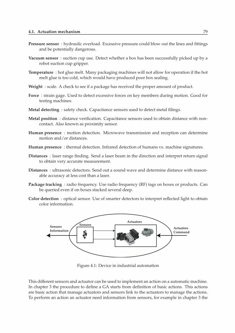
4.1. Actuation mechanism 79
Pressure sensor : hydraulic overload. Excessive pressure could blow out the lines and fittingsand be potentially dangerous.
Vacuum sensor : suction cup use. Detect whether a box has been successfully picked up by arobot suction cup gripper.
Temperature : hot glue melt. Many packaging machines will not allow for operation if the hotmelt glue is too cold, which would have produced poor box sealing.
Weight : scale. A check to see if a package has received the proper amount of product.
Force : strain gage. Used to detect excessive forces on key members during motion. Good fortesting machines.
Metal detecting : safety check. Capacitance sensors used to detect metal filings.
Metal position : distance verification. Capacitance sensors used to obtain distance with non-contact. Also known as proximity sensor.
Human presence : motion detection. Microwave transmission and reception can determinemotion and/or distances.
Human presence : thermal detection. Infrared detection of humans vs. machine signatures.
Distances : laser range finding. Send a laser beam in the direction and interpret return signalto obtain very accurate measurement.
Distances : ultrasonic detectors. Send out a sound wave and determine distance with reason-able accuracy at less cost than a laser.
Package tracking : radio frequency. Use radio frequency (RF) tags on boxes or products. Canbe queried even if on boxes stacked several deep.
Color detection : optical sensor. Use of smarter detectors to interpret reflected light to obtaincolor information.
SensorsActuators
Sensors Information
ActuatorsCommand
Figure 4.1: Device in industrial automation
This different sensors and actuator can be used to implement an action on a automatic machine.In chapter 3 the procedure to define a GA starts from definition of basic actions. This actionsare basic action that manage actuators and sensors link to the actuators to manage the actions.To perform an action an actuator need information from sensors, for example in chapter 3 the

80 The Generalized Device concept
operation of movement of drill unit up and down need information of two position sensors.We can define a device (see fig. 4.1) like a set of actuator and of sensors need to actuator toperform an action. From control logic point of view it is not important to know if the actuatoris electric or pneumatic or if the sensor is an inductor sensor or of other kind. The idea of theGeneralized Device is based on the concept that different device that perform the same actiondo not need different control logic, but the control logic will be dependent only by the numberof control actions and the number of sensors. This idea will be explained in the next section.
4.2 Devices classification
Taking inspiration from the pneumatic world, it’s possible to define the different kind of actu-ation mechanisms that composes a industrial automated system. Generally, plant is composedof pre-actuators, actuators and sensors. The pre-actuators transform the controller commandsinto power that is transformed by the actuators into actions performed by the effectors. Sen-sors are used to inform the controller about the effectors state. Pre-actuators can be classified
P1 A1
A2 P2
Piston Rod
Ps Pref≈0
P1, Q1 P2, Q2
Activation command
ActiveDeactive
Figure 4.2: Single acting device using a double acting cylinder
in three different types: electrics, pneumatics or hydraulics. Typical electrics pre-actuators arethe switch contacts while typical pneumatics or hydraulic pre-actuators are the valves. Thevalves are the mechanical (or electrical) to fluid interface and the most widely used valve is thesliding one employing spool type construction. Spool valve are classified (see [64]) by (i) thenumber of “ways”flow can enter and leave the valve, (ii) the number of lands, and (iii) the typeof center when the valve spool is in neutral position. A more commonly used classification(the most known) of valve is made by the number of ways and the number of position thatthe valve takes. Each valve requires a supply, a return and at least one line to the load. Ac-tuators are divided in three different families: electrics actuators (such as motor), pneumaticsand hydraulics actuators. The most used pneumatics actuators are pneumatics cylinders; theyconsist of a piston that moves through a smooth round cylinder or tube. This cylindrical tubemust be sealed at both ends with end plates. The end plates are also called end caps or cylin-der heads. The volumes between the piston and the cylinder heads are called chambers. Thepiston is firmly connected to a shaft called a piston rod that exits the cylinder through a holein one end cap. There are two different type of pneumatic cylinder: single acting and doubleacting cylinder. In the single acting cylinders, only one chamber can be supplied by the fluid,with a valve is possible to move the cylinder only in one direction. The opposite movement

4.2. Devices classification 81
is performed by a spring. In the double acting cylinders, instead, both the chambers of thecylinder can be supplied and by two valve is possible to move the cylinder in two direction.A sensor is a device that measures a physical quantity and converts it into a signal which canbe read by an observer or by an instrument. It’s possible to classify the sensors respect to thephysical quantity that they measures: for example there are sensors of force, current, position,etc.. Sensors differs also by the type of technology that it uses; there are for example switchsensors, inductive or capacitive sensors etc.. After this brief discussion it’s possible to show thedifferent type of actuation mechanisms that is possible to find in a manufacturing systems.
Single acting devicesSingle acting devices have only one actuation command that force the actuator to move in adefined direction; the opposite movement can be performed by the actuator itself (think to asingle acting cylinder) by, for example, a return spring. The opposite movement can also beperformed by the pre-actuator when the actuation command is removed. This second caseis depicted in figure figure 4.2. A double acting cylinder is managed by a 4-way/2-positionvalve electrically actuated by a single command: when the Activation command is raised, thevalve move to a position so the left chamber is connected to the pressure supply (Ps) whilethe second chamber is connected to the return (Pref ) and this cause the extraction of the pistonrod. When the Activation command is removed, the valve automatically switch to it’s stableposition in which the connection of the chambers of the cylinder is opposite respect to the casejust described; this cause the retraction of the piston rod. In this way it’s possible to obtain asingle acting device using a double acting cylinder. To signal to controller about the positionof the piston rod, an arbitrary number of sensor can be used: however, typically a maximumof two sensors are used to inform the controller about the completely retracted and completelyextracted positions. In the figure one is depicted the case in which are present two differentsensors (that furnish signals Active and Deactive) to indicate both the ends position of the pis-ton rod.
Double acting devicesDouble acting devices have two actuation command that force the actuator to move in twodirection. In this case, the device can be blocked in any position by simply deactivating boththe actuation commands while single acting devices can stay (in a stable way) only in twopositions. A double acting device is depicted in figure figure 4.3.
P1 A1
A2 P2
Piston Rod
Ps Pref≈0
P1, Q1 P2, Q2
Activation command Deactivation command
ActiveDeactive
Figure 4.3: Double acting device using a double acting cylinder
A double acting cylinder is managed by a 4-way/3-position valve electrically actuated by

82 The Generalized Device concept
two different commands: when the Activation command is raised, the valve moves to a po-sition so that the left chamber is connected to the pressure supply while the right chamber isconnected to the return and this cause the extraction of the piston rod. When the Deactivationcommand is raised, the valve moves to a position so that the right chamber is connected tothe pressure supply while the left chamber is connected to the return and this cause the re-traction of the piston rod. When both the actuation command are removed, the valve movesto a position so that both the cylinder chambers are insulated and the piston rod stay in itsactual position. Also in this case are present two sensors. It has been mentioned that typicallya maximum of two sensor are used to inform about the device state because more than twosensors will introduce complexity without an improvement in terms of performance or safety.Depending by the number of sensors that are present it’s possible to give another classificationof devices: there are the single feedback devices (if only one sensor is present), double feedbackdevices (if two sensors are present) and no feedback devices if no sensor is present.Summarizing all the aspects just presented it is possible to tell that are present the followingtype of devices:
• Single acting devices (SA)
– With double feedback (DF)
– With single feedback (SF)
– Without feedback (NF)
• Double acting devices (DA)
– With double feedback (DF)
– With single feedback (SF)
– Without feedback (NF)
The different devices topologies are depicted in figure 4.4.
Actuation 1 Actuation device
(DADF)
Sensor 1
Sensor 2
Actuation device
(DASF)
Actuation device
(DANF)
Actuation 2
1)
2)
3)
Actuation 1
Actuation 1
Actuation 2
Actuation 2
Sensor 1
(a)
Actuation 1 Actuation device
(SADF)
Sensor 1
Sensor 2
Actuation 1 Actuation device
(SASF)Sensor 1
Actuation 1 Actuation device
(SANF)
1)
2)
3)
(b)
Figure 4.4: Different type of devices: single acting devices (a) and double acting devices (b)
4.3 A hierarchical multi-layer architecture
The role of the control logic in an AMS consists, essentially, on proper management of all fielddevices so that the overall system behavior fulfils some assigned target requirements. For this

4.3. A hierarchical multi-layer architecture 83
req/ack req/ack
GENERAL Supervision Policy
Master Policy
Generalized
Device
Generalized
Device
GA-speci!c control logic
Generalized Actuator (GA)
Generalized
Device
GA-speci!c control logic
req/ack req/ack req/ack
Generalized Actuator (GA)
. . .
Sensor
Virtual Plug
Actuator
Virtual Plug
Slave Policy Slave Policy
Sensor
Virtual Plug
Actuator
Virtual Plug
Sensor
Virtual Plug
Actuator
Virtual Plug
Figure 4.5: The proposed hierarchical multi-layer architecture.
purpose, it has to perform the following three basic tasks: (i) select the system operationalmode on the basis of both the commands coming from the user and the controlled plant con-ditions; (ii) handle the correct sequence of actions involved by the selected operational mode;(iii) drive the field devices to accomplish the desired actionsA schematic overview of the hierarchical multi-layer architecture that we envision to keep
cleanly distinct control logic’s policies from mechanisms is depicted in figure 4.5. Policies,dealing with “what to do”and “when to do”issues, are handled, at different abstraction levels,within the upper layers of the architecture. Mechanisms, dealing with “how to do”issues, areconfined to the lowest layer of the architecture. The new layer comprising the GDs is explicitlyenlightened in figure 4.5 to emphasize the substantial difference with respect to the architectureconsidered in previous chapter, where the functionalities now assigned to GDs were genericallyencapsulated within the Generalized Actuators (GAs).The General Supervision Policy (GSP) is devoted to the management of different operationalmodes and to the realization of the sequences of actions they imply. The GSP may be suitablyfurther divided in a Master Policy (MP) and a set of Slave Policies (SPs). The selection of thedesired operational mode (e.g. initialization mode, manual mode, automatic mode, etc.) isperformed by the MP, whereas its accomplishment by the delegated SP. The MP could be stan-dardized following an approach similar to GEMMA (see [65], [19]), while the SPs, differently,are strongly application-dependent.In chapter 3 it was introduced the concept of the Generalized Actuators (GAs) and it was ex-plained that GAs are devoted to the concrete realization of the actions requested by the GSP,directly acting on the plant (or parts of it), but hiding all plant-related features (e.g., involvedfield devices, typology of actuators and sensors, dynamics, faults diagnosis) to the GSP. Herewe just recall that it exhibits a standardized “general behavior”at the GSP interface, giving

84 The Generalized Device concept
Extraction Cylinder Changer Module
Lifting Module
Expulsion CylinderDistribution Station
Testing Station
Figure 4.6: The miniaturized AMS used as test bed.
a sort of virtualized image of the specific plant part it handles. Hence, in principle, the ar-chitecture, the detailed behavior and the implementation of such entity could be completelyapplication-dependent. This means that the GA interface can be reused, but a specific GA com-ponent could be reused only if the plant part it handles is reused. Actually, it is possible torecognize that some basic patterns often recur within GAs to realize actions, particularly whenthey have to deal with field devices involving only digital control and feedback signals (e.g.,single-acting or double-acting pneumatic valves, hydraulic pistons, etc.). Taking the cue fromthis simple observation, we define GDs as entities abstractly modeling the behavior of the mostcommonly used digital field devices, regardless their nature, intrinsic features and specific ac-tuation/sensing mechanisms. GDs, as generally-applicable and reusable components imple-menting basic control/diagnosis schemes, may be profitably embedded within GAs. From thispoint of view, it is worth noting that, for the sake of generality, a residual GA-specific controllogic is associated to each GA in figure 4.5. As a matter of fact, it may be necessary for complexGAs only, to deal with peculiar, yet usually very light, functionalities. As regards the connec-tion of a GD on the plant side, a suitable Sensor/Actuator virtual plug of signals are used. Thekind of services that a GD exposes at the interface with the GA-specific control logic, as well asthe protocol envisaged for their interaction, will be described in the next section.To show an example of application of the proposed control architecture of figure 4.5 we con-
sider as testbed a part of a micro flexible manufacturing system produced by FESTO didactic.For a complete explanation of the entire system the reader is refer to see B, in this example onlythe first two stations (depicted in fig. 4.6) are analyzed. The stations depicted in figure 4.6 arethe distribution station and the testing station. The distribution station is composed by a ware-

4.4. The Generalized Devices 85
house that contains up to eight raw bases. One base at a time is expelled from the warehouseby means of an Extraction Cylinder. The unique actuation command of the device causes theextraction of the cylinder (setting the actuation command to 0 cause the retraction of the cylin-der); two limit switch sensors indicates the end positions of the cylinder. The extracted base istransferred to the testing station by means of a Changer Module that can be commanded usingtwo different commands (one for each direction). The end positions of the changer module aresignalized by two electric microswitch. To the extremity of the module there is a suction cupnecessary to hold the raw pieces during the transportation. The purpose of the testing station isto check the colour and the height of a base; if the characteristics of the base are compliant withthe user’s requirements the base has to be transferred to the downstream station, otherwise thebase must be discarded. When a base arrives in the station, a sensor reads its presence. At thispoint, a colour sensor is used to check the colour of the piece. If the base must be processed,a Lifting Module moves it to an height tester to check if the height is correct. Two actuationcommands are used to move the Lifting module while its two end-stroke positions are signaledby two sensors. If all the measurements are correct, the raw piece is moved to the downstreamstation by means of an Expulsion Cylinder. If the base has not to be processed it is discardedby means of the same expulsion cylinder. One actuation command drives the extraction of thecylinder while, only one sensor, indicates when it is completely retracted. It is possible to clas-sify the different devices that composes the two analyzed stations: the Extraction Cylinder isa SADF device, the Changer Module is a DADF device, the Lifting Module is a DADF deviceand the Expulsion Cylinder is a SASF device.The architecture of the hierarchical control software realized for the proposed example is de-
picted in figure 4.7 it reflects the general one depicted figure 4.5. For the sake of brevity, onlythe Main slave policy is completely expanded; it is clear that for all the slave policies, the samestructure is implemented. For the purpose of this paper we will focus only on the extractioncylinder device. The control software is composed by both the GAs and the GDs entities. TheGD is the responsible of the management of the field device and, as above described, it alsoperforms the first level of diagnosis; when a fault is detected, the GA moves into the Alarmstate where some counteractions are taken (for example a SADF device, after the detection of asensor fault, can be reconfigured to work as a SASF device as explained in the previous section).The GA is then the responsible of a first level of reconfiguration.
4.4 The Generalized Devices
In the following will be explore and analyze the SA devices, starting from the more generaland widely used SADF type, then extending our considerations to the SASF and SANF types.Figure 4.8 shows the structure of the SADF GD and its interfaces. The interface on the plantside involves the digital output A (Activation) controlling the field device actuator and the twodigital inputs a (Activated), d (Deactivated) coming from the field device sensors. On the GA-specific control logic side, the GD exposes a standard interface for requesting/notifying the ex-ecution of the two elementary services it provides. More in detail, the GD accepts as commandsRA (Activation Request) to activate the device and RD (Deactivation Request) to deactivate thedevice. Service completion is notified by the GD via AA (Activation Ack) and AD (Deactiva-tion Ack), respectively. The device Activation Time (TA) and Deactivation Time (TD), reflectingrespectively the maximum amount of time estimated for its activation and deactivation, as wellas the desired initial Activation value, are configurable via the configuration/communicationinterface. The same interface permits to communicate all detectable device faults.
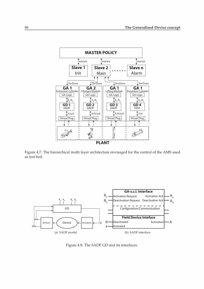
86 The Generalized Device concept
MASTER POLICY
Slave 1 Slave 2 Slave n
Init Main Alarm
GA 1Extraction Cylinder
GD 1SADF
PLANT
Do/Done Do/Done Do/Done Do/Done
req/ack req/ack req/ack
RA/R
D
A/a/d
GA Logic
Virtual Plug
GA 2Changer Module
GD 2DADF
A/D/a/d
GA Logic
Virtual Plug
GA 1Lifting Module
GD 3DADF
A/D/a/d
GA Logic
Virtual Plug
GA 1Expulsion Cylinder
GD 4SASF
A/d
GA Logic
Virtual Plug
RA/R
DR
A/R
DR
A/R
D
Figure 4.7: The hierarchical multi layer architecture envisaged for the control of the AMS usedas test bed.
Device a
dASensors Actuators
GD
RA
RD
AA
AD
(a) SADF model.
GA-s.c.l. Interface
Activation Request Activation Ack
Con�guration/Communication
Field Device IntefaceDeactivated
Activated
Activation
Deactivation Request
RA
RD
ad A
AA
AD
Deactivation Ack
(b) SADF interface.
Figure 4.8: The SADF GD and its interfaces.

4.4. The Generalized Devices 87
State1
Device
deactivated Activation Request=1
Deactivation Request=1
Activated=1Deactivated=1
Activatio
n Request=1
Deactivatio
n Request=1
Deactivation Request=0Activation=0
State2
Device
in activation
Activation=1
State3
Device
activated
Activation Request=0Activation=1
State4
Device
in deactivation
Activation=0
Figure 4.9: FMS modeling the behavior of the SADF GD.
The behavior of the SADF device in nominal operating conditions (i.e., following initializa-tion) is modeled by the FSM depicted figure 4.9. Three relevant aspects have to be pointedout. (i) A positive polarity is assumed for all GD inputs/outputs, meaning that the logicalname assigned to each of them unambiguously identifies, in positive logic, the role it plays.(ii) A very simple, yet effective, handshaking protocol is here envisioned to guarantee propercoordination between the GA-specific logic and the GD. The former requests the execution ofa service by asserting either RA or RD, the latter notifies service completion by de-assertingthe request.1 (iii) The GA may request the GD to abort the execution of a service by simplyasserting the opposite request.The interface shown in figure 4.8(b) has the following structure:
1. GA - interface: this section represents the input/output section between the GD and theGA. It can be further decomposed in two subsections separating the standard interfacebetween the GD and the GA and the interface for the configuration parameter of theGD and its communications with the GA. In this pat GD embeds all command inputsfor the GD an the outputs that communicate the actual state of the GD. More in detail,the single acting GD will receive as command the Activation request signal to activatethe device and the Deactivation request signal to deactivate the device. Fore a majorclearness think to a single acting cylinder: this type of device is normally in a specificposition (i.e. retracted) and it will move into the opposite position (i.e. extracted) assoon as the actuation command is raised that is the device is activated by the Activationrequest. The Deactivation request signal cause the device to return in its initial position.The double acting GD will receive as command the Activation request signal to activatethe device, the Deactivation request signal to deactivate the device and the Stop signalto stop the device operations. The Activation request and Deactivation request signalhave the same function as for the single acting GD, the difference with single acting GDis the presence of the Stop signal: single acting devices have only two stable positionwhile double acting devices have the possibility to be blocked in any position. When thedouble acting GD receive the Stop signal it block the field device in the current position.For both devices the unique output of this section is the State signal used to communicatethe actual state in which GD is evolving.
1Referring to an IEC61131-3 FB implementation of the GD, this is possible defining

88 The Generalized Device concept
0, ’Deactive’
Legend: In the �gure is represented a Moore automaton.
The outputs are expressed as <Activation Command, State>.
The transitions are expressed as <RA, RD, Dective, Active,> where:
RA=Activation Request
RD=Deactivation Request
RA, RD=x, 1, 0
1, ’In activation’RA, RD, 1, 0
RA, RD, 1, 0
RA, RD, 0, 1
1, ’Active’
RA=x, RD, 0, 1
RA, RD, 1, 0
0, ’In deactivation’
RA, RD, 0, 1
RA, RD, 0, 1
RA, RD, x, x
RA, RD, x, x
State1 State2
State3State4
Figure 4.10: State diagram for the single acting GD with double feedback
Configuration/Communications: represents all the signals that can be used to configuresome parameters of the GD such as the number of feedback, the diagnostic timers, theinitial state etc. and all the signal that can be used by the GD to communicate with theGA such as alarm signals or a sensor state.
2. Field device interface: this section contains as inputs all the links to sensors and as out-puts the links to actuators of the device that manages. More in detail, for both singleand double acting GD, the inputs of this section are the signal Activated and the signalDeActivated which are the link to the sensors that indicates when the device is active ordeactivated (e.g. the position of the actuation mechanisms). For the single acting GD theoutput of this section is the signal Activation command which is the link to the uniqueactuation command of the single acting actuation mechanisms. When this signal is highthe device is activated while when this signal is low the device is deactivated. For doubleacting GD the outputs of this section are the Activation Request signal and the Deactiva-tion Request signal. With the combination Activation Request=1, DeactivationRequest=0 the device is activated, with the combination Activation Request=0, Deactiva-tion Request=1 the device is deactivated while with the combination Activation Request=0,Deactivation Request=0 the device is blocked in its actual position. The combination withboth request high is not permitted.
A more detailed structure of the single acting GD is shown in figure figure 4.4. The automatonof figure figure 4.10 is the automaton for the nominal operation of the GD; for simplicity it issupposed that an initialization procedure is performed before starting the nominal operation.This is necessary for bring the device in a known configuration; the nominal automata can thenstart from the initial state (State1 of figure) which corresponds to the initial known configu-ration of the device. In the state State1 the GD is deActivated with the Activation Requestat a low logic level and then can receive only the Activation request command; the Activationrequest cause the GD to evolve in the state State2 where the Activation Request is raised.

4.4. The Generalized Devices 89
0, ’Deactive’
RA, RD=x, 1, 0
1, ’In activation’RA, RD, 1, 0
RA, RD, 1, 0
RA, RD, 0, 0
RA, RD, 0, 0
RA, RD, 0, 1
1, ’In activation’
1, ’Active’
RA=x, RD, 0, 1
RA, RD, 1, 0
RA, RD, 0, 0
0, ’In deactivation’
0, ’In deactivation’
RA, RD, 0, 1
RA, RD, 0, 0
RA, RD, 0, 1
RA, RD, 0, 1
RA, RD, 0, 0
RA, RD, 0, 0
RA, RD, 1, 0
State1 State2
State3
State4State5
State6
Legend: In the !gure is represented a Moore automaton.
The outputs are expressed as <Activation Command, State>.
The transitions are expressed as <RA, RD, Dective, Active,> where:
RA=Activation Request
RD=Deactivation Request
Figure 4.11: State diagram for the single acting GD with double feedback
The device is then in activation; before the completely activation of the device it is expectedthat the sensors combination changes from Activated=0, Deactivated=1 to Activated=1, Deac-tivated=0 (State3) when active. At this point the device can only be deactivated by risingthe Deactivation request signal. If during the activation of the device (state State2) the Deac-tivation request signal is raised (and contemporary the Activation request signal is removed)the GD passes in the deactivation states (State4). When the device is in deactivation there isthe same behavior.For the control modeling this description is complete but in order to sim-plify the diagnostic it is necessary to introduce an automaton with 6 states instead of 4: thismodel is said to be Diagnostic Oriented and is depicted in figure figure 4.4. Before thecompletely activation of the device it is expected that the sensors combination changes fromActivated=0, Deactivated=1 to Activated=0, Deactivated=0 (State3) and then to Activated=1,Deactivated=0 (State4) when active. At this point the device can only be deactivated by ris-ing the Deactivation request signal; also for the deactivation sequence it is expected the samechanges in the sensors combination as for the activation sequence (states State5 and State6).It must be taken into account that the device activation (or deactivation) could require a lot oftime and this time is then necessary for the fault signal. With the 6 states model the introduc-tion of a complete diagnostic function is simplified respect to the 4 states model. The doubleacting GD can be implemented through an event-driven automaton which states generallyevolve like depicted in figure 4.12. In this case it is directly represented only the Diagnostic

90 The Generalized Device concept
Legend: In the �gure is represented a Moore automaton.
The outputs are expressed as <A, D, Stop, State> where:
A=Activation command
D=Deactivation command
The transitions are expressed as <RA, RD, Dective, Active,> where:
RA=Activation Request
RD=Deactivation Request
RA, RD=x, Stop=x, 1, 0
RA, RD, Stop, 1, 0
A, D,
’In deactivation’RA, RD, Stop, 0, 1
RA, RD, 0, 0
RA, RD, Stop, 1, 0
OR
RA, RD, Stop, 1, 0
A, D, ’Stopped’
RA, RD, Stop, 0, 0
A, D, ’Deactive’
A, D,
’In activation’
A, D, ’Active’
A, D,
’In deactivation’
A, D,
’In activation’
RA, RD, Stop, 1, 0
RA, RD, Stop, 0, 0
RA, RD, Stop, 0, 0
RA, RD, Stop, 0, 1
RA=x, RD, Stop=x, 0, 1RA, RD, Stop, 0, 1
RA, RD, Stop, 0, 0
RA, RD, Stop, 0, 0
RA, RD, Stop, 1, 0
RA, RD, Stop, 0, 1
OR
RA, RD, Stop, 0, 1
RA, RD, Stop, 0, 0
OR
RA, RD, Stop, 0, 0
RA, RD, Stop, 0, 0
OR
RA, RD, Stop, 0, 0
RA, RD, Stop=x, 0, 0
State1 State2
State3
State4State5
State6 State7
Figure 4.12: State diagram for the double acting GD with double feedback
Oriented model. For the double acting GD is possible to make the same considerations as forthe single acting GD but with some modifications. Instead only one actuation command inthis case there are both the Activation Request signal and the Deactivation Request signal andin addition to the Activation request and Deactivation request signals there is also the Stopsignal. In the figure figure 4.12 is depicted the response of the GD to the different requests.The two automaton are almost identical, the unique practical difference is the presence of thestate State7 in the automaton of double acting GD. The GD is in this state when the actuationmechanisms is stopped between the two active and deactivated positions by rising the Stopsignal. In this state the device passes also during the direct changes between activation anddeactivation procedures to avoid the possible Activation Request=1, Deactivation Request=1combination during the transitions.
The two presented automatons represents the GD behavior in the double feedback case: thesemodels remains the same also in the case of single feedback or no feedback simply modifyingthe conditions of transition. The sensors that are not present must be substituted by a timerwhich drive the automaton evolution at the same way as the sensor signal. However it is notnecessary to design a GD for each feedback typology but only two GD must be designed thatare the single acting and the double acting GDs: using the configuration signals introducedearly, is possible to configure the GD for the operation as single, double or without feedback.

4.5. Fault diagnosis functionalities 91
TIMER>Clock
LD
zero
U/D’
E
Ad’a+A’da’
T
0
Timeout
(a) A simple and common ap-proach to fault diagnosis.
DECODER
I1
I3
I2
O1
O3
O2
A
a
d
En
TIMER>Clock
LD
zero
U/D’
E
DerivativeA
MUX
I0
I1
z
sA
O4
O6
O5
O8
O7
fd
S.A.F.
OK
OK
fA
S.A.T.
fa
S.A.T.
fa
S.A.F.
fA
S.A.F.
fd
S.A.T.
0
OK Correct !nal state
LEGEND
Stuck At False
Stuck At TrueS.A.T.
S.A.F.
Sensor Activated Faultfa
Sensor Deactivated Faultfd
fA
Actuator Fault
Timeout
TD
TA
(b) A refined approach to fault diagnosis with activation deactivationtimers.
Figure 4.13: Fault diagnosis approach.
4.5 Fault diagnosis functionalities
The presented approach gives the possibility of easily embedding within the GD also diagnos-tic functionalities. Clearly the diagnosis cannot be effectively performed unless consideringthe dynamic of the controlled device. A conceptual scheme of a simple and commonly usedapproach, envisaging a similar time for device activation and deactivation (TA = TD = T), is de-picted in figure 4.13(a). A timer is exploited to deal with the device dynamics. When the fielddevice is operating as expected in steady state conditions, that is when the inputs from sensorscoherently reflect the condition established by the actuator, the Load input of the timer preventsthe assertion of output (Timeout) devoted to signaling a (really generic) faulty behavior of thedevice. Upon activation or deactivation of the device, the timer starts its countdown. When thetimer expires (the zero output becomes true), and the generic fault message is asserted. Thisapproach, completely ignoring the cause-effect relationship existing between A and a, d, hastwo drawbacks: a faulty behavior of either sensor is reported with a T delay; an unexpectedbouncing of either sensor at a frequency less than 1/T is undetectable; unexpected, yet persist-ing, temporary configurations of either a or d, each lasting less than T, are undetectable. Animprovement may be addressed by considering the conceptual scheme of figure 4.13(b). Thecause-effect relationship between A (cause) and a, d (effects) must be taken into account. TheLoad input of the timer is driven by the derivative of A; at any slight variation of A the timerstarts its countdown. The decoder has been introduced to allow the detection of the faultysensor/actuator. When the timer expires (zero output becomes true), the decoder is enabledand the correct diagnostic information is generated. A MUX, driven by A, is used to select thecorrect time: if A=1 the device is activated and then, the activation timer TA must be selected,otherwise, if A=0, the device is deactivated and the deactivation timer TD must be used. Thelast proposed method, allow to solve all the drawbacks of the method of figure 4.13(a). It is im-portant to emphasize that the use of timers is exploited also to deal with the problem of image

92 The Generalized Device concept
d=1, a=1 d=1, a=0 d=0, a=0 d=0, a=1 d=1, a=1 d=1, a=0 d=0, a=0 d=0, a=1
Timeout = 1Timeout = 0
State
Device
activated
(A=1)
Device
deactivated
(A=0)
Device
in activation
(A=1)
Device
in deactivation
(A=1)
1
2 3 4
OK
OK
Instable state
Stable state
Initial stable state
Correct !nal stable state
LEGEND
a=0d=1
A=0 1
A=1
A=1
21
The actuation command is raised.
The device starts its movement
3
The device continue its movement
4 OK
The device has reached the active
state before the timer expiration
a=0d=0
a=1d=0
Figure 4.14: The SADF GD state space: state evolution during an activation cycle in absence offaults.
persistence: any decision must be performed just if the sensors configuration is a stable oneand not just a spurious transient configuration, an exhaustive discussion of this problem canbe find in [55]. Below, we consider a Structured Text (ST) implementation of the approach offigure 4.13(b); obviously, the methodology is independent of the programming language used.Suppose that the Timeout variable is generated as Timeout:=(DeviceTimer=0). The variableDeviceTimer is initialized at the correct value consistently with the value of A and is decreasedat regular time intervals (a Clock variable, synchronized with the system time, can be used tothis purpose). When the countdown ends, the Timeout variable becomes true.Note that the diagnosis is not performed for the whole duration of the activation/deactivationcycle. These cycles have a duration approximated by the activation/deactivation times whichmay be long time intervals. Therefore it may take a long time before a fault is detected. Toimprove the method, two different timers can be used: the first to monitor the duration of thetotal cycle whilst, the latter, to check if the device has started the action. The diagnostic func-tion is active if the device is into a stable state (Device activated or Device deactivated) or ifthe timer expires during an activation/deactivation cycle. To enable the diagnosis when thedevice reaches a stable state, the DeviceTimer variable will be set to 0 (and the Timeout vari-able rises to 1) as soon as the device has complete an activation/deactivation cycle. In this way,it is possible to recognize both the so called “static faults” and the “dynamic faults”. Staticfaults are faults that appear when the device is in a stable state, while dynamic faults are faultsthat appear when the device is in a non-stable state (i.e. Device in activation or Device in de-activation). To explain the dynamic of the fault signals generation we will consider a SADFdevice that implements the control of a pneumatic piston. In figure 4.14 is depicted the acti-vation cycle of the device without faults. Initially, the device is deactivated i.e., the pneumaticpiston is completely retracted. The activation request forces the GD to move to the Device inactivation state; the activation command A is raised, DeviceTimer is set to TA and the Timeoutvariable becomes false. The piston starts moving toward the extracted position. Contemporary,the DeviceTimer is decremented to scan the execution time of the activation cycle. As soon asthe piston reaches the active position (a=1), the DeviceTimer variable is set to 0, the Timeoutvariable becomes true and the diagnosis is enabled. In the situation of figure 4.14 the device

4.5. Fault diagnosis functionalities 93
State
Device
activated
(A=1)
Device
deactivated
(A=0)
Device
in activation
(A=1)
Device
in deactivation
(A=1)
d=1, a=1 d=1, a=0 d=0, a=0 d=0, a=1 d=1, a=1 d=1, a=0 d=0, a=0 d=0, a=1
Timeout = 1Timeout = 0
1
2ACTUATOR
FAULT
Timeout
LEGEND
a=0d=1
A=0 1
21
The actuation command is raised
but the device is blocked.
The timer expires before the
completely activation of the device.
The correct fault signal is generated.
ACTUATOR
FAULT
a=0d=1
Figure 4.15: Dynamic fault detection in the SADF GD state space.
a=0 1d=1
Sensor Activated
switch to high level
State
Device
activated
(A=1)
Device
deactivated
(A=0)
Device
in activation
(A=1)
Device
in deactivation
(A=1)
d=1, a=1 d=1, a=0 d=0, a=0 d=0, a=1 d=1, a=1 d=1, a=0 d=0, a=0 d=0, a=1
Timeout = 1Timeout = 0
1a
1
Figure 4.16: Static fault detection in the SADF GD state space.
correctly reaches the extracted position, the sensors coherently reflect the condition establishedby the actuator and therefore, no faults have affected the device. In figure 4.15 is depicted thesituation in which the piston is blocked in the retracted position. At the activation request, Ais raised, the DeviceTimer variable is set to TA and Timeout becomes false. The piston, how-ever, is blocked in the retracted position. DeviceTimer is continuously decremented to scanthe execution time of the activation cycle. When the DeviceTimer variable becomes 0 (Timeoutbecomes true) before the activation of the device, the diagnosis is enabled allowing to generatethe correct fault signal. The above presented fault belongs to the dynamic fault class. Such asexplained before, also static faults must be considered; an example of static fault is depicted infigure 4.16. The pneumatic cylinder is retracted, the GD is in the Device deactivated state andTimeout is true. The diagnosis is therefore enabled. By means of a fault, the a signal becomes(wrongly) true; the correct fault signal is then instantaneously generated. In figure 4.17 are de-picted all the diagnostic information that is possible to generate using the proposed procedure,both for dynamic and static faults. It’s important to note that the configuration d=1, a=1 bothfor the Device in activation and the Device in deactivation states is depicted as unreachablestate. This is because the evolution toward the activated/deactivated state, is performed assoon as the a/d signal becomes true. Suppose that the piston of figure 4.17 is moving towardthe extracted position; suppose also that, during the movement, the sensor d get stuck to the
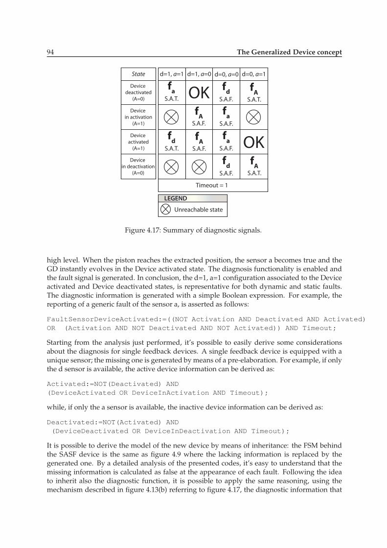
94 The Generalized Device concept
d=1, a=1 d=1, a=0 d=0, a=0 d=0, a=1
Timeout = 1
State
Device
activated
(A=1)
Device
deactivated
(A=0)
Device
in activation
(A=1)
Device
in deactivation
(A=0)
OK
LEGEND
fA
OKf
a
S.A.T.
fA
S.A.T.
fA
S.A.F.
fA
S.A.F.
S.A.T.
fd
S.A.T.
fd
S.A.F.
fd
S.A.F.
fa
S.A.F.
fa
S.A.F.
Unreachable state
Figure 4.17: Summary of diagnostic signals.
high level. When the piston reaches the extracted position, the sensor a becomes true and theGD instantly evolves in the Device activated state. The diagnosis functionality is enabled andthe fault signal is generated. In conclusion, the d=1, a=1 configuration associated to the Deviceactivated and Device deactivated states, is representative for both dynamic and static faults.The diagnostic information is generated with a simple Boolean expression. For example, thereporting of a generic fault of the sensor a, is asserted as follows:
FaultSensorDeviceActivated:=((NOT Activation AND Deactivated AND Activated)OR (Activation AND NOT Deactivated AND NOT Activated)) AND Timeout;
Starting from the analysis just performed, it’s possible to easily derive some considerationsabout the diagnosis for single feedback devices. A single feedback device is equipped with aunique sensor; the missing one is generated by means of a pre-elaboration. For example, if onlythe d sensor is available, the active device information can be derived as:
Activated:=NOT(Deactivated) AND(DeviceActivated OR DeviceInActivation AND Timeout);
while, if only the a sensor is available, the inactive device information can be derived as:
Deactivated:=NOT(Activated) AND(DeviceDeactivated OR DeviceInDeactivation AND Timeout);
It is possible to derive the model of the new device by means of inheritance: the FSM behindthe SASF device is the same as figure 4.9 where the lacking information is replaced by thegenerated one. By a detailed analysis of the presented codes, it’s easy to understand that themissing information is calculated as false at the appearance of each fault. Following the ideato inherit also the diagnostic function, it is possible to apply the same reasoning, using themechanism described in figure 4.13(b) referring to figure 4.17, the diagnostic information that

4.5. Fault diagnosis functionalities 95
is possible to give are the same as for the SADF device but, only the columns correspondingto the lacking information identical to false must be considered. More in detail, the proposedstrategy allow the detection of the “stuck at false”condition for the available sensor (it doesnot change its reading from 0 to 1 in a given amount of time when trying to move the deviceto the stable condition it monitors). For the same reason even the actuator faults cannot becompletely isolated: if the available sensor is the active-device sensor it is possible to detect the“stuck active”condition (signal a do not fall to 0 in time), if the available sensor is the inactive-device sensor it is possible to detect only the “stuck inactive”condition (signal d do not fall to 0in time). It is trivial to prove that for no feedback devices (where both sensors are replaced bya derived information), no diagnosis is possible because of the complete lack of information.Part of the ST code that implements the extraction cylinder GD is the following (in appendix Bis reported the entire code):
CASE (DeviceState) OFDeviceDeactivated:DeactivationRequet:=FALSE;IF (ActivationRequest) THEN
Activation:=TRUE;DeviceTimer:=ActivationTime;DeviceState:=DeviceInActivation;
END_IF;DeviceInActivation:IF (DeactivationRequest) THEN
ActivationRequest:=FALSE;Activation:=FALSE;DeviceTimer:=DeactivationTime;DeviceState:=DeviceInDeactivation;
ELSIF (Activated) THENActivationRequest:=FALSE;DeviceTimer:=0;DeviceState:=DeviceActivated;
END_IF;DeviceActivated:
ActivationRequest:=FALSE;IF (DeactivationRequest) THEN
Activation:=FALSE;DeviceTimer:=DeactivationTime;DeviceState:=DeviceInDeactivation;
END_IF;DeviceInDeactivation:
......END_CASE;
The ST code just presented simply implements the behavior modeled by the first three statesof the FSM of figure 4.9. It is possible to observe the implementations of the handshaking pro-tocol and the management of the DeviceTimer variable to allow the diagnosis of the anomalousconditions.

96 The Generalized Device concept
Load to
transport
Rotary Arm
Presence
sensor in testing
station
Distribution Testing
Vacuum
sensor
Figure 4.18: An example of high level fault.
4.6 Conclusions
In this chapter has been shown how it is possible to virtualize the hardware using the conceptof Generalized Device. This concept is based on the idea that the device a further categorizationof the devices can be performed on the basis of the number of feedback signals and actuationsignal command. The GDs represent therefore the standardization of an actuation mechanismaccomplished through the combination of an actuator, one or more sensors and basic controllogic. Starting from GDs concepts a hierarchical multilayer architecture for the control of au-tomated manufacturing systems has been presented. The emphasis has been particularly puton the diagnostic functionalities embedded within the GD entity. It has also been shown that,following an inheritance principle, starting from the SADF GD, the other typologies of GDscan be derived by means of simple extensions. The validity of the proposed approach has beenexperimentally ascertained by a case study derived from the automation field. The case studyenlightens how to implement GDs for the control of field devices typically used in automatedmanufacturing system. The major improvements due to the introduction of the GD compo-nents are twofold: (i) standardize logic control policies for basic field devices; (ii) introducestandard diagnostics functions for basic faults in field. Using this architecture we can dividethe fault in two level: low level fault and high level fault. A low level fault are faults on sen-sors or actuator and can be directly detects from the GD component. An high level fault arefault where two or more device are involving. An example of high level fault is the following:during the transport of a base from one station to the other, the load could fall down from therotary arm or the load can be efficaciously transported. In testing station there is a presencesensor, so when the load should arrives in testing station and presence sensor is FALSE it is notpossible to know if a fault on sensor presence occurs or the load fall down during transporta-tion. The situation is depicted in figure 4.18. The rotary arm is equipped with a vacuum sensorthat is been activated when a base is attached to the arm. Therefore, if the base is efficaciouslytransported, both the vacuum and the presence sensors must be at high logic level. A differentconfiguration of these sensors is an indication of fault. To detect this kind of fault it is neces-sary use information from different GD, but in this ways there is an architecture also for faultsdiagnosis.

Chapter 5A discrete event approach to faultdiagnosis in automated system
An important target for control systems, is the correct fault detection anddiagnosis and fault tolerant control. For this reason the concepts andtechniques of discrete event system theory are receiving increasing at-tention in industrial automation for control logic synthesis. Specifically,techniques from supervisory control, fault diagnosis, and fault-tolerantcontrol of discrete event systems can be employed to study propertiessuch as controllability, observability, and diagnosability, and to assist inthe synthesis of the monitoring and control logic. This chapter presentsa general and versatile approach for building structured formal modelsof complex automated systems in order to facilitate their control and di-agnosis, and it takes in consideration active fault tolerant control usingtechniques from discrete-event system theory.
5.1 Formal verification in industrial automation
Verification and validation (V&V)is the process of checking that a product, service, or systemmeets specifications and that it fulfills its intended purpose. Verification is a quality controlprocess that is used to evaluate whether or not a product, service, or system complies with reg-ulations, specifications, or conditions imposed at the start of a development phase. Verificationcan be in development, scale-up, or production. This is often an internal process. Validationis quality assurance process of establishing evidence that provides a high degree of assurancethat a product, service, or system accomplishes its intended requirements. This often involvesacceptance of fitness for purpose with end users and other product stakeholders.In software engineering, software testing, and software engineering, Verification and Valida-tion is the process of checking that a software system meets specifications and that it fulfils itsintended purpose. It is normally part of the software testing process of a project. With regardto the application of software engineering methods to control problems, an important role is
97

98 A discrete event approach to fault diagnosis in automated system
played by those methods that have as the major goal the construction of correct and reliablesystems, by means of analytical and mathematical-based languages, reasoning techniques andformal tools for the specification and verification of software systems. This notations and tech-niques are called formal methods, since both their syntax and semantics are supported by precisedefinitions, in contrast to those methods that puts more emphasis on the syntactical aspects ofthe description language, but define the semantics in an informal way. This notations and tech-niques are called semi-formal method. Formal methods represents therefore a way to eliminateambiguities in the description of a computational system, like a control logic in an industrialautomated system. and its desired properties, by means of a formal specification and then toapply reasoning procedure to reveal inconsistencies, incorrect behavior and flaws in the speci-fication of the system by means of formal verification procedures.The formal specification of an industrial system include the description of behavioral prop-erties, but also non-behavioral aspects like requirements real-time constraints or architecturaldesign. Specification methods that put particular emphasis on behavior are, for example, thosebased on tools and notations derived from DES theory, like automata, Petri Nets and State-charts. Statecharts is a notation develop to describe state diagram to describe the behavior ofsystems. State diagrams require that the system described is composed of a finite number ofstates; sometimes, this is indeed the case, while at other times this is a reasonable abstraction(see [41] and [42] ). In fact, the main field for the application of formal methods is that of reac-tive systems, where safety and real-time constraints are the major requirements, and the mostproper way to specify the behavioral properties of a reactive system is in terms of its compu-tational states and its response to events. Other formal methods, adopting a wide variety ofnotations and mathematical frameworks (i.e. sets, relations, functions, etc.) are: Z ([84]), VDM([53]), Temporal Logic ([75]).Model checking is a method to verify that a desired property holds for a finite state model of asystems performing an exhaustive states space search, which is guaranteed to terminate sincethe space is finite. Of course, the major problem in model checking is to define algorithms anddata structures that can manage efficiently large state spaces. In the just case, properties tocheck are expressed in a certain kind of temporal logic (Linear Temporal Logic or LTL, Compu-tation Tree Logic or CTL) while the system is modeled as a finite state transition system. Thesearch procedure then checks if the given state transition system is a model for the specification.Modal and temporal logics, which are formalisms to state requirements or safety relevant prop-erties of systems, although they are usually not considered as specification languages. Most ofthe presented languages are designed less with the authoring or communication aspect, andmore with the algorithm or tool aspect in mind: concrete syntax for temporal logic is oftensimplistic, tailored to some particular tool (like a model checker), and lacks the high concen-tration of syntactic sugar found in specification languages. Because there is a huge numberof temporal logic dialects, we only present the main families and common principles. This hasthe practical advantage that many properties (like satisfiability or the model checking problem)are decidable and can be checked automatically by tools. At the same time, temporal logics areoften sufficient to express many interesting requirements that can be imposed on a system. Thetwo main applications of temporal logics in software or system development are the generationof runtime assertions (in this context often called runtime monitors) and static verification bymeans of model checking. The main characteristic of both modal and temporal logics are thebuilt-in notions of states (or worlds) and transitions between states. The decision whether amodal formula is true is always made in the context of a particular active state. Temporal lan-guages provide larger varieties of modal operators, for instance to talk about states reachablein more than one step from the current state.
5.2. A DES approach for formal verification 99
Linear Temporal Logic (LTL, see [75])has been proposed in the late 1970s for the verification ofcomputer programs. It treats the “future” as a linear computation path consisting of discretestates. This means that propositions in LTL are always interpreted over individual paths. Incase of non-determinism, in which the space of possible program executions has the form of atree rather than a single linear path, an LTL formula is considered true if and only if it holds onall possible execution paths of the program: paths are implicitly universally quantified. Thisis the main difference between LTL and the alternative Computational Tree Logic, in whichexplicit universal and existential path quantifiers exist.Computational Tree Logic (CTL, see [75]) and CTL model checking were invented in the early1980s (see ). CTL is a branching-time logic and considers the “future” of program executionsas a tree (in contrast to LTL), thus making non-determinism directly observable by formulae.Such computation trees can be derived, e.g., from automata or Kripke structures by designatingsome state as the initial state and unfolding the structure into a (possibly infinite) tree with thedesignated state at the root. This tree shows all of possible executions starting from the initialstate.
5.2 A DES approach for formal verification
Designing control logic that provably satisfies given specifications is a problem of formal ver-ification. Industrial automated systems are very complex systems so for these systems is achallenging task. In chapter 3, chapter 4 and recent work in industrial automation has fo-cused on the concepts of modularity and reusability of the control logic; see, e.g., [11, 27, 94].To achieve all these objectives, the concepts and techniques of discrete-event system theoryare receiving increasing attention in industrial automation for control logic synthesis. Specif-ically, techniques from supervisory control, fault diagnosis, and fault-tolerant control of dis-crete event systems (see [17], [79], [97] and [70]) can be employed to study properties suchas controllability, observability, and diagnosability, and to assist in the synthesis of the mon-itoring and control logic; see, e.g., [43, 76, 62]. One of the earliest and most useful methodsis modular control (see [21]), this method involves designing multiple supervisors as opposedto centralized supervisor. Each supervisor implementing a portion of he control specification.All of these techniques however presume the availability of a complete formal model of thesystem; building such a model is a difficult task due to its dependence on deep knowledge ofthe system components and their physical coupling. To tackle the complexity of modeling theoverall system in a monolithic manner, researchers have considered decentralized approaches[81] or decomposition methods [29]. In [74] and [81] is proposed a model to fault diagnosis onmanufacturing systems. These works exploit the modularity of the model to avoid state explo-sion, nevertheless the complexity is avoided also using a fault-free-model. On the contrary themodularity should be exploited to deal with simpler models in which it is possible to definepost-fault behavior so that the precision of the FDI is improved and the strategy to counteractthe faults or to safely react can be formally defined. In the next sections will show a method-ology to develop a general and versatile approach for building structured formal models ofcomplex automated systems in order to facilitate their control and diagnosis using techniquesfrom discrete-event system theory. For this purpose, we present a methodology for building ina modular manner the complete model of a complex automated system starting from individ-ual components and their physical coupling. We employ finite-state automata as our modelingformalism. We propose a hierarchical decomposition that separates the control logic into high-level control actions (i.e., what to do) and low-level control actions (i.e., how to do it), coupled
100 A discrete event approach to fault diagnosis in automated system
through an interface. This hierarchical decomposition enables reusability of generic modelsfor low-level components. The low-level models incorporate low-level control actions as wellas fault detection logic for component faults. This fault detection logic requires modeling thefaulty behavior of the components in addition to their fault-free behavior.
The focus of this work is on model-building at the lower level of the proposed hierarchy.We start from generic fault-free models of low-level components such as actuators and sen-sors. In order to capture physical constraints among these low-level components in a givenautomated system, we propose the notion of physical constraint automaton, which is then cou-pled with the generic component automata by parallel composition. This approach achievesthe desired characteristics of modularity, composability, and reusability. We show how faultybehavior can be gradually incorporated into the model in a modular manner by enhancing thegeneric component models to include faults and by adjusting the associated physical constraintautomata in a manner that captures the effects of these faults on the physical coupling. As aconsequence, the entire faulty behavior is obtained by parallel composition of the individualfaulty models.
5.2.1 Architecture for supervisory control in industrial automation
In complex automated systems such as manufacturing systems, it is imperative to design thesupervisory controller and hence the control logic to achieve modularity and reusability. Asdiscussed in chapter 3 and chapter 4 a crucial point in this regard is the separation of actua-tion mechanisms from control policies, in order to hierarchically manage the plant. In otherwords, control should be viewed as the composition of: (i) a set of basic actions; and (ii) a set ofcoordination policies for the execution of these actions. This is the approach adopted and fur-ther elaborated in chapter 3. Designing the control logic using a hierarchical strategy supportscomponent interoperability and reusability and facilitates diagnostic and reconfiguration. Ourproposed hierarchical architecture is based on this approach and it is depicted in figure 5.1.This architecture consists of three levels:
• High level: This level embeds the control policy of the system; this policy is structuredas sequences of activation and deactivation commands for the lower levels. Note thatthere are no direct actuation commands and that only coordination sensors can appear asphysical signals.
• Interface: This level contains all the information necessary to let the high level commu-nicate with the low level.
• Low level: This level contains the basic control loops for single devices which implementthe actuation mechanisms.
A related hierarchical architecture is proposed in [58] [56] [57], where the focus is on the mod-ular verification of safety and nonblocking properties using local components and their inter-face, in the context of supervisory control problems. In this architecture (called HierarchicalInterface-based Supervisory Control) a system is decomposed into one high level subsystemand multiple low level subsystem which communicate between a well-defined interface. Ifeach subsystems and its interfaces satisfies certain local condition, then the global controllableand nonblocking properties can be guaranteed. The focus of this work is on the modelingmethodology rather than on the efficient verification of safety and nonblocking properties.We aim for generic low-level component models that are reusable, leaving to the high levelmodel application-dependent issues regarding “what to do” and “ when to do it”. Actuation

5.2. A DES approach for formal verification 101
High level(GH1, ΣH1)
Interface 1(GI1, ΣI1)
Device 1
Physical Plant
Low level 1(GL1, ΣL1)
Interface 2(GI2, ΣI2)
Device 2
Low level 2(GL2, ΣL2)
Interface 1(GIn, ΣIn)
Device n
Low level 1(GLn, ΣLn)
Figure 5.1: Hierarchical architecture.
mechanisms used to implement the desired high-level actions deal with “how to do it” issues,which are dependent on the low-level physical constraints. In this approach, the models of thelow-level components are application-independent and thereby reusable. Analyzing commonclasses of sensors and actuators that equip an automated manufacturing system, we can definegeneral categories of low level devices on the basis of the number of actuation mechanisms,e.g., single or double acting, and on the basis of the number of feedback signals, e.g., double,single, or no feedback; this characterization is presented in chapter 4. To ensure reusability ofthe low level components, we require that they have a a standard structure and also a standardset of input/output commands. This is where the interface, the middle level of the architec-ture, comes in. Its role is to map the high level commands into the low level commands. Allthe components of the architecture can be modeled as finite-state automata (indicated by thesymbol G in figure 5.1) over given event sets (indicated by the symbol Σ in Fig. 5.1). In order toensure the desired properties of modularity and reusability for the architecture, the followingassumptions are made:
ΣH1 ∩ ΣLn = ∅; (5.1)
ΣH1 ∩ ΣIn 6= ∅; (5.2)
ΣIn ∩ ΣLn 6= ∅; (5.3)
ΣLi ∩ ΣLj = ∅; (5.4)
GLi ∼ GLj . (5.5)
Equations (5.1), (5.2) and (5.3) ensure the separation between the control policy and the actu-ation mechanisms, while equation (5.4) guarantees the modularity and reusability of the lowlevel control/diagnosis logic. Controlled devices are modeled as isomorphic automata (withsymbol ∼ in 5.5 we indicate same structure) and hence their control and monitoring softwarecan be reused.

102 A discrete event approach to fault diagnosis in automated system
DA DA DA
D A
f fd0 d1, f fa0 a1,
10 00 01
f f0 1,
RAC0
RAC1
Figure 5.2: Illustrative example: Single acting device.
5.2.2 Model building methodology
To describe the architecture of figure 5.1 we start from the low level. This level associatesseveral low levels and their interfaces with the high level, according to the physical devicescomprising the system. In the next section will describe an approach to building automatamodels for a generic low-level device. The desired model is the composition of automata mod-els of hardware components (actuator and sensors) and models of logic components (controllogic, monitoring logic, and logic constraints as timers). The objective of this approach is toembed in the low level not only the low-level supervisory logic, but also the diagnostic logic inorder to (i) achieve reusable software as the low level devices are application-independent; and(ii) send to the high level the smallest amount of diagnostic information possible as explainedin chapter 4. Starting form a single acting cylinder example shown in figure 5.2 it will clarifythese crucial. This device has two end-of-stroke: sensors: sensor A signals when the device isin the activated position and sensor D signals when the device is in the deactivated position.Initially, the device is deactivated, that is, the pneumatic piston is completely retracted. Thedevice is driven by the actuation command AC . When AC is observed to be high, the devicemoves from left to right unless it was already in the rightmost position (activated). Likewise,when AC is observed to be low the device moves from right to left, again unless it was alreadyat the leftmost position (deactivated). Even this simple device can be affected by six differentfault scenarios, each sensor and the actuator can be stuck high, symbols fa1, fd1, f1, or stucklow, symbols fa0, fd0, f0, respectively for sensor A, sensor D, and the actuator. On the devicecan be occur multiple faults, but on each sensors or actuator only one fault at time, this meanwe can have 8 possible combinations of three faults in the worst case: {fa0, fd0, f0}, {fa1, fd0,f0}, {fa0, fd1, f0}, {fa0, fd0, f1}, {fa1, fd1, f0}, {fa1, fd0, f1}, {fa1, fd1, f1}, {fa0, fd1, f1}.When we consider fault on sensor or actuator we consider a physical fault on the component,or a fault on the wire connection between sensor and hardware control logic like PLC or mi-crocontroller, because from control logic point of view it’s not possible to distinguish if a faultoccurs on the component or if a fault occurs on line connection, for example if on a sensor thereis an hardware fault to stuck low the logic out of the sensor, or there is a line disconnection ofsensor out on the control logic there is the same effect, it is not possible to distinguish the causeof the fault; With the notation fa0, for example, we do not distinguish if fault involves sensorcomponent or sensor connection line to control logic.

5.2. A DES approach for formal verification 103
Sensor A
Physical Plant
Sensor D Actuator
Timer
RA0, RA1 RD0, RD1
RAC0, RAC1
Control + Diagnosis
Physical Constraints
Au,Ad Du,Dd
ACu, ACd
Control
Figure 5.3: Physical and logic components of the low level of the architecture.
5.2.3 Low level
Starting from a single acting cylinder example shown in figure 5.2 it will see the methodologyfor building the model in nominal condition and fault condition. Low-level component modelscan be constructed by the interconnection of physical components (actuators and sensors) andlogical components (control logic, diagnostic logic and timing logic) as shown in figure 5.3. Westart constructing a low-level component by first introducing nominal models for the physi-cal components as shown in figure 5.4. Sensor A has two steady states A0 and A1; in thesestates we can have two observable events RA0 and RA1 indicate if the sensor is read to below or high respectively, while unobservable events Au and Ad indicate that the sensor outputchanged from low to high, or high to low, respectively. Sensor D is modeled in an analogousmanner (we can define the same events only change label A with label D). The actuator alsohas two steady states Act0 (retracted) and Act1 (extended); unobservable events RAC0 andRAC1 correspond to the movement of the device in one direction or the other. From the pointof view of the controller these events are unobservable because the controller cannot observethe movement of the device, it can only read sensor states. Events ACu and ACd are the com-mands used by the control logic to switch the position of the actuator and hence are observableand controllable, these events can be associate to command send from control logic, for exam-ple command Act:=1 and Act:=0If the beginning the actuator is in state Act0 to move the actuator the control logic send the
A0 A1
Ad
AuRA0 RA1
(a) No fault model GL,Anf .
D0 D1
Dd
DuRD0 RD1
(b) No fault model GL,Dnf .
Act0 Act1
RAC0 ACu
ACd
RAC1
ACuACd
(c) No fault model GL,Actnf .
Figure 5.4: Nominal models of the sensors and actuator.
command Act:=1 that generates event ACu and actuator will evolve in state Act1 and fromthis state control logic can send a command Act:=0 that generates event ACd to move actu-ator in the opposite direction. It is possible to not have the alternate sequence of commandAct:=0, Act:=1, this because can happens that after control logic send command Act:=1
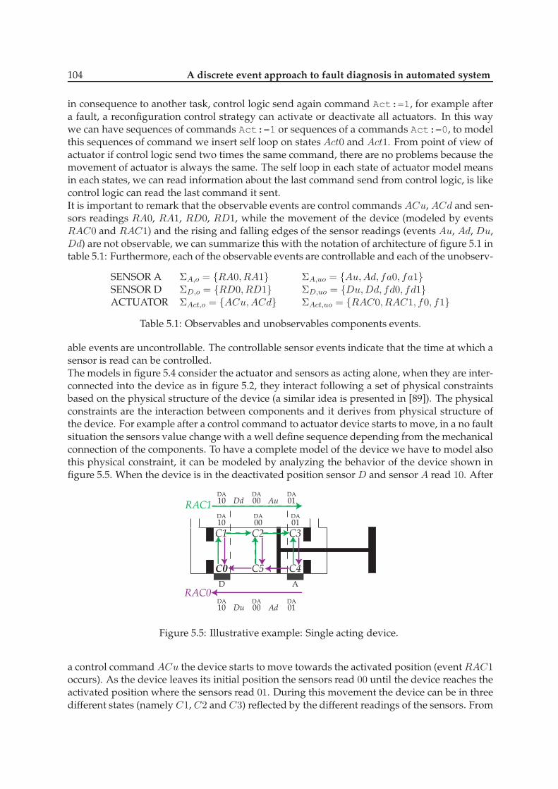
104 A discrete event approach to fault diagnosis in automated system
in consequence to another task, control logic send again command Act:=1, for example aftera fault, a reconfiguration control strategy can activate or deactivate all actuators. In this waywe can have sequences of commands Act:=1 or sequences of a commands Act:=0, to modelthis sequences of command we insert self loop on states Act0 and Act1. From point of view ofactuator if control logic send two times the same command, there are no problems because themovement of actuator is always the same. The self loop in each state of actuator model meansin each states, we can read information about the last command send from control logic, is likecontrol logic can read the last command it sent.It is important to remark that the observable events are control commands ACu, ACd and sen-sors readings RA0, RA1, RD0, RD1, while the movement of the device (modeled by eventsRAC0 and RAC1) and the rising and falling edges of the sensor readings (events Au, Ad, Du,Dd) are not observable, we can summarize this with the notation of architecture of figure 5.1 intable 5.1: Furthermore, each of the observable events are controllable and each of the unobserv-
SENSOR A ΣA,o = {RA0, RA1} ΣA,uo = {Au,Ad, fa0, fa1}SENSOR D ΣD,o = {RD0, RD1} ΣD,uo = {Du,Dd, fd0, fd1}ACTUATOR ΣAct,o = {ACu,ACd} ΣAct,uo = {RAC0, RAC1, f0, f1}
Table 5.1: Observables and unobservables components events.
able events are uncontrollable. The controllable sensor events indicate that the time at which asensor is read can be controlled.The models in figure 5.4 consider the actuator and sensors as acting alone, when they are inter-connected into the device as in figure 5.2, they interact following a set of physical constraintsbased on the physical structure of the device (a similar idea is presented in [89]). The physicalconstraints are the interaction between components and it derives from physical structure ofthe device. For example after a control command to actuator device starts to move, in a no faultsituation the sensors value change with a well define sequence depending from the mechanicalconnection of the components. To have a complete model of the device we have to model alsothis physical constraint, it can be modeled by analyzing the behavior of the device shown infigure 5.5. When the device is in the deactivated position sensor D and sensor A read 10. After
DA DA DA
D A
10 00 01
C0
C1
C5
C2
C4
C3
RAC0DA DA10 01
DA00 AdDu
RAC1 DdDA DA10 01
DA00 Au
Figure 5.5: Illustrative example: Single acting device.
a control command ACu the device starts to move towards the activated position (event RAC1occurs). As the device leaves its initial position the sensors read 00 until the device reaches theactivated position where the sensors read 01. During this movement the device can be in threedifferent states (namely C1, C2 and C3) reflected by the different readings of the sensors. From

5.2. A DES approach for formal verification 105
each states the device can change the movement direction, for this reason are presented statesC0, C4 C5, in these states the sensors value in the device have the same respective readings asin C3, C2 and C1. In figure 5.6 is shown the Physical Constraint Automaton (PCA) that modelsthese constraints. The initial state C0 corresponds to device in deactivate position and RAC0movement. During an activation sequence (from state C0 to state C3) sensors DA evolve inwith a well define sequence depending from its structure, sensors evolve from reading 10 toreading 01. From state C1 to state C2 sensor D evolves from a value 1 to value 0 in accordingwith an event Dd, and from state C2 to state C3 sensor A evolves from value 0 to value 1 inaccording with Au.The PCA automaton captures all the physical connection between the components, it is impor-
C0
C1Au
AdDu
Dd
RAC0
C5
C2
C4
C3
RAC1 RAC0RAC1 RAC0RAC1
Figure 5.6: Physical Constraint Automaton (PCA) GL,PCA
tant to remark events RAC0 and RAC1 are not control command, but they are the movementof the device, this model is complete independent from control logic. All events in this modelare unobservable events, these events interact with sensors and actuator model that generateobservable events, as it is shown figure 5.3. Control logic can observe control commands ACu,ACd, and events of sensors value (RA0, RD1 etc.), but control logic can not see movement ofthe device, i.e. events RAC0 and RAC1 are unobservable for control logic. Events Au, Du, etc.are not observable because control logic can only acquire sensor value. The PCA automatonof figure 5.6, is like a component that receive as input the events of the device movement fromactuator model, and generate the correct events to change sensors states. In section 5.2.4 thisapproach to encapsulate unobservable events will help to model the components fault model.Composing the automata of sensors and actuator in figure 5.4 and PCA automaton in figure 5.6
we obtain the automaton in figure 5.7 (12 states 62 transitions).Remark The automata models of figure 5.7 do not includes any control logic, but the nominalactivation and deactivation sequence of the device that could be implemented by a controlleris shown in blue (path from 1 to 8). Of course the automaton can perform other sequence de-pending on the actual control logic employed, or as will be possible see in next sections (see ),in the case due to the occurrence of faults.Remark The operation of the device is characterized by three sources of information, readingsfrom the two sensors and commands to the actuator. This information indicates the state of thedevice. The state of the device can be changed by a new control command (events ACu,ACd)that forces a change in the states of the sensors (events Au,Ad,Du,Dd) through the constraintautomaton PCA. The self loops of the automata in figure 5.7 and can be thought of as “outputs”emitted from a given state in much the same manner as a Moore automaton.The state of the device can be change after a new control command, for example in figure 5.8,
transition 1 is a transition generates after a new control command ACu from control logic, thistransition let’s evolve the state from [RD0 RA1 ACd] to [RD0 RA1 ACu]. Also if the device donot change its sensors configuration, the device is in a new state because is changed the controlcommand. This changes will force the actuator to move ( event RAC1 is generated). This event
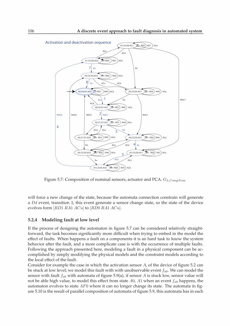
106 A discrete event approach to fault diagnosis in automated system
A0,C0,D1,AC1
A1,C4,D0,AC1
A0,C0,D1,AC0
A1,C4,D0,AC0
A1,C3,D0,AC1
A1,C3,D0,AC0
A0,C5,D0,AC1
A0,C5,D0,AC0
A0,C2,D0,AC1
A0,C1,D1,AC1
A0,C2,D0,AC0
A0,C1,D1,AC0
Dd
RAC0
ACd
ACd
ACu
RAC0
RD0
Ad
Au
ACu
ACd
Du
RA0
ACu
ACd
RAC0
ACu
Du
ACu
RA0RD1
Ad
RD0
RAC1
RD0
RA0
ACu
RD1
ACd
ACd
ACu
RD1
ACu
RA0
ACd
RAC1 RAC1
ACd
RD0
RA0
ACu
RD0 RA1
ACu
ACd
RA0
Au
RA1
RA1
ACu
RD0
RA0
ACd
RA1
ACd
Dd
RD0
RD0
ACu
RD1
ACd
RA0
Activation and deactivation sequence
1
2
3
4
5
6
7
8
Figure 5.7: Composition of nominal sensors, actuator and PCA. GL,CompNom
will force a new change of the state, because the automata connection constrain will generatea Dd event, transition 3, this event generate a sensor change state, so the state of the deviceevolves form [RD1 RA1 ACu] to [RD0 RA1 ACu].
5.2.4 Modeling fault at low level
If the process of designing the automaton in figure 5.7 can be considered relatively straight-forward, the task becomes significantly more difficult when trying to embed in the model theeffect of faults. When happens a fault on a components it is an hard task to know the systembehavior after the fault, and a more complicate case is with the occurrence of multiple faults.Following the approach presented here, modeling a fault in a physical component can be ac-complished by simply modifying the physical models and the constraint models according tothe local effect of the fault.Consider for example the case in which the activation sensor A, of the device of figure 5.2 canbe stuck at low level; we model this fault with with unobservable event fa0. We can model thesensor with fault fa0 with automata of figure 5.9(a), if sensor A is stuck low, sensor value willnot be able high value, to model this effect from state A0, A1 when an event fa0 happens, theautomaton evolves to state AF0 where it can no longer change its state. The automata in fig-ure 5.10 is the result of parallel composition of automata of figure 5.9, this automata has in each

5.2. A DES approach for formal verification 107
A0,C0,D1,AC1
A0,C0,D1,AC0
A0,C2,D0,AC1
A0,C1,D1,AC1
Dd
ACu
ACu
ACu
RA0
RA0
RD1
ACdRD1
RAC1
ACu
RA0
RD0
RD1
RA0
1
2
3
STATE
Figure 5.8: States model of the system.
A0 A1
fa0
AF0
Ad
AuRA0 RA1
fa0
RA0
(a) Fault model of sensor A,GL1,Afa0.
D0 D1
Dd
DuRD0 RD1
(b) No fault model of sensorD, GL,Dnf .
C0
C1Au
AdDu
Dd
RAC0
C5
C2
C4
C3
RAC1 RAC0RAC1 RAC0RAC1
(c) (PCA) GL,PCA.
Figure 5.9: Composition of PCA automata, sensor D and sensor A fault model.
state only two self loop because in this composition we not consider actuator, but only sensorson the parallel composition. The automaton of figure 5.10 is the model of the device withoutmodel of actuator, the sequence of state in blue is the sequence of activation and deactivationsequence, in green is depicted the sequence of activation and deactivation when fault fa0 hap-pens. It’s possible to see that from each state fault fa0 can occurred and the system evolvesfrom nominal cycle of activation and deactivation sequence, to faulty cycle of activation anddeactivation. In the model there is a livelock, but this livelock is not a physical behavior of thesystem. When the fault fa0 occurs the device can move in the two directions, but sensor A hasalways low value and sensor D work in normal condition. The livelock is generated becausein our model we not considered that when a fault occurs, we do not have only a consequenceon the model of sensor, but the fault change the physical interaction between the component.When a sensor is stuck low from a physical point of view is like the device do not have thesensor. In this case if sensor A is stuck low, we can remodeling the device with only sensor D,and the device becomes the device of figure 5.11. The model of this device is composed by anautomata of 4 states, because now we can have only two sensors configuration, 10 configura-tion and 00 configuration, this model can be obtained, as it shown in figure 5.11(b), from modelof PCA automaton. If sensor A is stuck low the model has not to generate events Au and Ad,for this reason the model on sensor A when occurs fault fa0 evolves and remains in state AF0.

108 A discrete event approach to fault diagnosis in automated system
A0,C1,D1
A0,C5,D0
AF0,C5,D0
AF0,C1,D1
A0,C0,D1
AF0,C4,D0
AF0,C0,D1
AF0,C3,D0 A1,C4,D0
A0,C2,D0
AF0,C2,D0 A1,C3,D0
Au
RA1
RAC1
RA0
RA0
Ad
RA0
RAC1
fa0
fa0
RD0
RD0
RA0
RD1
Du
RAC0
RD0
RAC1
RA0
RAC0
RA1
RD0
RD1
Du
fa0
fa0
RAC1
RAC1
RAC0
RD0
RA0RD1
Dd
RA0
RAC0
RAC0
RD1
RD0
RA0 RD0
RAC1
RA0
RD0
Dd
fa0
RA0
RAC0
fa0
Activation and
deactivation sequence
Fault fa0
sequence
Livelock
Figure 5.10: Nominal and faulty model with livelock.
The PCA automaton do not reach states C3 and C4 but evolves only in states C0, C1, C2 andC5. If the fault occurs when the system is in states C3 or C4 the model has a livelock. Thislivelock is generated, as it is possible to see in figure 5.10, because now event Ad is not generatefrom sensor model, we have to considerate in the physical constraint automaton the new in-teraction between component. This new model is depicted in figure 5.12(c). This event (OutA)must be considered also in the model of the sensor, for this reason sensor A it is the automata offigure 5.12(a), the parallel composition of automata of figure 5.12 is shown in figure 5.13. Themodel presented in figure 5.13 is the model of the device in no fault condition and fault condi-tion, the powerful of this approach is that the complete model of the system is generate fromparallel composition of simples automata. The effect of the fault can be considered as a localeffect on the component when fault happens, in this example the local effect of the fault is theself loop RA0 on the sensor model and the event OutA on the sensor model and on connectionconstrain model it’s the effect of the fault on the interaction of the component, the completebehavior of the system is generate by parallel composition of the model, and don’t be model,this is the powerful of this approach.Remark The fault has two consequences, a local consequence on the sensor modeled by the au-tomaton figure 5.12(a) getting stuck in state AF0 and a global consequence on the whole devicemodeled by PCA in figure 5.12(c)A sensor can fault in stuck high, in this case the device change its physical configuration asdepicted in figure 5.14. This case is similar with the case when sensor is stuck low. The phys-ical constraints are the same because there in no a different relation between the sensors, thedifferent condition fault is on sensor (now is stuck high) and also in this case the model hasnot to generate events Au and Ad, for this reason the model on sensor A when occurs fault fa1evolves and remains in state AF1 from state A0 or evolves in state AF1 with event OutA. ThePCA automaton do not reach states C3 and C4 but evolves only in states C0, C1, C2 and C5.With a stuck high fault on sensor A the PCA automaton has the same evolution of sensor stucklow, this because in PCA is captured the information of a sensor fault, and in sensor model is

5.2. A DES approach for formal verification 109
DA DA
D
fa0
10 00
DdRAC1
DA DA10 00
DuRAC0
DA DA10 00
A
RAC1
RAC0
(a) Mechanical configuration fault fa0.
C0
C1Au
AdDu
Dd
RAC0
C5
C2
C4
C3
RAC1 RAC0RAC1 RAC0RAC1
(b) New configuration of (PCA) with fault fa0.
Figure 5.11: Models of fault fa0.
A0 A1
fa0
AF0
Ad
AuRA0 RA1
fa0
RA0
AG0RA0
OutA
(a) Fault model of sensor A,GL,Afa0.
D0 D1
Dd
DuRD0 RD1
(b) No fault model of sensorD, GL,Dnf .
C0
C1Au
AdDu
Dd
RAC0
C5
C2
C4
C3
RAC1 RAC0RAC1 RAC0RAC1
OutA
(c) Physical Constraint Automaton with fault fa0,GL,PCAA
.
Figure 5.12: Composition of automata connection with sensor A fault model.
captured the information if sensor is stuck low or stuck high. In figure 5.15(a) is shown thecomplete model of sensor A it is possible to note the symmetry structure of the model.In figure 5.15(b) is depicted the model of sensor D. The model has the same structure of model
of sensor A, in this model there is event OutD which the dual means of event OutA. The modelof how changes physical constraints is reported in figure C.6, and figure C.7 in appendix C.When a fault on sensor D occurred, also the PCA automaton has been model with a new event(OutD), the new PCA automaton is depicted in figure 5.16. When sensor D is stuck low (orstuck high), the model of this device is composed by an automata of 4 states, because now wecan have only two sensors configuration, 00 configuration and 01 configuration, this model canbe obtained, as it shown in figure C.6(b), from model of PCA automaton. If sensor D is stucklow the model has not to generate events Au and Ad, for this reason the model on sensor Dwhen occurs fault fd0 evolves and remains in state DF0. The PCA automaton do not reachstates C0 and C1 but evolves only in states C2, C3, C4 and C5. In the model presented it is considerate only one fault, but on a device can occur multiplefault, sensor A and sensor D can be fault at the same time. The model building methodologyis complete modular and the same model of the components can be applied. The physicalconstraint automaton has to change because when two fault are possible we introduce a new
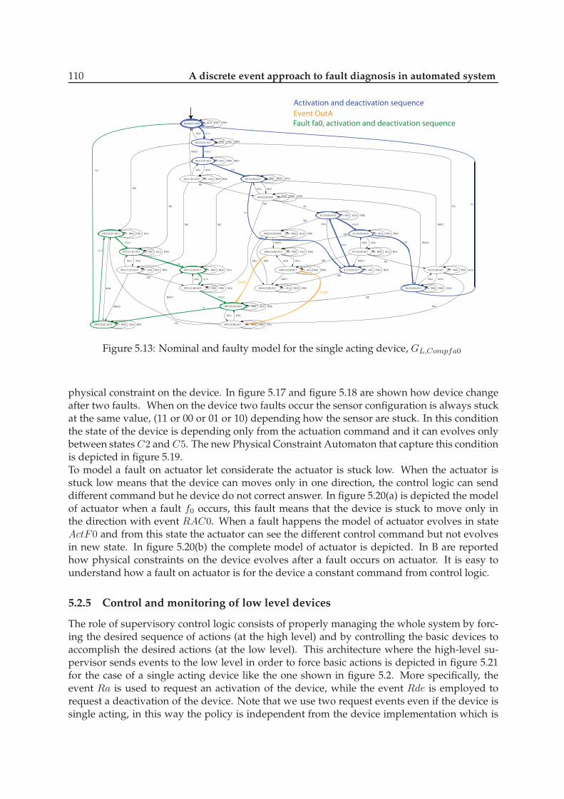
110 A discrete event approach to fault diagnosis in automated system
AF0,C0,D1,AC1
AG0,C3,D0,AC1
AF0,C0,D1,AC0
AG0,C3,D0,AC0
A0,C0,D1,AC1
A0,C0,D1,AC0
A1,C4,D0,AC1
A1,C4,D0,AC0
AF0,C2,D0,AC1
AF0,C5,D0,AC1
AF0,C2,D0,AC0
AF0,C5,D0,AC0
A0,C2,D0,AC1
A0,C5,D0,AC1
A0,C2,D0,AC0
AF0,C1,D1,AC1
AG0,C4,D0,AC1
A0,C5,D0,AC0
AF0,C1,D1,AC0
AG0,C4,D0,AC0
A0,C1,D1,AC1
A0,C1,D1,AC0
A1,C3,D0,AC1
A1,C3,D0,AC0
ACu
ACd
RA0
RAC0
fa0
RAC1
RD0
RA0
RD0
RA0
RA0 ACd
ACu
ACu
RD0
fa0
RD0
fa0
ACd
ACu
ACu
RAC1
ACu
ACu
fa0
ACd
ACd
Du
fa0
RD1
ACd
RA0
RD0
ACu
RD1
RD0
Dd
Du
ACuRA0 RA1
RD1
ACd
fa0
RA0
ACu
RD1
Ad
RD0RA0
ACd
ACu
ACu
Du
ACu
RA0
RAC0
RA1
ACd
RD0
ACd
ACd
RA0
RD0
RD0
RD0
ACu
RAC1
ACu
RAC0
ACu
ACdACu
Dd
Au
RAC1
RA0
fa0
RA0
RD0
ACu
RAC1ACd
RD0
ACd
RA1
RA1
RD0
ACd
RA0
Dd
RA0
RD1
ACu
OutA
fa0
fa0
fa0
ACd
RA0
RA0
ACd
ACu
ACd
fa0
Ad
fa0
ACd
ACu
Au
RD0ACu
RA0ACd
RAC0
RD0
Dd
Du
OutA
RA0
RD1
ACd
ACd
RD1
RA0
RAC1
ACd
ACu
RA0
ACu
RAC0
RD1
ACd
RAC0
Activation and deactivation sequence
Event OutAFault fa0, activation and deactivation sequence
Figure 5.13: Nominal and faulty model for the single acting device, GL,Compfa0
physical constraint on the device. In figure 5.17 and figure 5.18 are shown how device changeafter two faults. When on the device two faults occur the sensor configuration is always stuckat the same value, (11 or 00 or 01 or 10) depending how the sensor are stuck. In this conditionthe state of the device is depending only from the actuation command and it can evolves onlybetween states C2 and C5. The new Physical Constraint Automaton that capture this conditionis depicted in figure 5.19.To model a fault on actuator let considerate the actuator is stuck low. When the actuator isstuck low means that the device can moves only in one direction, the control logic can senddifferent command but he device do not correct answer. In figure 5.20(a) is depicted the modelof actuator when a fault f0 occurs, this fault means that the device is stuck to move only inthe direction with event RAC0. When a fault happens the model of actuator evolves in stateActF0 and from this state the actuator can see the different control command but not evolvesin new state. In figure 5.20(b) the complete model of actuator is depicted. In B are reportedhow physical constraints on the device evolves after a fault occurs on actuator. It is easy tounderstand how a fault on actuator is for the device a constant command from control logic.
5.2.5 Control and monitoring of low level devices
The role of supervisory control logic consists of properly managing the whole system by forc-ing the desired sequence of actions (at the high level) and by controlling the basic devices toaccomplish the desired actions (at the low level). This architecture where the high-level su-pervisor sends events to the low level in order to force basic actions is depicted in figure 5.21for the case of a single acting device like the one shown in figure 5.2. More specifically, theevent Ra is used to request an activation of the device, while the event Rde is employed torequest a deactivation of the device. Note that we use two request events even if the device issingle acting, in this way the policy is independent from the device implementation which is

5.2. A DES approach for formal verification 111
DA DA11 01
DdRAC1
DA DA11 01
DuRAC0
DA DA11 01
D fa1
A
RAC1
RAC0
(a) Mechanical configuration fault fa1.
C0
C1Au
AdDu
Dd
RAC0
C5
C2
C4
C3
RAC1 RAC0RAC1 RAC0RAC1
(b) New configuration of (PCA) with fault fa0.
Figure 5.14: Models of fault fa1.
hidden in the low-level control logic. When the device has accomplished the high-level requestit notifies the high level using event Aa (activation accomplished) and event Ade (deactivationaccomplished). The desired behavior for the controlled device is depicted by the automatonEL,ConNom shown in Fig. 5.22; this automaton is the low-level specification. The device is ini-tially inactive, when the high level asks for an activation it sends the event Ra which causes thecommand ACu to be sent to the actuator. After a given amount of time event RD0 signals thatthe device is not inactive anymore. After an additional amount of time event RA1 indicatesthat the device is activated. This fact causes event Aa that acknowledges the accomplishmentof the request to the high level. At this point the low-level control waits for a deactivation re-quest (event Rde). When this request arrives it starts the deactivation cycle which is dual to theactivation cycle. When the device is deactivated it generates the event Ade. The observabilityand controllability of the low level events are as defined previously, while the high level re-quest and answer events {Ra,Aa,Rde,Ade} are observable and controllable.Summarize the controllable and uncontrollable events set are: ΣA,c = {RA0, RA1}, ΣD,c ={RD0, RD1}, ΣAct,c = {ACu,ACd}ΣCon,c = {Ra,Aa,Rde,Ade,RA0, RA1, RD0, RD1, ACu,ACd}and the following uncontrollable event sets ΣA,uc = {Au,Ad, fa0, }, ΣD,uc = {Du,Dd} andΣAct,uc = {RAC0, RAC1}Composing the low-level specification in figure 5.22 with the nominal sensors, actuator andPCA models of figure 5.4 and figure 5.6, we obtain the controlled device model GL,DevNom
shown in figure 5.23(a). It is possible to note that figure 5.23(a) the automaton doesn’t have selfloop in the states, instead model without control in each states has self loop. From a physicalpoint of view the model without control is the model of the device, in each states the device hasa sensors configuration, and the last command sends to actuator, the control logic can acquirethe information on the sensors, and information on the last command send to actuator in eachtime. Let’s considered this part of code of control logic:
CASE DeviceState OFDeactive:IF (Ractive) THANActuator:=TRUE;DeviceState:=InActivation;END_IF;

112 A discrete event approach to fault diagnosis in automated system
A0 A1
fa0
AF0
Ad
AuRA0 RA1
fa0
RA0
AG0RA0
OutA
fa1
RA1
AF1
AG1
RA1
fa1
OutA
(a) Fault Model of sensor A,GL,Afa.
D0 D1
fd0
DF0
Dd
DuRD0 RD1
fd0
RD0
DG0RD0
OutD
fd1
RD1
DF1
DG1
RD1
fd1
OutD
(b) Fault Model of sensor D,GL,Dfd.
Figure 5.15: Models of sensor A and sensor D.
C0
C1Au
AdDu
Dd
RAC0
C5
C2
C4
C3
RAC1 RAC0RAC1 RAC0RAC1
OutD
Figure 5.16: Physical Constraint Automaton with fault fd0 or fault fd1, GL,PCAD.
.
.IF (SensorA) THANAactive:=TRUE;DeviceState:=Activated;END_IF;..END_
The construct CASE implements the automata, the variable DeviceState is the state of controlautomata, when it executes parallel composition between control and model of device is likethe physical operation that control acquire for example a sensor value, the control can read inany time a sensor value, this feature is implemented in the model by self loop with sensor con-figuration in each state. For example when control executes instruction IF (SensorA) Thenthe control loops on acquire sensor A value, and when it’s value is high the control executesthe code in THAN instruction, from a point of view of model this is equivalent to model control

5.2. A DES approach for formal verification 113
DA00
RAC1
DA00
RAC0
DA00
Dfa0
Afd0
RAC1
RAC0
(a) Mechanical configuration fault fd0and fa0.
C0
C1Au
AuDu
Dd
RAC0
C5
C2
C4
C3
RAC1 RAC0RAC1 RAC0RAC1
(b) New configuration of (PCA) with faults fd0and fa0.
Figure 5.17: Models of fault fd0 and fa0.
DA11
RAC1
DA11
RAC0
DA11
Dfd1
Afa1
RAC1
RAC0
(a) Mechanical configuration fault fd1and fa1.
C0
C1Au
AuDu
Dd
RAC0
C5
C2
C4
C3
RAC1 RAC0RAC1 RAC0RAC1
(b) New configuration of (PCA) with faults fd1and fa1.
Figure 5.18: Models of faults fd1 and fa1.
is in a state that generate event RA1 and device model evolves in a state with a self loop eventRA1, when control and device model are both in a state with RA1 events, parallel compositiongenerates event RA1 in complete model, and this event in complete model corresponding tosensor A value is high and control executes the THAN.The process of determining whether the control desired by EL,ConNom is actually achievablefirst requires defining the automaton Glifted
L,CompNom as GL,CompNom with self-loops added forevents in the set ΣEL,ConNom
\ΣGL,CompNom= {Ra,Aa,Rde,Ade}. The language generated by
GL,DevNom, L(GL,DevNom) ⊆ L(GliftedL,CompNom), can be shown to be controllable and observable
with respect toL(GliftedL,CompNom). Therefore, there exists a supervisorS such that S/Glifted
L,CompNom =GL,DevNom. EL,ConNom is an automaton realization of supervisor S.If we consider the models for the single acting device with fault fa0 (see fig. 5.12) composedwith the nominal controller in fig. 5.22, we obtain the controlled device model GL,Devfa0 infig. 5.23(b) from the parallel composition of models GL,Afa0, GL,Dnf , GL,Actnf , GL,PCA_A andEL,ConNom. Note that the automaton GL,Devfa0 in figure 5.23(b) has a deadlock due to the oc-currence of the fault fa0. Since sensor A cannot rise to true, this deadlock arises due to the factthat the controller will never know when the device has been activated. To avoid this dead-lock we consider a new logical model that considers also timing constraints. When the device

114 A discrete event approach to fault diagnosis in automated system
C0
C1Au
AdDu
Dd
RAC0
C5
C2
C4
C3
RAC1 RAC0RAC1 RAC0RAC1
OutD
OutA
Figure 5.19: Physical Constraint Automaton with fault on sensor A and sensor D.
Act0 Act1
RAC0 ACu RAC1
ACuACd
f0
f0
RAC0, ACu, ACd
ActF0
ACd
(a) Fault Model of actuator GL,Actf0.
Act0 Act1
RAC0 ACu RAC1
ACuACd
f0 f1
f1f0
RAC0, ACu, ACd
ActF1ActF0
ACd
RAC1, ACu, ACd
(b) Fault Model of actuator GL,Act.
Figure 5.20: Models of actuator faults.
is moving from one steady state position to the other, supposing that we have some estimateof the transient timing, we can detect the occurrence of a fault and take some remedial actionswhen the operation is not finished within the expected time. The aim of this strategy is twofold:(i) embed basic fault diagnosis in the low-level control, leaving to the high level only the diag-nostic task of detecting complex faults that involve multiple devices; and (ii) avoid deadlockdue to faults. Following this idea, we want to introduce into the model of the device the fol-lowing temporal rule: having in mind the desired behavior of the controlled device depictedin figure 5.22, we suppose that the amount of time needed to activate the device (to evolvefrom state S0 to state S5 in figure 5.22) and the amount of time needed to deactivate the de-vice (to evolve from state S5 to state S0) is bounded by some known amount when the deviceis operating correctly. The diagnostic logic will check the consistency of this rule during theevolution of the device to determine whether or not a fault has occurred. Such a diagnosticsalgorithm will not require the introduction of timed automata as the necessary timing infor-mation can be captured by a timeout event TO that signals the violation of the deadline. Withthis in mind we consider the timer model in figure 5.24. Event SC is used to start the timer,while event RTO is used to reset the timer. Note that the timeout event TO can only occurafter the occurrence of the fault fa0 because this is supposed to be the only case in which thetemporal rule is violated. Note that SC,RTO and TO are observable and controllable events.In order to avoid deadlock in the controlled faulty device, we substitute the nominal super-

5.2. A DES approach for formal verification 115
RaRde
D
AaAde
AC
Low level control
A
{
Device
Fault
{
Physical Plant
Sensors Actuator
Figure 5.21: Single actuator device control.
S1Ra
ACd
S4
Rde
RD0
RA1
RA0
S0ACu
Aa
S5
S2 S3
S7S8 S6
S9
RD1
Ade
Figure 5.22: Specification automaton EL,ConNom for low level control of a single acting device.
visor EL,ConNom shown in figure 5.22 with the supervisor EL,ConDiag depicted in figure 5.25.EL,ConDiag is generated by designer understanding of the system and not by formal synthe-sis, but the properties of observability and controllability were verified formally in the samemanner as before for EL,ConNom. The new supervisor embeds not only control like EL,ConNom
did, but also fault detection. We further consider notions of Dynamic fault detection and Staticfault detection. If the device is in the activated position waiting for a request of deactivation(state S7) and the sensor A spontaneously changes its output to low, the fault fa0 has occurredand it is detected when event RA0 occurs taking the supervisor to state S15. When a fault isdetected without a movement of the system we classify it as static fault detection, shown bypoint-dashed lines in figure 5.25. If the fault fa0 occurs when the sensor value of A is low, thefault can only be detected when a movement of the device occurs which should force the valueA to high. For this reason when the supervisor receives a request of activation (event Ra), thiscauses not only the event ACu but also the event SC that starts the timer. In fact in this casethe device never reaches the activated position because the event RA1 never occurs and so thecontrol does not reset the timer (event RTO). The fault is then detected in state S14 by the eventTO that signals the violation of the time deadline. We classify this as dynamic fault detectionindicated by dashed lines in figure 5.25.
Composing the new low-level supervisor in figure 5.25 and the timer model in figure 5.24with the sensors, actuator and PCA model, we obtain the controlled device model GL,Totfa0

116 A discrete event approach to fault diagnosis in automated system
A0,C1,D1,AC1,S2
A0,C2,D0,AC1,S3
A0,C2,D0,AC1,S2
A0,C5,D0,AC0,S8
A0,C5,D0,AC0,S7
A0,C0,D1,AC0,S9
A0,C0,D1,AC0,S8
A0,C0,D1,AC0,S7
A1,C3,D0,AC0,S7
A0,C0,D1,AC0,S1
A0,C0,D1,AC0,S0
A1,C3,D0,AC1,S6
A1,C3,D0,AC1,S5
A1,C4,D0,AC0,S7
A1,C3,D0,AC1,S4
A1,C3,D0,AC1,S3
A0,C0,D1,AC1,S2
A1,C3,D0,AC1,S2
Du
RA0
ACu
RA0
Dd
ACd
Ra
RAC1
Du
RD0
RA1
Ad
Ade
Rd
RD1
RD0
Au
Aa
RAC0
Au
Activation sequence
Deactivation sequence
(a) Controlled nominal single act-ing device model, GL,DevNom.
A0,C2,D0,AC1,S3
A0,C2,D0,AC1,S2
AG0,C3,D0,AC0,S8
AG0,C3,D0,AC0,S7
A1,C3,D0,AC1,S6
A1,C3,D0,AC1,S5
A1,C4,D0,AC0,S7
AF0,C1,D1,AC1,S2
A1,C3,D0,AC1,S4
A1,C3,D0,AC1,S3
A1,C3,D0,AC1,S2
A0,C0,D1,AC1,S2
AF0,C0,D1,AC0,S9
AF0,C0,D1,AC0,S8
AF0,C0,D1,AC0,S7
AF0,C0,D1,AC0,S1
AF0,C0,D1,AC0,S0
AF0,C5,D0,AC0,S8
AF0,C5,D0,AC0,S7
AF0,C2,D0,AC1,S3
AF0,C2,D0,AC1,S2
AG0,C3,D0,AC1,S6
AG0,C4,D0,AC0,S8
AG0,C3,D0,AC1,S5
AG0,C4,D0,AC0,S7
AG0,C3,D0,AC1,S4
AG0,C3,D0,AC1,S3
AG0,C3,D0,AC1,S2
A0,C1,D1,AC1,S2AF0,C0,D1,AC1,S2
A1,C3,D0,AC0,S7
A0,C0,D1,AC0,S9
A0,C0,D1,AC0,S8
A0,C0,D1,AC0,S7
A0,C0,D1,AC0,S1
A0,C0,D1,AC0,S0
A0,C5,D0,AC0,S8
A0,C5,D0,AC0,S7
fa0
Rd
fa0
Ra
RAC1
RAC0
RA1
fa0
fa0
RAC0
RA0
fa0 Du
RD1
Rd
fa0
RA0
fa0
fa0
RAC1
RD0fa0
RD1
ACu
Dd
fa0
Dd
RD0
Aa
fa0
fa0
fa0
Ade
fa0
Au
Rd
Ra
OutA
RD0
RA0
fa0
fa0
ACu
ACd
RD0
Ad
Aa
Du
RA0
fa0
Du
Du
RA0
OutA
RA0
fa0
ACd
RAC0
Au
Activation sequence
Deactivation sequence
Fault fa0
Deadlock
(b) Controlled faulty single acting devicemodel, GL,Devfa0.
Figure 5.23: Controlled single acting device models.
from parallel composition of models: GL,Afa0, GL,Dnf , GL,Actnf , GL,PCA_A, EL,ConDiag and GL,Tfa0;the resulting automaton has 57 states and 94 transitions; it is not shown here. Note that now,even after a fault, the controlled device does not deadlock. At this point it is possible to use theautomaton GL,Totfa0 to build a diagnoser and check the diagnosability properties of the con-trolled device with the proposed supervisor. The diagnoser is shown in figure 5.26; as it doesnot contain any indeterminate cycles, the fault fao is diagnosable. Examining the diagnoser infigure 5.26 and the supervisor in figure 5.25, we can see that we can use the supervisor to detectfaults based on its entry into state S14 or state S15. The meaning of state S15 is clear: event TOhas occurred before the activation request was carried out. State S14 is entered when sensor Achanges its reading from high to low without a deactivation request. We can confirm using thediagnoser in figure 5.26 that whenever the supervisor enters S14 or S15, the diagnoser is indeedin a fault-certain state. Moreover, all cycles of certain states in the diagnoser visit either S14 orS15. Therefore, the low-level supervisor we have constructed can be employed for both controland diagnostic purposes and the actual diagnoser does not need to be stored in memory. The

5.2. A DES approach for formal verification 117
T0 T1
StartCount
ResetTO
T4TimeOut
ResetTO
T2
T3 StartCount
ResetTO
fao
fao
Figure 5.24: Timer model for fault fa0, GL,Tfa0
S1 S2Ra
ACd
S5
S4SC
S6
S7
RTO
S9Rde
Ade
S8S10
S11
RD0
RA1
RD1
RA0
S0ACu
Aa
S14
TO
RTO
S15
Rde
RA0
Ra
Dynamic fault detection
S3
Static fault detection
Figure 5.25: Supervisor GL,ConDiag for the single acting device considering fault fa0.
complete state concatenation of diagnoser is reported in C.2. On the base of teh Algorithm:Definition set of diagnosis controller state SD, in the example SD={S14, S15}
Procedure to proof embed control diagnosis detect fault.
Step 1: Build complete faulty model: G
Step 2: Test diagnosability, if Diag(G) is diagnosable go to step 3.1
Step 3: Examination Diag(G)
Step 3.1: Controller component of G is SD → Diag(G) is in F-certain state.
Step 3.2: Diag(G) is in F-uncertain state or normal state → controller component G is notin SD.xd ∈ Diag(G) is so called on DG state (diagnoser controller state. If ∀x ∈ xd, thecontroller component of x is in SD.)
Step 3.3: ∀ FEC in Diag(G)∄ arbitrary long suffix that does not visit a DG-state.

118 A discrete event approach to fault diagnosis in automated system
5.3 Conclusions on DES approach for formal verification
In this chapter it was presented a general approach to discrete-event modeling of physical be-havior and control logic in industrial automaton. The key features of the proposed approachare its modularity, exploiting parallel composition to obtain the complete system model fromthat of individual components, and the reusability of the generic component models. Thereusability of component models is made possible by the construction of a so-called “physicalconstraint automaton” that captures the physical coupling of generic components in a givenautomated system. We first build fault-free models then show how to extend them to includefaulty behavior, preserving modularity. We employ a hierarchical decomposition that separatesthe control logic into low-level control actions and high-level control actions, coupled throughan interface. With this methodology it is possible to formal verify the algorithm of fault detec-tion proposed in chapter 4 on the architecture of Generalized DeviceIn this work was proposed an example based on a single acting cylinder, it is possible to extendthe procedure to a double acting cylinder changing only the physical constraint automaton asit is possible to see in figure 5.27. The new event RACS it is the event when the device isstopped, but all other events are the same an interact with sensor A and sensor D in the samemanner. With the same criteria it is possible to do an extension to modeling of electric motorlike the rotary table of FESTO (see B). In this case an electric motor used to do a positioningoperation has one sensors, for example sensor D. In this case the motor can move in clockwiseor unclockwise and this movement are events RAC0 and RAC1. When an event RACS occursthe motor is stopped. The high level of the proposed architecture is the sequence of actionsproposed in chapter 3 and chapter 4 and the interface, speaking roughly is the link between thehigh level action and the activation and deactivation request of low level. An important point,it will development in future work it analyze the diagnosability of the entire systems (the entiremachine) as compositon of the diagnosability information of the components. In this work wasdevelopment fault detection on sensors and actuator fault, but it is not take in considerationmechanical fault on the systems. The idea is a mechanical system has the same “effect ”, froma point of view of the control system, of a fault on sensor or actuator or a combination of twice.it should be interesting find a partition with different kind of fault, mechanical faults, sensorfaults etc. with the same partition of symptoms.

5.3. Conclusions on DES approach for formal verification 119
29C 28C
27C
26U 25C 24C
23C22C
21U 20C
9U
8C
19C
7U
18C
6C
17C
5U
16U
4U
15C
3U
14C
2U
13C
1U
12U
11C10C
38C
37C
36C
35C
34C
33C
32C
31C
30U
RD0
RD1
RD0
ACu
TO
SC
Rd
TO
ACd
RA0
Aa
TO
SC
ACd
Rd
Ade Ra
SC
ACd
RD1
TO
RD0ACu
RA0
RA1
Ra
RTO
Ade
RTO
RdRa
Ra
ACu
RD1
RD1
Ra
RD0
RA0
RTORA0
SC
RA0
Rd
ACu
ACd
RTO
RD0
First Certain State*
*
*
S14: 6, 34, 37S15: 8, 15, 38
43C41C39CSCACu
40C42C44C
Figure 5.26: Diagnoser of the closed loop model GL,Totfa0.

120 A discrete event approach to fault diagnosis in automated system
C0
C1AuDd
RACS
C5
C2
C4
C3
RAC1 RACSRAC1 RACSRAC1
C8AdDu
RAC0
C7 C6
RACS RAC0RACS RAC0RACS
RAC1RAC1RAC1 RAC0RAC0RAC0
Figure 5.27: Physical Constraint Automaton for a double acting cylinder.
C0
C1Dd
RACS
C3
C2
RAC1 RACSRAC1
C5Du
RAC0
C4
RACS RAC0RACS
RAC1RAC1 RAC0RAC0
Du
Dd
M
Sensor D
Figure 5.28: Physical Constraint Automaton for a electric motor.

5.4. Active fault tolerant control online diagnostics 121
5.4 Active fault tolerant control online diagnostics
In this section is reported some research result on the problem of Fault Tolerant Control in theframework of Discrete Event Systems modeled as automata. A fault tolerant controller is a con-troller able to satisfy control specifications both in nominal operation and after the occurrenceof a fault. This task is solved by means of a parameterized controller which is suitably updatedon the basis of the information provided by on-line diagnostics: the supervisor actively reactsto the detection of a malfunctioning component in order to eventually meet degraded controlspecifications. Starting from an appropriate model of the system, we recall the notion of safediagnosability as a necessary step in order to achieve fault tolerant control. We then introducetwo new notions: (i) “safe controllability”, which represents the capability, after the occurrenceof a fault, of steering the system away from forbidden zones and (ii) “active fault tolerant sys-tem”, which is the property of safely continuing operation after faults. Finally, we show howthe problem can be solved using a general control architecture based on the use of special kindof diagnoser, called “diagnosing-controller”, which is used to safely detect faults and to switchbetween the nominal control policy and a bank of reconfigured control policies.
5.4.1 Fault tolerant control
Complex technological systems are vulnerable to unpredictable events that can cause unde-sired reactions and as a consequence damage to technical parts of the plant, to personnel, or tothe environment. The main objective of the Fault Detection and Isolation (FDI) research area(see, e.g., [73]) is to study methodologies for identifying and exactly characterizing possibleincipient faults arising in predetermined parts of the plant. This is usually achieved by design-ing a dynamical system which, by processing input/output data, is able to detect the presenceof an incipient fault and eventually to precisely isolate it. Once a fault has been detected andisolated, the next natural step is to reconfigure the control law in order to tolerate the fault,namely, to guarantee pre-specified (eventually degraded) performance objectives for the faultysystem. In this framework, the FDI phase is usually followed by the design of a Fault TolerantControl (FTC) system, namely, by the design of a reconfiguring unit that, on the basis of theinformation provided by the FDI filter, adjusts the controller in order to achieve the prescribedperformance for the faulty system (see [6]).
The FTC problem can be tackled using either a passive approach or an active one. Thepassive approach deals with the problem of finding a general controller able to satisfy controlspecifications both in nominal operation and after the occurrence of a fault. Passive fault toler-ance uses robust control techniques to ensure that the closed loop system remains insensitive tocertain failures so that the impaired system continues to operate with the same controller andsystem structure. The effectiveness of the scheme depends upon the robustness of the nominalfault-free closed loop system. Hence, a unique controller, designed off-line, can be used andon-line fault information is not required. In contrast, active fault tolerance aims at achieving thecontrol objectives by adapting the control law to the faulty system behavior. In general, thelatter phase is carried out by means of a parameterized controller which is suitably updatedby a supervisory unit, on the basis of the information provided by the FDI filter. This approachrelies upon a “certainty equivalence”idea extensively used in the context of adaptive control,since it is based on the explicit estimation of faults by the FDI filter and subsequent explicitreconfiguration of the controller in presence of faults.
In this paper we consider the FTC problem for systems that are governed by operationalrules that can be modeled by Discrete Event Systems (DES), i.e., dynamical systems with dis-

122 A discrete event approach to fault diagnosis in automated system
crete state spaces and event-driven transitions. Several methodologies have been developed tosolve the FDI problem for systems modeled as DES; see [20], [38], [52], [61], [69], [78], [80], for asample of this work including references to successful industrial applications. Less effort how-ever has been spent to solve the FTC problem in the DES framework; this problem has recentlybeen studied in [24], [95], [96] and [97]. In [24] the problem of managing a set of real-time peri-odic tasks into a set of processors upon the occurrence of a fault (considered as observable) onone or more processors is solved using optimal discrete controller synthesis techniques. In [48]the supervisory control technique for Petri nets based on place invariants is adapted to achieverobustness properties for systems in which faults and reconfigurations are modeled as changesin marking. In [97], the authors propose a definition of fault tolerance based on the DES no-tions of language equivalence and convergence by means of control. Roughly speaking, a DESis said to be fault-tolerant if every post-fault behavior is equivalent to a non-faulty behavior ina bounded number of steps; moreover a supervisor is said to be a “fault-tolerant controller”ifit is able to force fault tolerant behavior for the supervised DES. The authors provide a neces-sary and sufficient condition for the existence of a fault-tolerant supervisor able to enforce aspecification for the non-faulty plant and a wider specification for the overall plant. Such anapproach can be therefore cast in the framework of passive approaches. We study the activeapproach to FTC for DES modeled as automata. Specifically, we want to design an architec-ture in which the supervisor actively reacts to the detection of a malfunctioning component inorder to meet eventually degraded control specifications. To this aim we describe a modelingprocedure that results in a structured model of the controlled system containing a nominal partand a set of faulty parts. Starting from this suitable model, we recall the notion of safe diag-nosability (see [68]) as a necessary step in order to achieve fault tolerant supervision of DES.We then introduce the new notion of safe controllability, which represents the capability, afterthe occurrence of a fault, of steering the system away from forbidden zones. We also define thenew notion of active fault tolerant system with respect to post-fault specifications as the propertyof safely continuing operation after faults. We then present a general control architecture todeal with the FTC problem. This architecture is based on the use of special kind of diagnoser,called “diagnosing-controller,”which is used to safely detect faults and to switch between thenominal control policy and a bank of reconfigured control policies. In this sense, the exploitedparadigm is that of switching control in which a high-level logic is used to switch between abank of different controllers (see[39] and [100]).
The main contributions of this work are:
1. the exploitation of a multiple supervisor architecture to actively counteract the effect offaults;
2. the evaluation of the effect of the diagnostics algorithm on the performance of the archi-tecture;
3. the definition of new diagnoser called diagnosing-controller which realizes in a uniqueentity the switching architecture.
5.4.2 Supervisory control of DES with faults
Following the theory of supervisory control of DES (see, e.g., A.1 and [17]), the system is mod-eled by automaton G = (X,E, δ, x0) where X is the state space, E is the set of the events, δis the partial transition function and x0 is the initial state of the system. The behavior of thesystem is described by the prefix-closed language L(G) generated by G. The event set E is

5.4. Active fault tolerant control online diagnostics 123
Figure 5.29: Supervised DES with faults.
partitioned as E = Eo ∪Euo where Eo represents the set of observable events (their occurrencecan be observed) and Euo represents the set of unobservable events. We associate with Eo the(natural) projection Po, Po : E∗ → E∗
o . Moreover, some of the events are controllable (it is pos-sible to prevent their occurrence) while the rest are uncontrollable. Thus the event set can alsobe partitioned as E = Ec ∪ Euc.
We start with the model of the uncontrolled system, denoted by Gnom and given in theform of an automaton, and a set of specifications on the controlled behavior. In general Gnom isexpressed as the interconnection, via parallel composition, of a set of interacting componentswhose models are denoted by (Gnom
1 , . . . , Gnomn ). The behavior of Gnom, captured by the lan-
guage L(Gnom), must be restricted by control in order to satisfy the set of specifications. Forthis purpose, we design a supervisor, whose realization as an automaton is denoted by Snom,and connect it with Gnom thereby obtaining the controlled system Gnom
sup := Gnom ‖ Snom withits associated language L(Gnom
sup ) satisfying the set of language specifications K nom.Potential faults of the system components are usually considered at this point. In this re-
gard, the Gnomi component models are enhanced to include most likely faults and subsequent
faulty behavior (see, e.g., [78]). Therefore, instead of the nominal model Gnom, we now havemodel Gn+f that embeds the (potential) faulty behavior of the respective components. In thefollowing, for the sake of simplicity, we consider a single fault event f ; we denote its asso-ciated fault type by “F”. It follows that L(Gn+f) ⊃ L(Gnom) with corresponding event setsEn+f = E ∪ {f}, where f ∈ En+f
uo ∩En+fuc , i.e., f is unobservable and uncontollable. This means
that the actual controlled behavior of the system is described by Gn+fsup = Gn+f ‖ Snom. This
situation is depicted in Fig. 5.29: the structure of Gn+fsup contains the “nominal part”and a set
of “faulty parts”. Since we are considering persistent faults, after any occurrence of fault f ,the supervised system continues evolving according to well-defined post-fault models that arecompletely disjoint from the nominal supervised model.
By construction of Snom, there are no undesired actions in the nominal part. However,undesired sequences of actions can arise in post-fault models due to the effective control actionsof the nominal supervisor on faulty components, as captured in Gn+f
sup . Consequently, we mustavoid that after fault f occurs, the system executes a forbidden substring from a given finite set

124 A discrete event approach to fault diagnosis in automated system
Figure 5.30: Fault Tolerance specifications for a supervised DES.
Φ, where Φ ⊆ E⋆. In essence, the elements of the set Φ capture sequences of events that becomeillegal after the occurrence of fault f . This situation can be formalized by defining the “illegallanguage” Kf as in [68]:
Kf ={
u ∈ L(Gn+fsup ) s.t. [u = st] [s ∈ Ψ(f)] [∃v ∈ Φ s.t. v is a substring of t]
}
. (5.6)
The language of system Gn+f is divided in two parts: the “nominal part” (corresponding toGnom) and the “faulty part”. The faulty part includes the illegal language Kf which containsall the possible continuations after fault f that have a forbidden string from set Φ as substring.Under the supervision of Snom, the resulting system behavior L(Gn+f
sup ) will contain the nominalcontrolled behavior L(Gnom
sup ), which coincides with the nominal specifications K nom, and inaddition post-fault behavior that may include strings that are in the illegal language.
The design objectives of a fault tolerant supervision system can therefore be enumerated asfollows:
A) Diagnose the occurrence of event f before the system executes some illegal sequence inthe set Φ;
B) Force the system to stop its evolution before the execution of forbidden sequences;
C) Steer the faulty system behavior in order to meet new (eventually degraded) post-faultspecifications that are assumed to be expressed in the form of language K deg.
Figure 5.30 depicts the described scenario from a language specification point of view.Note that objective A is achieved if the property of safe diagnosability described in [68] is
satisfied by the system. In the following, objective B will be studied in terms of a new propertycalled safe-controllability, while objective C will be linked with the new property of active faulttolerance. It is important to emphasize that the post-fault specifications K deg are in generaldisjoint from L(Gn+f
sup ); therefore, in order to satisfy them, it is necessary to switch from thenominal supervisor Snom to a new supervisor denoted by Sdeg, thereby following an activeapproach to fault tolerance in the sense of [6].

5.4. Active fault tolerant control online diagnostics 125
5.4.3 Safe controllability of DES
This section is concerned with the definition and testing of the property of safe controllabilityfor the purpose of the fault tolerance objectives described in the preceding section. First, werecall the definition of diagnosability, introduced in [78], which states that a language L isdiagnosable if it is possible to detect within a finite delay occurrences of faults using the recordof observed events.
Definition 5.1 [Diagnosable DES] A prefix-closed language L that is live and does not contain loopsof unobservable events is said to be diagnosable with bound n with respect to projection Po and faultevent f if the following holds: (∃n ∈ N) (∀s ∈ Ψ(f)) (∀t ∈ L/s) (‖t‖ ≥ n ⇒ D) where thediagnosability condition D is: ω ∈ P−1
o [Po(st)] ∩ L ⇒ f ∈ ω.
Objective A of the preceding section requires that after a fault f occurs, the system shouldnot execute a forbidden substring from a given finite set Φ. This objective is captured by theproperty of safe diagnosability introduced in [68] and now recalled.
Definition 5.2 [Safe Diagnosable DES] A prefix-closed language L that is live and does not containloops of unobservable events is said to be safe diagnosable with respect to projection Po, fault event f andforbidden language Kf if the following conditions hold:
SC1) Diagnosability condition: L is diagnosable with bound n, with respect to Po and f ;
SC2) Safety condition: (∀s ∈ Ψ(f))(∀t ∈ L/s) such that ‖t‖ = n, let tc, ‖tc‖ = ntc , be the shortestprefix of t such that D holds, then stc ∩ Kf = ∅.
In words, this definition says that a language is safe diagnosable if it is diagnosable and if aftera fault, the shortest continuation that assures the detection of the fault does not contain anyillegal substring from the set Φ.
We make use of the Diagnoser Approach described in [78] to test diagnosability and safediagnosability. The diagnoser, denoted by Gdiag, is an automaton built from the system modelGn+f
sup . This automaton is used to perform diagnosis when it observes on-line the behavior ofGn+f
sup . The construction procedure of the diagnoser can be found in [78]. We recall here atheorem from [78] for testing (off-line) the diagnosability of a system using its diagnoser; thereader is referred to [78] for undefined terminology.
Theorem 5.1 (see [78] for details.) A language L is diagnosable with respect to the projection Po
and fault event f if and only if the diagnoser Gdiag built starting from any generator of L has no F -indeterminate cycles.
By slightly modifying the diagnoser as explained in [68], we obtain the so-called safe-diagnoser,denoted by Gdiag,s, in which some states are labeled as bad states since they are reachable byexecuting strings in Kf . As explained in [68], the safe-diagnoser can be used to test (off-line)the property of safe diagnosability; we recall the following theorem.
Theorem 5.2 (see [68] for details.) Consider a diagnosable language L. L is safe diagnosable withrespect to projection Po, fault event f , and forbidden language Kf if and only if in the safe-diagnoserGdiag,s built from any generator of L:
1. There does not exist a state q that is F -uncertain with a component of the form (x, ℓ) such thatf ∈ ℓ and x is a bad state;

126 A discrete event approach to fault diagnosis in automated system
2. There does not exist a pair of states q, q′ such that: (i) q is F -certain with a component of the form(x, ℓ) such that f ∈ ℓ and x is a bad state; (ii) q′ is F -uncertain; and (iii) q is reachable from q′
through an event e ∈ Eo.
We have argued previously that safe diagnosability is a first necessary step in order toachieve fault tolerant supervision of DES. If the system is safe diagnosable, reconfigurationactions should be forced upon the detection of faults prior to the execution of unsafe behavior,thereby achieving the objective of fault tolerant supervision. The first step to reconfigure thesystem is to disable the nominal supervisor and prevent the system from executing a forbiddensubstring. For this purpose, it is useful to introduce the following property.
Definition 5.3 [Safe Controllable DES] A prefix-closed language L that is live and does not containloops of unobservable events is said to be safe controllable with respect to the projection Po, fault eventf , and forbidden language Kf if the following conditions hold:
1. Safe diagnosability condition: L is safe diagnosable with respect to Po, f , and Kf ;
2. Safe controllability condition: consider any string s ∈ L such that f ∈ s and s = vσ with σ ∈ Eo.Suppose that D does not hold for v while it holds for s. Then (∀t ∈ L/s) such that t = uξ withξ ∈ Φ, ∃z ∈ Ec such that z ∈ u.
In words, a language is safe controllable if for any string that contains a fault and a forbiddensubstring, there exists (i) an observable event that assures the detection of the fault before thesystem executes the forbidden substring and (ii) a controllable event after the observable eventbut before the forbidden substring. In this way, after the detection of the fault, it is alwayspossible to disable the controllable event and avoid unsafe behavior.
Consider an automaton G generating language L and assume that L is safe diagnosablewith respect to the projection Po, fault event f , and forbidden language Kf . Denote with FCthe set of first-entered certain states in the safe-diagnoser Gdiag,s built from G; namely, FC is theset of all safe-diagnoser states q such that q is F -certain and there exists a safe-diagnoser stateq′ which is F -uncertain and such that q is reachable from q′ through an event σo ∈ Eo. The setFC contains a finite number of elements:
FC = {qi} , (i = 1 . . . m) . (5.7)
For any qi = {(xj, F ); (xk, F ) . . . , (xl, F )} ∈ FC (i = 1 . . . m) we build a new post-fault uncon-trolled model, Gdeg
i , by taking the accessible part of Gn+f from all the distinct states xj, xk . . . xlof Gn+f that appear in the i-th safe-diagnoser state; see Fig. 5.31. To make the model determin-istic, we add a new initial state x0,i and connect it with new events called “initj, initk, initl” tothe distinct states of Gn+f that appear in the safe-diagnoser state qi. The index of init is usedto make these events distinct. Note that init is uncontrollable and unobservable. In practice,this accessible part will be within the faulty part of Gn+f , since the occurrence of the fault hasforced the system outside its original nominal behavior Gnom.
Using the above terminology, we can now present a procedure to test the property of safecontrollability.
Proposition 5.1 Consider automaton G generating language L and assume that L is safe diagnosablewith respect to the projection Po, fault event f , and forbidden language Kf . Consider the set FC offirst-entered certain states in the safe-diagnoser Gdiag,s built from G. Language L is safe controllable
if and only if ∀qi ∈ FC, language {ε}↓C , computed with respect to the post-fault uncontrolled model
Gdegi , does not contain any element of Φ as a substring.

5.4. Active fault tolerant control online diagnostics 127
Uncertain
Figure 5.31: Post-fault uncontrolled model.
Proof. By construction, {ε}↓C computed with respect to Gdegi contains all the shortest contin-
uations in L(Gn+f) after detecting the occurrence of fault f (in the i-th state in FC), in whichthe system can be controlled, i.e., the possible evolutions in Gdeg
i after disabling all the eventsthat can be feasibly disabled. Suppose that some string in this controllable language containsan element of Φ as a substring; this means that there is no way to prevent the system fromexecuting a forbidden sequence after the detection of fault f in the i-th state in FC. This is aviolation of safe controllability.Next, suppose that the safe controllability condition does not hold for language L(Gn+f), i.e.,for at least one string s ∈ L(Gn+f) such that f ∈ s and s = vσ with σ ∈ Eo and such that D doesnot hold for v while it holds for s, there exists at least one continuation t ∈ L(Gn+f)/s such thatt = uξ with ξ ∈ Φ for which ∄z ∈ Ec such that z ∈ u. Language {ε}↓C computed with respectto Gdeg
i contains all the concatenations of uncontrollable events feasible in L(Gdegi ); since by
hypothesis there does not exist any controllable event in between the detection of the fault andbefore executing the forbidden sequence in Φ, there exists at least a string in {ε}↓C that containsan element of Φ as a substring. ⊳
Remark 5.1 Standard techniques to remove illegal substrings from a language can be used to testProposition; see, e.g., Section 3.3 in [17].
5.4.4 Active fault tolerance of DES
If language L(Gn+fsup ) is safe controllable then it is always possible to detect any occurrence of
event f in a bounded number of observable events and without executing any forbidden action;moreover, in any continuation after the detection of fault f that contains a forbidden actionin Φ, there always exists at least one controllable event z that can be disabled to prevent thesystem from executing unsafe actions. Entering certain state qi ∈ FC should therefore trigger aninterrupt signal INTi that disables the controllable event z. Moreover, the same interrupt signalcan be used to disable the nominal supervisor Snom and enable a new supervisor Sdeg
i to bedesigned in order to meet post-fault specifications K
degi . Starting from post-fault uncontrolled
model Gdegi , a set of requirements on the controlled behavior can be designed resulting in post-
fault degraded specifications Kdegi , which in general are sublanguages of the language marked
by Gdegi . Note that K
degi need not be prefix-closed if the requirements include the ability to

128 A discrete event approach to fault diagnosis in automated system
Diagnosing-controller
Figure 5.32: Fault tolerant supevision architecture for DES.
reach one of the so-called recovery states that are included and marked in Gn+f . In simpler cases,K
degi will be a prefix-closed sublanguage of the language generated by Gdeg
i . In practice Kdegi
can be designed as the language generated or marked by an automaton Hdegi built by removing
from Gdegi illegal states in Gn+f and all strings that contain some undesired substring that may
be specific to each i = 1 . . . m. In some cases, it might be desirable to specify a minimal requiredbehavior K
deg,mini to be satisfied after the detection of the fault event f . Considering this set of
degraded post-fault specifications Kdegi (i = 1 . . . m), we present the following definition.
Definition 5.4 [Active Fault Tolerant DES] Language L(Gn+f) is said to be active fault tolerant if
for all i = 1 . . . m, there exists a sublanguage of Kdegi that is controllable and observable with respect
to L(Gdegi ).
In order to test Definition 5.4 for prefix-closed specifications Kdegi , we can compute {ε}↓C
with respect to L(Gdegi ) and test if the result is contained within K
degi . Of course, this solution
is likely to be impractical because it may be too restrictive. Another possibility is to computethe supremal controllable and normal sublanguage of K
degi with respect to L(Gdeg
i ). This so-lution may also be too restrictive since the normality condition is stronger than the requiredobservability condition. In this case, one could use existing algorithms for calculating max-imal controllable and observable sublanguages of K
degi ; for instance, the VLP-PO algorithm
presented in [40] can be used for this purpose.For cases where K
degi is not prefix-closed, the test for active fault tolerance is more com-
plicated, since the ↓ C operation deals with prefix-closed languages. One could still computethe supremal controllable and normal sublanguage of (marked language) K
degi ; however, if
this approach returns the empty set, we will not know if active fault tolerance is violated, asK
degi could still possess a controllable and observable sublanguage. In this case, the recent
results in [99] could be used to test the existence or not of such a language. However, a positivetest may still yield a solution that is deemed too restrictive. More research is required regard-ing the development of algorithms for computing controllable and observable sublanguages ofnon-prefix-closed languages.

5.4. Active fault tolerant control online diagnostics 129
Enabled observableevents
Enabled unobservableevents
Uncertain
Figure 5.33: The diagnosing-controller for the example in Fig. 5.31.
In Fig. 5.32 a possible architecture for active fault tolerant control of DES is presented. Dur-ing nominal functioning, the partial observation loop is closed on the nominal supervisor Snom
which, recording the observation Po(ℓ), issues the control action Snom [Po(ℓ)] that encodes theenabled events after the system Gn+f executes the string ℓ. In parallel to the control loop, thediagnoser1 Gdiag uses the same observations to detect occurrences of the fault event f . If thesystem is safe diagnosable, after any occurrence of event f , the diagnoser detects the fault ina bounded number of events and before the system executes any forbidden string in Φ. Whenthe diagnoser becomes F -certain entering state qi ∈ FC (mapped from the safe-diagnoser), theinterrupt signal INTi is issued. If the system is safe controllable, we know that it is possibleto stop the evolution of Gn+f before it executes forbidden substrings in Φ. The same interruptsignal is used to switch from the nominal supervisor Snom to the post-fault supervisor Sdeg
i thatissues the control actions Sdeg
i [Po(ℓ)].The existence of this supervisor is assured if the active fault tolerance property holds; in
this case, the behavior of Gn+f can be controlled in order to satisfy the specification Kdegi . As
depicted in Fig. 5.32, it is possible to embed both the diagnoser Gdiag and the bank of post-faultsupervisors Sdeg
i in a unique unit called the diagnosing-controller, whose structure is shown inFig. 5.33.
The diagnosing-controller is an automaton built from the diagnoser Gdiag and consideringthe model Gn+f . If Gn+f
sup is safe diagnosable, then after any occurrence of fault event f the diag-noser enters, in a bounded number of events, a first-entered certain state qi ={(xj, F ); (xk, F ) . . . , (xl, F )} ∈ FC (again, mapped from the safe-diagnoser) and, after that mo-ment, all the other reachable states in Gdiag are certain states. When Gdiag enters qi, the signalINTi is generated and used to disable the controllable event z to avoid any occurrence of for-bidden substrings; moreover the same event is used to disable the nominal supervisor Snom.Considering these facts, when Gdiag enters qi, we are sure that event f has occurred and theactual state in Gn+f is one of the states in the list of qi, i.e. xj;xk . . . xl. Note that if the systemis safe diagnosable, none of the states xj;xk . . . xl will be reached by the execution of forbiddensubstrings (see [68]). As previously stated, xj;xk . . . xl can be considered as initial states for theuncontrolled i-th post-fault model of the system. Moreover, the post-fault evolution can be re-constructed considering the connectivity in Gn+f starting from states xj;xk . . . xl. At this point,
1The standard diagnoser is used here as it is suffices for the present purpose. Relevant mapping of states is donefrom the safe-diagnoser to the diagnoser regarding the set FC.

130 A discrete event approach to fault diagnosis in automated system
if L(Gn+f) is active fault tolerant with respect to post-fault specification Kdegi , it is possible to
design a post-fault supervisor Sdegi . As depicted in Fig. 5.33, the realization of the post-fault
supervisor Sdegi can be considered as directly connected to first-entered F -certain state qi in the
diagnoser.In view of the preceding discussion, we present an algorithmic procedure to build the
diagnosing-controller.
Procedure to build the diagnosing-controller.
Step 1: Build the diagnoser Gdiag from Gn+fsup ;
Step 2: For any qi = {(xj, F ); (xk, F ) . . . , (xl, F )} ∈ FC;
Step 2.1: Stop the evolution of Gdiag after qi and enable signal INTi when entering qi;
Step 2.2: Build the post-fault model Gdegi ;
Step 2.3: Compose Gdegi with a realization Hdeg
i of specification language Kdegi . Define
Rdeg = Hdegi ×Gdeg
i ;
Step 2.4: Starting from Rdeg, build the post-fault supervisor realization Sdegi using tech-
niques from supervisory control theory;
Step 2.5: Overlap the initial state of Sdegi with state qi of Gdiag;
Step 3: Call the resulting automaton Gdiag,sup.
We discuss the computational complexity of the above procedure. We know from [78] thatthe complexity of Step 1 is in the worst case exponential in the cardinality of the state set ofautomaton Gn+f
sup . Hence the cardinality of the set of first entered certain states FC is worst-case exponential as well, although this upper bound is very unlikely to be reached in practicalapplications. Experience with applications of the Diagnoser Approach has shown that due tothe structure of real systems, their diagnosers usually have a state space whose cardinality is ofthe same order as that of the original system. Moreover, the cardinality of the set FC is expectedto be much smaller than that of the state set of the diagnoser.
For any diagnoser state qi = {(xj, F ); (xk, F ) . . . , (xl, F )} ∈ FC, Steps 2.1 to 2.3 build thepost-faults models using reachability analysis techniques and thereby have polynomial com-plexity in the state set of Gn+f . Finally, the complexity of Step 2.4 depends on the techniqueused to design the post-fault supervisor realization Sdeg
i . Recall the discussion following Def-inition 5.4. Supervisor synthesis in the case of partial observation has in the worst-case expo-nential complexity in the state space of the given initial condition (here, Rdeg), since it involvesa determinization step due the presence of unobservable events. This determinization step isneeded to ensure that a deterministic realization of the control law is obtained. An alternativeto complete off-line syntehsis is to adopt on-line control techniques for Step 2.4 (such as thosein [40]), which typically have polynomial complexity at each observable event along a systemtrajectory.
5.4.5 An illustrative example
Consider the hydraulic system of Fig. 5.34 (a); the system is composed of a tank T, a pump P, aset of valves (V1, V2, and Vr), and associated pipes. The pump P is used to move fluid from thetank through the pipe and must be coordinated with the set of redundant valves. The system

5.4. Active fault tolerant control online diagnostics 131
Gnom
1
M
PP/NP
rec
op1,cl1
op,cl
start,stop
Gnom
2
f
op
cl
op1
cl1
rec rec
Gnom
10 1
2 3
start
stop
Gnom
2A B
(a)
(b)
(c)op
cl
op
cl
start
Gnom
0,A 1,A
0,B 1,B
(d)
startstop stop
op1
cl1
op1
cl1
start
2,A 3,A
2,B 3,B
startstop stop
rec rec
recrec
Hnom
α
(e)
β
γδ
op
cl start
stop
(f)
op
cl start
stop
0,A,α 1,A,β
1,B,γ1,A,δ
Gnom
sup
V1
V2
Vr
PT
Figure 5.34: The hydraulic system example: (a) the system; (b) nominal model Gnom1 for the
set of valves; (c) nominal pump model Gnom2 ; (d) global nominal model Gnom; (e) nominal
specification Hnom; (f) nominal supervised system Gnomsup .
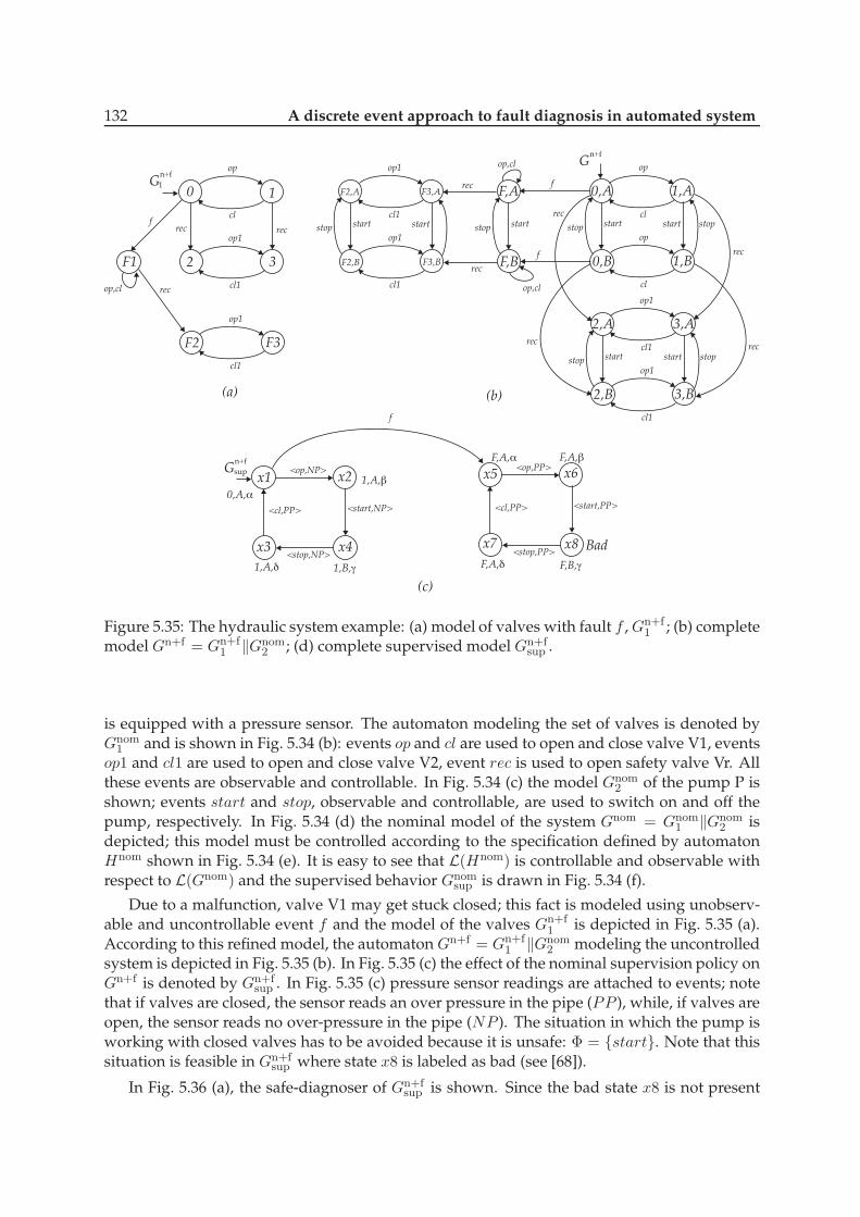
132 A discrete event approach to fault diagnosis in automated system
op
cl
op
cl
start
Gn+f
0,A 1,A
0,B 1,B
(c)
startstop stop
op1
cl1
op1
cl1
start
2,A 3,A
2,B 3,B
startstop stop
rec
rec
recrec
start
F,A
F,B
stop
f
f
rec
rec
op,cl
op,cl
(b)
<op,NP>
<cl,PP> <start,NP>
<stop,NP>
0,A,α
1,A,β
1,B,γ1,A,δ
Gn+f
sup <op,PP>
<cl,PP> <start,PP>
<stop,PP>
F,A,α F,A,β
F,B,γF,A,δ
x1 x2
x4x3
x5 x6
x8x7
f
Bad
op
cl
op1
cl1
rec recf
rec
Gn+f
1
op,cl
0 1
2 3F1
(a)
op1
cl1
F2 F3
op1
cl1
op1
cl1
start
F2,A F3,A
F2,B F3,B
startstop
Figure 5.35: The hydraulic system example: (a) model of valves with fault f , Gn+f1 ; (b) complete
model Gn+f = Gn+f1 ‖Gnom
2 ; (d) complete supervised model Gn+fsup .
is equipped with a pressure sensor. The automaton modeling the set of valves is denoted byGnom
1 and is shown in Fig. 5.34 (b): events op and cl are used to open and close valve V1, eventsop1 and cl1 are used to open and close valve V2, event rec is used to open safety valve Vr. Allthese events are observable and controllable. In Fig. 5.34 (c) the model Gnom
2 of the pump P isshown; events start and stop, observable and controllable, are used to switch on and off thepump, respectively. In Fig. 5.34 (d) the nominal model of the system Gnom = Gnom
1 ‖Gnom2 is
depicted; this model must be controlled according to the specification defined by automatonHnom shown in Fig. 5.34 (e). It is easy to see that L(Hnom) is controllable and observable withrespect to L(Gnom) and the supervised behavior Gnom
sup is drawn in Fig. 5.34 (f).
Due to a malfunction, valve V1 may get stuck closed; this fact is modeled using unobserv-able and uncontrollable event f and the model of the valves Gn+f
1 is depicted in Fig. 5.35 (a).According to this refined model, the automaton Gn+f = Gn+f
1 ‖Gnom2 modeling the uncontrolled
system is depicted in Fig. 5.35 (b). In Fig. 5.35 (c) the effect of the nominal supervision policy onGn+f is denoted by Gn+f
sup . In Fig. 5.35 (c) pressure sensor readings are attached to events; notethat if valves are closed, the sensor reads an over pressure in the pipe (PP ), while, if valves areopen, the sensor reads no over-pressure in the pipe (NP ). The situation in which the pump isworking with closed valves has to be avoided because it is unsafe: Φ = {start}. Note that thissituation is feasible in Gn+f
sup where state x8 is labeled as bad (see [68]).
In Fig. 5.36 (a), the safe-diagnoser of Gn+fsup is shown. Since the bad state x8 is not present
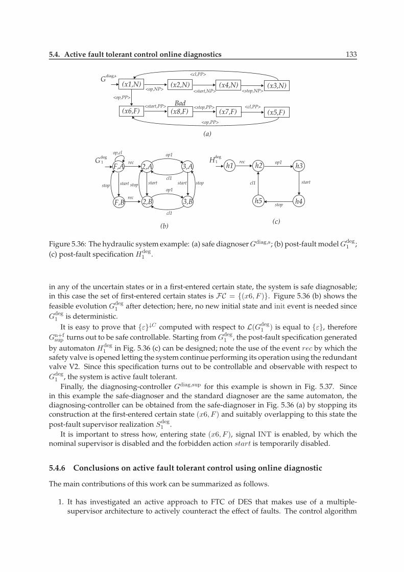
5.4. Active fault tolerant control online diagnostics 133
<op,NP>
<cl,PP>
<start,NP> <stop,NP>
Gdiag,s
<op,PP>
<cl,PP><start,PP> <stop,PP>
(x1,N) (x2,N) (x4,N) (x3,N)
(x6,F) (x8,F) (x7,F) (x5,F)
<op,PP>
Bad
(a)
(b)
op1
cl1
op1
cl1
start
2,A 3,A
2,B 3,B
startstop stop
recF,A
op,cl
(c)
op1
cl1 start
stop
rech1 h2 h3
h4h5
start
F,B
stop
rec
Gdeg
1 Hdeg
1
Figure 5.36: The hydraulic system example: (a) safe diagnoserGdiag,s; (b) post-fault modelGdeg1 ;
(c) post-fault specification Hdeg1 .
in any of the uncertain states or in a first-entered certain state, the system is safe diagnosable;in this case the set of first-entered certain states is FC = {(x6, F )}. Figure 5.36 (b) shows thefeasible evolution Gdeg
1 after detection; here, no new initial state and init event is needed sinceGdeg
1 is deterministic.It is easy to prove that {ε}↓C computed with respect to L(Gdeg
1 ) is equal to {ε}, thereforeGn+f
sup turns out to be safe controllable. Starting from Gdeg1 , the post-fault specification generated
by automaton Hdeg1 in Fig. 5.36 (c) can be designed; note the use of the event rec by which the
safety valve is opened letting the system continue performing its operation using the redundantvalve V2. Since this specification turns out to be controllable and observable with respect toGdeg
1 , the system is active fault tolerant.Finally, the diagnosing-controller Gdiag,sup for this example is shown in Fig. 5.37. Since
in this example the safe-diagnoser and the standard diagnoser are the same automaton, thediagnosing-controller can be obtained from the safe-diagnoser in Fig. 5.36 (a) by stopping itsconstruction at the first-entered certain state (x6, F ) and suitably overlapping to this state thepost-fault supervisor realization Sdeg
1 .It is important to stress how, entering state (x6, F ), signal INT is enabled, by which the
nominal supervisor is disabled and the forbidden action start is temporarily disabled.
5.4.6 Conclusions on active fault tolerant control using online diagnostic
The main contributions of this work can be summarized as follows.
1. It has investigated an active approach to FTC of DES that makes use of a multiple-supervisor architecture to actively counteract the effect of faults. The control algorithm

134 A discrete event approach to fault diagnosis in automated system
<op,NP>
<cl,PP>
<start,NP> <stop,NP>
Gdiag,sup
<op,PP>
(x1,N) (x2,N) (x4,N) (x3,N)
(x6,F) INT
op1
cl1 start
stop
rec
h2 h3
h4h5
Figure 5.37: The hydraulic system example: the diagnosing-controller Gdiag,sup.
employs online diagnosics to actively react to the detection of a malfunctioning compo-nent in order to eventually meet degraded control specifications.
2. It has evaluated the effect of the diagnostics algorithm on the FTC architecture, based onthe idea that “fast”fault-detection is needed to promptly react and reconfigure the systembefore it executes some unsafe action. To this aim, starting from an appropriate model ofthe system, we have shown how the notion of safe diagnosability is a necessary step inorder to achieve fault tolerant supervision of DES.
3. It has introduced the new notions of “safe controllability”and “active fault tolerant sys-tem”to characterize the conditions that must be satisfied when solving the FTC problemusing the active approach. Computational tests for these properties were presented.
4. It has proposed a procedure to design an automaton called “diagnosing-controller”which,embedding the diagnoser as well as the set of reconfigured controllers, is able, if the sys-tem satisfies the properties introduced, to solve the fault tolerant supervision problem.
Future research in this area could include the introduction of temporal behavior in the sys-tem model and the consideration of a decentralized/distributed FTC architecture. This lastpoint is of particular interest as it paves the way to the definition of meaningful reconfigura-tion strategies in which small faults are counteracted at the node level, whereas severe faultsare managed at a higher level involving a set of nodes.
Conclusions and future works
The main aim of this thesis, conclusive work of a three years research period focused on indus-trial automation software architectures, is the development of a design pattern for control logicin industrial automated systems. As explained in this work, in last years the industrial automa-tion processes have acquired an ever increasing degree of automation, this trend derives by thehigher requirement of systems in term of quality, productivity, efficiency. This increasing makecomplex the design of an industrial automated systems and in particular of its control system.This works starts with a survey chapter on automated industrial a systems, with a particu-lar mention to automated manufacturing systems, which illustrates the main characteristic ofthis system and some definition. Starting from this, and analyzing the state of the art of soft-ware engineering in industrial automation and the usually specification in an AMS we arrivedto define an architecture based on the new concept of the Generalized Device (GA). The mainconcept is the separation between the policy as a sequence of actions, and the actuation mech-anisms which perform the actions. This entity is defined in order to (i) encapsulate actuationmechanisms separating them from high level control policies in order to hierarchically managethe plant, (ii) support hardware virtualization, component interoperability and reusability and(iii) make easier the design of diagnostics, reconfiguration and quality check functionalities ex-ploiting a distributed and hierarchical approach. Inside the work some examples show howthis architecture has characteristic of modularity and composability. A lack in this approach isthe low reusability of the software, because is dependent from the particular hardware of theAMS. Starting from this point it was take under consideration this question “Do different fielddevices really need different control logic ?”In the GA approach an actuation mechanism was a set of an actuators and sensors to performan action. In AMS it is possible to find different devices from different fields (electric, pneu-matic, etc.) but analyzing the kind of signals that sensors and actuators need to exchange toperform an action, we can define a new entity called Generalize Device. In this way GD is “com-ponent”independent from the hardware, and so it is reusability. The main characteristic of thisarchitecture is the standardization of set of devices and a division of the diagnostic in two level:a low level and a high level diagnostic. The low level diagnostic is embedded inside the GDcomponent, in this level are presented algorithms of fault detection on sensors and actuatorsfaults (i.e. stuck low, stuck high) this kind of fault are independent from hardware and thespecific application of the AMS. High level faults means faults which are dependent from theapplication and to detect this faults it need use information generates from two or more de-vices.AMS are vulnerable systems so the diagnosis problem is an important topic. The faults isola-tion in a generic dynamical system consists in the design of an elaboration unit that, appropri-
135
136 Conclusions and future works
ately processing the inputs and outputs of the dynamical system, is also capable of detectingincipient faults on the plant devices, reconfiguring the control system so as to guarantee sat-isfactory performance. In the Gd component are embedded fault detection and fault isolationalgorithms but to guarantee the effectiveness of the diagnosis system, it should also keep intoaccount an appropriate plant model, that describes its behaviour starting from the knowledgeof some inputs and outputs. In the last part of this work, it was presented a general and ver-satile approach for building structured formal models in order to facilitate their control anddiagnosis using techniques from discrete events system theory. For this purpose, it was pre-sented a methodology for building in a modular manner the complete model of a complexautomated system starting from individual components and their physical coupling. Usingthis approach it is possible to have the faulty model of the entire system and using this havea formal proof that the fault detection algorithm are correct. Finally, also the topic of the faulttolerant control was explained.Future development of this work will be the study and the implementation of tools which areable to support the fulfillment of concepts of the Generalized Actuator and Generalized Device,in particular an important point should be a definition of formal methods for control code gen-eration to bridge the obtained results with the field of industrial informatics in order to obtain(semi)automatic code generation with respect to standard programming languages.Another very interesting research problem is the definition of a modeling framework able todescribe functionalities as well as the effect of their allocation and implementation over phys-ical resources. This modeling tool will be used to model architectures and components forcomputer-based distributed control systems with a clear distinction between functional andimplementative layer. This architecture should be modular and hierarchical in order to repre-sent, at different abstraction levels, the distributed nature of the system.All this effort will go in the direction to the definition of formal methods for the design andverification of the functional architecture; this point is devoted to the study of new supervisorycontrol architectures that, exploiting the distributed nature of the systems (decentralized con-trol, modular control etc.) and considering the effect of the integration with the implementationlayer, allow the compliance of key specifications such as safety and fault tolerance.

Appendixes
137


Appendix AIntroduction to discrete event systemstheory
In this appendix some notions about discrete event dynamical systems(DEDS) are reported, including basic definitions about discrete event sys-tems (DES), theory of automata and languages and some important re-sults about feedback supervision. The interested reader is referred fora more complete and formal treatment of these topics to [17], [98] andreferences therein.
A.1 Discrete event systems
A Discrete event system (DES) is a dynamical system in which the state space is naturally de-scribed by a discrete set, and the state transitions are only observed at discrete points in time.We associate the state transitions with “events”; an event can be identified with a specific actiontaken. This action can be spontaneous (dictated by nature) or it may be the result of several con-ditions which are suddenly met. The symbol e denotes an event; considering a system affectedby different types of events, we will assume we can define an event set E, whose elements areall these events.Discrete event systems satisfy the following two properties:
1. The state space is a discrete set.
2. The state transition mechanism is event drive.
Definition A.1 A discrete event system is a discrete-state, event-driven system, i.e. its state dependsentirely on the occurrence of asynchronous discrete events over time.
With this in mind, the behavior of a DES can be described in terms of event sequences of theform e1, e2, · · · , en. A more formal way to study the logical behavior of DES is based on thetheories of languages and automata.
139

140 Introduction to discrete event systems theory
The starting point is the fact that any DES has an underlying event set E associated withit. The set E is thought of as the alphabet of a language and event sequences are thought of asstrings (words) in that language. A string consisting of no events is called empty string and isdenoted by ǫ. The length of a string s, denoted with |s|, is the number of events contained in it,counting multiple occurrences of the same event.
Definition A.2 A language defined over a set E is a set of finite-length strings from events in E.
The key operation involved in building strings and thus languages from a set of events E isconcatenation: the string abb is the concatenation of the string ab and the event b. The emptystring ǫ is the identity element of concatenation. Let E⋆ denote the set of all finite stringsof elements of E, including the empty string ǫ; the (·)⋆ operation is called Kleene-closure. Alanguage over an event set E is a subset of E⋆.If tuv = s, the following nomenclature can be defined:
• t is called a prefix of s,
• u is called a substring of s,
• v is called a suffix of s.
Observe that both ǫ and s are prefixes, substrings and suffixes of s.
A.2 Operations on Languages
The usual set operations, such as union, intersection, difference and complement with respectto E⋆ are applicable to languages, since languages are sets. In addition it is possible to introducethe following operations:
• Concatenation: Let La, Lb ⊆ E⋆, then
LaLb := {s ∈ E⋆ : (s = sasb) and (sa ∈ La) and (sb ∈ Lb)} .
A string is in LaLb if it can be written as the concatenation of a string in La with a stringin Lb.
• Prefix-closure: Let L ⊆ E⋆, then
L := {s ∈ E⋆ : ∃t ∈ E⋆(st ∈ L)} .
The prefix closure of L is the language L consisting of all the prefixes of all the strings inL. In general L ⊆ L.
• Kleene-closure: Let L ⊆ E⋆, then:
L⋆ := {ǫ} ∪ L ∪ LL ∪ LLL ∪ · · · .
An element of L⋆ is formed by the concatenation of a finite number of elements of L.
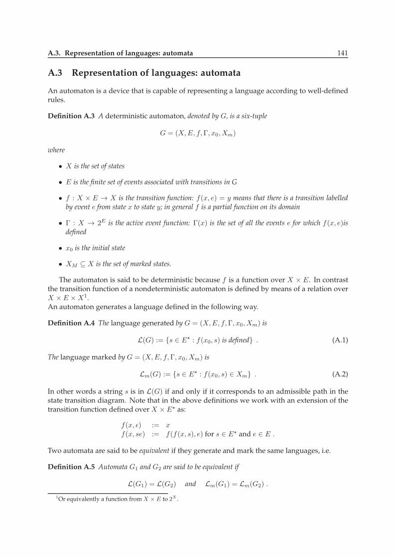
A.3. Representation of languages: automata 141
A.3 Representation of languages: automata
An automaton is a device that is capable of representing a language according to well-definedrules.
Definition A.3 A deterministic automaton, denoted by G, is a six-tuple
G = (X,E, f,Γ, x0,Xm)
where
• X is the set of states
• E is the finite set of events associated with transitions in G
• f : X × E → X is the transition function: f(x, e) = y means that there is a transition labelledby event e from state x to state y; in general f is a partial function on its domain
• Γ : X → 2E is the active event function: Γ(x) is the set of all the events e for which f(x, e)isdefined
• x0 is the initial state
• XM ⊆ X is the set of marked states.
The automaton is said to be deterministic because f is a function over X × E. In contrastthe transition function of a nondeterministic automaton is defined by means of a relation overX × E ×X1.An automaton generates a language defined in the following way.
Definition A.4 The language generated by G = (X,E, f,Γ, x0,Xm) is
L(G) := {s ∈ E⋆ : f(x0, s) is defined} . (A.1)
The language marked by G = (X,E, f,Γ, x0,Xm) is
Lm(G) := {s ∈ E⋆ : f(x0, s) ∈ Xm} . (A.2)
In other words a string s is in L(G) if and only if it corresponds to an admissible path in thestate transition diagram. Note that in the above definitions we work with an extension of thetransition function defined over X × E⋆ as:
f(x, ǫ) := xf(x, se) := f(f(x, s), e) for s ∈ E⋆ and e ∈ E .
Two automata are said to be equivalent if they generate and mark the same languages, i.e.
Definition A.5 Automata G1 and G2 are said to be equivalent if
L(G1) = L(G2) and Lm(G1) = Lm(G2) .
1Or equivalently a function from X × E to 2X .

142 Introduction to discrete event systems theory
In general the following property holds:
Lm(G) ⊆ L(G) ⊆ L(G) .
It can happen that an automaton G could reach a state x where Γ(x) = ∅, but x /∈ Xm. This issaid a deadlock, because no further event can be executed. If deadlock happens, then necessarilyLm(G) will be a proper subset of L(G), since any string in L(G) that ends at state x cannot be aprefix of a string in Lm(G).
Consider now the case when there is set of unmarked states in G that forms a stronglyconnected component, but with no transitions going out of the set. If the system enters this set,then we get a so-called livelock. If livelock is possible then again Lm(G) will be a proper subsetof L(G).
Definition A.6 An automaton G is said to be blocking if
Lm(G) ⊂ L(G)
and nonblocking when
Lm(G) = L(G) .
In other words if an automaton is blocking either deadlock and/or livelock can happen.Suppose now that an event e at state x may cause transitions to more than one state. In this
case f(x, e) is represented by a set of states. In addition we may want that to allow the label ǫ inthe state transition diagram, i.e. we allow transitions between distinct states to have the emptystring as label2. These two changes lead to the definition of a nondeterministic automaton.
Definition A.7 A nondeterministic automaton, denoted by Gnd, is a six-tuple
Gnd = (X,E ∪ {ǫ} , fnd,Γ, x0,Xm)
where
• fnd is a function fnd : X × E ∪ {ǫ} → 2X , that is fnd(x, e) ⊆ X whenever it is defined
• The initial state may be itself a set of states: x0 ⊆ X.
A.3.1 Operations on automata
• Accessible part: From the definition of L(G) and Lm(G), we can delete from G all statesthat are not accessible or reachable from x0 by some string in L(G) without affecting thelanguages generated and marked by G. When we delete a state we also delete all thetransitions that are attached to that state. We will denote this operation by Ac(G) (takingthe accessible part).
Ac(G) := (Xac, E, fac, x0,Xac,m)Xac := {x ∈ X : ∃s ∈ E⋆(f(x0, s) = x)}Xac,m := Xm ∩Xac
fac := f |Xac×E→Xac.
2These transitions may represent events that cause a change in the internal state but are not observable by anoutside observer.
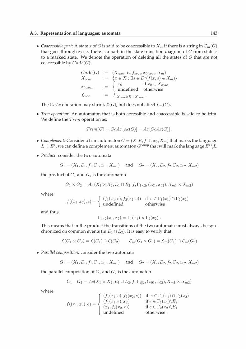
A.3. Representation of languages: automata 143
• Coaccessible part: A state x of G is said to be coaccessible to Xm if there is a string in Lm(G)that goes through x; i.e. there is a path in the state transition diagram of G from state xto a marked state. We denote the operation of deleting all the states of G that are notcoaccessible by CoAc(G):
CoAc(G) := (Xcoac, E, fcoac, x0,coac,Xm)Xcoac := {x ∈ X : ∃s ∈ E⋆(f(x, s) ∈ Xm)}
x0,coac :=
{
x0 if x0 ∈ Xcoac
undefined otherwisefcoac := f |Xcoac×E→Xcoac
.
The CoAc operation may shrink L(G), but does not affect Lm(G).
• Trim operation: An automaton that is both accessible and coaccessible is said to be trim.We define the Trim operation as:
Trim(G) = CoAc [Ac(G)] = Ac [CoAc(G)] .
• Complement: Consider a trim automaton G = (X,E, f,Γ, x0,Xm) that marks the languageL ⊆ E⋆, we can define a complement automaton Gcomp that will mark the language E⋆\L.
• Product: consider the two automata
G1 = (X1, E1, f1,Γ1, x01,Xm1) and G2 = (X2, E2, f2,Γ2, x02,Xm2)
the product of G1 and G2 is the automaton
G1 ×G2 = Ac (X1 ×X2, E1 ∩ E2, f,Γ1×2, (x01, x02),Xm1 ×Xm2)
where
f((x1, x2), e) =
{
(f1(x1, e), f2(x2, e)) if e ∈ Γ1(x1) ∩ Γ2(x2)undefined otherwise
and thusΓ1×2(x1, x2) = Γ1(x1)× Γ2(x2) .
This means that in the product the transitions of the two automata must always be syn-chronized on common events (in E1 ∩E2). It is easy to verify that:
L(G1 ×G2) = L(G1) ∩ L(G2) Lm(G1 ×G2) = Lm(G1) ∩ Lm(G2)
• Parallel composition: consider the two automata
G1 = (X1, E1, f1,Γ1, x01,Xm1) and G2 = (X2, E2, f2,Γ2, x02,Xm2)
the parallel composition of G1 and G2 is the automaton
G1 ‖ G2 = Ac(X1 ×X2, E1 ∪ E2, f,Γ1‖2, (x01, x02),Xm1 ×Xm2)
where
f((x1, x2), e) =
(f1(x1, e), f2(x2, e)) if e ∈ Γ1(x1) ∩ Γ2(x2)(f1(x1, e), x2) if e ∈ Γ1(x1)\E2
(x1, f2(x2, e)) if e ∈ Γ2(x2)\E1
undefined otherwise .

144 Introduction to discrete event systems theory
In the parallel composition a common event can only be executed if the two automataboth execute it simultaneously. The two automata are synchronized on common events.To characterized the language generated, we define the projection
Pi : (E1 ∪ E2)⋆ → E⋆
i for i = 1, 2
as follows:Pi(ε) = ǫ
Pi(e) =
{
e if e ∈ Ei
ǫ if e /∈ Ei
Pi(se) = Pi(s)Pi(e) for s ∈ (E1 ∪ E2)⋆, e ∈ (E1 ∪ E2).
In other words given two event sets where one is a subset of the other, this kind of pro-jection (called natural projection) erases events in a string formed from the larger set, thatdo not belong to the smaller one. We can also introduce the corresponding inverse maps(inverse projection)
P−1i : E⋆
i → 2(E1∪E2)⋆
defined as:P−1i = {s ∈ (E1 ∪ E2)
⋆ : Pi(s) = t} .
In other words given a string in the smaller event set, the inverse projection returns theset of all strings in the larger event set that project to the given string. The projectionsand their inverses are extended to languages, simply by applying them to all the stringsin the language. Note that
Pi
[
P−1i (L)
]
= L
but in generalL ⊆ P−1
i [Pi(L)] .
Returning to the parallel composition between automata, it easy now to prove that
L(G1 ‖ G2) = P−11 [L(G1)]∩P
−12 [L(G2)] Lm(G1 ‖ G2) = P−1
1 [Lm(G1)]∩P−12 [Lm(G2)] .
A.3.2 Observer automata
It is always possible transform a nondeterministic automaton Gnd into an equivalent deter-ministic one. We will call the resulting equivalent deterministic automaton the observer Gobs
corresponding to the nondeterministic automaton. The procedure to build the automaton canbe found in [17]. It is important just to recall the properties of the observer:
1. Gobs is a deterministic automaton.
2. L(Gobs) = L(Gnd)
3. Lm(Gobs) = Lm(Gnd)
We motivated previously the use of ǫ-transitions in a nondeterministic automaton as eventsthat occur in the system modelled by the automaton, but cannot be observed from outside.Those events are considered as unobservable events, in other words the event set is partitionedinto two disjoints parts:
E = Eo ∪ Euo

A.4. Regular languages 145
where Eo is the set of observable events and Euo is the set of unobservable events. Treatingunobservable events as ǫ-transitions and building the observer corresponding to the nondeter-ministic automaton obtained, it is easy to prove that the observer satisfy the following proper-ties:
• L(Gobs) = P [L(G)]
• Lm(Gobs) = P [Lm(G)]
• The state of Gobs that is reached after a string t ∈ P [L(G)] will contain all the states of Gthat can be reached after any strings in
P−1(t) ∩ L(G) .
Where P denotes the natural projection from E to Eo defined as follows:
P (ǫ) = ǫ
P (e) =
{
e if e ∈ Eo
ǫ if e /∈ Eo
P (se) = P (s)P (e) for s ∈ E⋆, e ∈ E.
In other words, the state of Gobs is the union of all the states of G that are consistent with theobservable events that have occurred so far. In this sense the state of Gobs is an estimate of thecurrent state of G.
A.4 Regular languages
Any language can be marked by an automaton: simply build the automaton as a possiblyinfinite tree whose root is the initial state and where the nodes at layer n of the tree are enteredbye the strings of length n or the prefixes of length n of the longer strings. The state space isthe set of nodes of the tree and a state is marked if and only if the string that reaches it fromthe root is an element of the language. Such tree automaton will have an infinite state spaceif the cardinality of the language is infinite. Of course there exist infinite languages that canbe represented by finite-state automaton3, but there exist also infinite languages that cannot berepresented by finite-state automata. A classical example is the language L = {anbn : n ≥ 0};see [17] for more details.
Definition A.8 A language is said to be regular if it can be marked by a finite-state automaton. Wewill denote the class of regular languages by R.
It is easy to prove the following theorems:
Theorem A.1 The class of languages representable by nondeterministic finite-state automata is exactlythe same as the class of languages representable by deterministic finite-state automata: R.
Theorem A.2 If L1 and L2 are in R, then the following languages are also in R:
1. L1
2. L⋆1
3The simplest case is the language L = E⋆ that can be represented by a single state automaton.

146 Introduction to discrete event systems theory
3. Lc := E⋆ \ L1
4. L1 ∪ L2
5. L1 ∩ L2
6. L1L2
Theorem A.3 A language is regular if and only if it can be represented by a regular expression i.e. bymeans of the operations of kleene-closure, union and concatenation.
A.5 Supervisory control
The situation considered in this section is that of a given DES whose behavior must be modifiedby feedback control in order to achieve a given set of specifications. Consider an automatonG that models the uncontrolled behavior of the DES; this behavior is not satisfactory and mustbe modified by control in the sense that its behavior must be restricted to a subset of L(G).In this framework, we consider sublanguages of L(G) that represent the legal behavior for thecontrolled system. In this paradigm, the supervisor S observes some of all the events that Gexecutes and tells G which events in its current active set are allowed next. In other words, Shas the capability of disabling some feasible events of G, exerting in this way a feedback controlaction on G.
Consider a DES modelled by the language generated L and the language marked Lm. Land Lm are defined over the event set E. Consider the case of a prefix-closed L. These twolanguages are generated and marked by an automaton
G = (X,E, f,Γ, x0,Xm) .
We want to design a supervisor S that interacts with G in a feedback manner as explainedpreviously. Let E be partitioned into two disjoint subsets:
E = Ec ∪ Euc
where
• Ec is the set of controllable events, i.e. those events that can be prevented from happening(disabled) by supervisor S;
• Euc is the set of uncontrollable events, i.e. those events that cannot be prevented fromhappening by supervisor S.
Assume for the moment that all the events in E executed by G are observed by S. A supervisorS is a function
S : L(G) → 2E
such that for each s ∈ L(G),S(s) ∩ Γ(f(x0, s))
is the set of enabled events that G can execute at its current state f(x0, s). In view of this we willsay that supervisor S is admissible if for all s ∈ L(G)
Euc ∩ Γ(f(x0, s)) ⊆ S(s)
i.e. S is not allowed to ever disable a feasible uncontrollable event.

A.5. Supervisory control 147
Definition A.9 The language generated by S/G is defined recursively as follows
1. ǫ ∈ L(S/G)
2. [(s ∈ L(S/G)) and (sσ ∈ L(G)) and (σ ∈ S(s))] ⇐⇒ [(sσ ∈ L(S/G))].
The language marked by S/G is defined as follows:
Lm(S/G) := L(S/G) ∩ Lm(G).
Definition A.10 The DES S/G is blocking if
L(S/G) 6= Lm(S/G)
and nonblocking ifL(S/G) = Lm(S/G).
Consider now the situation where the supervisor does not observe all the events that G exe-cutes, i.e. the event set E is partitioned into two disjoint subsets:
E = Eo ∪ Euo
where
• Eo is the set of observable events, i.e. those events that can be seen by supervisor S;
• Euo is the set of unobservable events, i.e. those events that cannot be seen by supervisor S.
In this case the feedback loop includes a natural projection P between G and the supervisor Sin the sense that the supervisor cannot distinguish between two strings s1 and s2 that have thesame projection and will issue the same control action: SP [P (s1)] = SP [P (s2)]. We define apartial-observation supervisor a function
SP : P [L(G)] → 2E .
This means that the control action can change only after the occurrence of an observable events,i.e. when P (s) changes.
Let us take the string t = t′σ (with σ ∈ Eo). SP (t) is the control action that applies toall strings in L(G) that belong to P−1(t′){σ} and to the unobservable continuations of thesestrings. However SP (t) may disable unobservable events and thus prevent some of these un-observable continuations. We define
Lt = P−1(t′){σ} (SP (t) ∩ Euo)⋆ ∩ L(G).
In words, Lt contains all the strings in L(G) that are subject to the control action SP (t). Nowremember that a supervisor is admissible if it does not disable uncontrollable events. HenceSP is admissible if for all t = t′σ ∈ P [L(G)],
Euc ∩
[
⋃
s∈Lt
Γ(f(x0, s))
]
⊆ SP (t).
Definition A.11 The language generated by SP /G is defined recursively as follows
1. ǫ ∈ L(SP /G)
2. [(s ∈ L(SP/G)) and (sσ ∈ L(G)) and (σ ∈ SP [P (s)])] ⇐⇒ [(sσ ∈ L(SP/G))].
The language marked by S/G is defined as follows:
Lm(SP /G) := L(SP/G) ∩ Lm(G) .

148 Introduction to discrete event systems theory
A.6 Uncontrollability problem
A.6.1 Dealing with uncontrollable events
In the following is presented the existence result for supervisors in presence of uncontrollableevents.
Theorem A.4 (Controllability theorem) Consider a DES G = (X,E, f,Γ, x0) where Euc ⊆ E isthe set of uncontrollable events. Let K ⊆ L(G), where K 6= ∅ is the admissible language. Then thereexists a supervisor S such that L(S/G) = K if and only if the controllability condition does hold, i.e.:
KEuc ∩ L(G) ⊆ K .
Proof. See [17]. ⊳
Remark A.1 The controllability condition in controllability theorem is intuitive and can be paraphrasedas: “if you cannot prevent it, then it should be legal”.
Definition A.12 (controllability) Let K and M = M be languages over set E. Let Euc be a subsetof E. K is said to be controllable with respect to M and Euc if and only if
KEuc ∩M ⊆ K .
Theorem A.5 (Nonblocking Controllability theorem) Consider the DES G = (X,E, f,Γ, x0)where Euc ⊆ E is the set of uncontrollable events. Consider the language K ⊆ Lm(G), where K 6= ∅ isthe admissible language. Then there exists a nonblocking supervisor S for G such that Lm(S/G) = Kand L(S/G) = K if and only if:
1. K is controllable with respect to L(G) and Euc, i.e.:
KEuc ∩ L(G) ⊆ K ,
2. K is Lm(G)-closed, i.e.K = K ∩ Lm(G) .
Proof. See [17]. ⊳
A.6.2 Realization of supervisors
Let us assume that language K ⊆ L(G) is controllable, then from controllability theorem weknow that supervisor S defined by
S(s) = [Euc ∩ Γ(f(x0, s))] ∪{
σ ∈ Ec : sσ ∈ K}
results inL(S/G) = K .
We need now to build a convenient representation of the function S. Consider now an automa-ton R that marks the language K :
R = (Y,E, g,ΓR, y0, Y )

A.7. Unobservability problem 149
where R is trim andLm(R) = L(R) = K.
If we connect R to G by the product operation, the result R×G is exactly the behavior we desirefor S/G:
L(R×G) = L(R) ∩ L(G)
= K ∩ L(G)
= K = L(S/G)
Lm(R×G) = Lm(R) ∩ Lm(G)
= K ∩ Lm(G)
= L(S/G) ∩ Lm(G) = L(S/G) .
Note that R is defined to have the same event set as G, then R ‖ G = R×G. We will call R thestandard realization of S.
A.7 Unobservability problem
Consider now the feedback loop in the case of partial event observation. In other words wehave to deal with the presence of unobservable events in addition to the presence of uncon-trollable events. Clearly unobservable events impose further limitations on the controlled be-haviors that can be achieved with P -supervisors. As we did for controllability, we need tointroduce the concept of observability. Intuitively observability means “if you cannot differentiatebetween two strings, then these strings should require the same control action”, or equivalently “if youmust disable an event after observing a string, then by doing so you should not disable any string thatappears in the desired behavior”. This idea can be formalized as follows:
Definition A.13 (observability) Let K and M = M be languages over set E. Let Ec be a subset ofE. Let Eo be another subset of E with P as the corresponding natural projection from E⋆ to E⋆
o . K issaid to be observable with respect to M , P and Ec if for all s ∈ K and for all σ ∈ Ec,
(sσ /∈ K) and (sσ ∈ M) ⇒ P−1 [P (s)] σ ∩K = ∅ .
Theorem A.6 (Controllability and observability theorem) Consider DES G = (X,E, f,Γ, x0)where Euc ⊆ E is the set of uncontrollable events and Eo ⊆ E is the set of observable events. Let Pbe the natural projection from E⋆ to E⋆
o . Consider the language K ⊆ Lm(G), where K 6= ∅ is theadmissible language. Then there exists a nonblocking P-supervisor SP for G such that Lm(SP/G) = Kand L(SP /G) = K if and only if:
1. K is controllable with respect to L(G) and Euc.
2. K is observable with respect to L(G), P and Euc.
3. K is Lm(G)-closed.
Proof. See [17]. ⊳
The reader interested in further results regarding supervision of uncontrollable and unob-servable languages is referred to [17] and references therein.

150 Introduction to discrete event systems theory
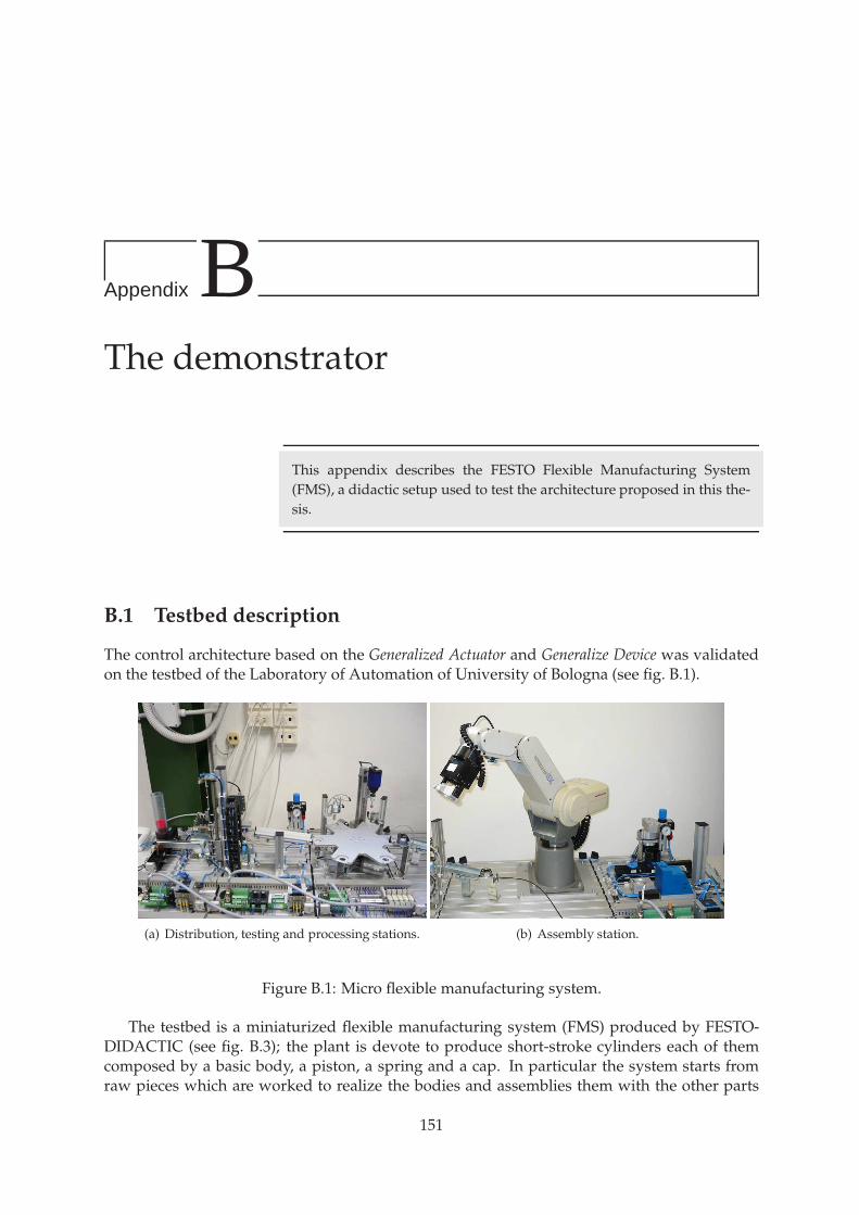
Appendix BThe demonstrator
This appendix describes the FESTO Flexible Manufacturing System(FMS), a didactic setup used to test the architecture proposed in this the-sis.
B.1 Testbed description
The control architecture based on the Generalized Actuator and Generalize Device was validatedon the testbed of the Laboratory of Automation of University of Bologna (see fig. B.1).
(a) Distribution, testing and processing stations. (b) Assembly station.
Figure B.1: Micro flexible manufacturing system.
The testbed is a miniaturized flexible manufacturing system (FMS) produced by FESTO-DIDACTIC (see fig. B.3); the plant is devote to produce short-stroke cylinders each of themcomposed by a basic body, a piston, a spring and a cap. In particular the system starts fromraw pieces which are worked to realize the bodies and assemblies them with the other parts
151

152 The demonstrator
CAP
SPRING
PISTON
BASIC BODY
(a) Short-stroke cylin-ders.
(b) PLC.
Figure B.2: Control hardware and short-stroke cylinders.
to obtain the desired cylinder (see fig. B.2(a)). Thanks to the use of different basic bodies itis possible to realize different diameter cylinders. In the following cylinders’ bodies will bereferred as workpieces.
The FMS is composed by four stations (see fig. B.3): the first station is the distributionstation, where the workpiece is picked from the raw materials warehouse and moved to thesecond station, the testing station. In testing station the workpiece is measured and its colorand height is identified. According to this measurements the workpiece is discarded or movedto the processing station; in this station the workpiece is tested to verify if it can be worked ornot. If the workpiece positively passes the test, it is drilled and then moved to the last station,the assembly station, where workpieces are assembled by a robotic manipulator to realize thecylinder. The control of the FMS is implemented on a ABB PLC, AC500 family equipped withCPU PM581-ETH with four input/output modules DC523 (see fig. B.2(b)).Exhaustive informations on the FESTO FMS can be find in [33], [35], [34] and [32]. The controlsoftware has been developed using the software suite CoDeSys (Controller Development Sys-tem) [2], a CACSD tool that allows a completely IEC 61131-3 compliance. For more informationon the Laboratory of Automation of University of Bologna see [18].
B.1.1 Distribution station
The distribution station (see fig. B.4) fetches the bases of cylinders from an apposite warehouseand moves them to the testing station with the aid of a rotary arm. This station is composed bythe following devices:
• Raw pieces warehouse: is a FIFO warehouse with the maximum capability of eightpieces: a fiber optic presence sensor furnish an high logic level signal when there areno pieces in the warehouse.
• Extraction cylinder: is a single acting pneumatic cylinder whose function is to extract aload from the warehouse. The device is equipped with two inductive sensors sensible tothe magnetic field of the piston head. These two limit switch sensors indicates the endpositions of the cylinder.

B.1. Testbed description 153
����
Testing station
Distribution station
Assembly station
Processing station
Figure B.3: Micro flexible manufacturing system.
• Rotary arm: is a pneumatic rotary manipulator whose movement amplitude can be con-trolled by mechanical stops. The rotary arm transfers the raw pieces extracted from ware-house to the testing station. The arm is a double acting pneumatic device and its extremepositions are signaled by two electric microswitch activated directly by the arm. To an ex-tremity of the rotary arm there is a suction cup necessary to the capture of the raw piecesby the device. A vacuum sensor indicates when the load is correctly captured.
The usually sequence of operations are:
1. The rotary drive swivels to the position “downstream station” if workpieces are identifiedin the magazine and the START button is pressed.
2. The ejecting cylinder retracts and pushes a workpieces out of the magazine.
3. The rotary drive swivels to the position “magazine”.
4. The vacuum is switched on. When the workpiece is securely held, a vacuum switchswitches.
5. The ejecting cylinder advances and releases the workpiece.
6. The rotary drive swivels to the position “downstream station”.
7. The vacuum is switched off.

154 The demonstrator
Raw pieces warehouse: Rotary arm
Extraction cylinder
Figure B.4: Distribution Station layout
Signals Meaning when active Type
EMPTYWAREHOUSE warehouse is empty IN
CYLINDEREXTRACTSLOADFROMWAREHOUSE extract workpiece from warehouse OUT
CYLINDEREXTRACTIONLOADINEXTENSIVEPOSITION extraction link extended position IN
CYLINDEREXTRACTIONLOADINRETROACTIVEPOSITION extraction link retracted position IN
LIGHTEMPTYWAREHOUSE empty warehouse alarm OUT
ROTARYMAKERVSWAREHOUSE Rotary link moving to warehouse OUT
ROTARYMAKERVSVERIFICATION Rotary link moving to verification station OUT
ROTARYMAKERINPOSITIONWAREHOUSE Rotary link reaches warehouse IN
ROTARYMAKERINPOSITIONVERIFICATION Rotary link reaches verification station IN
VACUUMGENERATOR Vacuum generation OUT
VACUUMGENERATOROK Vacuum generator grasp workpiece IN
EXPULSIONAIRVACUUM Expelled workpiece from vacuum generator OUT
Table B.1: List of signals used in distribution station.
8. The rotary drive swivels to the position “magazine”.
B.1.2 Testing station
The testing station (see fig. B.5) is devoted to checks the colour and the height of a base and,according to the user requests (by the control panel), it decides to send or not the base to theprocessing station. This station is composed by the following devices.
• Testing module: its purpose is to recognize the kind of raw pieces. It includes a capacitivesensor that furnish an high level logic signal if a load is present and a colour sensor to

B.1. Testbed description 155
Testing module
Measurament module
Lifting module
Ejecting cylinder
Figure B.5: Testing station layout
sense the colour of the piece. This is a diffuse light sensor which generate an infraredradiation and change it’s state when this radiation returns to the sensor meaning that theload present in the testing station is not black.
• Lifting module: depending by the raw pieces colour and by the user’s specification, themodule must lift the raw pieces to the measurement module or stay in the low position toallow the piece expulsion. It is a rodless linear pneumatic drive utilizing magnetic forcetransmission without mechanical connection. Two inductive sensor are used to indicatethe ends position of the lifting module. A retro-reflective sensor is used to sense thepresence of the rotary arm into the trajectory of the lifting module in order to avoid amechanical interference. A single acting pneumatic cylinder mounted on the elevatorplatform perform the expulsion of the load from the testing station, an inductive sensorindicates its retract end-position. The expulsion of the load toward the processing stationis possible thanks to an air guide that reduce the friction of the load along the exit ramp.
• Measurement module: the purpose of this module is to recognize the height of the rawpieces presents in the station. This measurement must respects that of colour otherwisethe piece cannot proceed to the processing station and must be removed from the produc-tive line. This module consists of an analogue displacement sensor that is a conductiveplastic potentiometer which furnish, as output, an analogue voltage which is sent to aanalogue comparator. The comparator has three digital output which are at high logiclevel depending by the value of two threshold voltage set by the user. In this way it’spossible to have a digital signal that inform on the presence of a Red/Silver (which havethe same height) piece or Black piece.

156 The demonstrator
Signal Meaning when active Type
READYLOADFORVERIFICATION Workpiece in verification station IN
COLOURMEASUREMENT Red or silver workpiece IN
TOLIFTCYLINDERTOMEASURELOAD Move the lift upward OUT
TOLOWERCYLINDERTOMEASURELOAD Move the lift downward OUT
CYLINDERUPTOMEASURELOAD The lift is in upward position IN
CYLINDERDOWNTOMEASURELOAD The lift is in upward position IN
TOEXTENDCYLINDEROFEXTRACTIONVSGUIDE Extraction cylinder expel a workpiece OUT
CYLINDEROFEXTRACTIONINRETROACTIVEPOSITION Extraction cylinder in retractive position IN
AIRCUSHION Activate air cushion OUT
MEASUREMENTNOTOK Bad workpiece IN
Table B.2: List of signals used in testing station.
The usually sequence of operations are:
1. Determine the colour and material of the workpiece.
2. Lifting cylinder to be raised.
3. Measurement of the workpiece height
If testing result is OK the sequence of operation are:
1. Switch on the air cushioned slide.
2. Ejecting cylinder to advance.
3. Ejecting cylinder to retract.
4. Switch off the air cushioned slide.
5. Lifting cylinder to be lowered.
6. Initial position.
If testing result is not OK the usually sequence of operation are:
1. Lifting cylinder to be lowered.
2. Ejecting cylinder to be advanced.
3. Ejecting cylinder to retract.
4. Initial position.
B.1.3 Processing Station
The processing station (see fig. B.6) function is to perform a processing simulation on the rawpieces: a rotary table is used to move the raw pieces into three different working module. Firstthe piece is tested to verify if it can be worked or not: a raw piece can be worked only if it iscorrect oriented. If the base successfully passes the test, it is drilled to create the hole for thespring and the piston. After this operation the load is moved toward the expelling module forbeing transfered at the assembly station. This station is only electrically actuated; no pneumaticdevices are present.
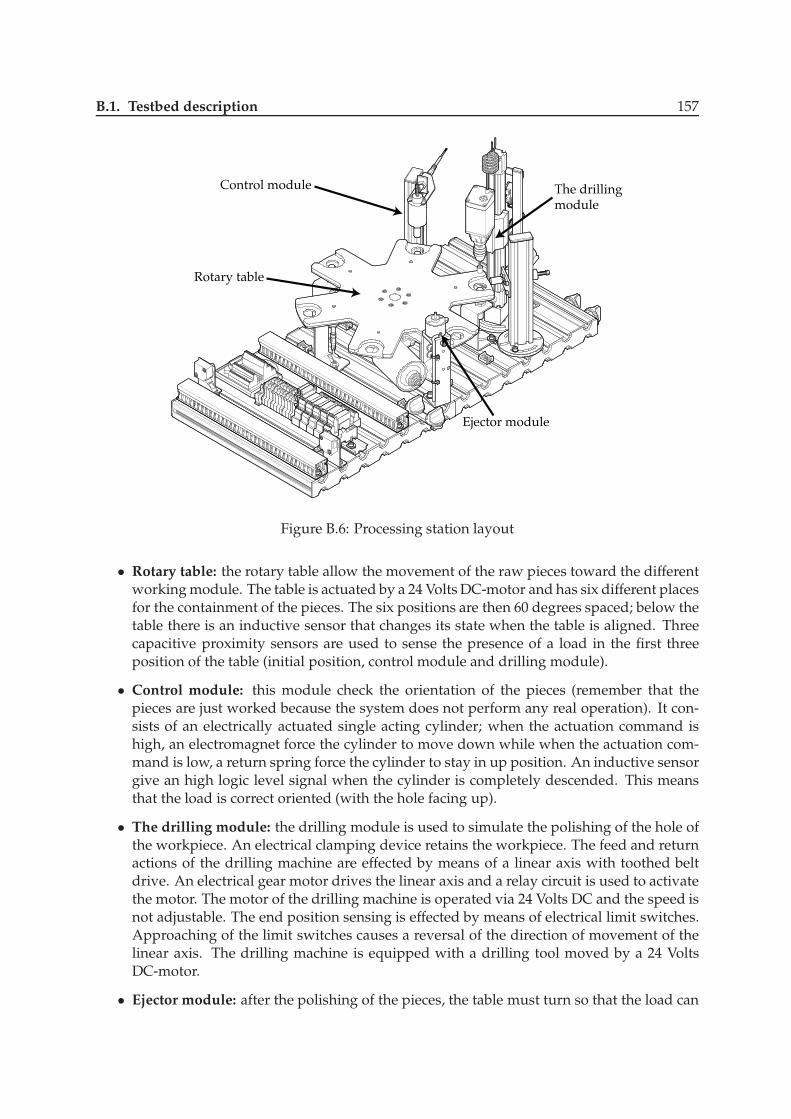
B.1. Testbed description 157
Rotary table
Control module The drillingmodule
Ejector module
Figure B.6: Processing station layout
• Rotary table: the rotary table allow the movement of the raw pieces toward the differentworking module. The table is actuated by a 24 Volts DC-motor and has six different placesfor the containment of the pieces. The six positions are then 60 degrees spaced; below thetable there is an inductive sensor that changes its state when the table is aligned. Threecapacitive proximity sensors are used to sense the presence of a load in the first threeposition of the table (initial position, control module and drilling module).
• Control module: this module check the orientation of the pieces (remember that thepieces are just worked because the system does not perform any real operation). It con-sists of an electrically actuated single acting cylinder; when the actuation command ishigh, an electromagnet force the cylinder to move down while when the actuation com-mand is low, a return spring force the cylinder to stay in up position. An inductive sensorgive an high logic level signal when the cylinder is completely descended. This meansthat the load is correct oriented (with the hole facing up).
• The drilling module: the drilling module is used to simulate the polishing of the hole ofthe workpiece. An electrical clamping device retains the workpiece. The feed and returnactions of the drilling machine are effected by means of a linear axis with toothed beltdrive. An electrical gear motor drives the linear axis and a relay circuit is used to activatethe motor. The motor of the drilling machine is operated via 24 Volts DC and the speed isnot adjustable. The end position sensing is effected by means of electrical limit switches.Approaching of the limit switches causes a reversal of the direction of movement of thelinear axis. The drilling machine is equipped with a drilling tool moved by a 24 VoltsDC-motor.
• Ejector module: after the polishing of the pieces, the table must turn so that the load can

158 The demonstrator
Signal Meaning when active Type
ALIGNEMENTROTARYTABLEWITHPOSITIONING Rotary table is aligned IN
ROTARYTABLEMOTOR Move the rotary table OUT
INCONTROLLOADINWRONGPOSITIONTOBEDRILLED The workpiece is upside-down IN
AVAILABLELOADINCONTROLPOSITIONING The workpiece is in the testing module IN
TOLOWERCYLINDERTOINSPECTLOAD Test the workpiece in testing unit OUT
AVAILABLELOADINDRILLINGPOSITIONING The workpiece is in the drilling module IN
BLOCKINGCYLINDERFORWARDINDRILLINGPOSITIONING Lock the workpiece in the drilling module OUT
DRILLINGUNITDOWN Drilling machine has reached the downward limit IN
DRILLINGUNITUP Drilling machine has reached the upward limit IN
TOLOWERDRILLINGUNIT Move downward the drilling machine OUT
TOLIFTDRILLINGUNIT Move upward the drilling machine OUT
DRILLINGUNITCLOCKWISE Select clockwise rotation OUT
DRILLINGUNITUNCLOCKWISE Select counter-clockwise rotation OUT
DRILLINGUNITACTIVE Activate rotation of drilling machine OUT
EXPELLINGLEVERACTIVE Expel the workpiece in pushing-out module OUT
LIGHTUPSIDEDOWNLOADINEXPELLING Activate alarm of upside-down workpiece OUT
Table B.3: List of signals used in processing station.
be sent into the assembly station by the ejector module. The module is an electricallyactuated lever; when the actuation command is high the lever expels the load while re-moving the command the lever returns on its initial position. As mentione before, in thisposition there is no a presence sensor for the load.
The usually sequence of operations are:
1. The rotary indexing table is rotated by 60◦, if a workpiece is detected in the workpieceretainer 1 and the START pushbutton is pressed.
2. The solenoid plunger moves downwards and checks whether the workpiece is insertedwith the opening facing upwards. The rotary indexing table is rotated by 60¡ if the resultof the check is OK.
3. The clamping device clamps the workpiece. The motor of the drilling machine is switchedon. The linear axis moves the drilling machine downwards.
4. When the drilling machine has reached its lower position, it is moved to its upper stopagain by the linear axis.
5. The motor of the drilling machine is switched off and the clamping device is retracted.The rotary indexing table is rotated by 60◦.
6. The electrical sorting gate passes on the workpiece to a subsequent station.
B.1.4 Assembly station
This station (see fig. B.7) supplies the components of the cylinder for the assembly process. Theassembly is performed by a five degrees of freedom manipulator.
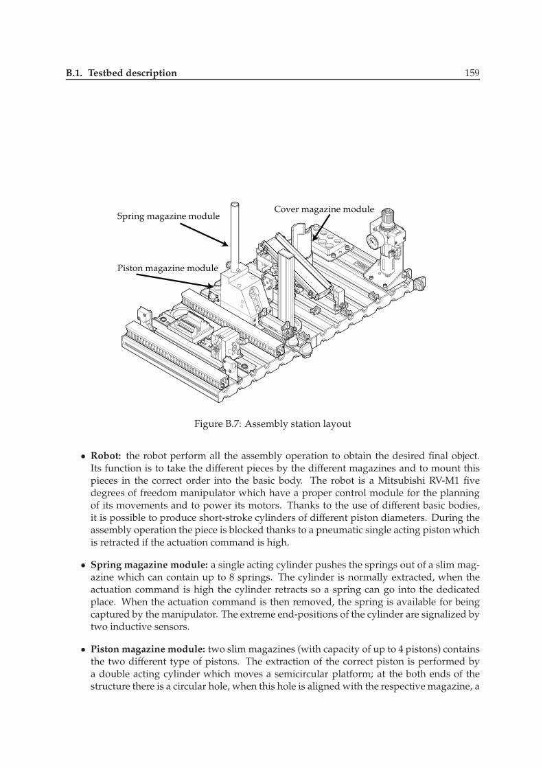
B.1. Testbed description 159
Spring magazine module
Piston magazine module
Cover magazine module
Figure B.7: Assembly station layout
• Robot: the robot perform all the assembly operation to obtain the desired final object.Its function is to take the different pieces by the different magazines and to mount thispieces in the correct order into the basic body. The robot is a Mitsubishi RV-M1 fivedegrees of freedom manipulator which have a proper control module for the planningof its movements and to power its motors. Thanks to the use of different basic bodies,it is possible to produce short-stroke cylinders of different piston diameters. During theassembly operation the piece is blocked thanks to a pneumatic single acting piston whichis retracted if the actuation command is high.
• Spring magazine module: a single acting cylinder pushes the springs out of a slim mag-azine which can contain up to 8 springs. The cylinder is normally extracted, when theactuation command is high the cylinder retracts so a spring can go into the dedicatedplace. When the actuation command is then removed, the spring is available for beingcaptured by the manipulator. The extreme end-positions of the cylinder are signalized bytwo inductive sensors.
• Piston magazine module: two slim magazines (with capacity of up to 4 pistons) containsthe two different type of pistons. The extraction of the correct piston is performed bya double acting cylinder which moves a semicircular platform; at the both ends of thestructure there is a circular hole, when this hole is aligned with the respective magazine, a
160 The demonstrator
piston from the warehouse falls into the hole. This piston can be expelled by a subsequentrotation of the platform. The extreme end-positions of the platform are indicated by twoinductive sensors.
• Cover magazine module: a single acting cylinder pushes the springs out of the covermagazine which can contain up to 8 covers. The device is equipped with two inductivesensors which indicates the end positions of the cylinder. A fiber optic presence sensorfurnish an high logic signal when there are no covers in the warehouse.
The usually sequence of operation are:
1. If a workpiece “body” is detected in the retainer and the START pushbutton at the robotcontroller is actuated the body is picked up by the robot.
2. The body is transported to the Assembly retainer module and placed at the “change grip-per” position.
3. The colour of the body is determined.
4. The body is picked up and the orientation is checked.
If there is a black workpiece the operation are:
1. The body is placed in the correct orientation in the “assembly” position.
2. A metallic piston is picked up at the pallet. The piston is inserted in the body.
3. The robot checks whether a spring is available. If it is, the spring is picked up and placedon the piston.
4. The robot checks whether a cap is available. If it is, the cap is picked up and placed onthe bolt of the Assembly retainer module. The orientation of the cap is checked.
5. The cap is placed in the correct orientation on the body. The cap is fixed by means ofrotation.
6. The finished pneumatic cylinder is placed on the slide.
If there is a red or silver workpiece the operation are:
1. The body is placed in the correct orientation in the “assembly” position.
2. A black piston is picked up at the pallet. The piston is inserted in the body.
3. The robot checks whether a spring is available or not. If it is, the spring is picked up andplaced on the piston.
4. The robot checks whether a cap is available or not. If it is, the cap is picked up and placedon the bolt of the Assembly retainer module. The orientation of the cap is checked.
5. The cap is placed in the correct orientation on the body. The cap is fixed by means ofrotation.
6. The finished pneumatic cylinder is placed on the slide.

B.2. Part of code of FESTO 161
Signal Meaning when active Type
TOEXTRACTSPRINGINASSEMBLYSTATION Spring extraction OUT
TOEXTRACTSPRINGINASSEMBLYSTATIONINEXTENSIVEPOSITION Spring extraction link extended IN
TOEXTRACTSPRINGINASSEMBLYSTATIONINRETROACTIVEPOSITION Spring extraction link retroactive IN
PISTONSELECTORGOONTHERIGHT Piston warehouse rotates to the right OUT
PISTONSELECTORGOONTHELEFT Piston warehouse rotates to the left OUT
PISTONSELECTORISONTHERIGHT Piston warehouse in right position IN
PISTONSELECTORISONTHELEFT Piston warehouse in left position IN
TOEXTRACTCOVERINASSEMBLYSTATIONFORWARD Cap extraction from warehouse OUT
TOEXTRACTCOVERINASSEMBLYSTATIONINRETROACTIVEPOSITION Link cap extraction in retroactive position IN
TOEXTRACTCOVERINASSEMBLYSTATIONINEXTENSIVEPOSITION Link cap extraction in extensive position IN
EMPTYCOVERHOUSEINASSEMBLYSTATION Cap warehouse is empty IN
BLOCKINGCYLINDERFORWARDINASSEMBLYSTATION Unlock workpiece OUT
ROBOTINPISTONWAREHOSE Robot in piston warehouse position IN
ROBOTINSPRINGWAREHOUSE Robot in spring warehouse position IN
ROBOTINCOVERWAREHOUSE Robot in cap warehouse position IN
ROBOTINASSEMBLYUNIT Robot in assembly position IN
ROBOTTAKECURRENTLOADTOASSEMBLYINASSEMBLYUNIT Workpiece assembly OUT
ROBOTGOTOPISTONHOUSE Robot grasp piston OUT
ROBOTGOTOSPRINGHOUSE Robot grasp spring OUT
ROBOTGOTOCOVERHOUSE Robot grasp cap OUT
ROBOTGOTOINITIALHOUSE Robot move in initial position OUT
Table B.4: List of signals used in assembly station.
B.2 Part of code of FESTO
In figure B.8 and figure B.9 are reported a little part of code of FESTO with GA approach. Fol-lowing is reported the code of the GD:
CASE GD_Init OF1: IF Activated THEN
DeviceState:=DeviceActivated;END_IF;IF Deactivated THEN
DeviceState:=DeviceDeactivated;END_IF;IF (NOT Activated AND NOT Deactivated) THEN
DeviceState:=DeviceStopped;END_IF;
0: CASE DeviceState OF
DeviceDeactivated:DeactivationRequest:=FALSE;IF (ActivationRequest) THEN
Activation:=TRUE;
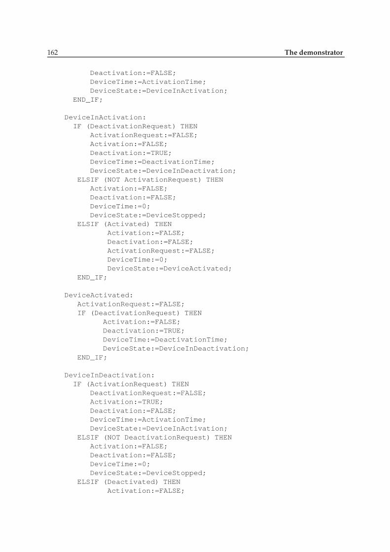
162 The demonstrator
Deactivation:=FALSE;DeviceTime:=ActivationTime;DeviceState:=DeviceInActivation;
END_IF;
DeviceInActivation:IF (DeactivationRequest) THEN
ActivationRequest:=FALSE;Activation:=FALSE;Deactivation:=TRUE;DeviceTime:=DeactivationTime;DeviceState:=DeviceInDeactivation;
ELSIF (NOT ActivationRequest) THENActivation:=FALSE;Deactivation:=FALSE;DeviceTime:=0;DeviceState:=DeviceStopped;
ELSIF (Activated) THENActivation:=FALSE;Deactivation:=FALSE;ActivationRequest:=FALSE;DeviceTime:=0;DeviceState:=DeviceActivated;
END_IF;
DeviceActivated:ActivationRequest:=FALSE;IF (DeactivationRequest) THEN
Activation:=FALSE;Deactivation:=TRUE;DeviceTime:=DeactivationTime;DeviceState:=DeviceInDeactivation;
END_IF;
DeviceInDeactivation:IF (ActivationRequest) THEN
DeactivationRequest:=FALSE;Activation:=TRUE;Deactivation:=FALSE;DeviceTime:=ActivationTime;DeviceState:=DeviceInActivation;
ELSIF (NOT DeactivationRequest) THENActivation:=FALSE;Deactivation:=FALSE;DeviceTime:=0;DeviceState:=DeviceStopped;
ELSIF (Deactivated) THENActivation:=FALSE;

B.2. Part of code of FESTO 163
Deactivation:=FALSE;DeactivationRequest:=FALSE;DeviceTime:=0;DeviceState:=DeviceDeactivated;
END_IF;
DeviceStopped:IF (ActivationRequest AND NOT DeactivationRequest) THEN
Activation:=TRUE;Deactivation:=FALSE;DeviceTime:=ActivationTime;DeviceState:=DeviceInActivation;
END_IF;IF (DeactivationRequest AND NOT ActivationRequest) THEN
Activation:=FALSE;Deactivation:=TRUE;DeviceTime:=DeactivationTime;DeviceState:=DeviceInDeactivation;
END_IF;
END_CASE;END_CASE;(*Gestione Temporizzazione GD*)IF (ClockT AND (DeviceTime>0)) THEN
DeviceTime:=DeviceTime-1;END_IF;Timeout:=(DeviceTime=0);(****SEGNALAZIONI DIAGNOSTICA***)FaultSensorDeviceActivated:=((DeviceState=DeviceDeactivatedAND Deactivated AND Activated) OR(Activation AND NOT Deactivation AND NOT Deactivated AND NOT Activated)OR (DeviceState=DeviceActivated AND NOT Deactivated AND NOT Activated))AND Timeout;FaultSensorDeviceDeactivated:=((DeviceState=DeviceDeactivated AND
NOT Deactivated AND NOT Activated) OR(NOT Activation AND Deactivation AND NOT Deactivated AND NOT Activated)OR (DeviceState=DeviceActivated AND Deactivated AND Activated))AND Timeout;
FaultActuator:=((DeviceState=DeviceDeactivated AND (NOT DeactivatedAND Activated)) OR (DeviceState=DeviceActivated AND(Deactivated AND NOT Activated)) OR(Activation AND NOT Deactivation AND Deactivated AND NOT Activated) OR(NOT Activation AND Deactivation AND NOT Deactivated AND Activated))AND Timeout;
DeviceFault:= FaultSensorDeviceActivated ORFaultSensorDeviceDeactivated OR FaultActuator;

164 The demonstrator
DoneWhat:=’EndInit’;END_IF;
Init3: IF (NOT DO_) THEN ( * Resetto il DONE quando la politica resetta il DO * )StateGaExtractionCylinderST:=Ready;State:=’Ready’;StateInit:=Init1;Done:=FALSE;
END_IF;END_CASE;
Ready: IF (DO_) THEN ( * Aspetto il comando di inizio operazionidalla politica * )
StateGaExtractionCylinderST:=Busy;StateBusy:=Busy1;State:=’Busy’;
END_IF;
( * In Busy ho 5 sottostati Busy1 (Controllo tipo di comando ’do’ e loeseguo) * )Busy: CASE StateBusy OF
Busy1: IF (DoWhat=’ExtractionCylinderOut’) AND SensorEmptyWarehouse = FALSE THEN ( * estraggo un pezzo dal magazzino * )CommandCylinderExtractsLoadFromWarehouse:=TRUE;StateBusy:=Busy2;
END_IF;IF (DoWhat=’ExtractionCylinderIn’) THEN ( * disattivo l’attuatore per far tornare ilcilindro di estrazione in posizione retratta * )
CommandCylinderExtractsLoadFromWarehouse:=FALSE;StateBusy:=Busy3;
END_IF;IF (DoWhat=’ExtractionCylinderOut’) AND SensorEmptyWarehouse = TRUE THEN ( * accendo laluce magazzino vuoto * )
CommandLightEmptyWarehouse:=TRUE;Done:=TRUE;DoneWhat:=’None’;StateBusy:=Busy4;
END_IF;IF (DoWhat=’ControlLoadPresence’) THEN ( * accendo la lucemagazzino vuoto * )
CommandLightEmptyWarehouse:=TRUE;StateBusy:=Busy5;
END_IF;
Busy2: IF SensorCylinderExtractionLoadInExtensivePosition =TRUE THEN ( * Busy2: aspetto cheil cilindro di estrazione sia in posizione estesa * )
StateBusy:=Busy4;CommandCylinderExtractsLoadFromWarehouse:=TRUE;Done:=TRUE;DoneWhat:=’ExtractionCylinderOut’;
END_IF;
Busy3: IF SensorCylinderExtractionLoadInRetroactivePosition = TRUE THEN ( * Busy3: aspetto cheil cilindro di estrazione sia in posizione retratta * )
StateBusy:=Busy4;CommandCylinderExtractsLoadFromWarehouse:=FALSE;DoneWhat:=’ExtractionCylinderIn’;Done:=TRUE;
END_IF;
Busy4: IF (NOT DO_) THEN ( * Busy4: �ne operazioni GA * )Done:=FALSE;StateGaExtractionCylinderST:=Ready;State:=’Ready’;StateBusy:=Busy1;
END_IF;
Busy5: IF PushButtonFullWarehouse = TRUE THEN ( * Busy5: Vedo se stato riempito il magazzino pezzi * )CommandLightEmptywarehouse:=FALSE;DoneWhat:=’WareHouseFull’;StateBusy:=Busy4;Done:=TRUE;
END_IF;END_CASE;
END_CASE;
ROTARY MAKER
CASE StateGaRotaryMakerST OF
( * Nello stato di Idle apsetto di ricevere il comando per iniziare
Figure B.8: Example of GA code on FESTO
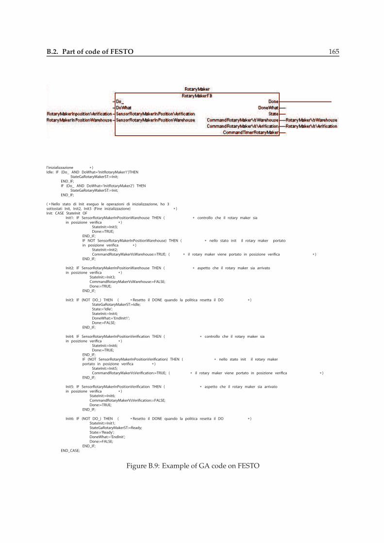
B.2. Part of code of FESTO 165
l’inizializzazione * )Idle: IF (Do_ AND DoWhat=’InitRotaryMaker1’)THEN
StateGaRotaryMakerST:=Init;END_IF;IF (Do_ AND DoWhat=’InitRotaryMaker2’) THEN
StateGaRotaryMakerST:=Init;END_IF;
( * Nello stato di Init eseguo le operazioni di inizializzazione, ho 3sottostati Init, Init2, Init3 (Fine inizializzazione) * )Init: CASE StateInit OF
Init1: IF SensorRotaryMakerInPositionWarehouse THEN ( * controllo che il rotary maker siain posizione veri�ca * )
StateInit:=Init3;Done:=TRUE;
END_IF;IF NOT SensorRotaryMakerInPositionWarehouse) THEN ( * nello stato init il rotary maker portatoin posizione veri�ca * )
StateInit:=Init2;CommandRotaryMakerVsWarehouse:=TRUE; ( * il rotary maker viene portato in posizione veri�ca * )
END_IF;
Init2: IF SensorRotaryMakerInPositionWarehouse THEN ( * aspetto che il rotary maker sia arrivatoin posizione veri�ca * )
StateInit:=Init3;CommandRotaryMakerVsWarehouse:=FALSE;Done:=TRUE;
END_IF;
Init3: IF (NOT DO_) THEN ( * Resetto il DONE quando la politica resetta il DO * )StateGaRotaryMakerST:=Idle;State:=’Idle’;StateInit:=Init4;DoneWhat:=’EndInit1’;Done:=FALSE;
END_IF;
Init4: IF SensorRotaryMakerInPositionVeri�cation THEN ( * controllo che il rotary maker siain posizione veri�ca * )
StateInit:=Init6;Done:=TRUE;
END_IF;IF (NOT SensorRotaryMakerInPositionVeri�cation) THEN ( * nello stato init il rotary makerportato in posizione veri�ca * )
StateInit:=Init5;CommandRotaryMakerVsVeri�cation:=TRUE; ( * il rotary maker viene portato in posizione veri�ca * )
END_IF;
Init5: IF SensorRotaryMakerInPositionVeri�cation THEN ( * aspetto che il rotary maker sia arrivatoin posizione veri�ca * )
StateInit:=Init6;CommandRotaryMakerVsVeri�cation:=FALSE;Done:=TRUE;
END_IF;
Init6: IF (NOT DO_) THEN ( * Resetto il DONE quando la politica resetta il DO * )StateInit:=Init1;StateGaRotaryMakerST:=Ready;State:=’Ready’;DoneWhat:=’EndInit’;Done:=FALSE;
END_IF;END_CASE;
Figure B.9: Example of GA code on FESTO

166 The demonstrator
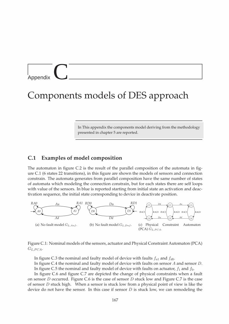
Appendix CComponents models of DES approach
In This appendix the components model deriving from the methodologypresented in chapter 5 are reported.
C.1 Examples of model composition
The automaton in figure C.2 is the result of the parallel composition of the automata in fig-ure C.1 (6 states 22 transitions), in this figure are shown the models of sensors and connectionconstrain. The automata generates from parallel composition have the same number of statesof automata which modeling the connection constrain, but for each states there are self loopswith value of the sensors. In blue is reported starting from initial state an activation and deac-tivation sequence, the initial state corresponding to device in deactivate position.
A0 A1
Ad
AuRA0 RA1
(a) No fault model GL,Anf .
D0 D1
Dd
DuRD0 RD1
(b) No fault model GL,Dnf .
C0
C1Au
AdDu
Dd
RAC0
C5
C2
C4
C3
RAC1 RAC0RAC1 RAC0RAC1
(c) Physical Constraint Automaton(PCA) GL,PCA.
Figure C.1: Nominal models of the sensors, actuator and Physical Constraint Automaton (PCA)GL,PCA.
In figure C.3 the nominal and faulty model of device with faults fa1 and fd0.In figure C.4 the nominal and faulty model of device with faults on sensor A and sensor D.In figure C.5 the nominal and faulty model of device with faults on actuator, f1 and f0.In figure C.6 and figure C.7 are depicted the change of physical constraints when a fault
on sensor D occurred. Figure C.6 is the case of sensor D stuck low and Figure C.7 is the caseof sensor D stuck high. When a sensor is stuck low from a physical point of view is like thedevice do not have the sensor. In this case if sensor D is stuck low, we can remodeling the
167

168 Components models of DES approach
A0,C2,D0
A0,C1,D1
A0,C5,D0
A0,C0,D1
A1,C4,D0
A1,C3,D0
RA0
RD0
RAC1
RAC1
RAC0
RA0
RA1
DdAd
RD0
RA0
RA1
RAC1
RD1
RD1
Du
RA0
RAC0
RD0
RAC0
RD0
Au
1
2
3
4
5
6
Activation and
deactivation sequence
Figure C.2: Composition of nominal sensors and PCA.
A0 A1
Ad
AuRA0 RA1
fa1
RA1
AF1
AG1
RA1
fa1
OutA
(a) Fault model of sensor A,GL,Afa1.
D0 D1
fd0
DF0
Dd
DuRD0 RD1
fd0
RD0
DG0RD0
OutD
(b) fault model of sensor D,GL,Dfd0.
C0
C1Au
AdDu
Dd
RAC0
C5
C2
C4
C3
RAC1 RAC0RAC1 RAC0RAC1
OutD
OutA
(c) Physical Constraint Automaton with faults,GL,PCAF
.
device with only sensor A, and the device becomes the device of figure C.6. The model of thisdevice is composed by an automata of 4 states, because now we can have only two sensorsconfiguration, 00 configuration and 01 configuration, this model can be obtained, as it shownin figure C.6(b), from model of PCA automaton. If sensor D is stuck low the model has not togenerate events Au and Ad, for this reason the model on sensorD when occurs fault fd0 evolvesand remains in state DF0. The PCA automaton do not reach states C0 and C1 but evolves onlyin states C2, C3, C4 and C5.
In figure C.8(a) and figure C.8(b) are reported how the physical constraints of the deviceevolves when a fault on actuator occur. It is easy to see that when a fault on actuator occurs thedevice following the movement of the fault.

C.1. Examples of model composition 169
A0,C1,D1
AG1,C3,D0
AF1,C0,D1
A0,C2,D0
AG1,C4,D0
AF1,C1,D1
A1,C3,D0
AG1,C4,DF0
AF1,C1,DG0AF1,C2,D0
A1,C4,DF0
A1,C4,D0
A0,C1,DG0
AF1,C5,DF0
A0,C5,DF0
A0,C5,D0
AF1,C2,DF0
A0,C2,DF0
AG1,C3,DF0
AF1,C0,DG0A1,C3,DF0
A0,C0,DG0
AF1,C5,D0 A0,C0,D1
fd0
RAC1fa1
RAC1
RA0
Ad
RAC0
RD0
RD1
RAC1
OutA
RA0
Du
fd0
RA1
RAC0
RAC1
RAC0
fd0
RD0 RA0
RA1
RAC0
RD0
fa1
fd0
RA1
RAC1
RA0
RA1
RA1
RAC0
fd0
RD0
RA1
RA1
Du
fd0
RAC0
OutA
RA1
Au
RAC0
RD0
fa1
RD0
RD0
RD0
RAC0
RA0
OutD
RD0
RAC1
RD0
fd0
RD1
Au
Dd
OutD
RAC1
RA1
fd0
RAC0
RA1
fa1
RD0
fa1
RD0
fd0
RA1
RA1
RAC0
RA0
RD1
RAC1
RA0
RA0
fd0
fa1
RA1
fa1
RD1
Dd
RAC1
RD0
RAC1
RAC1
RD0
fd0
RAC0
RD0
Ad
RD0
RAC1
RAC0
RD0
fa1
fa1
fa1
RA1
fa1
RD0
RD0
RA1
fa1
fd0
RA1
RD0
Activation and deactivation sequence
Events OutA, OutD
Fault fa1, activation and deactivation sequence
Fault fd0, activation and deactivation sequence
Fault fd and fa, activation and deactivation
Figure C.3: Composition of nominal and faulty model (faults fa1 and fd0).

170 Components models of DES approach
A0 A1
fa0
AF0
Ad
AuRA0 RA1
fa0
RA0
AG0RA0
OutA
fa1
RA1
AF1
AG1
RA1
fa1
OutA
(a) Fault model of sensor A,GL,Afa.
D0 D1
fd0
DF0
Dd
DuRD0 RD1
fd0
RD0
DG0RD0
OutD
fd1
RD1
DF1
DG1
RD1
fd1
OutD
(b) Fault model of sensor D,GL,Dfd.
C0
C1Au
AdDu
Dd
RAC0
C5
C2
C4
C3
RAC1 RAC0RAC1 RAC0RAC1
OutD
OutA
(c) Physical Constraint Automaton with faults,GL,PCAF
.

C.1.
Exam
ples
ofm
odelcom
position
171
AF1,C2,DF0
AG0,C3,DF1
AG0,C3,DF0
A1,C3,DF1
AF0,C5,DF1
A1,C3,DF0
AF0,C5,DF0
A1,C4,D0
AF0,C0,DG1
AG1,C3,DF1
AF0,C0,DG0
AG1,C3,DF0
AF1,C5,DF1 AF1,C5,DF0
AF1,C0,DG1AF1,C0,DG0
A0,C1,DG1A0,C1,DG0
A0,C2,DF1
AG1,C4,D0
A0,C2,DF0
AG0,C4,D0
A0,C2,D0
AF1,C2,D0
AF0,C2,D0
A0,C5,DF1
A0,C5,DF0
A0,C0,D1
A0,C0,DG1
A0,C0,DG0
A0,C5,D0
AF1,C0,D1AF0,C0,D1
AF1,C5,D0AF0,C5,D0
A1,C3,D0
AG0,C4,DF1AG0,C4,DF0
A1,C4,DF1A1,C4,DF0 AF0,C1,DG1
AG1,C3,D0
AF0,C1,DG0
AG1,C4,DF1
AG0,C3,D0
AG1,C4,DF0
A0,C1,D1
AF0,C2,DF1AF0,C2,DF0
AF1,C1,DG1
AF1,C1,D1
AF1,C1,DG0
AF0,C1,D1
AF1,C2,DF1
RAC1
RAC0
RD0
fa0
RA0 RD1
RAC1
RAC1
RAC1 RAC0
fd0
RA1
OutD
fd0
RD1
RA0
RA1
RD0
RAC1
RD1
fa0
fa1
RAC0
RA1
RD0
fd1
RA0
RAC0
RA1
RD0
RD0
fa1
RD0
RD0
RA0
fd0
fd1
RD1
fa0
RAC1
RA1
RA0
RA0
RD0
RD1
RD1
RD0
fa1
fd0
RAC1RAC0
fa1Ad
RAC0
RD1
RA0
RA1
Au
RAC0
RAC1
fa0
RD0
RD0
RA0
RAC1
RAC0
RAC1
RA1
fa1
RA1
RAC0
RD0
fa0
RD1
RAC0
RAC1
fa1 OutA
Dd
Au
RD1
RA0
fa0
RD1
fd0
fd0
Du
RA1
RAC0
OutD
fd0
OutA
RAC1
OutA
RAC1
fd1
fd0
RAC0
RA0
fa1
RD0
fd1
RA0
RA1 RD0
RAC0
RD0
RD0
RAC0
RA1
RD1
RAC1
RA0
RA0
OutD
RAC0
RD1
RAC1
RAC0
RA0
RA1
RD1
fd1
RA0
fa1
RD1
RA0
fa0
RA1
fa0
Au
RA0
Dd
RD0
RA0
OutA fd0
RD1
fd1
fd1
RAC1
OutD
RA0
RAC0
RA0
RA0
RAC0
fd1
fa1
RA0
RAC1
RAC1
OutA
Du
RA1
RA1
RAC0
RD0
RAC1
fa1
OutD
RAC0
RA0
fa0
fd1
fa1
fa1
fd0
fa0
RA0
RA1
RD1
RA1
RD0
fa0
RAC1
fd0
fa1
fd1
OutDOutA
fd1
fa1
Ad
RAC0
RAC1
fa0
fd0
fd0
fd0
fd1
RD1
fd0
fd0
RD1
RD1
fd0
RA0
RA0
RD0
RD0
RAC0
RAC0
RA0
RA1
RD1
RAC1
RD0
RAC0
RA1
fa1
fa0 RAC1
RA0
fd1
RA1
RAC0
fa0
RA1
RAC0
RAC1
RAC1
RAC1
RD0
RD0
RD1
RD0
RAC1
RA1
fd1
fa0
RD0
RA1
RD1
fa0
fa0
RA0
RD1
fd0
fa0
fa1
RD0
fd1
fd1
RAC0
Ad
RA0
RD1
fa1
Du
Dd
RD0
RA1
RD0
fd1
RD0
fd1
fa1
Activation Deactivation sequenceFault fa1 sequenceFault fa0 sequence
Fault fd1 sequenceFault fd0 sequenceFault fd0 fa0, fd0 fa1, fd1 fa0, fd1 fa1 sequence
fd0 fa0fd1 fa0
fd1 fa1
fd0 fa1
Figure
C.4:C
omp
ositionofnom
inalandfau
ltym
odelw
ithfau
ltson
sensorD
andsensor
A.

172 Components models of DES approach
A0 A1
Ad
AuRA0 RA1
(a) No fault model GL,Anf .
D0 D1
Dd
DuRD0 RD1
(b) No fault model GL,Dnf .
Act0 Act1
RAC0 ACu RAC1
ACuACd
f0 f1
f1f0
RAC0, ACu, ACd
ActF1ActF0
ACd
RAC1, ACu, ACd
(c) Fault model on actuator GL,Act.
C0
C1Au
AdDu
Dd
RAC0
C5
C2
C4
C3
RAC1 RAC0RAC1 RAC0RAC1
(d) Physical Constraint Automaton(PCA) GL,PCA.

C.1.
Exam
ples
ofm
odelcom
position
173
A1,C4,D0,ACF1
A0,C0,D1,ACF1 A1,C4,D0,ACF0
A0,C0,D1,ACF0
A0,C0,D1,AC1
A0,C0,D1,AC0
A1,C4,D0,AC1
A1,C4,D0,AC0
A0,C5,D0,ACF1
A0,C5,D0,ACF0
A0,C2,D0,AC1
A0,C5,D0,AC1
A0,C2,D0,AC0
A0,C5,D0,AC0
A0,C1,D1,ACF1
A0,C1,D1,ACF0
A1,C3,D0,ACF1
A1,C3,D0,ACF0
A0,C1,D1,AC1
A0,C1,D1,AC0
A1,C3,D0,AC1
A1,C3,D0,AC0
A0,C2,D0,ACF1
A0,C2,D0,ACF0
RD1
Ad
RD1
Ad
RD0
RA0
ACd
ACd
f0
ACd
Du
RD0
ACd
f0
RAC0
ACu
RD1
RA0
RAC0
RD0
ACd
RD0
ACu
ACd
f1
ACu
RD0
RA1
RD0
RAC1
RA0
ACd
ACu
Au
ACd
Du
ACd
RD0
RA0
RD0
RA0
RA1
ACd
RD0
f1
Ad f0
f0ACd
RA1
RAC1
RA0
RA0
f0
ACu
RAC1
RA1
DdAu
f0
Ad
RAC0
RA1
RA0
Du
RD0
ACd
ACd
RD0
ACd
RAC0
ACu
f1
ACu
f1
ACu
ACu
ACu
RA1
RAC1
ACu
ACu
Du
f0
ACu
f1
f1
Dd
RAC0 ACu
ACd
ACd
f0
Au
RD1
ACd
f1
RA0
ACd
RA1
ACu
f1
ACu
RAC1
RA0
RD0
RD0
RA0
RA1
ACu
RD1
Dd
f0
f0
RA0
RD0
ACu
f0
ACu
ACd
f1
ACu
f0
ACu
ACu
RD0
ACdf1
RA0
RD0
ACd
RD1
ACu
RA0
f1
ACd
ACu
RD1
Au
RD1
RAC1
RA0
RAC0
ACd
f1
RA0
ACd
Dd
Figure
C.5:C
omp
ositionofnom
inalandfau
ltym
odelw
ithfau
ltson
actuator.

174 Components models of DES approach
DA DA00 01
AuRAC1
DA DA00 01
AdRAC0
DA DA00 01
D A
fd0
RAC1
RAC0
(a) Mechanical configuration fault fd0.
C0
C1Au
AdDu
Dd
RAC0
C5
C2
C4
C3
RAC1 RAC0RAC1 RAC0RAC1
(b) New configuration of (PCA) with fault fd0.
Figure C.6: Models of fault fd0.
DA DA10 11
AuRAC1
DA DA10 11
AdRAC0
DA DA10 11
D
fd1 A
RAC1
RAC0
(a) Mechanical configuration fault fd1.
C0
C1Au
AdDu
Dd
RAC0
C5
C2
C4
C3
RAC1 RAC0RAC1 RAC0RAC1
(b) New configuration of (PCA) with fault fd1.
Figure C.7: Models of fault fd1.
C0
C1Au
AdDu
Dd
RAC0
C5
C2
C4
C3
RAC1 RAC0RAC1 RAC0RAC1
(a) New configuration of (PCA) with fault f0.
C0
C1Au
AdDu
Dd
RAC0
C5
C2
C4
C3
RAC1 RAC0RAC1 RAC0RAC1
(b) New configuration of (PCA) with fault f1.
Figure C.8: Models of actuator faults.

C.2. Control and monitoring of low level devices 175
C.2 Control and monitoring of low level devices
AF0,C0,D1,AC0,T3,S12F1,A0,C0,D1,AC0,T0,S12N
AG0,C3,D0,AC1,T3,S8F1,AF0,C2,D0,AC1,T3,S8F1
AG0,C3,D0,AC1,T3,S7F1,A1,C3,D0,AC1,T0,S7N
AG0,C3,D0,AC1,T3,S6F1,A1,C3,D0,AC1,T0,S6N
AF0,C2,D0,AC1,T3,S2F1,AG0,C3,D0,AC1,T3,S2F1
AG0,C3,D0,AC1,T2,S3F1,AF0,C2,D0,AC1,T2,S3F1
A0,C0,D1,AC0,T0,S0N,AF0,C0,D1,AC0,T3,S0F1
AG0,C4,D0,AC0,T3,S9F1,AF0,C5,D0,AC0,T3,S9F1,AF0,C0,D1,AC0,T3,S9F1,A0,C0,D1,AC0,T0,S9N,AG0,C3,D0,AC0,T3,S9F1,A0,C5,D0,AC0,T0,S9N,A1,C4,D0,AC0,T0,S9N,A1,C3,D0,AC0,T0,S9N
AG0,C3,D0,AC1,T3,S1F1,AF0,C2,D0,AC1,T3,S1F1
AF0,C1,D1,AC1,T2,S3F1,AG0,C3,D0,AC1,T2,S3F1,A0,C1,D1,AC1,T1,S3N,A1,C3,D0,AC1,T1,S3N,AF0,C0,D1,AC1,T2,S3F1,AF0,C2,D0,AC1,T2,S3F1,A0,C0,D1,AC1,T1,S3N,A0,C2,D0,AC1,T1,S3N
AF0,C1,D1,AC1,T3,S2F1,AF0,C2,D0,AC1,T3,S2F1,A0,C1,D1,AC1,T0,S2N,A0,C2,D0,AC1,T0,S2N,AF0,C0,D1,AC1,T3,S2F1,A0,C0,D1,AC1,T0,S2N,A1,C3,D0,AC1,T0,S2N,AG0,C3,D0,AC1,T3,S2F1
A0,C0,D1,AC0,T0,S1N,AF0,C0,D1,AC0,T3,S1F1
AG0,C3,D0,AC0,T3,S11F1,AG0,C4,D0,AC0,T3,S11F1,AF0,C0,D1,AC0,T3,S11F1,A0,C0,D1,AC0,T0,S11N,AF0,C5,D0,AC0,T3,S11F1,A0,C5,D0,AC0,T0,S11N
AG0,C3,D0,AC1,T3,S15F1,AF0,C2,D0,AC1,T3,S15F1
AG0,C3,D0,AC1,T2,S5F1,A1,C3,D0,AC1,T1,S5N
AG0,C3,D0,AC1,T3,S8F1,A1,C3,D0,AC1,T0,S8N
AG0,C3,D0,AC1,T2,S4F1,A1,C3,D0,AC1,T1,S4N,A0,C2,D0,AC1,T1,S4N,AF0,C2,D0,AC1,T2,S4F1
AG0,C3,D0,AC1,T2,S4F1,AF0,C2,D0,AC1,T2,S4F1
AG0,C3,D0,AC1,T4,S14F1,AF0,C2,D0,AC1,T4,S14F1
Ade
Rd
Aa
RA0
RTO
RD1
RA1
SC
TO
RD0
RD0
Ra
RTO
TO
Rd
ACu
SC
ACd
ACd
Ra
RA0
ACu
Figure C.9: State concatenation of diagnoser of figure 5.26.

176 Components models of DES approach
AF0,C5,D0,AC0,T3,S9F1,AF0,C0,D1,AC0,T3,S9F1,AF0,C2,D0,AC0,T3,S9F1
AF0,C2,D0,AC1,T3,S8F1
AF0,C0,D1,AC0,T3,S12F1
AF0,C2,D0,AC1,T2,S3F1
AG0,C3,D0,AC1,T3,S15F1
AF0,C0,D1,AC0,T3,S1F1
AG0,C3,D0,AC0,T3,S11F1,AG0,C4,D0,AC0,T3,S11F1,AF0,C0,D1,AC0,T3,S11F1,AF0,C5,D0,AC0,T3,S11F1
AG0,C3,D0,AC1,T4,S14F1
AG0,C4,D0,AC0,T3,S9F1,AF0,C5,D0,AC0,T3,S9F1,AF0,C0,D1,AC0,T3,S9F1,AF0,C2,D0,AC0,T3,S9F1,AG0,C3,D0,AC0,T3,S9F1
AF0,C0,D1,AC0,T3,S0F1
AF0,C1,D1,AC1,T3,S2F1,AF0,C2,D0,AC1,T3,S2F1,AF0,C0,D1,AC1,T3,S2F1
AG0,C3,D0,AC1,T3,S2F1
AF0,C0,D1,AC0,T3,S11F1,AF0,C2,D0,AC0,T3,S11F1,AF0,C5,D0,AC0,T3,S11F1
AG0,C3,D0,AC1,T3,S1F1
AF0,C2,D0,AC1,T3,S2F1
AG0,C4,D0,AC0,T3,S9F1,AF0,C5,D0,AC0,T3,S9F1,AF0,C0,D1,AC0,T3,S9F1,AG0,C3,D0,AC0,T3,S9F1
AF0,C2,D0,AC1,T3,S15F1
AF0,C1,D1,AC1,T2,S3F1,AF0,C0,D1,AC1,T2,S3F1,AF0,C2,D0,AC1,T2,S3F1
AG0,C3,D0,AC1,T2,S4F1
AF0,C2,D0,AC1,T3,S1F1
AG0,C3,D0,AC0,T3,S11F1,AG0,C4,D0,AC0,T3,S11F1,AF0,C0,D1,AC0,T3,S11F1,AF0,C2,D0,AC0,T3,S11F1,AF0,C5,D0,AC0,T3,S11F1
AG0,C3,D0,AC1,T3,S8F1
AF0,C2,D0,AC1,T4,S14F1
AG0,C3,D0,AC1,T2,S3F1
AF0,C2,D0,AC1,T2,S4F1
Ra
RD0
RD1
RA0
SC
ACu
RD1
ACd
RD0
RA0
RA0
Rd
ACu
ACu
ACd
RTO
RD1
RA0
Ade
TO
Ra
Ra
RTO
TO
ACd
RD0
SC
SC
Rd
Figure C.10: State concatenation of diagnoser of figure 5.26.

C.2. Control and monitoring of low level devices 177
Total Diagnoser States = 44
Id = 1
A0,C0,D1,AC0,T0,S0 N
AF0,C0,D1,AC0,T3,S0 F1
Total pairs = 2
Uncertain: F1
Ra -> 2
Id = 2
A0,C0,D1,AC0,T0,S1 N
AF0,C0,D1,AC0,T3,S1 F1
Total pairs = 2
Uncertain: F1
ACu -> 3
Id = 3
AF0,C1,D1,AC1,T3,S2 F1
AF0,C2,D0,AC1,T3,S2 F1
A0,C1,D1,AC1,T0,S2 N
A0,C2,D0,AC1,T0,S2 N
AF0,C0,D1,AC1,T3,S2 F1
A0,C0,D1,AC1,T0,S2 N
A1,C3,D0,AC1,T0,S2 N
AG0,C3,D0,AC1,T3,S2 F1
Total pairs = 8
Uncertain: F1
SC -> 4
Id = 4
AF0,C1,D1,AC1,T2,S3 F1
AG0,C3,D0,AC1,T2,S3 F1
A0,C1,D1,AC1,T1,S3 N
A1,C3,D0,AC1,T1,S3 N
AF0,C0,D1,AC1,T2,S3 F1
AF0,C2,D0,AC1,T2,S3 F1
A0,C0,D1,AC1,T1,S3 N
A0,C2,D0,AC1,T1,S3 N
Total pairs = 8
Uncertain: F1
RD0 -> 5
Id = 5
AG0,C3,D0,AC1,T2,S4 F1
A1,C3,D0,AC1,T1,S4 N
A0,C2,D0,AC1,T1,S4 N
AF0,C2,D0,AC1,T2,S4 F1
Total pairs = 4
Uncertain: F1
TO -> 6
RA1 -> 7
Id = 6
AG0,C3,D0,AC1,T4,S14 F1
AF0,C2,D0,AC1,T4,S14 F1
Total pairs = 2
Certain: F1
RTO -> 8
Id = 7
AG0,C3,D0,AC1,T2,S5 F1
A1,C3,D0,AC1,T1,S5 N
Total pairs = 2
Uncertain: F1
RTO -> 9
Id = 8
AG0,C3,D0,AC1,T3,S15 F1
AF0,C2,D0,AC1,T3,S15 F1
Total pairs = 2
Certain: F1
Ra -> 10
Rd -> 11
Id = 9
AG0,C3,D0,AC1,T3,S6 F1
A1,C3,D0,AC1,T0,S6 N
Total pairs = 2
Uncertain: F1
Aa -> 12
Id = 10
AG0,C3,D0,AC1,T3,S1 F1
AF0,C2,D0,AC1,T3,S1 F1
Total pairs = 2
Certain: F1
ACu -> 13
Id = 11
AG0,C3,D0,AC1,T3,S8 F1
AF0,C2,D0,AC1,T3,S8 F1
Total pairs = 2
Certain: F1
ACd -> 14
Id = 12
AG0,C3,D0,AC1,T3,S7 F1
A1,C3,D0,AC1,T0,S7 N
Total pairs = 2
Uncertain: F1
RA0 -> 15
Rd -> 16
Id = 13
AF0,C2,D0,AC1,T3,S2 F1
AG0,C3,D0,AC1,T3,S2 F1
Total pairs = 2
Certain: F1
SC -> 17
Id = 14
AG0,C4,D0,AC0,T3,S9 F1
AF0,C5,D0,AC0,T3,S9 F1
AF0,C0,D1,AC0,T3,S9 F1
AF0,C2,D0,AC0,T3,S9 F1
AG0,C3,D0,AC0,T3,S9 F1
Total pairs = 5
Certain: F1
RA0 -> 18
Id = 15
AG0,C3,D0,AC1,T3,S15 F1
Total pairs = 1
Certain: F1
Ra -> 19
Rd -> 20
Id = 16
AG0,C3,D0,AC1,T3,S8 F1
A1,C3,D0,AC1,T0,S8 N
Total pairs = 2
Uncertain: F1
ACd -> 21
Id = 17
AG0,C3,D0,AC1,T2,S3 F1
AF0,C2,D0,AC1,T2,S3 F1
Total pairs = 2
Certain: F1
RD0 -> 22
Id = 18
AG0,C3,D0,AC0,T3,S11 F1
AG0,C4,D0,AC0,T3,S11 F1
AF0,C0,D1,AC0,T3,S11 F1
AF0,C2,D0,AC0,T3,S11 F1
AF0,C5,D0,AC0,T3,S11 F1
Total pairs = 5
Certain: F1
RD1 -> 23
Id = 19
AG0,C3,D0,AC1,T3,S1 F1
Total pairs = 1
Certain: F1
ACu -> 24
Id = 20
AG0,C3,D0,AC1,T3,S8 F1
Total pairs = 1
Certain: F1
ACd -> 25
Id = 21
AG0,C4,D0,AC0,T3,S9 F1
AF0,C5,D0,AC0,T3,S9 F1
AF0,C0,D1,AC0,T3,S9 F1
A0,C0,D1,AC0,T0,S9 N
AG0,C3,D0,AC0,T3,S9 F1
A0,C5,D0,AC0,T0,S9 N
A1,C4,D0,AC0,T0,S9 N
A1,C3,D0,AC0,T0,S9 N
Total pairs = 8
Uncertain: F1
RA0 -> 26
Figure C.11: List of state concatenation of diagnoser of figure 5.26.

178 Components models of DES approach
Total Diagnoser States = 44
Id = 22
AG0,C3,D0,AC1,T2,S4 F1
AF0,C2,D0,AC1,T2,S4 F1
Total pairs = 2
Certain: F1
TO -> 6
Id = 23
AF0,C0,D1,AC0,T3,S12 F1
Total pairs = 1
Certain: F1
Ade -> 27
Id = 24
AG0,C3,D0,AC1,T3,S2 F1
Total pairs = 1
Certain: F1
SC -> 28
Id = 25
AG0,C4,D0,AC0,T3,S9 F1
AF0,C5,D0,AC0,T3,S9 F1
AF0,C0,D1,AC0,T3,S9 F1
AG0,C3,D0,AC0,T3,S9 F1
Total pairs = 4
Certain: F1
RA0 -> 29
Id = 26
AG0,C3,D0,AC0,T3,S11 F1
AG0,C4,D0,AC0,T3,S11 F1
AF0,C0,D1,AC0,T3,S11 F1
A0,C0,D1,AC0,T0,S11 N
AF0,C5,D0,AC0,T3,S11 F1
A0,C5,D0,AC0,T0,S11 N
Total pairs = 6
Uncertain: F1
RD1 -> 30
Id = 27
AF0,C0,D1,AC0,T3,S0 F1
Total pairs = 1
Certain: F1
Ra -> 31
Id = 28
AG0,C3,D0,AC1,T2,S3 F1
Total pairs = 1
Certain: F1
RD0 -> 32
Id = 29AG0,C3,D0,AC0,T3,S11 F1
AG0,C4,D0,AC0,T3,S11 F1
AF0,C0,D1,AC0,T3,S11 F1
AF0,C5,D0,AC0,T3,S11 F1
Total pairs = 4
Certain: F1
RD1 -> 23
Id = 30
AF0,C0,D1,AC0,T3,S12 F1
A0,C0,D1,AC0,T0,S12 N
Total pairs = 2
Uncertain: F1
Ade -> 1
Id = 31
AF0,C0,D1,AC0,T3,S1 F1
Total pairs = 1
Certain: F1
ACu -> 33
Id = 32
AG0,C3,D0,AC1,T2,S4 F1
Total pairs = 1
Certain: F1
TO -> 34
Id = 33
AF0,C1,D1,AC1,T3,S2 F1
AF0,C2,D0,AC1,T3,S2 F1
AF0,C0,D1,AC1,T3,S2 F1
Total pairs = 3
Certain: F1
SC -> 35
Id = 34
AG0,C3,D0,AC1,T4,S14 F1
Total pairs = 1
Certain: F1
RTO -> 15
Id = 35
AF0,C1,D1,AC1,T2,S3 F1
AF0,C0,D1,AC1,T2,S3 F1
AF0,C2,D0,AC1,T2,S3 F1
Total pairs = 3
Certain: F1
RD0 -> 36
Id = 36
AF0,C2,D0,AC1,T2,S4 F1
Total pairs = 1
Certain: F1
TO -> 37
Id = 37
AF0,C2,D0,AC1,T4,S14 F1
Total pairs = 1
Certain: F1
RTO -> 38
Id = 38
AF0,C2,D0,AC1,T3,S15 F1
Total pairs = 1
Certain: F1
Ra -> 39
Rd -> 40
Id = 39
AF0,C2,D0,AC1,T3,S1 F1
Total pairs = 1
Certain: F1
ACu -> 41
Id = 40
AF0,C2,D0,AC1,T3,S8 F1
Total pairs = 1
Certain: F1
ACd -> 42
Id = 41
AF0,C2,D0,AC1,T3,S2 F1
Total pairs = 1
Certain: F1
SC -> 43
Id = 42
AF0,C5,D0,AC0,T3,S9 F1
AF0,C0,D1,AC0,T3,S9 F1
AF0,C2,D0,AC0,T3,S9 F1
Total pairs = 3
Certain: F1
RA0 -> 44
Id = 43
AF0,C2,D0,AC1,T2,S3 F1
Total pairs = 1
Certain: F1
RD0 -> 36
Id = 44
AF0,C0,D1,AC0,T3,S11 F1
AF0,C2,D0,AC0,T3,S11 F1
AF0,C5,D0,AC0,T3,S11 F1
Total pairs = 3
Certain: F1
RD1 -> 23
Figure C.12: List of state concatenation of diagnoser of figure 5.26.

C.2. Control and monitoring of low level devices 179
Name Means observable controllableDu Rising signal on sensor D uo ucDd Falling signal on sensor D uo ucRD0 Signal value on sensor D is low o cRD1 Signal value on sensor D is high o cfd0 Fault on sensor D, stuck low uo ucfd1 Fault on sensor D, stuck high uo ucAu Rising signal on sensor A uo ucAd Falling signal on sensor A uo ucRA0 Signal value on sensor A is low o cRA1 Signal value on sensor A is high o cfa0 Fault on sensor A, stuck low uo ucfa1 Fault on sensor A, stuck high uo ucACu Rising signal on actuator o cACd Falling signal on actuator o cRAC0 Movement of actuator to deactivation state uo ucRAC1 Movement of actuator to activation state uo ucf0 Fault on actuator, blocked low uo ucf1 Fault on actuator, blocked high uo ucRa Request of activation o cRde Request of deactivation o cAa Answer of activation o cAde Answer of deactivation o cSC Command to start count of the timer o cRTO Command to reset the timer o cTO Timeout of the timer o c
GL,Anf Nominal model of sensor AGL,Dnf Nominal model of sensor DGL,Actnf Nominal model of actuatorGL,PCA Model of the Physical Constraint Automaton (PCA)GL,Afa0 Model of sensor A with fault fa0
GL,PCA_A Model of the Physical Constraint Automaton (PCA) with fault fa0GL,Tfa0 Model of timer
GL,ConNom Specification of nominal control for the deviceGL,ConDiag Specification of the control with diagnosis for the deviceGL,CompNom Composition of nominal sensors, actuator and PCAGL,Compfa0 Composition of nominal and fa0 faulty model for the deviceGL,DevNom Composition controlled nominal single acting deviceGL,Devfa0 Composition controlled faulty single acting deviceGL,Totfa0 Composition controlled and diagnosis faulty single acting device
Table C.1: List of events and automata models.

180 Components models of DES approach

Bibliography
[1] Sysml. http://www.sysml.org.
[2] 3s Software. 3s-software.
[3] C. Alexander. A pattern language: Towns, Buildings, Construction. Oxford university Press,1997.
[4] B. Vogel-Heuser, D. Friedrich, U. Katzke, D. Witsch. Usability and benefits of uml forplant automation - some research results. atp International No. 1, 3 (2005).
[5] K. Beck and W. Cunningham. OOPSLA-87 Technical Report No. CR-87-43 Using PatternLanguages for Object-Oriented Programs. 1987.
[6] M. Blanke, M. Kinnaert, J. Lunze, and M. Staroswiecki. Diagnosis and fault-tolerant control.Springer-Verlag, 2003.
[7] W. Bolton. Programmable Logic Controllers. Elsevier, 2006.
[8] M. Bonfè and C. Fantuzzi. Mechatronic objects encapsulation in iec 1131-3 norm. IEEEInternational conference on Control Applications, pages 598 – 603, 2000.
[9] M. Bonfè and C. Fantuzzi. Object-oriented approach to plc software design for a man-ufacture machinery using iec 61131-3 norm languages. IEEE International conference onControl Application, 2:850 – 852, 2001.
[10] M. Bonfè and C. Fantuzzi. Design and verification of mechatronic object-oriented modelsfor industrial control systems. IEEE International conference on Emerging Technologies andFactory Automation, 2:253 – 260, 2003.
[11] M. Bonfè and C. Fantuzzi. Application of object-oriented modeling tools to design thelogic control system of a packaging machine. IEEE International conference on Controlapplication Industrial Informatics, pages 506 – 574, 2004.
[12] M. Bonfè and C. Fantuzzi. A practical approach to object-oriented modeling of logiccontrol system for industrial applications. IEEE International conference on Decision andControl, 1:980 – 985, 2004.
[13] M. Bonfè, C. Fantuzzi, and C. Secchi. Behavioural inheritance in object-oriented modelsfor mechatronic systems. International Journal of Manufacturing Research, 1(4):421 – 441,2006.
181

182 Bibliography
[14] C. Bonivento, A. Paoli, and M. Sartini. Parameters optimization in a production line us-ing genetic algorithms. International Conference on Computational Intelligence for Modelling,Control and Automation,, 2008.
[15] D. Brandl. Design patterns for flexible manufacturing. ISA, 2006.
[16] E. Carpanzano, A. Cataldo, and M. Doná. Rapid prototyping test-bed of logic control so-lution for reconfigurable manufacturing systems. IEEE International conference on Emerg-ing Technologies and Factory Automation, 2:621 – 628, 2005.
[17] C.G. Cassandras and S. Lafortune. Introduction to Discrete Event Systems - Second Edition.Springer, 2007.
[18] CASY-DEIS. Auomation engineering laboratory.
[19] G. Cloutier and J. J. Paques. Gemma, the complementary tool of the grafcet. IEEE Inter-national conference on Programmable Control and Automation Technology, pages 1– 10, 1988.
[20] M.O. Cordier and L. Rozé. Diagnosing discrete-event systems : extending the “diagnoserapproach” to deal with telecommunication networks. Journal on Discrete Event DynamicSystems, 12(2):43 – 81, 2002.
[21] M. Courvoisier, M.Combacau, and A. de Bonneval. Control and monitoring of largediscrete event systems: a generic approach. In Proc. of ISIE 93, pages 571–576, 1993.
[22] G. Davis. Introduction to Packaging Machines. Arlington, 1997.
[23] dSPACE GmbH. dspace prototyping systems. http://www.dspaceinc.com.
[24] E. Dumitrescu, A. Girault, H. Marchand, and E. Rutten. Optimal discrete controller syn-thesis for modeling fault-tolerant distributed systems. Proceedings of the 1st IFAC Workshopon Dependable Control of Discrete Systems, 2007.
[25] D. Orive E. Estévez, M. Marcos. Automatic generation of plc automation projects fromcomponent-based models. Int J Adv Manuf Technol, pages 527–540, 2007.
[26] M. Marcos E. Estévez. An approach to use model driven design in industrial automation.13 th IEEE International Conference on Emerging Technologies and Factory Automation, pages62–69, 2008.
[27] E. Faldella, A. Paoli, M. Sartini, and A. Tilli. Hierarchical supervision systems in indus-trial automation: a design procedure based on the generalized actuator concept. Proceed-ings of 17th IFAC WC, pages 69–76, 2008.
[28] E. Faldella, A. Paoli, A. Tilli, M. Sartini, and D. Guidi. Architectural design patternsfor logic control of manufacturing systems: the generalized device. XXII InternationalSymposium on Information, Communication and Automation Technologies, 2009.
[29] L. Ferrarini, R. Brusa, and C. Veber. A pragmatic approach to fault diagnosis in hydrauliccircuits for automated machining: a case study. 4th IEEE Conference on Automation Scienceand Engineering, 2008.
[30] L. Ferrarini, C. Veber, and G. Fogliazza. Iec 61499 implementation of a modular controlmodel for manufacturing system. IEEE International conference on Emerging Technologiesand Factory Automation, 1:7 – 13, 2005.

Bibliography 183
[31] L. Ferrarini, C. Veber, and V. Schirò. A modular modelling and implementation of au-tomation functions for flexible manufacturing systems. ANIPLA international Congress50¡ Anniversary 1956-2006, Methodologies for Emerging Technologies in Auotomation, 2006.
[32] FESTO-Didactic. Assembly station manual, 2003.
[33] FESTO-Didactic. Distribution station manual, 2003.
[34] FESTO-Didactic. Processing station manual, 2003.
[35] FESTO-Didactic. Testing station manual, 2003.
[36] E. Gamma. Design Patterns. Elements of Reusable Object-Oriented Software. Addison-Wesley,1995.
[37] GAMP. Good automated manufacturing practice. www.ispe.org/gamp/.
[38] S. Genc and S. Lafortune. Distributed diagnosis of place-bordered petri nets. IEEE Trans-actions on Automation Science and Engineering, 4(2):206 –T 219, 2007.
[39] A.L. Buczak H. Darabi, M.A. Jafari. A control switching theory for supervisory controlof discrete event systems. IEEE Transactions on Robotics and Automation, 19(1):131 – 137,2003.
[40] N. Ben Hadj-Alouane, S. Lafortune, and F. Lin. Centralized and distributed algorithmsfor on-line synthesis of maximal control policies under partial observation. Discrete EventDynamic Systems: Theory and Applications, 6(4):379 – 427, 1996.
[41] D. Harel. Statecharts: a visual formalism for complex systems. Science of computer pro-gramming, pages 231–274, 1987.
[42] D. Harel. Modeling Reactive Systems With Statecharts : The Statemate Approach. McGraw-Hill, 1998.
[43] A. Hellgren, B. Lennartson, and M. Fabian. Modelling and plc-based implementation ofmodular supervisory control discrete event systems. Proceedings of 6th Int. Workshop onDiscrete Event Systems, 2002.
[44] Standard IEC. IEC 60848 Grafcet specification language for sequential function charts. TheInstitution of Electrical Engineering, 2002.
[45] Standard IEC. Programable controllers - Part 3: Programming language. The Institution ofElectrical Engineering, 2003.
[46] Standard IEC. 61499-1 Function blocks - Part 1: Architecture. The Institution of ElectricalEngineering, 2005.
[47] Standard IEC. 61499-2 Function blocks Ð Part 2: Software tools requirements. The Institutionof Electrical Engineering, 2005.
[48] M. V. Iordache and P. J. Antsaklis. Resilience to failure and reconfigurations in the su-pervision based on place invariants. Proceedings of the 2004 American Control Conference,2004.
[49] ISA. Batch Control Part 1: Models and Terminology. ISA, 1995.

184 Bibliography
[50] ISA. Batch Control Part 2: Data Structures and Guidelines for Languages. ISA, 2001.
[51] ISPE. International society of pharmaceutical engineering. http://www.ispe.org.
[52] S. Jiang and R. Kumar. Diagnosis of repeated failures for discrete event systems withlinear-time temporal logic specifications. IEEE Transactions on Automation Science and En-gineering, 3(1):47 – 59, 2006.
[53] C. B. Jones. Systematic software development using VDM. Prentice-Hall International, 1986.
[54] Kleanthis C. Thramboulidis. Using uml in control and automation: A model drivenapproach. INDIN ’04. 2nd IEEE International Conference, pages 587–593, 24-26 June 2004.
[55] H. Koepetz. Real-time systems: design principles for distributed embedded applications. Real-time systems. Kluwer academic publishers, London, 1997.
[56] R. Leduc, B. Brandin, M. Lawford, and W. M. Wonham. Hierarchical interface-basedsupervisory control, part i: Serial case. IEEE Transactions on Automatic Control, 50(9):1322–1335, 2005.
[57] R. Leduc, M. Lawford, B. Brandin, and W. M. Wonham. Hierarchical interface-basedsupervisory control, part ii: Parale case. IEEE Transactions on Automatic Control, 50(9):1336–1348, 2005.
[58] R. Leduc, M. Lawford, and P. Dai. Hierarchical interface-based supervisory control of aflexible manufacturing system. IEEE Transactions on Control Systems Technology, 14(4):654–668, 2006.
[59] R. W. Lewis. Programming Industrial Control Systems Using IEC 1131-3. IEE Control Engi-neering Series, 1998.
[60] R. W. Lewis. Modelling control system using IEC 61499. The Institution of Electrical Engi-neering, 2001.
[61] J. Lunze. State observation and diagnosis of discrete-event systems described by stochas-tic automata. Journal on Discrete Event Dynamic Systems, 11(4):319 – 369, 2001.
[62] J. M. Machado, B. Denis, J. J. Lesage, J.M. Faure, and C. L. Ferreira da Silva. Logic con-trollers dependability verification using a plant model. Proceedings of 3th IFAC Workshopon Discrete-Event System Design, 2006.
[63] MathWork. Real time workshop. http://www.mathworks.com/products/rtw.
[64] H. E. Merrit. Hydraulic control systems. John Wiley & Sons, Inc. New York-London-Sydney,1967.
[65] S. Moreno and E. Peulot. Le GEMMA: modes de marches et d’arrest, Grafcet de coordinationdes taches, Conceptions des Systemes Automatises de Production surs. Editions Casteillal, 2002.
[66] O.M.G. Uml, v. 1.4, omg specification, 2001. Document N. formal/2001-09-67, 2001,www.omg.org/uml.
[67] O.M.G. Uml, v. 2.0, omg request for proposal, 2003. Document N. ad/2003-03-02, 2003,www.omg.org/uml.

Bibliography 185
[68] A. Paoli and S. Lafortune. Safe diagnosability for fault tolerant supervision of discreteevent systems. Automatica, 41(8):1335 – 1347, 2005.
[69] A. Paoli and S. Lafortune. Diagnosability analysis of a class of hierarchical state ma-chines. Discrete Event Dynamic Systems: Theory and Applications, 18(3):385–413, 2008.
[70] A. Paoli, M. Sartini, and S. Lafortune. A fault tolerant architecture for supervisory controlof discrete event systems. Proceedings of 17th IFAC WC, pages 6542–6547, 2008.
[71] A. Paoli, M. Sartini, E. Morganti, and C. Bonivento. Genetic algorithm for the optimiza-tion of packiing line. ACD Workshop on Advanced Control and Diagnosis, 2007.
[72] A. Paoli, M. Sartini, and A. Tilli. Rapid prototyping of logic control in industrial automa-tion exploiting the generalized actuator concept. 13 th IEEE International Conference onEmerging Technologies and Factory Automation, pages 82–89, 2008.
[73] R.J. Patton, P.M. Frank, and R.N. Clark. Issues of fault diagnosis for dynamical systems.Springer-Verlag, 2000.
[74] A. Philippot, M. Sayed-Mouchaweh, and V. Carre-Menetrier. Distributed modeling ap-proach of discrete manufacturing systems by parts of plant. Proceedings of the 10th Euro-pean Control Conference, 2009.
[75] A. Pnueli. The temporal logic of programs. In Proc. 18th IEEE Symposium on Foundationsof Computer Science, pages 46–57, 1977.
[76] J.M. Roussel and A. Giua. Designing dependable logic controllers using the supervisorycontrol theory. Proceedings of the 16th IFAC World Congress, 2005.
[77] J. Rumbaugh, I. Jacobson, and G. Booch. Unified Modeling Language Reference Manual.Addison-Wesley, 2004.
[78] M. Sampath, R. Sangupta, and S. Lafortune. Diagnosability of discrete event systems.IEEE Transactions on Automatic Control, 40(9):1555 – 1575, 1995.
[79] M. Sampath, R. Sengupta, S. Lafortune, K. Sinnamohideen, and D.C. Teneketzis. Failurediagnosis using discrete-event models. IEEE Transactions on Control Systems Technology,4(2):105 – 124, 1996.
[80] M. Sampath, R. Sengupta, S. Lafortune, K. Sinnamohideen, and D.C. Teneketzis. Failurediagnosis using discrete-event models. IEEE Transactions on Control Systems Technology,4(2):105 – 124, 1996.
[81] M. Sayed-Mouchaweh, A. Philippot, V. Carre-Menetrier, and B. Riera. Fault diagnosisof discrete event systems using components fault-free models. Proceedings of the 20thInternational Workshop on Principles of Diagnosis, 2009.
[82] B. Selic. The real-time uml standard: definition and application. IEEE International con-ference on Design. Automation and Test, pages 770 – 772, 2002.
[83] B. Selic, G. Gullekson, and P. Ward. Real-tim object -oriented modeling. John Willey & Sons,1994.

186 Bibliography
[84] J.M. Spivey. Introducing Z: a specification language and its Formal semantics. Statecharts: avisual formalism for complex systems. Cambridge university press, 1988.
[85] J. Sifakis T. A. Henzinger. The discipline of embedded systems design. IEEE Computer,40(10):32 –40, 2007.
[86] K. C. Thramboulidis. Towards an engineering tool for implementing reusable distributedcontrol system. ACM SIGSOFT Software Engineering Notes, 28(5), 2003.
[87] K. C. Thramboulidis. Model integrated mechatronics-towards a new paradigm in thedevelopment of manufacturing systems. IEEE Transaction on Industrial Informatics, 1:54 –61, 2005.
[88] K. C. Thramboulidis and C. S. Tranoris. Developing a case tool for distributed controlapplication. The Int. Journal of Advanced manufacturing, 28(1-2), 2004.
[89] A. Tilli and A. Paoli. Rule-based composable modelling of industrial automation au-tomata under nominal and faulty conditions. Proceedings of the 7th IFAC Symposium onFault Detection, Supervision and Safety of Technical Processes, 2009.
[90] A. Tilli, A. Paoli, M. Sartini, C. Bonivento, and D. Guidi. Hierarchical and cooperativeapproaches to logic control design in industrial automation. 14th IEEE International Con-ference on Emerging Technologies and Factory Automation, pages 82–89, 2009.
[91] T. Tolio. Design of flexible production system. Springer, 2009.
[92] V. Vyatkin. IEC 61499 Function Blocks for Embedded and Distributed Control Systems Design.Instrumentation Society of America, USA, July 2006.
[93] V. Vyatkin and X. Cai. Design and implementation of a prototype control system ac-cording to iec 61499. IEEE International conference on Emerging Technologies and FactoryAutomation, 2(269-276), 2003.
[94] V. Vyatkin and H. M. Hanisch. Formal modeling and verification in the software en-gineering framework of iec 61499: a way to self-verifying systems. IEEE Internationalconference on Emerging Technologies and Factory Automation, 2(113–118), 2001.
[95] Q. Wen, R. Kumar, J. Huang, and H. Liu. Fault-tolerant supervisory control of discreteevent systems: formalisation and existence results. Proceedings of the 1st IFAC Workshopon Dependable Control of Discrete Systems, 2007.
[96] Q. Wen, R. Kumar, J. Huang, and H. Liu. Weakly fault-tolerant supervisory control ofdiscrete event systems. Proceedings of the 2007 American Control Conference, 2007.
[97] Q. Wen, R. Kumar, J. Huang, and H. Liu. A framework for fault-tolerant control of dis-crete event systems. IEEE Transactions on Automatic Control, 53(8):1839 – 1849, 2008.
[98] W. M. Wonham. Notes on control of discrete event systems. ECE 1636F/1637S2002-2003. Systems Control Group, Dept. of ECE, University of Toronto, URL:www.control.utoronto.ca/people/profs/wonham/wonham.html.
[99] T.-S. Yoo and S. Lafortune. Solvability of centralized supervisory control under partialobservation. Discrete Event Dynamic Systems: Theory and Applications, 16(4):527 – 553,2006.

Bibliography 187
[100] Y. Zhang and J. Jiang. Integrated active fault-tolerant control using imm approach. IEEETransactions on Aerospace. and Electronic Systems, 37(4):1221 – 1235, 2001.

Index
61131-3, 4361131-3 Languages, 45
61499, 47
Accessible part, 142active event function, 141Activity Diagrams, 51admissible, 146alphabet, 140Assembly machines, 26Assembly station, 158automated manufactory system, 33Automated Manufacturing Systems, 23Automated mode, 42
Batch Processes, 29Block Definition Diagram, 53blocking, 142, 147
Class Diagrams, 51Coaccessible part, 143CoDeSys, 152Collaboration Diagrams, 51Complement, 143Component Diagrams, 51Computational Tree Logic, 99Computer numerical control machines, 28Concatenation, 140concatenation, 140Continuos Processes, 30control recipes, 37controllability, 148Controllability and observability theorem, 149controllability condition, 148Controllability theorem, 148controllable, 148controllable events, 146
deadlock, 142Deployment Diagrams, 51design pattern, 35deterministic automaton, 141Diagnosable DES, 125diagnosing-controller, 121Discrete event system, 139Discrete Processes, 30Distribution station, 152double acting cylinder, 81Dynamic fault detection, 115
empty string, 140equipment hierarchy, 37equipment phase, 74equivalent, 141event, 139event set, 139Execution Control, 50Execution Control Chart, 50
Fault Detection and Isolation, 121Fault Tolerant Control, 121Fault tolerant control, 121FB networks, 48FESTO FMS, 152formal methods, 98formal specification, 98Formal verification, 97function block, 47function block diagram, 46
GEMMA, 39Generalized Actuator, 58Generalized Actuator approach, 63GRAFCET, 40, 42
high level fault, 96
188
Index 189
industrial manufacturing automation, 16Inspection machines, 27instruction lists, 45inverse projection, 144ISPE, 37
Kleene-closure, 140
ladder diagram, 45language, 140language generated, 141language marked, 141large scale systems, 15legal behavior, 146Linear Temporal Logic, 99livelock, 142low level fault, 96
Manual mode, 42marked states, 141master recipes, 37mode of operation, 39Model checking, 98
natural projection, 144Non stop production, 39nonblocking, 142, 147Nonblocking Controllability theorem, 148nondeterministic automaton, 142NS88, 39
Object-Oriented, 36Object-oriented programming, 50observability, 149observable, 149observable events, 147observer, 144Operation models, 42
Packaging machines, 28Parallel composition, 143partial-observation supervisor, 147Physical Constraint Automaton, 105prefix, 140Prefix-closure, 140procedure’s state, 37Processing Station, 156Product, 143production equipment capability, 37Production Processes, 29
Program organization Units, 44Programmable logic controller, 33projection, 144
rapid prototyping, 69recipes, 37regular, 145regular expression, 146resource, 44
S88, 36Safe controllability of DES, 125Safe Diagnosable DES], 125Security module, 42semi-formal method, 98sensor, 78Sequence Diagrams, 51sequential function chart, 46SFC, 39SFC elements, 44Single acting devices, 81Software Engineering, 42standard realization, 149State Diagrams, 51Static fault detection, 115strings, 140Structured text, 46substring, 140suffix, 140supervisory control logic, 110
Test machines, 27Testing station, 154the pattern language, 35transition function, 141Trim operation, 143
UML, 36uncontrollable events, 146Unified Modeling Language, 51unobservable events, 144, 147Use Case Diagrams, 51
variables, 44Verification and validation, 97

190 Index

Curriculum vitae
Matteo Sartini was born in Rimini (Italy) on 15 December 1978.He got his diploma degree at Istituto Tecnico Industriale StataleLeonardo Da Vinci in Rimini with the mark of 60/60. He tookhis master degree in Computer Science Engineeering at Univer-sity of Bologna in March 2005 with a master thesis titled "Mod-ellistica mediante sistemi ibridi: applicazione al sistema frizionedriveline in ambiente automotive - Hybrid systems modeling:application to clutch driveline in automotive systems". On Jan-uary 2006 he obtained his professional engeneering degree.In July 2005 he won a research grant supported by the University of Bologna and Emilia-Romagna regional Council for the project titled "Diagnosis and control for fault tolerant au-tomation systems" under the supervision of Prof. Claudio Bonivento.On January 2006 he began his PhD (XXII cycle) and his research activity within D.E.I.S. (Di-partimento di elettronica, Informatica e Sistemistica - Department of Electronics, ComputerScience and Systems) under the supervision of Prof. Claudio Bonivento.In January 2010 he won a research grant supported European Artemis Joint Undertakingfunded project CESAR: Cost-Efficient methods and processes for SAfety Relevant embedded systemsunder the supervision of Dr. Andrea Paoli.His main research interests are: Industrial automation software architectures, Discrete EventSystems, and fault tolerant control architectures in order to obtain safety and tolerance to faults.
191


![[Srijan Wednesday Webinars] Documenting Design Patterns for Cross Functional Product Teams](https://img.pdfslide.net/doc/110x75/55bac7b7bb61eb01118b46f6/srijan-wednesday-webinars-documenting-design-patterns-for-cross-functional-product-teams.jpg)