This article was downloaded by: [Tracy Rogers]On: 24 January 2015, At: 01:52Publisher: Taylor & FrancisInforma Ltd Registered in England and Wales Registered Number: 1072954 Registeredoffice: Mortimer House, 37-41 Mortimer Street, London W1T 3JH, UK

Click for updates

Polar GeographyPublication details, including instructions for authors andsubscription information:http://www.tandfonline.com/loi/tpog20

Arctic sea ice: use of observationaldata and model hindcasts to refinefuture projections of ice extentTracy S. Rogersa, John E. Walsha, Matthew Leonawiczb & MichaelLindgrenb

a International Arctic Research Center, University of Alaska,Fairbanks, AK, USAb Scenarios Network for Alaska and Arctic Planning, University ofAlaska, Fairbanks, AK, USAPublished online: 13 Jan 2015.

To cite this article: Tracy S. Rogers, John E. Walsh, Matthew Leonawicz & Michael Lindgren (2015):Arctic sea ice: use of observational data and model hindcasts to refine future projections of iceextent, Polar Geography, DOI: 10.1080/1088937X.2014.987849

To link to this article: http://dx.doi.org/10.1080/1088937X.2014.987849

PLEASE SCROLL DOWN FOR ARTICLE

Taylor & Francis makes every effort to ensure the accuracy of all the information (the“Content”) contained in the publications on our platform. However, Taylor & Francis,our agents, and our licensors make no representations or warranties whatsoever as tothe accuracy, completeness, or suitability for any purpose of the Content. Any opinionsand views expressed in this publication are the opinions and views of the authors,and are not the views of or endorsed by Taylor & Francis. The accuracy of the Contentshould not be relied upon and should be independently verified with primary sourcesof information. Taylor and Francis shall not be liable for any losses, actions, claims,proceedings, demands, costs, expenses, damages, and other liabilities whatsoever orhowsoever caused arising directly or indirectly in connection with, in relation to or arisingout of the use of the Content.

This article may be used for research, teaching, and private study purposes. Anysubstantial or systematic reproduction, redistribution, reselling, loan, sub-licensing,systematic supply, or distribution in any form to anyone is expressly forbidden. Terms &

Conditions of access and use can be found at http://www.tandfonline.com/page/terms-and-conditions

Dow

nloa

ded

by [

Tra

cy R

oger

s] a

t 01:

52 2

4 Ja

nuar

y 20

15

Arctic sea ice: use of observational data and model hindcasts to refinefuture projections of ice extent

TRACY S. ROGERSa*, JOHN E. WALSHa, MATTHEW LEONAWICZb andMICHAEL LINDGRENb

aInternational Arctic Research Center, University of Alaska, Fairbanks, AK, USA;bScenarios Network for Alaska and Arctic Planning, University of Alaska,

Fairbanks, AK, USA

(Received 18 December 2013; accepted 11 November 2014)

This manuscript presents an evaluation of global climate models to guide futureprojections of Arctic sea ice extent (SIE). Thirty-five model simulations fromCoupled Model Intercomparison Project, Phase 5 were examined to select modelsubsets using comparison to observational data (1979–2013). The study extends

previous work by highlighting the seasonality of sea ice trends, utilizing a multi-step selection process to demonstrate how the timing of an ice-free Arctic varieswith the hindcast performance of the models, and extending the analysis to

include sudden ice loss events (SILE). Although the models’ trends for thehistorical period are generally smaller than observed, the models’ projectedtrends show a similar seasonality, largest in September and smallest in March to

April. A multi-step evaluation process is applied to obtain progressively smallersubsets of the best-performing models. As the number of models retainedbecomes smaller, the simulated historical trend becomes larger and the median

date of a projected ice-free Arctic becomes earlier. An examination of SILEthrough the historical period and model projections from 2014 through 2099shows that SILE can account for between half and all of the future net loss ofSIE. We created an application for exploring sea ice data: http://spark.rstudio.

com/uafsnap/sea_ice_coverage/.

1. Introduction

There is growing literature on the recent decline of pan-Arctic sea ice coverage (e.g.

(Meier et al. 2007, Parkinson and Cavalieri 2008, Overland and Wang 2013, Stroeve

et al. 2012a). Several assessment studies have examined potential consequences of an

ice-diminished or seasonally ice-free Arctic (ACIA 2005, AMSA 2009, SWIPA 2011),

pointing to the need for information about the timing of changes in marine access to

key areas of the Arctic.

Global climate models are the most powerful tools for assessing the future

trajectory of Arctic sea ice cover, including the timing and seasonality of the

disappearance of summer sea ice. However, climate models contain uncertainties and

must be used cautiously in predictive applications; hindcasts (also known as historical

simulations) by global climate models generally underestimate the rate of ice loss

*Corresponding author. Email: tsrogers@alaska.edu

Polar Geography, 2015

http://dx.doi.org/10.1080/1088937X.2014.987849

# 2015 Taylor & Francis

Dow

nloa

ded

by [

Tra

cy R

oger

s] a

t 01:

52 2

4 Ja

nuar

y 20

15

relative to the observed rate of the past few decades (Stroeve et al. 2012a). Otherevaluations of global climate model simulations of Arctic sea ice extent (SIE),including both hindcasts for recent decades and projections for the remainder of thetwenty-first century have been reported by Arzel et al. (2006), Zhang and Walsh(2006), Massonnet et al. (2012), Rogers et al. (2013), Liu et al. (2013), Overland andWang (2013), among others.

The latest generation of models, from the Coupled Model IntercomparisonProject, Phase 5 (CMIP5), has been found to show marginal improvement over theprevious generation in the ability to capture the overall loss of Arctic sea iceduring the past few decades (Overland and Wang 2013, Stroeve et al. 2012b). Inthis study, we extend previous work with (1) the addition of two contrasting yearsof summer sea ice changes (2012 and 2013), (2) highlighting the significance of theseasonality of sea ice trends, (3) utilizing a two-step model selection process toidentify best-performing models, and (4) extending the analysis to include suddenice loss events (SILE). The objective of this study is two-fold: (1) an evaluation ofclimate models using observed data and hindcasts and (2) investigating the timingand seasonality of the loss of Arctic sea ice over the remainder of the twenty-firstcentury.

2. Observed SIE, 1979–2013

Observed SIE data from 1979 to 2011 were obtained from the National Snow andIce Data Center’s passive microwave bootstrap data-set (Comiso 1995, 1999,Comiso and Kwok 1996). 2012 and 2013 are from NSIDC’s sea ice index (Fettereret al. 2002, Meier et al. 2008), which uses a different algorithm for calculating seaice. The sea ice data were interpolated from their original resolution (∼12.5 km) to a0.4° by 0.4° resolution grid by averaging nearby cells for the purpose of comparisonto global climate model output in the next part of this study. While a coarserresolution has decreased accuracy, this loss is rarely significant and a compromisewas necessary for comparison with global model output in Section 3. Each pixelwith sea ice presence (15% or more sea ice) was converted into an area using thecosine of the latitude multiplied by 12,347 km2 (area inside a 1° latitude by 1°longitude pixel at the Equator). We performed linear regression analyses to estimatesea ice trends.

Our evaluation of sea ice trends identified significant negative pan-Arctictrends in summer months (Table 1). Especially with the inclusion of 2012 and2013, Arctic sea ice has continued to decline rapidly in summer months andmore slowly in winter months. We tested each trend against the null hypothesisthat its trend was zero. We used confidence intervals at 95% to determinethe necessary sample size to reach significance, and then calculated the effectivesample size (which accounts for the effect of autocorrelation on years andsignificance) to determine whether that trend was significant, using thefollowing equation:

eff ¼ n � 1� ar

1þ ar

where eff is the effective sample size, n is the actual sample size, and ar is theautoregression (of the not detrended time series) at a lag of 1 year. When analyzed

2 T. S. Rogers et al.

Dow

nloa

ded

by [

Tra

cy R

oger

s] a

t 01:

52 2

4 Ja

nuar

y 20

15

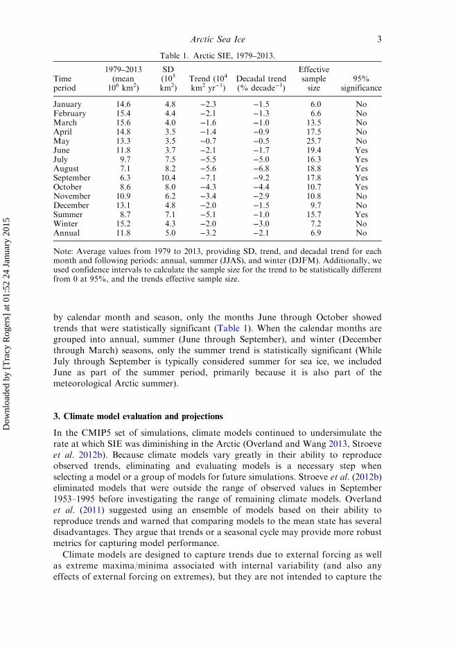
by calendar month and season, only the months June through October showedtrends that were statistically significant (Table 1). When the calendar months aregrouped into annual, summer (June through September), and winter (Decemberthrough March) seasons, only the summer trend is statistically significant (WhileJuly through September is typically considered summer for sea ice, we includedJune as part of the summer period, primarily because it is also part of themeteorological Arctic summer).

3. Climate model evaluation and projections

In the CMIP5 set of simulations, climate models continued to undersimulate therate at which SIE was diminishing in the Arctic (Overland and Wang 2013, Stroeveet al. 2012b). Because climate models vary greatly in their ability to reproduceobserved trends, eliminating and evaluating models is a necessary step whenselecting a model or a group of models for future simulations. Stroeve et al. (2012b)eliminated models that were outside the range of observed values in September1953–1995 before investigating the range of remaining climate models. Overlandet al. (2011) suggested using an ensemble of models based on their ability toreproduce trends and warned that comparing models to the mean state has severaldisadvantages. They argue that trends or a seasonal cycle may provide more robustmetrics for capturing model performance.

Climate models are designed to capture trends due to external forcing as wellas extreme maxima/minima associated with internal variability (and also anyeffects of external forcing on extremes), but they are not intended to capture the

Table 1. Arctic SIE, 1979–2013.

Timeperiod

1979–2013(mean

106 km2)

SD(105

km2)Trend (104

km2 yr−1)Decadal trend(% decade−1)

Effectivesamplesize

95%significance

January 14.6 4.8 −2.3 −1.5 6.0 NoFebruary 15.4 4.4 −2.1 −1.3 6.6 NoMarch 15.6 4.0 −1.6 −1.0 13.5 NoApril 14.8 3.5 −1.4 −0.9 17.5 NoMay 13.3 3.5 −0.7 −0.5 25.7 NoJune 11.8 3.7 −2.1 −1.7 19.4 YesJuly 9.7 7.5 −5.5 −5.0 16.3 YesAugust 7.1 8.2 −5.6 −6.8 18.8 YesSeptember 6.3 10.4 −7.1 −9.2 17.8 YesOctober 8.6 8.0 −4.3 −4.4 10.7 YesNovember 10.9 6.2 −3.4 −2.9 10.8 NoDecember 13.1 4.8 −2.0 −1.5 9.7 NoSummer 8.7 7.1 −5.1 −1.0 15.7 YesWinter 15.2 4.3 −2.0 −3.0 7.2 NoAnnual 11.8 5.0 −3.2 −2.1 6.9 No

Note: Average values from 1979 to 2013, providing SD, trend, and decadal trend for eachmonth and following periods: annual, summer (JJAS), and winter (DJFM). Additionally, weused confidence intervals to calculate the sample size for the trend to be statistically differentfrom 0 at 95%, and the trends effective sample size.

Arctic Sea Ice 3

Dow

nloa

ded

by [

Tra

cy R

oger

s] a

t 01:

52 2

4 Ja

nuar

y 20

15

timing of extreme events, e.g. SILE. This kind of internal variability adds

uncertainty to trends and means for shorter periods. Overland et al. (2011) noted

that comparing trends in periods as long as 20–50 years may be problematic due

to internal variability. Nevertheless, Kay et al. (2011) found that, while a 10-year

trend has the same sign as externally forced trends approximately 66% of the

time, a 20-year time period is sufficient for a model (CCSM3) to capture the sign

of an externally forced trend with 95% confidence. On the basis of their findings,

the 35-year period used in this evaluation is likely to capture an underlying

trend.

To initiate this study, we examine trends in output from 1979 to 2013 in 35

CMIP5 models from 17 climate modeling centers (see the full list of models in

Appendix 1). For the model evaluation process, one goal was to examine the

effect that model selection had on hindcasts and, subsequently, on simulations

through 2099. Some papers have used a ranking system for climate models to

determine an even smaller selection of models for more targeted projection and

scenarios work (Rogers et al. 2013, Walsh et al. 2008). We test whether hindcasts

are improved by two stages of filtering: from 35 to 16 models and from 16 to 5

models. Our first elimination step is to remove models based on deviation from

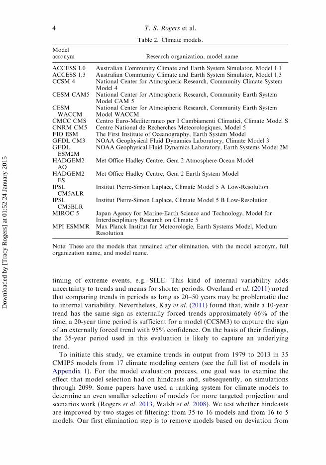
Table 2. Climate models.

Modelacronym Research organization, model name

ACCESS 1.0 Australian Community Climate and Earth System Simulator, Model 1.1ACCESS 1.3 Australian Community Climate and Earth System Simulator, Model 1.3CCSM 4 National Center for Atmospheric Research, Community Climate System

Model 4CESM CAM5 National Center for Atmospheric Research, Community Earth System

Model CAM 5CESMWACCM

National Center for Atmospheric Research, Community Earth SystemModel WACCM

CMCC CMS Centro Euro-Mediterraneo per I Cambiamenti Climatici, Climate Model SCNRM CM5 Centre National de Recherches Meteorologiques, Model 5FIO ESM The First Institute of Oceanography, Earth System ModelGFDL CM3 NOAA Geophysical Fluid Dynamics Laboratory, Climate Model 3GFDLESM2M

NOAA Geophysical Fluid Dynamics Laboratory, Earth Systems Model 2M

HADGEM2AO

Met Office Hadley Centre, Gem 2 Atmosphere-Ocean Model

HADGEM2ES

Met Office Hadley Centre, Gem 2 Earth System Model

IPSLCM5ALR

Institut Pierre-Simon Laplace, Climate Model 5 A Low-Resolution

IPSLCM5BLR

Institut Pierre-Simon Laplace, Climate Model 5 B Low-Resolution

MIROC 5 Japan Agency for Marine-Earth Science and Technology, Model forInterdisciplinary Research on Climate 5

MPI ESMMR Max Planck Institut fur Meteorologie, Earth Systems Model, MediumResolution

Note: These are the models that remained after elimination, with the model acronym, fullorganization name, and model name.

4 T. S. Rogers et al.

Dow

nloa

ded

by [

Tra

cy R

oger

s] a

t 01:

52 2

4 Ja

nuar

y 20

15

the summer and winter means, followed by a ranking based on their summertrend and annual SIE.

3.1. Elimination and evaluation

The simulations used here include hindcasts for the time period 1860–2005, usinghistoric emissions, while model projections for 2006–2099 were based on theRepresentative Concentration Pathways (RCP) 8.5 forcing. We used the first

ensemble member from each available model. Since model resolutions rangedfrom 0.4° by 0.4° to 2.5° by 2.5°, we interpolated all of the models into 0.4° by 0.4°resolution grid, so they shared a common grid with each other and ourinterpolated observed data.

Our first step in the elimination process was to remove models that fell too far

outside the expected range for sea ice, and was based in part on the methods ofStroeve et al. (2012b). We chose the summer time period instead of September

because the range of the observations’ mean September SIE during our evaluationperiod (1979–2013; 3.6–8.1 million km2) was much greater than the range in Stroeve

et al.’s evaluation period (1953–1995; 6.1–8.4 million km2). Based on our Septemberrange, we would have nearly kept every model, despite some modeled values below

5 million km2 before the year 2000. We removed models that were outside theobserved range of summer values (6.7–9.1 million km2) for at least 10 years (out of

35 years). We added an additional metric to eliminate models that did not follow

the seasonal cycle of sea ice – we calculated the difference between the observed

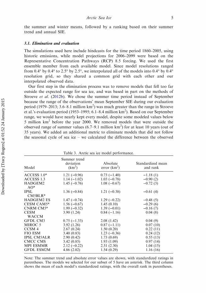
Table 3. Arctic sea ice model performance.

Model

Summer trenddeviation(km2)

Absoluteerror (km2)

Standardized meanand rank

ACCESS 1.0* 1.21 (−0.96) 0.73 (−1.40) −1.18 (1)ACCESS 1.3 1.14 (−1.02) 1.03 (−0.78) −0.90 (2)HADGEM2AO*

1.45 (−0.76) 1.08 (−0.67) −0.72 (3)

IPSLCM5BLR*

1.36 (−0.84) 1.21 (−0.38) −0.61 (4)

HADGEM2 ES 1.47 (−0.74) 1.29 (−0.22) −0.48 (5)CESM CAM5* 1.56 (−0.67) 1.45 (0.10) −0.29 (6)CNRM CM5* 1.99 (−0.32) 1.39 (−0.01) −0.16 (7)CESMWACCM

3.90 (1.24) 0.84 (−1.16) 0.04 (8)

GFDL CM3 0.75 (−1.33) 2.08 (1.42) 0.04 (9)MIROC 5 3.92 (1.26) 0.87 (−1.11) 0.07 (10)CCSM 4 2.67 (0.24) 1.50 (0.20) 0.22 (11)FIO ESM 3.40 (0.83) 1.23 (−0.36) 0.24 (12)IPSL CM5ALR 2.90 (0.42) 1.73 (0.69) 0.55 (13)CMCC CMS 3.42 (0.85) 1.93 (1.09) 0.97 (14)MPI ESMMR 2.12 (−0.22) 2.51 (2.30) 1.04 (15)GFDL ESM2M 4.86 (2.02) 1.54 (0.29) 1.16 (16)

Note: The summer trend and absolute error values are shown, with standardized ratings inparentheses. The models we selected for our subset of 5 have an asterisk. The third columnshows the mean of each model’s standardized ratings, with the overall rank in parentheses.

Arctic Sea Ice 5

Dow

nloa

ded

by [

Tra

cy R

oger

s] a

t 01:

52 2

4 Ja

nuar

y 20

15

mean summer and winter (DJFM) values (7.5 million km2), and eliminated models

that deviated by at least 2.0 million km2 from the observed annual range. This

evaluation criterion is a measure of the model’s sensitivity to forcing by the seasonal

cycle of solar radiation. The first metric eliminated nine models, while the second

metric eliminated 10 models, leaving 16 for comparison (Table 2). Our choice of

evaluation criteria admittedly has some subjectivity. However, these criteria served

the purpose of retaining approximately half the models while eliminating others on

the basis of deficiencies that are transparent to most users who target sea ice

applications of global climate model output.

In order to address the sensitivity to the seasonal definition, we also ran these

elimination steps for the more traditional months of July through September as

summer, and January through March as winter, which resulted in 15 models. Of

these, 13 were among the 16 models from above, indicating that the choice to

include June and December did not have a large effect on model selection.

Our second step was to create a smaller set of models by ranking the remaining

16 models on the basis of (1) their difference from the observed data’s summer

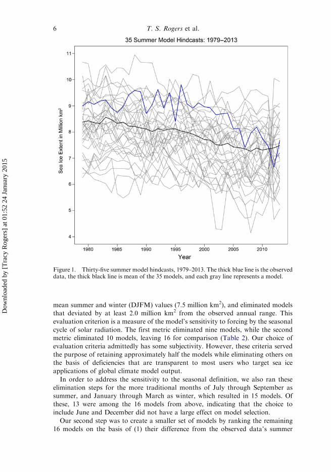
Figure 1. Thirty-five summer model hindcasts, 1979–2013. The thick blue line is the observeddata, the thick black line is mean of the 35 models, and each gray line represents a model.

6 T. S. Rogers et al.

Dow

nloa

ded

by [

Tra

cy R

oger

s] a

t 01:

52 2

4 Ja

nuar

y 20

15

trend and (2) the mean of the absolute value of 12 monthly differences from the

observed data-set:

1

12

X12

i¼1

model mean monthi � observed mean monthij j;

where model mean month represents the model’s mean value for 1979–2013 of the

given calendar month (e.g. January), and the observed mean month is the satellite

observations’ mean for that same month. We then standardized the results from

both metrics to put them on the same scale:

ðxi � �xÞSD

;

where xi is each model’s monthly mean, �xis the mean of all models, and SD is the

standard deviation of xi � �x. We averaged these two standardized values to obtain

our ranking for the models, and used the top five models as a smaller subset of

models. However, to maximize model diversity within such a narrow selection, we

limited models within the top five to one per model center. The resulting top five

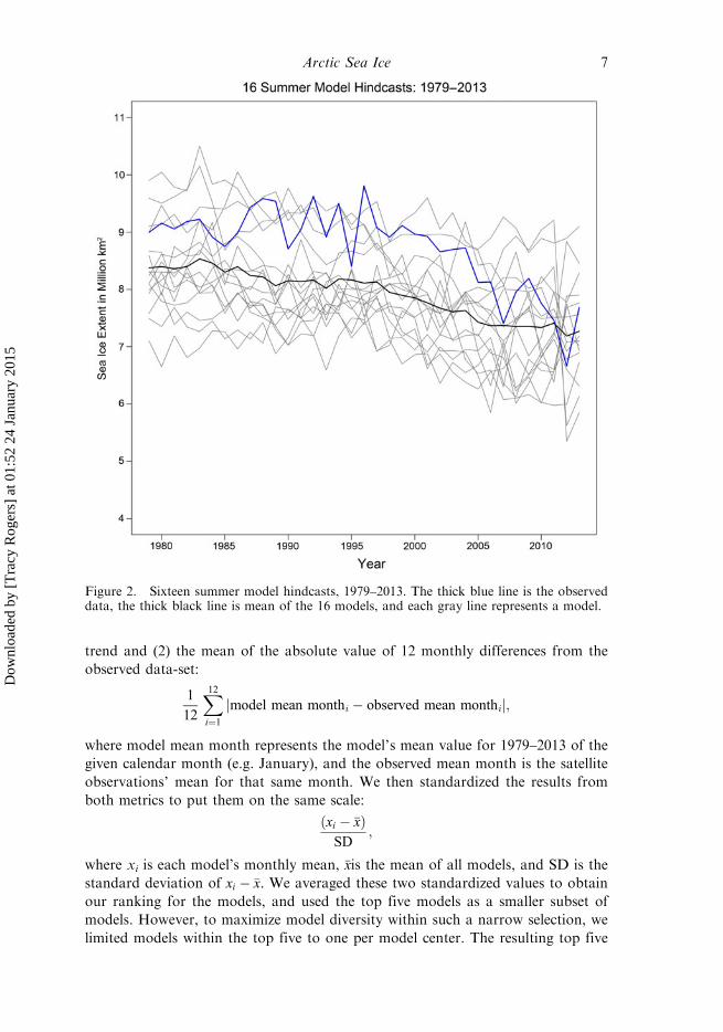
Figure 2. Sixteen summer model hindcasts, 1979–2013. The thick blue line is the observeddata, the thick black line is mean of the 16 models, and each gray line represents a model.

Arctic Sea Ice 7

Dow

nloa

ded

by [

Tra

cy R

oger

s] a

t 01:

52 2

4 Ja

nuar

y 20

15

models were ACCESS 1.0, HADGEM2 AO, IPSL CM5BLR, CESM CAM5, and

CNRM CM5 (Table 3).

When compared with CMIP3 projections in Rogers et al. (2013), more CMIP5

models are effectively capturing the September decline of Arctic sea ice. Stroeve

et al. (2012b) analyzed the difference betwseen CMIP3 and CMIP5 models, and

came to the conclusion that CMIP5 models were more consistent with historical

observations although they noted that some of the improved agreement over the

post-1979 period was the result of a smaller bias in 1979.

September hindcasts from all 35 models are shown in Figure 1, while the hindcasts

from the selected 16 models are shown in Figure 2. It is apparent from Figure 1 that

the models, almost without exception, capture the sign of the underlying trend.

However, the simulated trends are generally smaller than observed, a fact noted by

Stroeve et al. (2012b) and others. A comparison of Figures 1 and 2 shows the observed

trends are reproduced more realistically by the models that survived the initial

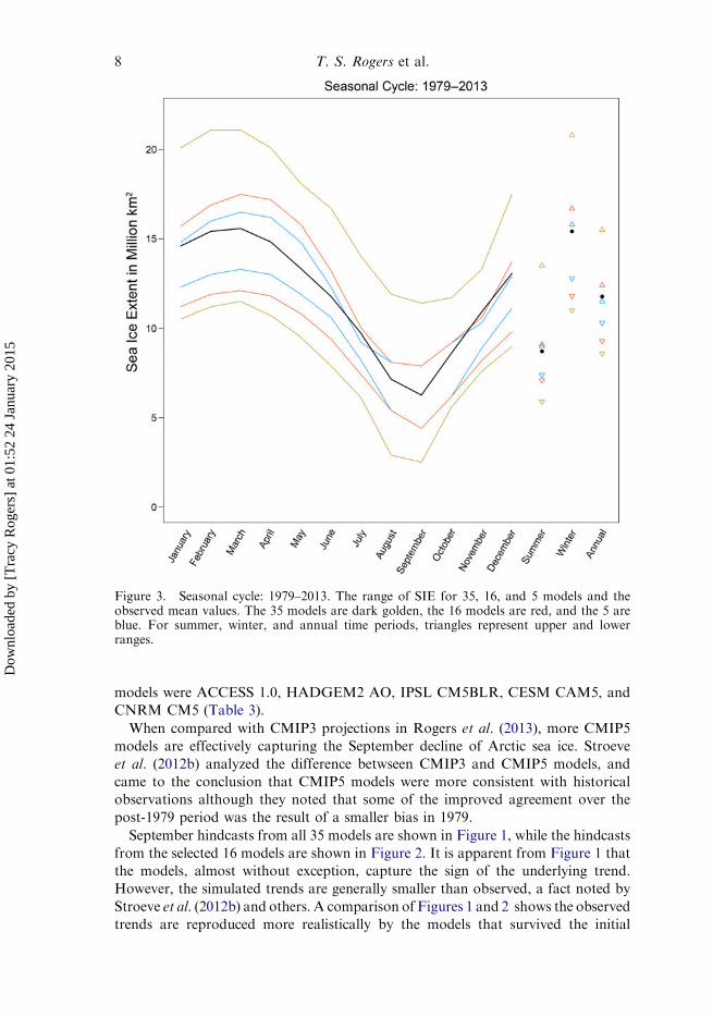
Figure 3. Seasonal cycle: 1979–2013. The range of SIE for 35, 16, and 5 models and theobserved mean values. The 35 models are dark golden, the 16 models are red, and the 5 areblue. For summer, winter, and annual time periods, triangles represent upper and lowerranges.

8 T. S. Rogers et al.

Dow

nloa

ded

by [

Tra

cy R

oger

s] a

t 01:

52 2

4 Ja

nuar

y 20

15

screening process described above. In particular, many of the 35 models significantlyunderestimated the SIE trend during the time period (Table 3).

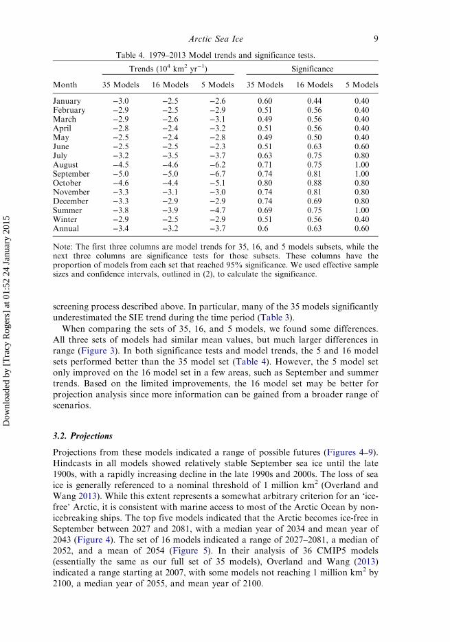
When comparing the sets of 35, 16, and 5 models, we found some differences.All three sets of models had similar mean values, but much larger differences inrange (Figure 3). In both significance tests and model trends, the 5 and 16 modelsets performed better than the 35 model set (Table 4). However, the 5 model setonly improved on the 16 model set in a few areas, such as September and summertrends. Based on the limited improvements, the 16 model set may be better forprojection analysis since more information can be gained from a broader range ofscenarios.

3.2. Projections

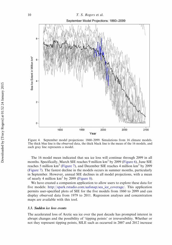
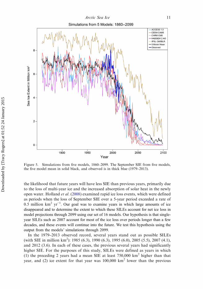
Projections from these models indicated a range of possible futures (Figures 4–9).Hindcasts in all models showed relatively stable September sea ice until the late1900s, with a rapidly increasing decline in the late 1990s and 2000s. The loss of seaice is generally referenced to a nominal threshold of 1 million km2 (Overland andWang 2013). While this extent represents a somewhat arbitrary criterion for an ‘ice-free’ Arctic, it is consistent with marine access to most of the Arctic Ocean by non-icebreaking ships. The top five models indicated that the Arctic becomes ice-free inSeptember between 2027 and 2081, with a median year of 2034 and mean year of2043 (Figure 4). The set of 16 models indicated a range of 2027–2081, a median of2052, and a mean of 2054 (Figure 5). In their analysis of 36 CMIP5 models(essentially the same as our full set of 35 models), Overland and Wang (2013)indicated a range starting at 2007, with some models not reaching 1 million km2 by2100, a median year of 2055, and mean year of 2100.

Table 4. 1979–2013 Model trends and significance tests.

Trends (104 km2 yr−1) Significance

Month 35 Models 16 Models 5 Models 35 Models 16 Models 5 Models

January −3.0 −2.5 −2.6 0.60 0.44 0.40February −2.9 −2.5 −2.9 0.51 0.56 0.40March −2.9 −2.6 −3.1 0.49 0.56 0.40April −2.8 −2.4 −3.2 0.51 0.56 0.40May −2.5 −2.4 −2.8 0.49 0.50 0.40June −2.5 −2.5 −2.3 0.51 0.63 0.60July −3.2 −3.5 −3.7 0.63 0.75 0.80August −4.5 −4.6 −6.2 0.71 0.75 1.00September −5.0 −5.0 −6.7 0.74 0.81 1.00October −4.6 −4.4 −5.1 0.80 0.88 0.80November −3.3 −3.1 −3.0 0.74 0.81 0.80December −3.3 −2.9 −2.9 0.74 0.69 0.80Summer −3.8 −3.9 −4.7 0.69 0.75 1.00Winter −2.9 −2.5 −2.9 0.51 0.56 0.40Annual −3.4 −3.2 −3.7 0.6 0.63 0.60

Note: The first three columns are model trends for 35, 16, and 5 models subsets, while thenext three columns are significance tests for those subsets. These columns have theproportion of models from each set that reached 95% significance. We used effective samplesizes and confidence intervals, outlined in (2), to calculate the significance.

Arctic Sea Ice 9

Dow

nloa

ded

by [

Tra

cy R

oger

s] a

t 01:

52 2

4 Ja

nuar

y 20

15

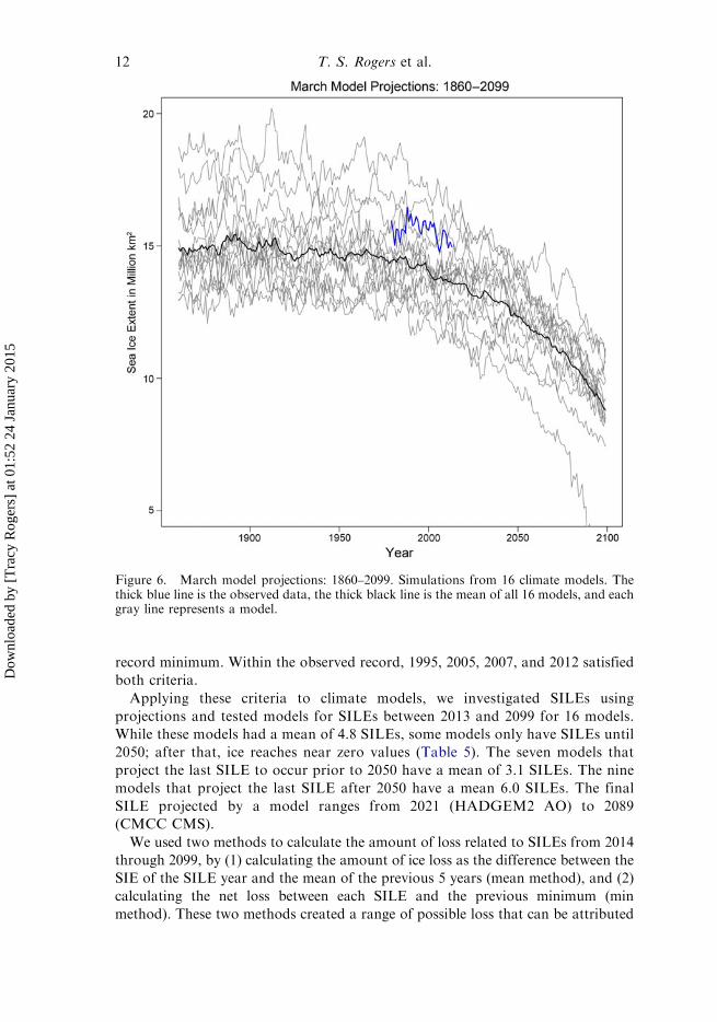
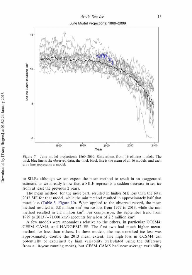
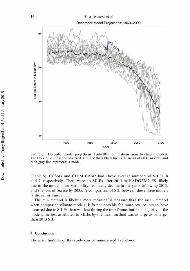
The 16 model mean indicated that sea ice loss will continue through 2099 in allmonths. Specifically, March SIE reaches 9 million km2 by 2099 (Figure 6), June SIEreaches 5 million km2 (Figure 7), and December SIE reaches 4 million km2 by 2099(Figure 7). The fastest decline in the models occurs in summer months, particularlyin September. However, annual SIE declines in all model projections, with a meanof nearly 4 million km2 by 2099 (Figure 8).

We have created a companion application to allow users to explore these data forfive models: http://spark.rstudio.com/uafsnap/sea_ice_coverage/. This applicationpermits user-specified plots of SIE for the five models from 1860 to 2099 and candisplay observed data from 1979 to 2011. Regression analyses and concentrationmaps are available with this tool.

3.3. Sudden ice loss events

The accelerated loss of Arctic sea ice over the past decade has prompted interest inabrupt changes and the possibility of ‘tipping points’ or irreversibility. Whether ornot they represent tipping points, SILE such as occurred in 2007 and 2012 increase

Figure 4. September model projections: 1860–2099. Simulations from 16 climate models.The thick blue line is the observed data, the thick black line is the mean of the 16 models, andeach gray line represents a model.

10 T. S. Rogers et al.

Dow

nloa

ded

by [

Tra

cy R

oger

s] a

t 01:

52 2

4 Ja

nuar

y 20

15

the likelihood that future years will have less SIE than previous years, primarily due

to the loss of multi-year ice and the increased absorption of solar heat in the newly

open water. Holland et al. (2008) examined rapid ice loss events, which were defined

as periods when the loss of September SIE over a 5-year period exceeded a rate of

0.5 million km2 yr−1. Our goal was to examine years in which large amounts of icedisappeared and to determine the extent to which these SILEs account for net ice loss inmodel projections through 2099 using our set of 16 models. Our hypothesis is that single-year SILEs such as 2007 account for most of the ice loss over periods longer than a fewdecades, and these events will continue into the future. We test this hypothesis using theoutput from the models’ simulations through 2099.

In the 1979–2013 observed record, several years stand out as possible SILEs

(with SIE in million km2): 1985 (6.3), 1990 (6.3), 1995 (6.0), 2005 (5.5), 2007 (4.1),

and 2012 (3.6). In each of these cases, the previous several years had significantly

higher SIE. For the purposes of this study, SILEs were defined as years in which

(1) the preceding 2 years had a mean SIE at least 750,000 km2 higher than that

year, and (2) ice extent for that year was 100,000 km2 lower than the previous

Figure 5. Simulations from five models, 1860–2099. The September SIE from five models,the five model mean in solid black, and observed is in thick blue (1979–2013).

Arctic Sea Ice 11

Dow

nloa

ded

by [

Tra

cy R

oger

s] a

t 01:

52 2

4 Ja

nuar

y 20

15

record minimum. Within the observed record, 1995, 2005, 2007, and 2012 satisfied

both criteria.

Applying these criteria to climate models, we investigated SILEs using

projections and tested models for SILEs between 2013 and 2099 for 16 models.

While these models had a mean of 4.8 SILEs, some models only have SILEs until

2050; after that, ice reaches near zero values (Table 5). The seven models that

project the last SILE to occur prior to 2050 have a mean of 3.1 SILEs. The nine

models that project the last SILE after 2050 have a mean 6.0 SILEs. The final

SILE projected by a model ranges from 2021 (HADGEM2 AO) to 2089

(CMCC CMS).

We used two methods to calculate the amount of loss related to SILEs from 2014

through 2099, by (1) calculating the amount of ice loss as the difference between the

SIE of the SILE year and the mean of the previous 5 years (mean method), and (2)

calculating the net loss between each SILE and the previous minimum (min

method). These two methods created a range of possible loss that can be attributed

Figure 6. March model projections: 1860–2099. Simulations from 16 climate models. Thethick blue line is the observed data, the thick black line is the mean of all 16 models, and eachgray line represents a model.

12 T. S. Rogers et al.

Dow

nloa

ded

by [

Tra

cy R

oger

s] a

t 01:

52 2

4 Ja

nuar

y 20

15

to SILEs although we can expect the mean method to result in an exaggerated

estimate, as we already know that a SILE represents a sudden decrease in sea ice

from at least the previous 2 years.

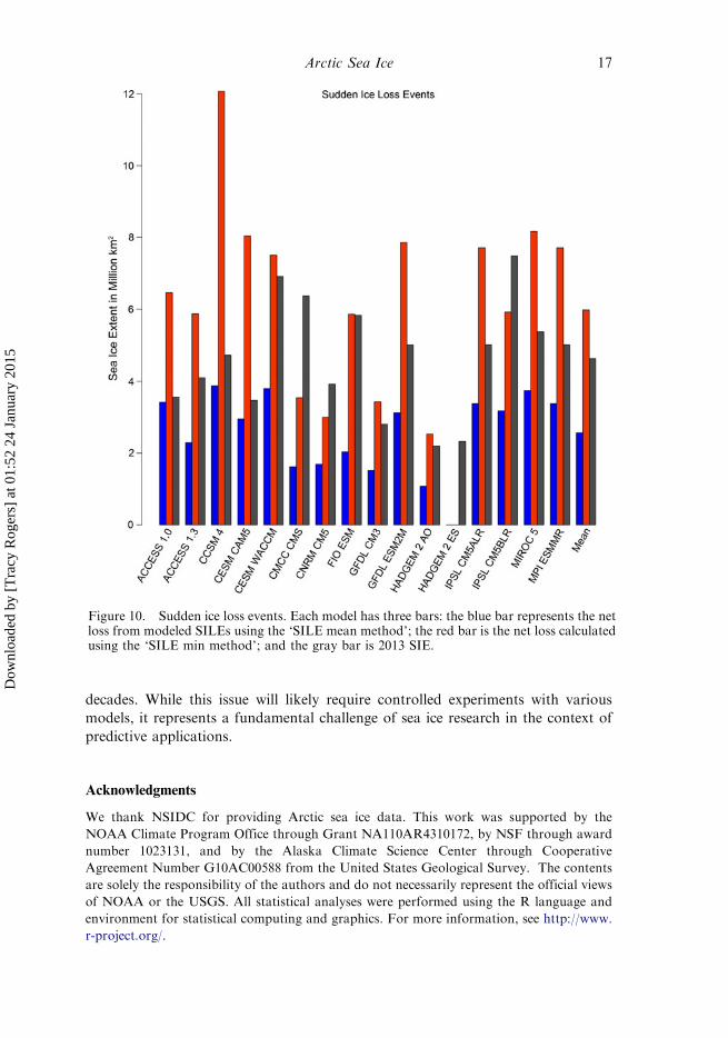
The mean method, for the most part, resulted in higher SIE loss than the total

2013 SIE for that model, while the min method resulted in approximately half that

much loss (Table 5; Figure 10). When applied to the observed record, the mean

method resulted in 3.8 million km2 sea ice loss from 1979 to 2013, while the min

method resulted in 2.2 million km2. For comparison, the September trend from

1979 to 2013 (−71,000 km2) accounts for a loss of 2.5 million km2.

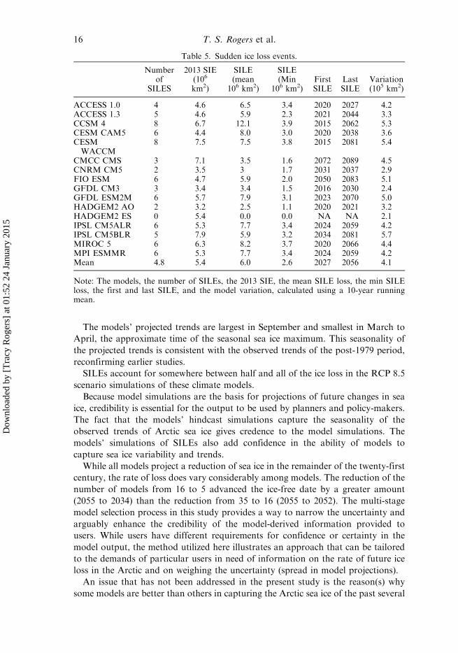
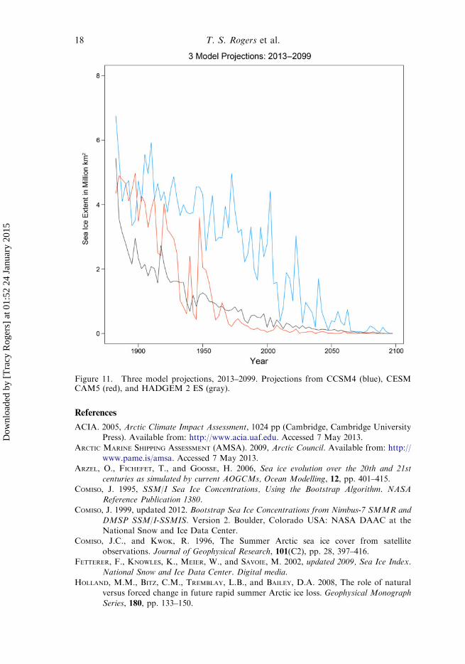
A few models were anomalous relative to the others, in particular CCSM4,

CESM CAM5, and HADGEM2 ES. The first two had much higher mean-

method ice loss than others. In these models, the mean-method ice loss was

approximately double the 2013 mean extent. The high loss in CCSM4 can

potentially be explained by high variability (calculated using the difference

from a 10-year running mean), but CESM CAM5 had near average variability

Figure 7. June model projections: 1860–2099. Simulations from 16 climate models. Thethick blue line is the observed data, the thick black line is the mean of all 16 models, and eachgray line represents a model.

Arctic Sea Ice 13

Dow

nloa

ded

by [

Tra

cy R

oger

s] a

t 01:

52 2

4 Ja

nuar

y 20

15

(Table 5). CCSM4 and CESM CAM5 had above average numbers of SILEs, 8

and 7, respectively. There were no SILEs after 2013 in HADGEM2 ES, likely

due to the model’s low variability, its steady decline in the years following 2013,

and the loss of sea ice by 2035. A comparison of SIE between these three models

is shown in Figure 11.

The min method is likely a more meaningful measure than the mean method

when comparing climate models. It is not possible for more sea ice loss to have

occurred due to SILEs than was lost during the time frame, but, in a majority of the

models, the loss attributed to SILEs by the mean method was as large as or larger

than 2013 SIE.

4. Conclusions

The main findings of this study can be summarized as follows:

Figure 8. December model projections: 1860–2099. Simulations from 16 climate models.The thick blue line is the observed data, the thick black line is the mean of all 16 models, andeach gray line represents a model.

14 T. S. Rogers et al.

Dow

nloa

ded

by [

Tra

cy R

oger

s] a

t 01:

52 2

4 Ja

nuar

y 20

15

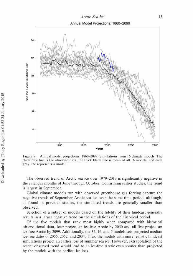
The observed trend of Arctic sea ice over 1979–2013 is significantly negative in

the calendar months of June through October. Confirming earlier studies, the trend

is largest in September.

Global climate models run with observed greenhouse gas forcing capture the

negative trends of September Arctic sea ice over the same time period, although,

as found in previous studies, the simulated trends are generally smaller than

observed.

Selection of a subset of models based on the fidelity of their hindcast generally

results in a larger negative trend on the simulations of the historical period.

Of the five models that rank most highly when compared with historical

observational data, four project an ice-free Arctic by 2050 and all five project an

ice-free Arctic by 2099. Additionally, the 35, 16, and 5 models sets projected median

ice-free dates of 2055, 2052, and 2034. Thus, the models with more realistic hindcast

simulations project an earlier loss of summer sea ice. However, extrapolation of the

recent observed trend would lead to an ice-free Arctic even sooner than projected

by the models with the earliest ice loss.

Figure 9. Annual model projections: 1860–2099. Simulations from 16 climate models. Thethick blue line is the observed data, the thick black line is mean of all 16 models, and eachgray line represents a model.

Arctic Sea Ice 15

Dow

nloa

ded

by [

Tra

cy R

oger

s] a

t 01:

52 2

4 Ja

nuar

y 20

15

The models’ projected trends are largest in September and smallest in March to

April, the approximate time of the seasonal sea ice maximum. This seasonality of

the projected trends is consistent with the observed trends of the post-1979 period,

reconfirming earlier studies.

SILEs account for somewhere between half and all of the ice loss in the RCP 8.5

scenario simulations of these climate models.

Because model simulations are the basis for projections of future changes in sea

ice, credibility is essential for the output to be used by planners and policy-makers.

The fact that the models’ hindcast simulations capture the seasonality of the

observed trends of Arctic sea ice gives credence to the model simulations. The

models’ simulations of SILEs also add confidence in the ability of models to

capture sea ice variability and trends.

While all models project a reduction of sea ice in the remainder of the twenty-first

century, the rate of loss does vary considerably among models. The reduction of the

number of models from 16 to 5 advanced the ice-free date by a greater amount

(2055 to 2034) than the reduction from 35 to 16 (2055 to 2052). The multi-stage

model selection process in this study provides a way to narrow the uncertainty and

arguably enhance the credibility of the model-derived information provided to

users. While users have different requirements for confidence or certainty in the

model output, the method utilized here illustrates an approach that can be tailored

to the demands of particular users in need of information on the rate of future ice

loss in the Arctic and on weighing the uncertainty (spread in model projections).

An issue that has not been addressed in the present study is the reason(s) why

some models are better than others in capturing the Arctic sea ice of the past several

Table 5. Sudden ice loss events.

Numberof

SILES

2013 SIE(106

km2)

SILE(mean

106 km2)

SILE(Min

106 km2)FirstSILE

LastSILE

Variation(105 km2)

ACCESS 1.0 4 4.6 6.5 3.4 2020 2027 4.2ACCESS 1.3 5 4.6 5.9 2.3 2021 2044 3.3CCSM 4 8 6.7 12.1 3.9 2015 2062 5.3CESM CAM5 6 4.4 8.0 3.0 2020 2038 3.6CESMWACCM

8 7.5 7.5 3.8 2015 2081 5.4

CMCC CMS 3 7.1 3.5 1.6 2072 2089 4.5CNRM CM5 2 3.5 3 1.7 2031 2037 2.9FIO ESM 6 4.7 5.9 2.0 2050 2083 5.1GFDL CM3 3 3.4 3.4 1.5 2016 2030 2.4GFDL ESM2M 6 5.7 7.9 3.1 2023 2070 5.0HADGEM2 AO 2 3.2 2.5 1.1 2020 2021 3.2HADGEM2 ES 0 5.4 0.0 0.0 NA NA 2.1IPSL CM5ALR 6 5.3 7.7 3.4 2024 2059 4.2IPSL CM5BLR 5 7.9 5.9 3.2 2034 2081 5.7MIROC 5 6 6.3 8.2 3.7 2020 2066 4.4MPI ESMMR 6 5.3 7.7 3.4 2024 2059 4.2Mean 4.8 5.4 6.0 2.6 2027 2056 4.1

Note: The models, the number of SILEs, the 2013 SIE, the mean SILE loss, the min SILEloss, the first and last SILE, and the model variation, calculated using a 10-year runningmean.

16 T. S. Rogers et al.

Dow

nloa

ded

by [

Tra

cy R

oger

s] a

t 01:

52 2

4 Ja

nuar

y 20

15

decades. While this issue will likely require controlled experiments with various

models, it represents a fundamental challenge of sea ice research in the context of

predictive applications.

Acknowledgments

We thank NSIDC for providing Arctic sea ice data. This work was supported by the

NOAA Climate Program Office through Grant NA110AR4310172, by NSF through award

number 1023131, and by the Alaska Climate Science Center through Cooperative

Agreement Number G10AC00588 from the United States Geological Survey. The contents

are solely the responsibility of the authors and do not necessarily represent the official views

of NOAA or the USGS. All statistical analyses were performed using the R language and

environment for statistical computing and graphics. For more information, see http://www.

r-project.org/.

Figure 10. Sudden ice loss events. Each model has three bars: the blue bar represents the netloss from modeled SILEs using the ‘SILE mean method’; the red bar is the net loss calculatedusing the ‘SILE min method’; and the gray bar is 2013 SIE.

Arctic Sea Ice 17

Dow

nloa

ded

by [

Tra

cy R

oger

s] a

t 01:

52 2

4 Ja

nuar

y 20

15

References

ACIA. 2005, Arctic Climate Impact Assessment, 1024 pp (Cambridge, Cambridge UniversityPress). Available from: http://www.acia.uaf.edu. Accessed 7 May 2013.

ARCTIC MARINE SHIPPING ASSESSMENT (AMSA). 2009, Arctic Council. Available from: http://www.pame.is/amsa. Accessed 7 May 2013.

ARZEL, O., FICHEFET, T., and GOOSSE, H. 2006, Sea ice evolution over the 20th and 21st

centuries as simulated by current AOGCMs, Ocean Modelling, 12, pp. 401–415.COMISO, J. 1995, SSM/I Sea Ice Concentrations, Using the Bootstrap Algorithm. NASA

Reference Publication 1380.

COMISO, J. 1999, updated 2012. Bootstrap Sea Ice Concentrations from Nimbus-7 SMMR andDMSP SSM/I-SSMIS. Version 2. Boulder, Colorado USA: NASA DAAC at theNational Snow and Ice Data Center.

COMISO, J.C., and KWOK, R. 1996, The Summer Arctic sea ice cover from satellite

observations. Journal of Geophysical Research, 101(C2), pp. 28, 397–416.FETTERER, F., KNOWLES, K., MEIER, W., and SAVOIE, M. 2002, updated 2009, Sea Ice Index.

National Snow and Ice Data Center. Digital media.

HOLLAND, M.M., BITZ, C.M., TREMBLAY, L.B., and BAILEY, D.A. 2008, The role of naturalversus forced change in future rapid summer Arctic ice loss. Geophysical MonographSeries, 180, pp. 133–150.

Figure 11. Three model projections, 2013–2099. Projections from CCSM4 (blue), CESMCAM5 (red), and HADGEM 2 ES (gray).

18 T. S. Rogers et al.

Dow

nloa

ded

by [

Tra

cy R

oger

s] a

t 01:

52 2

4 Ja

nuar

y 20

15

KAY, J.E., HOLLAND, M.M., and JAHN, A. 2011, Inter-annual to multi-decadal Arctic sea iceextent trends in a warming world, Geophysical Research Letters, 38, p. L15708.

LIU, J., SONG, M., HORTON, R., and HU, Y. 2013, Reducing spread in climate model

projections of a September ice-free Arctic. 2013. Proceedings of the National Academyof Sciences of the United States of America, 110, p. 31.

MASSONNET, F., FICHEFET, T., GOOSSE, H., BITZ, C.M., PHILIPPON-BERTHIER, G., HOLLAND, M.

M., and BARRIAT, P.-Y. 2012, Constraining projections of summer Arctic sea ice. TheCryosphere, 6, pp. 1383–1394.

MEIER, W., FETTERER, F., KNOWLES, K., MEIER, W., SAVOIE, M., and BRODZIK, M.J. 2006, Sea

Ice Concentrations from Nimbus-7 SMMR and DMSP SSM/I Passive MicrowaveData (2008) (Boulder, CO: National Snow and Ice Data Center, Digital Media).

MEIER, W., STROEVE, J., and FETTERER, F. 2007, Whither Arctic sea ice? A clear signal ofdecline regionally, seasonally, and extending beyond the satellite record. Annals of

Glaciology, 46, pp. 428–434.OVERLAND, J.E., and WANG, M. 2013, When will the Summer Arctic be nearly sea ice free?

Geophysical Research Letters, 40, pp. 2097–2101.OVERLAND, J.E., WANG, M., BOND, N., WALSH, J., KATTSOV, V., and CHAPMAN, W. 2011,

Considerations in the selection of global climate models for regional climateprojections: The Arctic as a case study. Journal of Climate, 24, pp. 1583–1597.

PARKINSON, C., and CAVALIERI, D. 2008, Arctic sea ice variability and trends, 1979–2006.Journal of Geophysical Research, 113, p. C07003.

ROGERS, T.S., WALSH, J.E., RUPP, T.S., BRIGHAM, L.W., and SFRAGA, M. 2013, Future Arcticmarine access: Analysis and evaluation of observations, models, and projections of

sea ice. The Cryosphere, 7, pp. 321–332.Snow, Water, Ice and Permafrost in the Arctic (SWIPA). 2011. Climate Change and the

Cryosphere. Arctic Monitoring and Assessment Programme (AMAP), Oslo, Norway.

Available from: http://amap.no/swipa/. Accessed 7 May 2013.STROEVE, J., SERREZE, M., HOLLAND, M., KAY, J., MALANIK, J., and BARRET, A. 2012a, The

Arctic’s rapidly shrinking sea ice cover: a research synthesis. Climatic Change, 110,

pp. 1005–1027.STROEVE, J., KATTSOV, V., BARRET, A., SERREZE, M., PAVLOVA, T., HOLLAND, M., and MEIER,

W. 2012b, Trends in Arctic sea ice extent from CMIP5, CMIP3 and observations.

Geophysical Research Letters, 39, pp. 2097–2101.WALSH, J., CHAPMAN, W., ROMANOVSKY, V., CHRISTENSEN, J., and STENDEL, M. 2008, Global

Climate Model Performance over Alaska and Greenland. Journal of Climate, 21, pp.6156–6174.

ZHANG, X., and WALSH, J. 2006, Toward a seasonally ice-covered arctic ocean: Scenariosfrom the IPCC AR4 model simulations. Journal of Climate, 19, pp. 1730–1747.

Arctic Sea Ice 19

Dow

nloa

ded

by [

Tra

cy R

oger

s] a

t 01:

52 2

4 Ja

nuar

y 20

15

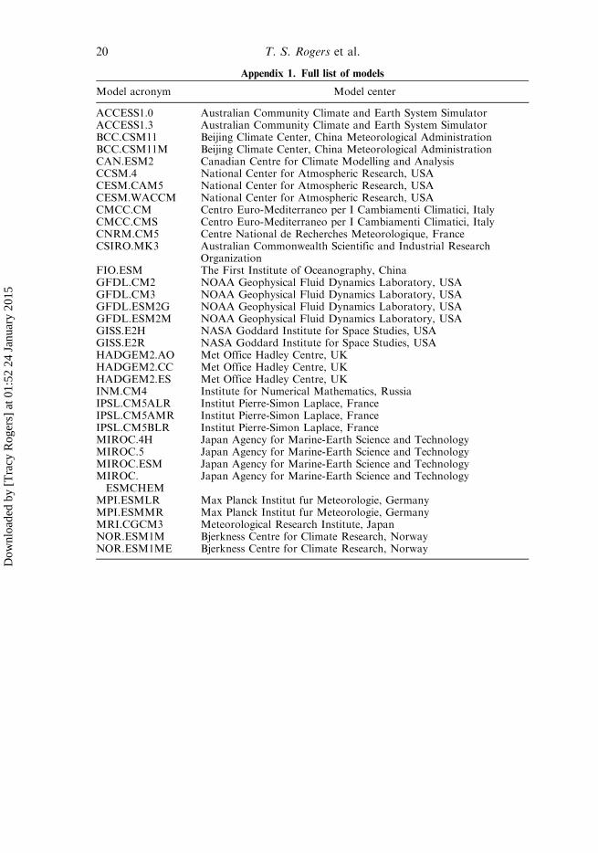
Appendix 1. Full list of models

Model acronym Model center

ACCESS1.0 Australian Community Climate and Earth System SimulatorACCESS1.3 Australian Community Climate and Earth System SimulatorBCC.CSM11 Beijing Climate Center, China Meteorological AdministrationBCC.CSM11M Beijing Climate Center, China Meteorological AdministrationCAN.ESM2 Canadian Centre for Climate Modelling and AnalysisCCSM.4 National Center for Atmospheric Research, USACESM.CAM5 National Center for Atmospheric Research, USACESM.WACCM National Center for Atmospheric Research, USACMCC.CM Centro Euro-Mediterraneo per I Cambiamenti Climatici, ItalyCMCC.CMS Centro Euro-Mediterraneo per I Cambiamenti Climatici, ItalyCNRM.CM5 Centre National de Recherches Meteorologique, FranceCSIRO.MK3 Australian Commonwealth Scientific and Industrial Research

OrganizationFIO.ESM The First Institute of Oceanography, ChinaGFDL.CM2 NOAA Geophysical Fluid Dynamics Laboratory, USAGFDL.CM3 NOAA Geophysical Fluid Dynamics Laboratory, USAGFDL.ESM2G NOAA Geophysical Fluid Dynamics Laboratory, USAGFDL.ESM2M NOAA Geophysical Fluid Dynamics Laboratory, USAGISS.E2H NASA Goddard Institute for Space Studies, USAGISS.E2R NASA Goddard Institute for Space Studies, USAHADGEM2.AO Met Office Hadley Centre, UKHADGEM2.CC Met Office Hadley Centre, UKHADGEM2.ES Met Office Hadley Centre, UKINM.CM4 Institute for Numerical Mathematics, RussiaIPSL.CM5ALR Institut Pierre-Simon Laplace, FranceIPSL.CM5AMR Institut Pierre-Simon Laplace, FranceIPSL.CM5BLR Institut Pierre-Simon Laplace, FranceMIROC.4H Japan Agency for Marine-Earth Science and TechnologyMIROC.5 Japan Agency for Marine-Earth Science and TechnologyMIROC.ESM Japan Agency for Marine-Earth Science and TechnologyMIROC.ESMCHEM

Japan Agency for Marine-Earth Science and Technology

MPI.ESMLR Max Planck Institut fur Meteorologie, GermanyMPI.ESMMR Max Planck Institut fur Meteorologie, GermanyMRI.CGCM3 Meteorological Research Institute, JapanNOR.ESM1M Bjerkness Centre for Climate Research, NorwayNOR.ESM1ME Bjerkness Centre for Climate Research, Norway

20 T. S. Rogers et al.

Dow

nloa

ded

by [

Tra

cy R

oger

s] a

t 01:

52 2

4 Ja

nuar

y 20

15